Spatiotemporal Dynamics of Suspended Sediments in the Negro River, Amazon Basin, from In Situ and Sentinel-2 Remote Sensing Data

Abstract

Monitoring suspended sediments through remote sensing data in black-water rivers is a challenge. Herein, remote sensing reflectance (R_rs) from in situ measurements and Sentinel-2 Multi-Spectral Instrument (MSI) images were used to estimate the suspended sediment concentration (SSC) in the largest black-water river of the Amazon basin. The Negro River exhibits extremely low R_rs values (<0.005 sr⁻¹ at visible and near-infrared bands) due to the elevated absorption of coloured dissolved organic matter (aCDOM at 440 nm > 7 m⁻¹) caused by the high amount of dissolved organic carbon (DOC > 7 mg L⁻¹) and low SSC (<5 mg L⁻¹). Interannual variability of R_rs is primarily controlled by the input of suspended sediments from the Branco River, which is a clear water river that governs the changes in the apparent optical properties of the Negro River, even at distances that are greater than 90 km from its mouth. Better results were obtained using the Sentinel-2 MSI Red band (Band 4 at 665 nm) in order to estimate the SSC, with an R² value greater than 0.85 and an error less than 20% in the adjusted models. The magnitudes of water reflectance in the Sentinel-2 MSI Red band were consistent with in situ R_rs measurements, indicating the large spatial variability of the lower SSC values (0 to 15 mg L⁻¹) in a complex anabranching reach of the Negro River. The in situ and satellite data analysed in this study indicates sedimentation processes in the lower Negro River near the Amazon River. The results suggest that the radiometric characteristics of sensors, like sentinel-2 MSI, are suitable for monitoring the suspended sediment concentration in large tropical black-water rivers.

1. Introduction

As important components of continental landforms, large rivers play a significant role in continental erosion, and they are the main agents for transferring erosion products to the oceans [1,2]. Thus, monitoring sediment transport in large rivers contributes to the understanding of the biogeochemical cycles in order to quantify soil erosion and the formation of landscapes [3,4,5]. However, systematic and regular measurements of sediments by gauging stations in large rivers are not available and they require indirect estimates [1], especially in the tropical region. Therefore, Earth observation satellites have helped to obtain information on suspended sediment in different aquatic systems over the last thirty years, and these instruments have become indispensable for monitoring coastal and inland water bodies [6,7,8].

Satellite images have been used since the late 1970’s to assess the spatial and temporal variability of physical, chemical, and biological properties of water [9,10]. In the coming decades, new missions will be launched to build on existing ones and contribute to decision making [11]. Scientific advances in this technology have helped to create systems that remotely monitor suspended sediment in rivers and lakes. Currently, institutions worldwide use remote water sensing to complement in situ monitoring [12,13,14]. The availability of high frequency data and different orbital platforms facilitate remote water sensing [15]. For instance, combined with other large tropical rivers, studies in the Amazon basin have contributed to recent advances in remotely monitoring sediment concentration [16,17,18,19,20].

The primary characteristics of Amazonian waters are driven by the dynamics of the suspended inorganic sediments originating from the Andes [21]. The high amount of coloured dissolved organic matter is due to the strong degradation of terrestrial organic carbon [22,23] from the surrounding forests. The Negro River has the lowest concentration of suspended sediment and the highest concentration of dissolved organic carbon in the Amazon basin [24,25]. Even for such concentration levels, suspended sediments deeply influence biogeochemical processes, impacting primary productivity and greenhouse gas emissions [26,27]. Therefore, suspended sediment concentration is an important indicator for water quality in natural conditions, as well as a proxy for anthropogenic activities, such as deforestation, mining, or dam facilities on large rivers [28,29,30].

Characteristics, such as elevated light absorption, very low remote sensing reflectance (R_rs) response, and a weak water-leaving signal, make suspended sediment monitoring by passive satellite sensors in large black-water rivers a challenge. However, increased suspended sediment concentration increases the energy that is reflected by the water surface at the visible and near-infrared bands, which enables the use of satellite images to map the spatiotemporal variability of suspended inorganic material in lakes, rivers, and estuaries [18,29,31,32,33,34]. Recent studies indicate that good performance can be obtained between suspended sediment concentration and remote sensing reflectance of inland water bodies [17,35,36,37,38,39] using empirical models with a single band for environments with low (<50 mg L⁻¹) and high concentrations (>100 mg L⁻¹) [34,40,41,42].

In order to estimate the suspended sediment in Amazonian hydrosystems, research focused on rivers originating in the Andes, such as the Solimões and Madeira Rivers [19,43,44], in tributaries, such as the Purus River [45], as well as in the lower Amazon River floodplain [17,46,47]. Few studies have focused on the analysis of suspended sediment and in situ R_rs in Amazonian rivers that are dominated by dissolved organic matter, such as the Negro River. This large river represents 11% of the total Amazon basin area and it contributes 14% of water discharge. It has great ecological importance and it is the main forest ecosystem flooded by black-water (Igapó forest) in the Amazon. This lack of studies with remote sensing data is due to the challenge of working with the low water signal, which reaches an average maximum of 0.5% in the Red band at the water surface level, making radiometric measurements difficult [18,48].

The Negro River basin comprises gauging stations with the lowest densities when compared to those that are situated on the large rivers in the Amazon [49]. On the other hand, advances in remote sensing data and technology can fill the gaps in poorly monitored basins [10,50,51]. With the above approach, the aim of this study was to estimate the suspended sediment concentration in the Negro River using in situ R_rs and Sentinel-2 Multi-Spectral Instrument (MSI) images. Based on radiometric measurements that were collected during different hydrological periods, this study contributes to the understanding of Apparent Optical Properties (AOPs) of water in the rivers that are dominated by dissolved organic matter and very low suspended sediment concentrations.

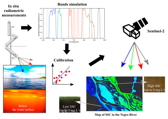
2. Materials and Methods

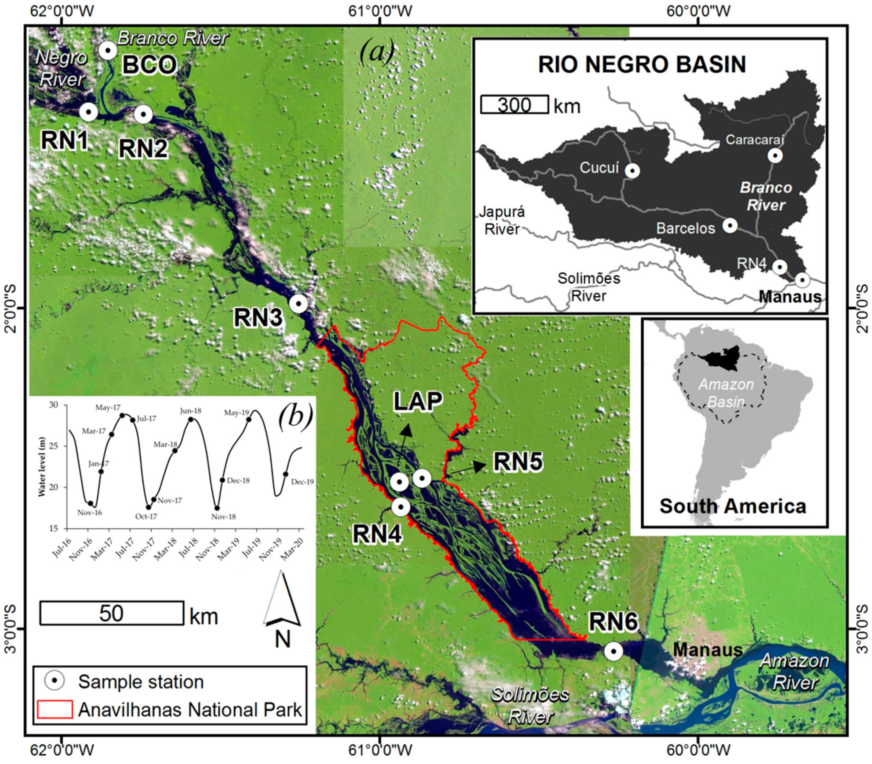
2.1. Study area

The study was conducted along of the lower course of the Negro River, north of the Amazon basin, and between the confluence of the Negro and the Branco rivers and the Anavilhanas National Park (Figure 1a). With 712,000 km² of drainage area and an annual average water flow of 28,000 m³ s⁻¹, the Negro River is a large and complex multichannel river with archipelagos. The Anavilhanas Archipelago is the most notable geomorphological feature in the low course of this river, due to its complex anabranching pattern, with hundreds of islands and floodplain lakes [52].

The total suspended sediment discharge values range from 1 to 7 Mt per year, primarily from the Guyana Shields and savannah areas, with an erosion rate of less than 10 ton. km² year⁻¹ [49,53]. The Branco River, which is the main tributary of the basin in terms of discharge and suspended sediment, has an average annual flow of 3000 m³ s⁻¹ (in Caracaraí station) and it contributes about 50% of the suspended flow in the lower Negro River [53,54]. The mean annual suspended sediment concentration of the Negro and the Branco rivers, based on in-situ data, is ~5 mg L⁻¹ and ~30 mg L⁻¹, respectively [49,55,56,57]. The soils in the basin are covered by dense equatorial forest, poor in nutrients, and formed by the weathering of crystalline rocks [58].

The Rio Negro Basin is located in the geomorphological domains of the Guiana Shields, which consist of highly eroded Precambrian lands with little influence on the dissolved inorganic carbon flows that are carried by the rivers [23]. In this basin, old rocks predominate (granites), and there is not a significant presence of carbonates [59].

The climate in this basin is tropical without a dry season (Af), according to the Köppen classification. The average annual rainfall is 2000 mm, with values exceeding 3500 mm in the Northwest portion of the basin. The annual variability of the water level of the lower Negro River reaches 10 m, with a flood period exceeding seven months. In the study area, the high water and low water periods occur, respectively, between June and July and October and November.

Sioli [60] classified the primary types of water in the Amazonian rivers into three types: rivers with white, black, or clear water. Black-water rivers are typical in the Negro River basin, with the presence of acidic water (pH close to 4), low electrical conductivity (<20 µS), dissolved organic carbon concentration (DOC) over 8 mg L⁻¹, and suspended sediment concentration of less than 10 mg L⁻¹ [25]. With an average chlorophyll-a concentration around 1 µg L⁻¹, the high DOC concentration increases light attenuation in the water column, limiting primary phytoplankton production in the Negro River [61,62].

2.2. In situ Data Collection

Figure 2 presents a flowchart of the methodology that was used in this study. Data acquisition occurred between 2016 and 2019 at eight sample stations that were visited in different water level periods (Figure 1b). Note that the following nomenclature was used to differentiate rivers and lakes: BCO, RN, and LAP stand for Branco River, Negro River, and Lake Apacú, respectively. Three stations are located near the confluence region of the Negro (stations RN1 and RN2) and the Branco Rivers (station BCO). The stations RN1 and RN2 are located upstream and downstream the mouth of the Branco River, respectively. Five stations are situated upstream (RN3), inside (RN4, RN5, and LAP), and downstream (RN6) of the Anavilhanas Archipelago. Inside the Anavilhanas Archipelago, the station LAP is located on Lake Apacú, and stations RN4 and RN5 are situated on channels at the right and left banks of Negro River, respectively. Each sample station corresponds to a fixed coordinate.

2.2.1. Radiometry

Measurements of the remote sensing reflectance, R_rs in sr⁻¹, were performed based on above-water radiometry acquisitions using three TriOS RAMSES spectroradiometers operating in the spectral range 350–950 nm, which is widely used in large Amazonian rivers [18,38,44]. Sensor configuration and data collection geometry were set to follow the protocol that was suggested by Mobley [63], i.e., using a viewing angle of 40° and a relative azimuth from the Sun of 135°. The main principle of above-water radiometry is to correct for the contribution of the surface reflection (mostly skylight) to the measured signal to properly obtain the water-leaving radiance [64]. This step is especially critical for highly absorbing water, where exiting radiances remain low and potentially yield large uncertainty on the retrieved R_rs.

Hundreds of R_rs were calculated with consideration of the impacts of polarisation of light [65] and the spectral dependence of the skylight refection on the water surface [66] in order to reduce potential errors and uncertainties. Hyperspectral R_rs values were retrieved through equation (1), in which geometrical dependencies are ignored for the sake of brevity:

$${\mathrm{R}}_{\mathrm{rs}}\left(\mathsf{\lambda }\right)= \frac{{\mathrm{L}}_{\mathrm{t}}\left(\mathsf{\lambda }\right)- \mathsf{\rho }\left(\mathrm{ws}, \mathrm{aot},\mathsf{\lambda }\right) .{\mathrm{L}}_{\mathrm{s}}\left(\mathsf{\lambda }\right)}{{\mathrm{E}}_{\mathrm{s}}\left(\mathsf{\lambda }\right)},$$

(1)

where L_t is the total radiance (water + surface) sensor pointing downward, L_s is the sky radiance sensor pointing upward, and E_s is the total above-water downward spectral irradiance. The so-called surface reflectance factor, ρ (rho), converts the skylight measurement into the contribution of the surface to the total radiance. Here, ρ was taken from radiative transfer computations through the software OSOAA [67] when considering the impacts of the aerosol load in the atmosphere and the water roughness modulated by the wind speed following the procedure that was described in Gilerson et al., [66]. Wind speed, ws, was measured during data acquisition and the aerosol optical thickness, aot, was set from the Copernicus Atmosphere Monitoring Service (CAMS) dataset [68]. Uncertainties that were attached to the retrieved R_rs values were taken as the standard deviation calculated over the hundreds of individual acquisitions gathered for each sample station. Note that each acquisition sequence lasted more than 10 minutes, enabling statistically robust retrievals of R_rs with lower variance [69]. This time of measurement produced a dataset that was suitable for examining the stability and variability of R_rs [64].

2.2.2. Water Quality

A total of nine measurements at the water surface were collected in order to determine the suspended sediment concentration (SSC) in each sample station and in different hydrological periods. The SSC was determined following the protocol of HYBAM observation service [13], where the water sample is filtered with a 0.45 μm porosity filter (cellulose acetate membranes) and then weighed on an analytical balance. The uncertainties attached to the SSC measurements were taken as the standard deviation calculated over the nine measurements at the surface collected in each sample station.

Water samples (triplicates in each station) were filtered with microfiber glass membranes (47 mm diameter and 0.7 μm porosity), decontaminated for organic compounds (calcination at 450 °C for 4 h), stored in dark vials, refrigerated, and processed on the Shimadzu TOC-VCPH total carbon analyzer to determine the concentration of the dissolved organic carbon (DOC).

Absorption estimates of the coloured dissolved organic material (aCDOM) were performed using the TriOS VIPER hyperspectral spectrophotometer, which operates with a 10 cm cuvette in the range between 350 and 750 nm with a resolution of 2 nm. The water sample was filtered in a microfiber glass membrane (47 mm diameter and 0.7 μm porosity), stored in dark vials, and then refrigerated. Milli-Q water was used as a reference.

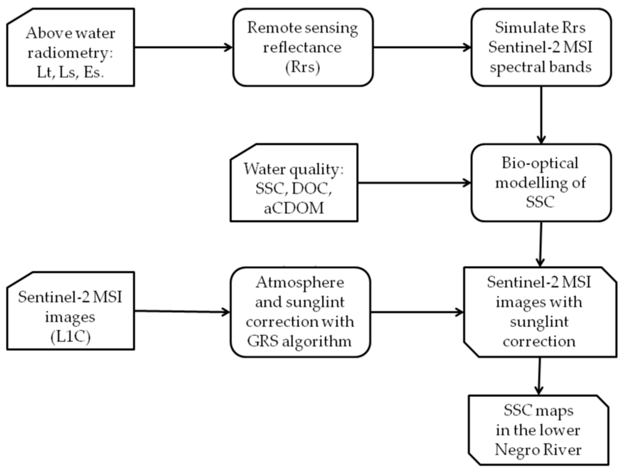
2.3. Models for Estimating SSC

A wide variety of methods are currently available for relating radiometric data with SSC, such as the use of single band [34,36,40], band ratio [18,44,70], semi-analytical methods [33,71], machine learning [72], and artificial neural networks [73]. Previous studies indicate that empirical models that estimate SSC as a function of R_rs in the visible and near-infrared (VNIR) bands perform well in single-band adjusted linear regressions [18,36,42,74] and with the NIR and Red bands ratio [18,38,43].

In this study, we developed empirical models that were based on regression analysis between the SSC and the R_rs. The principal characteristic of inorganic suspended sediment is its large impact on the scattering coefficient and, in turn, the increase of the water-leaving radiance due to their greater refractive index [9,31]. Thus, the regression approach was chosen because the considered SSC values range from low to moderate. For such a range, R_rs increases nearly linearly before reaching asymptotic regime (or “saturation” reflectance) for greater values of SSC, typically >70 mg L⁻¹ [75]. The Orthogonal Distance Regression (ODR) approach [76] was used in addition to the commonly used Ordinary Least Square (OLS) method to better account for the inherent uncertainties of each dataset (R_rs, SSC). The primary advantage of ODR over OLS is its ability to fully take the uncertainty attached to both R_rs and SSC into account [77,78].

The in situ R_rs were analysed as a function of spectral shape and magnitude. Pearson correlation coefficients (r) were calculated to describe the relationship between SSC, DOC, and R_rs, at different wavelengths and as a function of the hydrological period. The spatiotemporal variability of the SSC was analysed by the R_rs, together with the DOC and the water level of the Negro River. This optically active constituent was not considered in this study due to the low concentration of chlorophyll-a from the Negro River (≈1 µg L⁻¹).

The estimates of those uncertainties were assigned to the standard deviation calculated from the several R_rs acquisitions and SSC samples of each station, respectively, as highlighted in the previous section. For each empirical model using the OLS method, the Root Mean Square Error (RMSE, Equation (2)) and Mean Absolute Percentage Error (MAPE, Equation (3)) were used to assess the performance in conjunction with the coefficient of determination (R²).

$$\mathrm{RMSE}= \sqrt{\frac{{\displaystyle \sum }{({\mathrm{x}}_{\mathrm{i}}-{\mathrm{X}}_{\mathrm{obs}})}^2}{\mathrm{n}}}$$

(2)

$$\mathrm{MAPE}= {\displaystyle \sum }_{\mathrm{i}=1}^{\mathrm{n}}\left|\frac{{\mathrm{x}}_{\mathrm{i} -}{\mathrm{x}}_{\mathrm{obs}}}{{\mathrm{x}}_{\mathrm{obs}}}\right|\times 100$$

(3)

where x_obs and x_i are the in situ and estimated SSC values, respectively; n is the number of samples.

2.4. Satellite Data and Processing

A partially cloud-free dataset of Sentinel-2A and Sentinel-2B satellites images acquired during 2017 was used to map the spatial and temporal dynamics of the SSC in the central Anavilhanas Archipelago area (stations RN4, RN5 and LAP in Figure 1). Sentinel-2 MSI data were analysed to quantify performances to remotely monitor anabranching systems that are defined by numerous narrow sections and small ponds that are only accessible through high-resolution satellite data. Note that Sentinel-2 is also well suited for such analyses because of the large number of spectral bands. Available acquisition dates of satellite Sentinel-2 images used in this study can be seen in the Supplementary material Table S1. It was not possible to assess the relationship between water quality data and satellite Sentinel-2 data due to large time lag between satellite and in situ measurements (±10 days).

In situ hyperspectral R_rs was used to simulate the multispectral characteristics of the Sentinel-2 MSI sensor, while taking their specific band widths into account. The reflectance of the Sentinel-2 MSI bands was simulated based on their relative response functions. The simulation of one spectral band consists of applying the relative response functions of the multispectral sensors on the in situ hyperspectral data [69].

Table 1. Spectral characteristics of Sentinel-2 MSI bands used in this study.

Band	Central Wavelength (nm)	Band Width (nm)	Spatial Resolution (m)
3	560	35	10
4	665	30	10
5	705	15	20
6	740	15	20
7	783	20	20
8a	865	20	20

Source: Drusch et al. [80].

presents the spectral configuration of the evaluated bands and the spectral response function of MSI sensor is available at [79]. The Sentinel-2 MSI images with Level-1C (L1C) were accessed from the Copernicus Open Access Hub (https://scihub.copernicus.eu) (accessed on 24 January 2021) that was provided by European Space Agency (ESA).

Sentinel-2 satellite images were frequently contaminated by high sunglint signals (undesired reflection of sunlight on the water surface) due to the low latitude location of the Negro River. Consequently, corrections for the sunglint in addition to the atmosphere itself were mandatory in maximising the number of exploitable images and pixels within those images. For such a purpose, the algorithm GRS, standing for Glint Removal of Sentinel-2-like images [81] was used to fully process the L1C images and provide the spectral values of R_rs.

The GRS algorithm was specifically developed to handle and correct for the direct sunlight reflected by the water surface and potentially reaching the sensor (i.e., sunglint signal) of Sentinel-2 missions, which is, a nadir or near-nadir viewing sensor with Shortwave Infrared (SWIR) bands. The GRS processor consists of three modules to correct for (i) gaseous absorption, (ii) diffuse light from sky and its reflection by the air-water interface, and (iii) the sunglint signal to retrieve the water-leaving signal at the water surface level.

First, the gaseous absorption (mainly CO₂, H₂O and O₃) correction is performed with the SMAC software [82]. For each pixel, the diffuse radiance component is reconstructed for the given viewing geometry (i.e., sensor and Sun viewing angles and relative azimuth) and prescribed aerosol parameter values (i.e., aerosol optical thickness and its spectral dependency) from pre-computed look-up tables (LUT). Atmospheric pressure, gas concentrations, and aerosol parameters are retrieved from bilinear interpolation within the grid of the CAMS dataset [68,83].

The sunglint correction is performed based on an estimation of the bidirectional reflectance distribution function (BRDF) of the rough water surface from the SWIR bands (i.e., ~1610 and ~2200 nm). The sunglint signal that is obtained in the SWIR is then extrapolated toward the NIR and visible bands. The estimation of the sunglint radiance is based on the fact that the water body is virtually totally absorbing; the water absorption coefficient in the SWIR is several orders of magnitude greater than that in the NIR. Once corrected for the atmosphere diffuse radiance, the remaining radiance in the SWIR is interpreted as the pure surface component of the signal and then translated into BRDF. This BRDF in the SWIR is extrapolated to the other bands when considering the spectral variation of the refractive index of water and its important consequences onto the spectral variation of the sunglint signal; see Harmel et al. [81] for details. The water-leaving component at the water surface level is eventually obtained after division by the total transmittance (i.e., diffuse + total transmittances) that is calculated for the bimodal aerosol model from the LUT.

3. Results

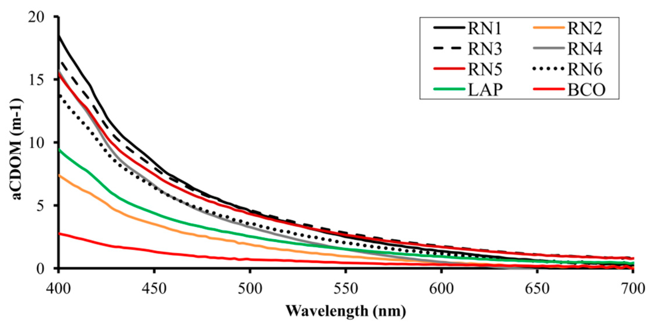
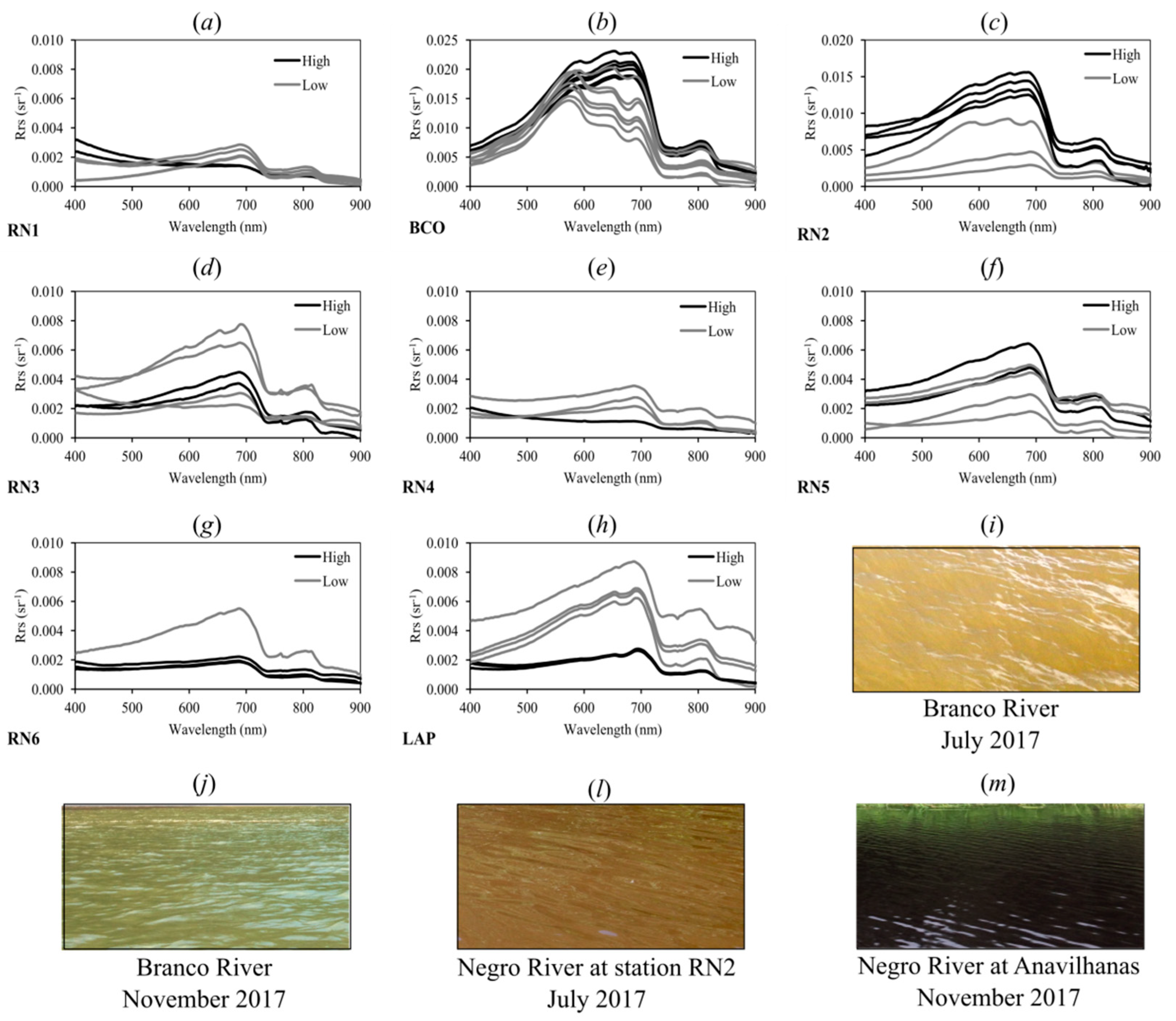
3.1. Water Composition from in situ Data

Table 2. SSC and dissolved organic carbon (DOC) in the Negro and Branco Rivers from 2016 to 2019 (mg L⁻¹).

Sample Station	Location	SSC Mean	SSC Range	DOC Mean	DOC Range
BCO	Branco River	14.70	4.00–22.64	6.98	4.92–9.93
LAP	Apacú Lake at Anavilhanas	5.43	2.39–8.48	8.55	6.47–10.43
RN1	Negro River upstream to Branco River	4.45	2.32–7.61	10.64	9.54–11.26
RN2	Negro River downstream to Branco River	6.18	5.73–11.76	6.48	4.20–10.90
RN3	Negro River upstream to Anavilhanas	3.01	0.44–6.35	10.33	8.51–12.74
RN4	Right bank of the Negro River at Anavilhanas	3.18	0.56–6.15	9.85	8.92–10.73
RN5	Left bank of the Negro River at Anavilhanas	4.02	2.18–6.60	7.41	7.41–10.18
RN6	Negro River downstream to Anavilhanas	1.47	0.48–3.24	8.96	7.58–10.31

summarises the range of measurements of SSC and DOC acquired during the nine field cruises at each sample station along the Negro and Branco Rivers. The Negro River, upstream from the mouth of the Branco River (station RN1), presented an average SSC of 4.45 mg L⁻¹, ranging from 2.32 to 7.61 mg L⁻¹ between the high water and low water periods, respectively. The average SSC of the Branco River near of the mouth was 14.70 mg L⁻¹ with a variation of 4.00 mg L⁻¹ (low water period) to 22.64 mg L⁻¹ (high water period). After confluence with the Branco River, the Negro River at station RN2 presented an increase of SSC (average 6.18 mg L⁻¹) with higher values during the high-water period. In the Anavilhanas Archipelago (stations RN4, RN5 and LAP), the mean SSC was 3.41 mg L⁻¹, with the lowest concentrations being observed in the high-water period.

In the station RN1, the average DOC concentration of Negro River was 10.64 mg L⁻¹, ranging from 9.54 mg L⁻¹ in low water period to 11.26 mg L⁻¹ in high water period. The lowest concentration of DOC was observed in the Branco River during the low water period (4.20 mg L⁻¹), with a mean value of 6.98 mg L⁻¹. Close to the Anavilhanas Archipelago, the mean value of DOC concentration was 9.50 mg L⁻¹ and it ranged from 6.47 mg L⁻¹ (station LAP) to 12.74 mg L⁻¹ (station RN3). The dissolved organic carbon of the Negro River presented small spatiotemporal variability, with a coefficient of variation (CV) of 19%, lower than the suspended sediment (CV = 73%).

Figure 3 shows the variation of light absorption coefficients (aCDOM) for eight samples stations at the Negro and Branco Rivers and a floodplain lake at the Anavilhanas Archipelago. The aCDOM at 440 nm was higher (> 7 m⁻¹) in the stations that are dominated by black water rivers (rich in dissolved organic matter) and lower (< 2 m⁻¹) at the station BCO (a clear water river).

3.2. Relationships between R_rs and Water Quality

Figure 4 presents the in situ R_rs data of the Negro and Branco Rivers during the high and low water period. The shape and magnitude of R_rs have clear differences between both rivers (Figure 4a,b). Despite the low R_rs in the Negro River, spatial and seasonal differences could be observed upstream (Figure 4c,d), inside (Figure 4e–g), and downstream (Figure 4h) of the Anavilhanas Archipelago.

Typical reflectance of the Negro River can be seen in Figure 4a, with R_rs < 0.002 sr⁻¹ across the in situ spectrum of station RN1 with no large variation between the high and low water periods. During the high water period, the in situ R_rs of the Branco River (Figure 4b) presented higher values in the Red band (≈0.020 sr⁻¹ between 640 and 690 nm), while, in the low water period, the R_rs peak was in the green band (≈0.017 sr⁻¹, between 560 and 590 nm). This pattern clearly represents the seasonal variation of the SSC of this river (Table 2). The in situ R_rs of the Branco River showed absorption features at 610 and 675 nm, with a minor peak of R_rs at 810 nm. The Negro River at station RN2 (Figure 4c) presented R_rs with a high intensity in the Red band (between 630 and 700 nm), as a result of the contribution of suspended sediment from the Branco River. Therefore, with higher SSC, the reflectance tends to increase in the direction of longer wavelengths, especially in the Red and NIR bands, thereby modifying the spectral shape of R_rs.

Upstream, inside, and downstream of the Anavilhanas Archipelago (Figure 4d–h), the R_rs show a rapid increase between 500 and 650 nm, followed by a peak at 690 nm, reduction between 700 and 730 nm, and a second peak in 800 nm. These peaks in the Red band have different intensities, with higher values of R_rs being observed upstream of the Anavilhanas (station RN3), in the left bank channel (station RN5), and in Lake Apacú (station LAP), sample stations with higher SSC than observed in station RN4 (Table 2).

The in situ R_rs observed in the Branco River represents an environment with moderate SSC, while the Negro River R_rs represent an environment that is dominated by light absorption due to dissolved organic matter, with reduced reflectance in the visible (between 400 and 760 nm) and a slight increase in NIR (between 760 and 900 nm). Therefore, between the stations BCO and RN6, a reduction of up to 90% in R_rs at 665 nm was observed, which is related to the reduction of SSC in the reach between the mouth of the Rio Branco and upstream from the mouth of the Rio Negro.

We observed that SSC was significantly correlated with DOC (r = −0.68, p < 0.05) (Figure 5). The magnitude of the correlation coefficient was high during the high water level period (r = −0.83, p < 0.05). The SSC was not significantly correlated with DOC (r = −0.52, p > 0.05) in the low water period.

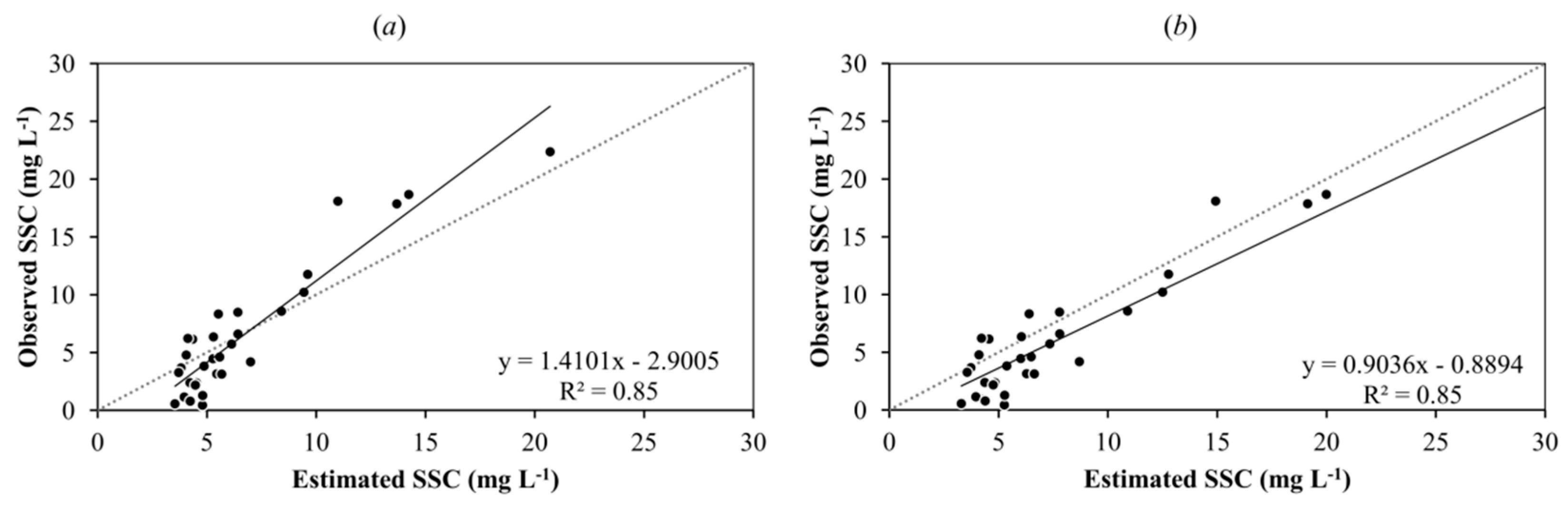
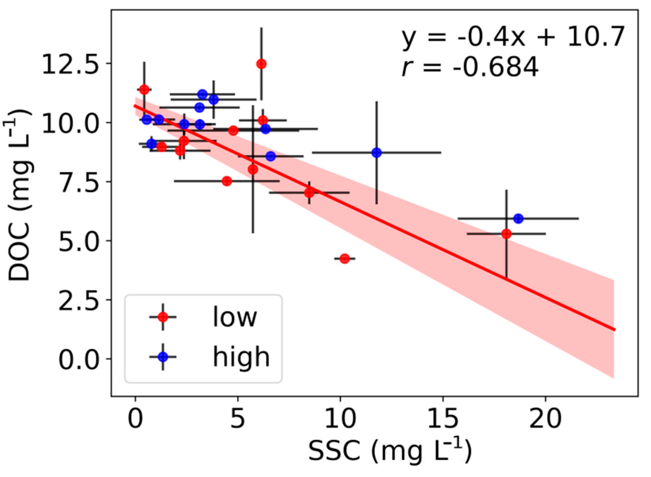
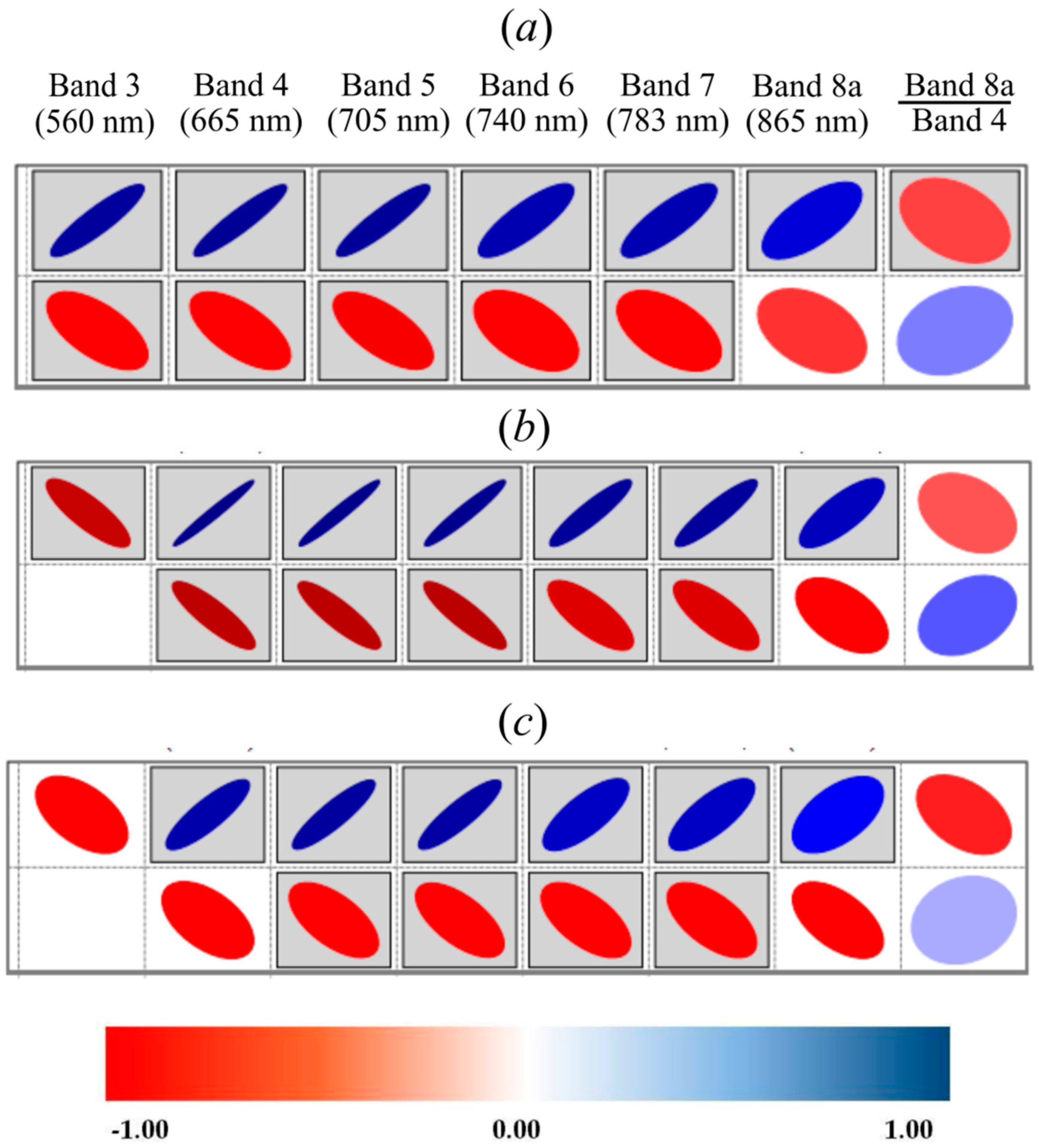
3.2.1. Multispectral MSI Simulated Bands Correlation with SSC and DOC

The Pearson coefficients correlation (r) between SSC and Sentinel-2 MSI simulated bands indicated a positive relationship at different hydrological periods (Figure 6b,c). During the high water period, the correlation was higher, ranging from 0.77 to 0.98 (p < 0.05, Figure 6b). For all of the datasets (low water and high water periods), the r ranged between 0.67 (at 865 nm) and 0.92 (at 665 nm) (Figure 6a).

Conversely, the correlations between DOC and Sentinel-2 MSI simulated bands indicated a negative relationship. During the high water period, the correlation coefficients ranged from −0.75 to −0.87 (p < 0.05, Figure 6b) and, in the low water period, the correlation ranged from −0.60 to −0.64 (p < 0.05, Figure 6c). For all the DOC datasets, the correlation ranged from −0.62 (at 560 nm) to −0.66 (at 705 nm) (Figure 6).

In general, the visible and red-edge bands showed high correlations with SSC while the NIR (Band 8a) and the NIR/Red ratio (Band 8a/Band 4) showed lower correlations. This evaluation indicates that the visible bands have better performance for retrieval SSC of Sentinel-2 MSI data on the Negro River.

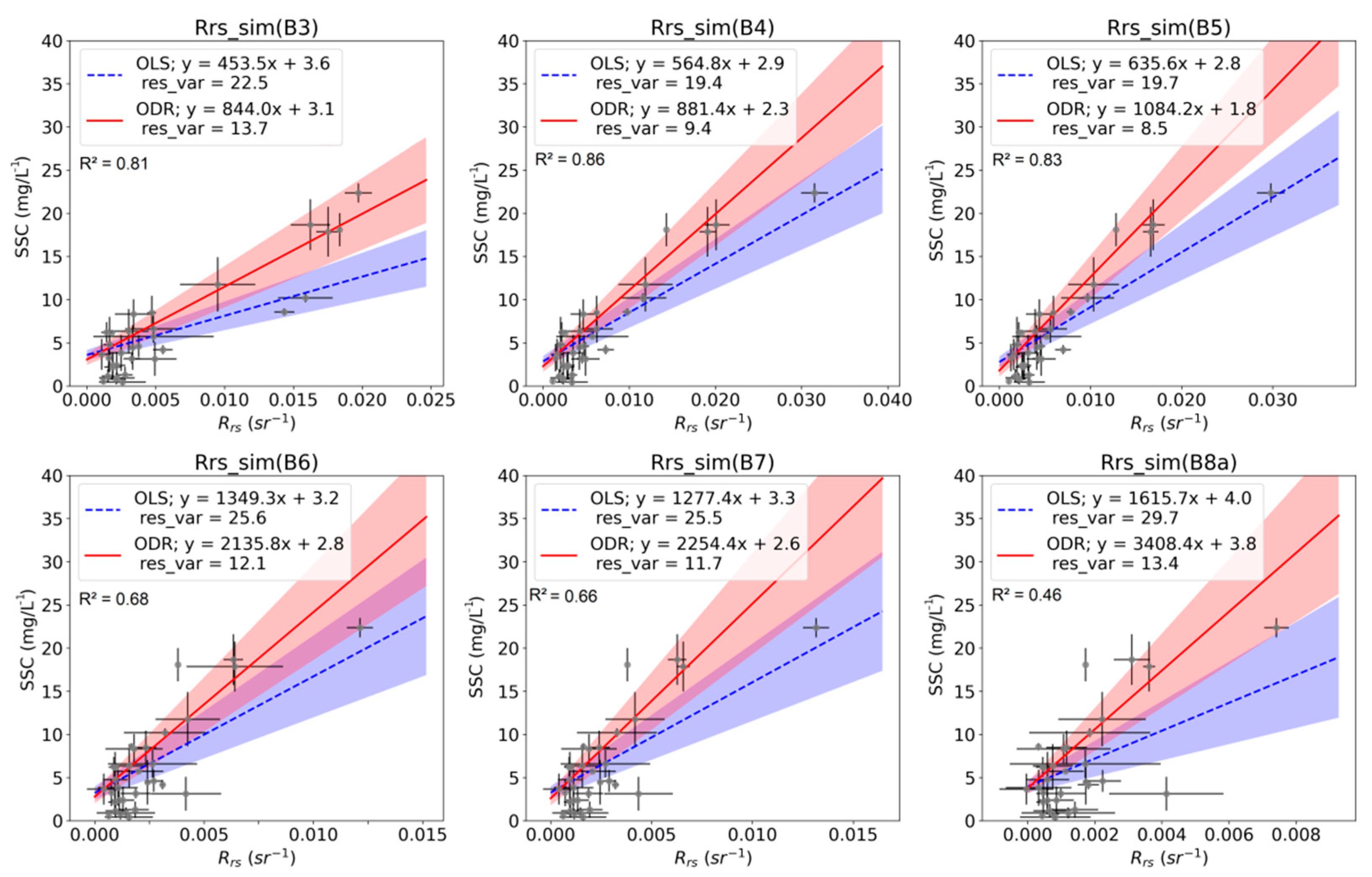
3.2.2. SSC Estimations Based in Sentinel-2 MSI Simulated Bands

Several VNIR Sentinel-2 MSI simulated bands were tested based on the observed correlations (Figure 6), and Figure 7 shows the results of the SSC as a function of R_rs in the lower Negro River basin. Using the OLS method, the models with the best fit were obtained while using simulated band 3 (R_rs at 560 nm) and band 4 (R_rs at 665 nm) of Sentinel-2 MSI (R² > 0.80, RMSE < 1.50 mg L⁻¹ and percentage error < 17%) (

Table 3. Empirical model performance for retrieval SSC using the OLS method.

Sentinel-2 Band	RMSE (mg L−1)	MAPE (%)
Rrs_sim(B3)	1.12	13.20
Rrs_sim(B4)	1.41	16.38
Rrs_sim(B5)	1.53	16.89
Rrs_sim(B6)	1.74	19.45
Rrs_sim(B7)	1.81	19.99
Rrs_sim(B8a)	1.70	18.63
Rrs_sim(B8a)/Rrs_sim(B4)	5.26	61.99

). Good results were also obtained with the band 5 (R² > 0.80, RMSE ≈ 1.50 mg L⁻¹ and percentage error < 17%). The lowest performance was obtained using the ratio of NIR and Red bands (R² < 0.15, RMSE > 5 mg L⁻¹ and percentage error > 60%).

Figure 8 presents the SSC observed versus the SSC derived from Sentinel-2 MSI simulated band 4. It was observed that the SSC derived from simulated band 4 indicated a goodness of fit (R² = 0.86 for OLS and ODR methods) and, for SSC values lower than 6 mg L⁻¹, the OLS method overestimated the observed values. Figure 8 showed that the main advantage of the ODR method was presenting a lower tendency (less-biased slope values) as compared with those that were obtained using the OLS method (decrease 36%, from 1.41 to 0.90). Therefore, it is emphasized that the ODR method (which considers the associated uncertainties) is more suitable than the OLS method for estimating SSC.

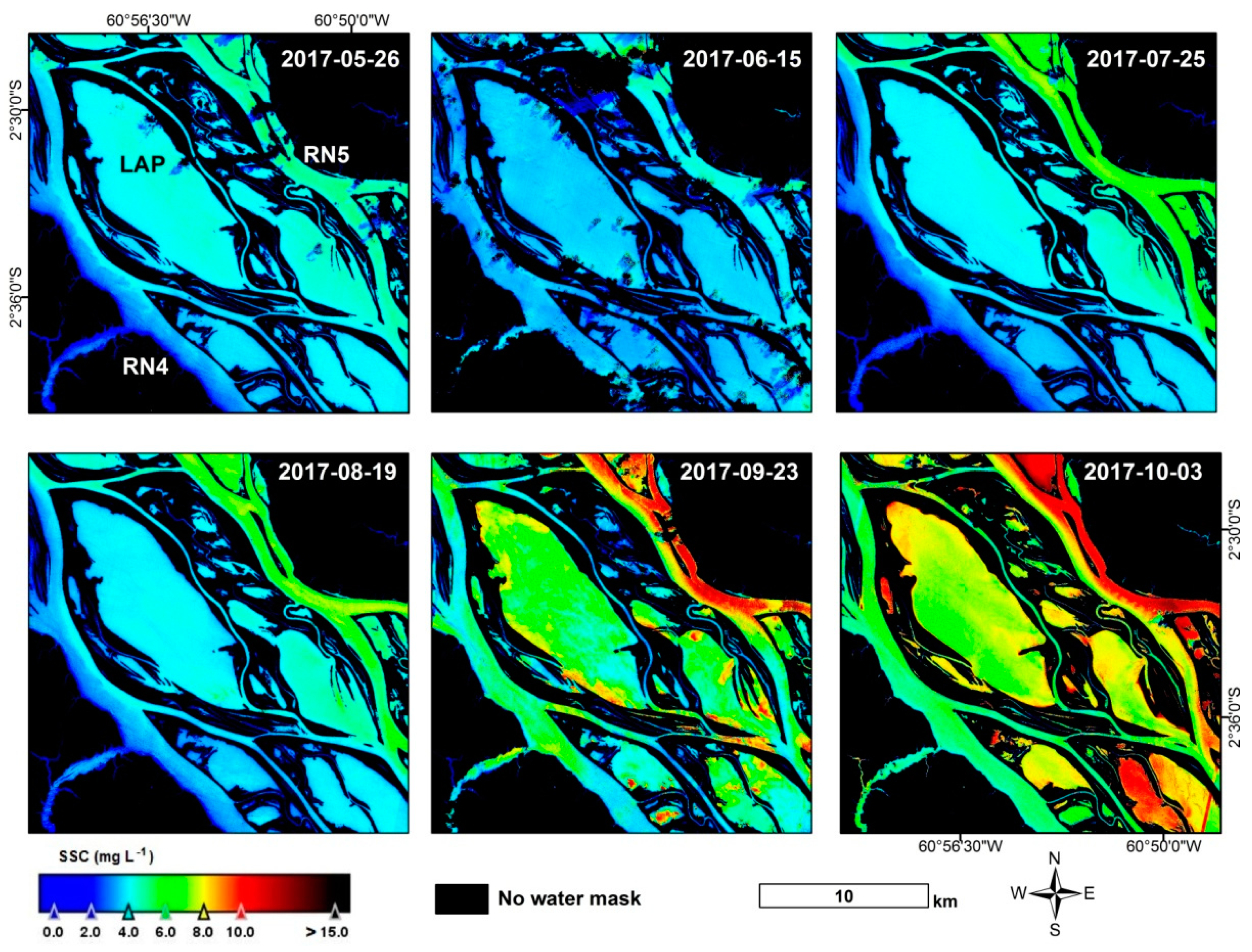
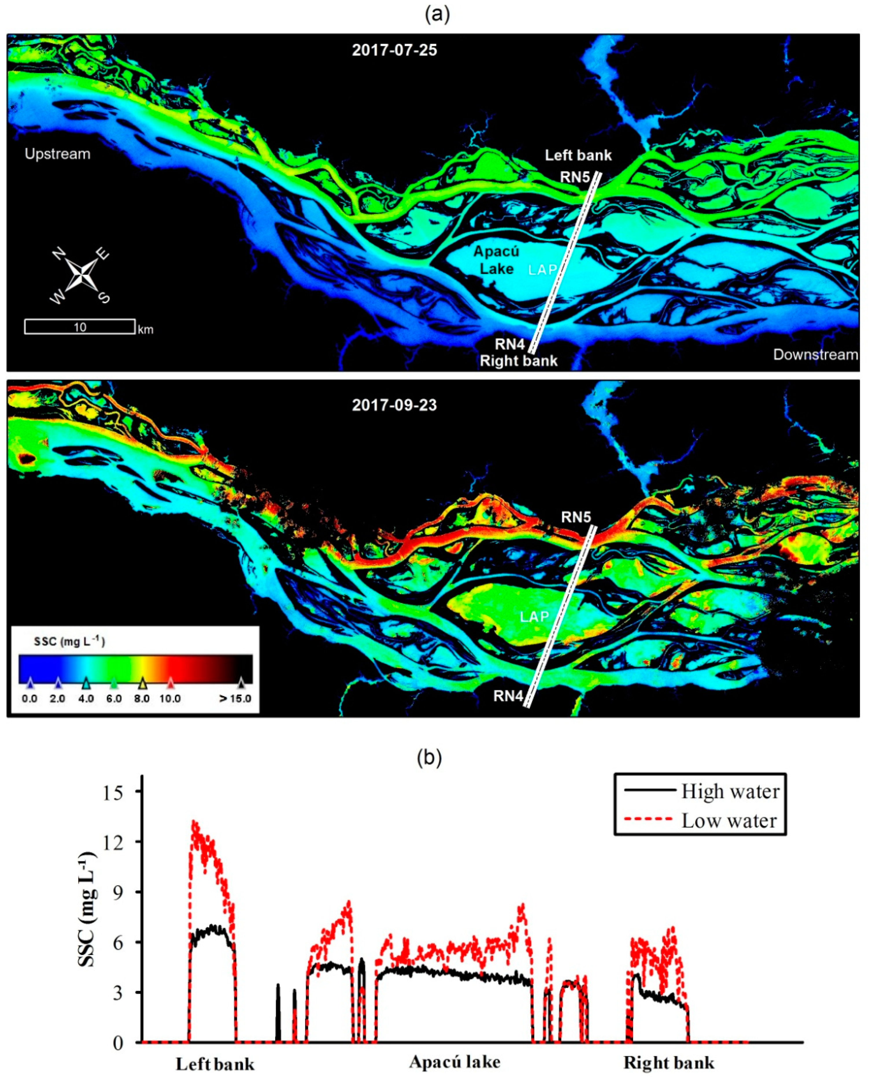
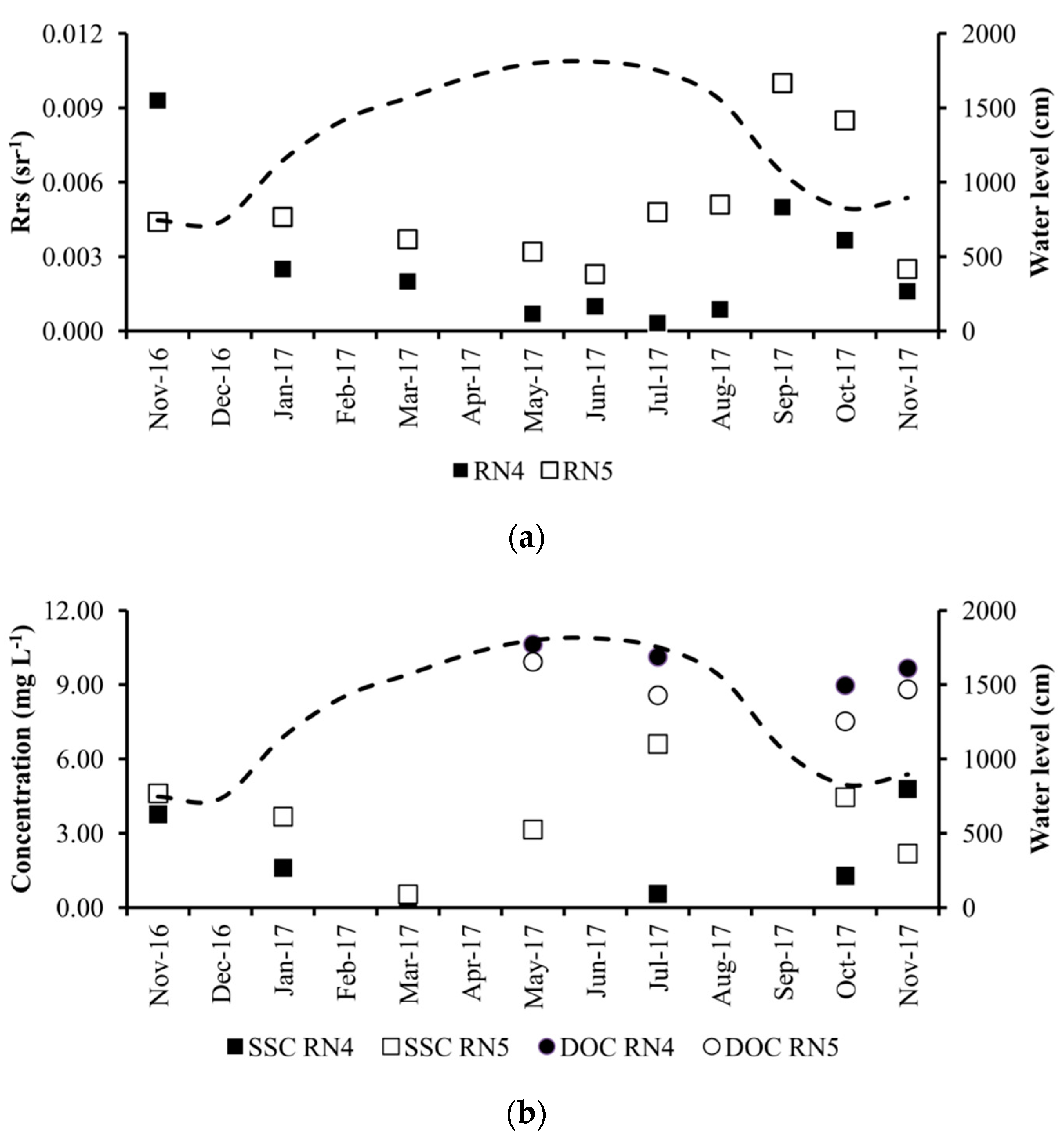
3.3. SSC Spatiotemporal Variability from Satellite Imagery

Inside the Anavilhanas, it was possible to detect a relationship between the R_rs at the Red band (Sentinel-2 MSI band 4) and the water level of the Negro River (Figure 9a). The R_rs at the Red band of station RN4 were progressively lower than that observed in station RN5. This difference may be related to the higher SSC at the station RN5, a region that is influenced by the input of suspended sediments from the Branco River that slightly modifies the Negro River AOPs during the high water period.

At the station RN5, the maximum SSC occurs near the flood peak of the Negro River, while, at station RN4, it was not possible to detect a clear behaviour in the SSC and water level (Figure 9b). Except in the data that were collected during November 2017 (see Figure 9b), the SSC value was greater in the channel on the left bank (station RN5) than the channel on the right bank (station RN4). Conversely, the DOC was always higher in station RN4 as compared to that in station RN5.

The relationship obtained with ODR method using band 4 in Section 3.2.2 was applied to Sentinel-2 MSI images over year 2017. This satellite dataset is used to compare different water levels during the annual cycle. Figure 10 presents the estimated SSC distributions based on Sentinel-2 MSI band 4 images during the rising, high, falling, and low water periods of 2017. In this reach of the Anavilhanas Archipelago, the Negro River has two primary channels and several lakes with different shapes and sizes. The Sentinel-2 MSI band 4 images captured the SSC spatiotemporal variability well. The high detail, the predominance of suspended sediment in the floodplain lakes and channels close to the left bank of the Anavilhanas Archipelago are very noticeable due to the influence of the suspended sediment from Branco River.

Figure 11a shows an overview of the SSC over the Anavilhanas Archipelago in the high and low water periods of the Rio Negro in 2017, highlighting the predominance of higher values close to the left bank of the archipelago. Figure 11b presents the cross profile of SSC between the left and right banks of the Negro River. The difference between the satellite estimates of SSC in the left and right banks were higher than 50% in the high and low water periods.

4. Discussion

4.1. Suspended Sediment Transport in an Anabranching River

The lower Negro River is an old and complex multichannel system due to the presence of the Anavilhanas Archipelago [84], with a very low suspended sediment concentration and under the strong influence of backwater effects of the Amazon River [85]. This hydro-sedimentary behaviour allows for the storage of water and sediments in this archipelago, which are primarily sourced from the Branco River [49]. In the results presented (Table 2), the Negro River downstream from the mouth of the Branco River, (station RN2) in comparison to the upstream sample station (RN1), showed an increase in the SSC of 39%. On the other hand, the mean SSC difference between the sample stations RN2 and RN6 (250 km distance) shows a reduction of 75%, which indicated suspended sediment retention in the Anavilhanas Archipelago. Despite the high volume of water, this sedimentation process is related to the very low velocity of the Negro River (≈0.50 m s⁻¹), the backwater effect from the Amazon River, and the low erosion process in the Anavilhanas Archipelago [49,52].

In the channels of the Negro River without influence of suspended sediment from the Branco River (sample stations RN1, RN4 and RN6 in Figure 10), the low SSC values registered during the high water period could be related to the dilution process that was caused by the larger volume of water available. The hydro-sedimentary dynamics of the Negro River are similar to the process observed at the confluence between the Negro and Amazon rivers [38] and in the Amazon floodplain [86,87].

In the Amazon River and its main tributaries, the concentration of dissolved organic carbon decreases as the concentration of suspended sediment increases, as highlighted by Moreira-Turcq et al. [25]. In the lower Negro River, we observed that SSC was found to correlate inversely with DOC, primarily in the high water period (Figure 5). The water of the Negro River is dominated by dissolved organic matter [23,25] that causes intense light absorption due to coloured dissolved organic matter (CDOM). The Negro River exhibits the higher values of aCDOM when compared to those of Amazon Rivers and its floodplains lakes [46,88] or the reservoirs in the Brazilian semiarid region [89], while demonstrating the same magnitude as those of the Estonian lakes dominated by CDOM [90], as observed in Figure 3.

Even in environments with strong absorption due to CDOM, the results that are presented here (Figure 7) indicate that models with a single spectral band are best suited for water with low suspended sediment concentrations. Previous studies also reported good results for SSC estimation of inland waters using single bands [33,34,36,41,42]. As expected, a higher R_rs in the Negro and Branco Rivers is related to an increase of light scattering by mineral particles [9,18].

In the central area of Anavilhanas (see stations RN4 and RN5 in Figure 1), the water discharge flows through two large channels near to the right and left banks of the archipelago. However, more SSC in the channel on the left bank of the Negro River was observed from in situ (sample station RN5 in Table 2) and Sentinel-2 data (Figure 11a). For example, in the high water period, the difference in suspended sediment discharge between the stations RN4 and RN5 can be over ten times [49]. Inside Anavilhanas Archipelago, the highest amplitude of SSC was observed in the Lake Apacú (station LAP in Table 2), with the minimum and maximum values being obtained during the high and low water periods, respectively. During the low water period, part of the water that was stored in the Anavilhanas lakes throughout the high water period flows to the Negro River channels, and this dynamic may influence the process that increases the concentration of the SSC in some channels and lakes of Anavilhanas Archipelago, as observed in Figure 10 and Figure 11.

Despite the high aCDOM values, the Sentinel-2 MSI data could confirm the spatial heterogeneity of the SSC estimated with in situ R_rs data. During the high and low water periods, the preferred route of suspended sediment inside Anavilhanas can be observed in great detail (Figure 11a). The Sentinel-2 MSI images that were obtained in 2017 allowed for us to see that, even 90 km from its mouth, the suspended sediment from the Branco River influences the R_rs in the Negro River at the Anavilhanas Archipelago, a dynamic that produces differences in the composition of the local fauna and flora [56,91,92]. The SSC cross profile that is retrieved by Sentinel-2 data (see Figure 11b) details this biogeochemical gradient, showing a tendency of reduced suspended sediment concentration between the left bank (station RN5), lakes (station LAP), and right bank (station RN4) of the Anavilhanas Archipelago.

4.2. Use of Passive Satellite Remote Sensing for SSC Monitoring in the Negro River

Multispectral sensors, like Sentinel-2 MSI, were not developed for remote sensing of water; nevertheless, the results here indicate that these spectral configurations are suitable for monitoring SSC in black-water rivers with complex channel pattern, like the Negro River. In this study, the largest percentage error was obtained with the model that uses the NIR and NIR/Red bands ratio, which may be a result of the low NIR response over the Negro River (Table 3). Despite the good performance of the green band (at 560 nm), this band onboard in orbital sensors can be strongly impacted by atmospheric constituents in shorter wavelengths and by sunglint [48,93].

We showed that full consideration of uncertainties attached to the in situ dataset changes the parameterisation of the satellite bands in terms of suspended sediment concentration. A comparison between the OLS (no uncertainty consideration) and ODR methods demonstrated that an estimation of SSC with Sentinel-2 MSI simulated band 4 is less underestimated with the latter (see Figure 8). It is recommended that efforts to fully characterise bias and uncertainties attached to the in situ data and, in particular, for the radiometry measurements are pursued [64,65,66]. The good adjustment that is obtained between SSC and R_rs in the Red band (at 665 nm) is influenced by the presence of suspended sediment from the Branco River.

The lower Negro River is a complex anabranching system with channel width varying from 230 m to 2800 m. Despite this environmental configuration, the Sentinel-2 MSI images thoroughly captured the temporal and spatial variability of the SSC in the Anavilhanas channels and lakes, highlighting, in detail, the predominance of suspended sediments in the lakes and channels near the left bank channel of Anavilhanas.

Although the combination of orbital sensors enables higher temporal resolution [17], the probability of cloud-free imaging in the study area is low throughout a hydrological year [94]. However, multispectral sensors onboard unmanned aerial vehicles can partially overcome these limitations, since they operate at low altitude, and with greater flexibility in revisit time and image acquisition geometry. Conversely, the use of commonly used water-colour sensors with higher temporal resolutions, such MODIS, OLCI, and NPP/VIIRS, allows for us to retrieve a time series of the SSC in the Negro River reaches with channel width >2000 m by using a similar approach that is applied for other large rivers of the Amazon basin [43,44,45,46]. However, the satellite sensors with higher spatial resolutions generally have a greater capacity to detect higher SSC values [95].

The Negro River basin has the lowest coverage in the sediment measurement network that is managed by the Brazilian National Water Agency. Without sedimentometric stations around the Anavilhanas Archipelago, it is difficult to assess temporal variations of the SSC and the relationships between extreme climatic events (El Niño/La Niña) or the temporal variations that will occur due to the Bem Querer dam [96] in the Branco River and subsequently reduce the amount of sediment that arrives in the Anavilhanas Archipelago. The suspended sediment concentration dataset collected in this study before and after they arrive at the archipelago indicate that the Anavilhanas Archipelago retains suspended sediments and acts as sink of fine particles in the lower Negro River (Table 2). Thus, the use of passive satellite data could be an important tool for monitoring suspended sediment transport in areas of great ecological and socioeconomic relevance, such as the Anavilhanas Archipelago.

5. Conclusions

This is the first study that has utilised Sentinel-2 MSI calibrated data for assessing the suspended sediment concentration (SSC) in a large black-water Amazonian river. The waters in the Negro River basin exhibit an absorption budget that is dominated by coloured dissolved organic material. We demonstrated that the so-called black-water rivers, such as the Negro River, exhibit very low suspended sediment concentrations (≈5 mg L⁻¹) and a high coloured dissolved organic material absorption (aCDOM > 7 m⁻¹ at 440 nm). We show that remote sensing reflectance at 665 nm (Red band) can be used in order to monitor suspended sediment concentration in the Negro River with high accuracy (R² > 0.86 and error less than 30% in adjusted models). Thus, passive sensors that are used in satellites operating in the 650–690 nm range can be used to remotely monitor suspended sediment concentrations in this large river. The orthogonal distance regression method demonstrated that estimation of SSC using simulated bands of Sentinel-2 MSI results in less-biased slope values when compared to those obtained using ordinary least square regression.

Our study also highlighted that the suspended sediment from the Branco River causes changes in the apparent optical properties on the low course of Negro River. Indeed, the remote sensing reflectance pattern that was detected with the Sentinel-2 MSI images in the channels and lakes of the Anavilhanas Archipelago was not only similar to the in situ data, but it also showed higher suspended sediment concentration in channels and lakes that were influenced by the Branco River, which is the primary clear water river in the Negro River basin. The suspended sediment transport characterised in this study indicates sedimentation processes in an anabranching reach of the Negro river upstream of the Amazon River.

Therefore, the in situ reflectance dataset from this study contributed to the knowledge of the apparent optical properties in Amazonian rivers. However, further research must be carried out to better assess the inherent optical properties that are based on multispectral and hyperspectral approaches to exploit the full information content of the measured spectra. This will be particularly important for the monitoring of the Negro River basin, including impacts of extreme climate events and potential changes in sediment transport due to deforestation, mining, or the construction of a hydropower dam on this basin.

References

1. Gupta, A. Large Rivers; Gupta, A., Ed.; John Wiley & Sons, Ltd.: Chichester, UK, 2007; ISBN 9780470723722. [Google Scholar]
2. Latrubesse, E.; Stevaux, J.; Sinha, R. Tropical rivers. Geomorphology 2005, 70, 187–206. [Google Scholar] [CrossRef]
3. Allen, P.A. From landscapes into geological history. Nature 2008, 451, 274–276. [Google Scholar] [CrossRef] [Green Version]
4. Bakker, M.M.; Govers, G.; van Doorn, A.; Quetier, F.; Chouvardas, D.; Rounsevell, M. The response of soil erosion and sediment export to land-use change in four areas of Europe: The importance of landscape pattern. Geomorphology 2008, 98, 213–226. [Google Scholar] [CrossRef]
5. Hinderer, M. From gullies to mountain belts: A review of sediment budgets at various scales. Sediment. Geol. 2012, 280, 21–59. [Google Scholar] [CrossRef]
6. Kuhn, C.; de Matos Valerio, A.; Ward, N.; Loken, L.; Sawakuchi, H.O.; Kampel, M.; Richey, J.; Stadler, P.; Crawford, J.; Striegl, R.; et al. Performance of Landsat-8 and Sentinel-2 surface reflectance products for river remote sensing retrievals of chlorophyll-a and turbidity. Remote Sens. Environ. 2019, 224, 104–118. [Google Scholar] [CrossRef] [Green Version]
7. Mouw, C.B.; Greb, S.; Aurin, D.A.; Digiacomo, P.M.; Lee, Z.; Twardowski, M.S.; Binding, C.; Hu, C.; Ma, R.; Moore, T.S.; et al. Aquatic color radiometry remote sensing of coastal and inland waters: Challenges and recommendations for future satellite missions. Remote Sens. Environ. 2015, 160, 15–30. [Google Scholar] [CrossRef]
8. Palmer, S.C.; Kutser, T.; Hunter, P.D. Remote sensing of inland waters: Challenges, progress and future directions. Remote Sens. Environ. 2015, 157, 1–8. [Google Scholar] [CrossRef] [Green Version]
9. Bukata, R.P. Satellite Monitoring of Inland and Coastal Water Quality: Retrospection, Intropection, Future Direction; Taylor & Francis Group: Boca Raton, FL, USA, 2005. [Google Scholar]
10. Gholizadeh, M.H.; Melesse, A.M.; Reddi, L. A Comprehensive review on water quality parameters estimation using remote sensing techniques. Sensors 2016, 16, 1298. [Google Scholar] [CrossRef] [Green Version]
11. Doherty, M. Climate missions to come. In Climate Change & Satellites: Knowledge for Action; Cracknell, G., Calvaud, R., Roca, R., Eds.; Sud[s] Concepts: Paris, France, 2015. [Google Scholar]
12. Agência Nacional de Águas (ANA). HidroSat—Monitoramento Hidrológico por Satélite. Available online: http://hidrosat.ana.gov.br/ (accessed on 29 December 2018).
13. SO-HYBAM. Observation Service SO HYBAM. Available online: http://www.ore-hybam.org (accessed on 29 December 2018).
14. UNESCO. The Unesco-IHP IIWQ World Water Quality Portal. Available online: www.worldwaterquality.org (accessed on 17 April 2020).
15. Crétaux, J.-F. Ocean and inland Waters. In Climate Change & Satellites: Knowledge for action; Cracknell, G., Calvaud, R., Roca, R., Eds.; Sud[s] Concepts: Paris, France, 2015. [Google Scholar]
16. de Lucia Lobo, F.; de Moraes Novo, E.M.L.; Barbosa, C.C.F.; Galvão, L.S. Reference spectra to classify Amazon water types. Int. J. Remote Sens. 2012, 33, 3422–3442. [Google Scholar] [CrossRef]
17. Maciel, D.; Novo, E.; de Carvalho, L.S.; Barbosa, C.; Júnior, R.F.; de Lucia Lobo, F. Retrieving total and inorganic suspended sediments in Amazon floodplain lakes: A multisensor approach. Remote Sens. 2019, 11, 1744. [Google Scholar] [CrossRef] [Green Version]
18. Martinez, J.-M.; Espinoza-Villar, R.; Armijos, E.; Silva Moreira, L. The optical properties of river and floodplain waters in the Amazon River Basin: Implications for satellite-based measurements of suspended particulate matter. J. Geophys. Res. Earth Surf. 2015, 120, 1274–1287. [Google Scholar] [CrossRef]
19. Montanher, O.C.; Novo, E.M.L.M.; Barbosa, C.C.; Rennó, C.D.; Silva, T.S. Empirical models for estimating the suspended sediment concentration in Amazonian white water rivers using Landsat 5/TM. Int. J. Appl. Earth Obs. Geoinf. 2014, 29, 67–77. [Google Scholar] [CrossRef]
20. Pinet, S.; Martinez, J.-M.; Ouillon, S.; Lartiges, B.; Villar, R.E. Variability of apparent and inherent optical properties of sediment-laden waters in large river basins—lessons from in situ measurements and bio-optical modeling. Opt. Express 2017, 25, A283. [Google Scholar] [CrossRef] [PubMed]
21. Gibbs, R.J. The geochemistry of the Amazon River System: Part I. The factors that control the salinity and the composition and concentration of the suspended solids. GSA Bull. 1967, 78, 1203–1232. [Google Scholar] [CrossRef]
22. Leenheer, J.A. Origin and nature of humic substances in the waters of the Amazon River Basin. Acta Amaz. 1980, 10, 513–526. [Google Scholar] [CrossRef] [Green Version]
23. Richey, J.E.; Hedges, J.I.; Devol, A.H.; Quay, P.D.; Victoria, R.; Martinelli, L.; Forsberg, B.R. Biogeochemistry of carbon in the Amazon River. Limnol. Oceanogr. 1990, 35, 352–371. [Google Scholar] [CrossRef]
24. Filizola, N.P. Transfert Sédimentaire Actuel par les Fleuves Amazoniens. Ph.D. Thesis, Paul Sabatier University, Toulouse, France, 2003. [Google Scholar]
25. Moreira-Turcq, P.; Seyler, P.; Guyot, J.L.; Etcheber, H. Exportation of organic carbon from the Amazon River and its main tributaries. Hydrol. Process. 2003, 17, 1329–1344. [Google Scholar] [CrossRef]
26. Abril, G.; Martinez, J.-M.; Artigas, L.F.; Moreira-Turcq, P.; Benedetti, M.F.; Vidal, L.; Meziane, T.; Kim, J.-H.; Bernardes, M.C.; Savoye, N.; et al. Amazon River carbon dioxide outgassing fuelled by wetlands. Nature 2013, 505, 395–398. [Google Scholar] [CrossRef]
27. Filizola, N.; Guyot, J.-L.; Wittmann, H.; Martinez, J.-M.; Oliveira, E. The significance of suspended sediment transport determination on the Amazonian hydrological scenario. In Sediment Transport in Aquatic Environments; InTech: Rijeka, Croatia, 2011; pp. 45–64. [Google Scholar]
28. Latrubesse, E.M.; Arima, E.Y.; Dunne, T.; Park, E.; Baker, V.R.; D’Horta, F.M.; Wight, C.; Wittmann, F.; Zuanon, J.; Baker, P.A.; et al. Damming the rivers of the Amazon basin. Nature 2017, 546, 363–369. [Google Scholar] [CrossRef]
29. Lobo, F.L.; Costa, M.P.F.; Novo, E.M.L.M. Time-series analysis of Landsat-MSS/TM/OLI images over Amazonian waters im-pacted by gold mining activities. Remote Sens. Environ. 2015, 157, 170–184. [Google Scholar] [CrossRef]
30. Winemiller, K.O.; McIntyre, P.B.; Castello, L.; Fluet-Chouinard, E.; Giarrizzo, T.; Nam, S.; Baird, I.G.; Darwall, W.R.T.; Lujan, N.K.; Harrison, I.; et al. Balancing hydropower and biodiversity in the Amazon, Congo, and Mekong. Science 2016, 351, 128–129. [Google Scholar] [CrossRef] [PubMed] [Green Version]
31. Doxaran, D.; Froidefond, J.-M.; Lavender, S.; Castaing, P. Spectral signature of highly turbid waters. Remote Sens. Environ. 2002, 81, 149–161. [Google Scholar] [CrossRef]
32. Mertes, L.A.; Daniel, D.L.; Melack, J.M.; Nelson, B.; Martinelli, L.A.; Forsberg, B.R. Spatial patterns of hydrology, geomorphology, and vegetation on the floodplain of the Amazon river in Brazil from a remote sensing perspective. Geomorphology 1995, 13, 215–232. [Google Scholar] [CrossRef]
33. Nechad, B.; Ruddick, K.G.; Park, Y. Calibration and validation of a generic multisensor algorithm for mapping of total sus-pended matter in turbid waters. Remote Sens. Environ. 2010, 114, 854–866. [Google Scholar] [CrossRef]
34. Novo, E.; Hansom, J.; Curran, P. The effect of viewing geometry and wavelength on the relationship between reflectance and suspended sediment concentration. Int. J. Remote Sens. 1989, 10, 1357–1372. [Google Scholar] [CrossRef]
35. Bernardo, N.; Alcântara, E.; Watanabe, F.; Rodrigues, T.; Imai, N.; Curtarelli, M.; Barbosa, C. Bio-optical model tuning for retrieving the total suspended matter concentration in Barra Bonita reservoir. Rev. Bras. Cartogr. 2015, 67, 1497–1507. [Google Scholar]
36. Chelotti, G.B.; Martinez, J.M.; Roig, H.L.; Olivietti, D. Space-Temporal analysis of suspended sediment in low concentration reservoir by remote sensing. Braz. J. Water Resour. 2019, 24, 1–15. [Google Scholar] [CrossRef] [Green Version]
37. Gallay, M.; Martinez, J.; Allo, S.; Mora, A.; Cochonneau, G.; Gardel, A.; Doudou, J.; Sarrazin, M.; Chow-Toun, F.; Laraque, A. Impact of land degradation from mining activities on the sediment fluxes in two large rivers of French Guiana. Land Degrad. Dev. 2018, 29, 4323–4336. [Google Scholar] [CrossRef]
38. Marinho, T.; Filizola, N.; Martinez, J.-M.; Armijos, E.; Nascimento, A. Suspended sediment variability at the Solimões and Negro confluence between May 2013 and February 2014. Geosciences 2018, 8, 265. [Google Scholar] [CrossRef] [Green Version]
39. Yepez, S.; Laraque, A.; Martinez, J.-M.; De Sa, J.; Carrera, J.M.; Castellanos, B.; Gallay, M.; Lopez, J.L. Retrieval of suspended sediment concentrations using Landsat-8 OLI satellite images in the Orinoco River (Venezuela). Comptes Rendus Geosci. 2018, 350, 20–30. [Google Scholar] [CrossRef]
40. Knaeps, E.; Ruddick, K.; Doxaran, D.; Dogliotti, A.; Nechad, B.; Raymaekers, D.; Sterckx, S. A SWIR based algorithm to retrieve total suspended matter in extremely turbid waters. Remote Sens. Environ. 2015, 168, 66–79. [Google Scholar] [CrossRef] [Green Version]
41. Curran, P.J.; Hansom, J.D.; Plummer, S.E.; Pedley, M.I. Multispectral remote sensing of nearshore suspended sediments: A pilot study. Int. J. Remote Sens. 1987, 8, 103–112. [Google Scholar] [CrossRef]
42. Novoa, S.; Doxaran, D.; Ody, A.; Vanhellemont, Q.; Lafon, V.; Lubac, B.; Gernez, P. Atmospheric corrections and multi-conditional algorithm for multi-sensor remote sensing of suspended particulate matter in low-to-high turbidity levels coastal waters. Remote Sens. 2017, 9, 61. [Google Scholar] [CrossRef] [Green Version]
43. Espinoza-Villar, R.; Martinez, J.-M.; Armijos, E.; Espinoza, J.-C.; Filizola, N.; Dos Santos, A.; Willems, B.; Fraizy, P.; Santini, W.; Vauchel, P. Spatio-temporal monitoring of suspended sediments in the Solimões River (2000–2014). Comptes Rendus Geosci. 2018, 350, 4–12. [Google Scholar] [CrossRef]
44. Espinoza Villar, R.; Martinez, J.-M.; Le Texier, M.; Guyot, J.-L.; Fraizy, P.; Meneses, P.R.; de Oliveira, E. A study of sediment transport in the Madeira River, Brazil, using MODIS remote-sensing images. J. South Am. Earth Sci. 2013, 44, 45–54. [Google Scholar] [CrossRef]
45. Dos Santos, A.L.M.R.; Martinez, J.M.; Filizola, N.P.; Armijos, E.; Alves, L.G.S. Purus River suspended sediment variability and contributions to the Amazon River from satellite data (2000–2015). Comptes Rendus Geosci. 2018, 350, 13–19. [Google Scholar] [CrossRef]
46. Martinez, J.-M.; Guyot, J.; Filizola, N.; Sondag, F. Increase in suspended sediment discharge of the Amazon River assessed by monitoring network and satellite data. Catena 2009, 79, 257–264. [Google Scholar] [CrossRef] [Green Version]
47. Montanher, O.C.; de Moraes Novo, E.M.L.; de Souza Filho, E.E. Temporal trend of the suspended sediment transport of the Amazon River (1984–2016). Hydrol. Sci. J. 2018, 63, 1901–1912. [Google Scholar] [CrossRef]
48. Kutser, T.; Paavel, B.; Verpoorter, C.; Ligi, M.; Soomets, T.; Toming, K.; Casal, G. remote sensing of black lakes and using 810 nm reflectance peak for retrieving water quality parameters of optically complex waters. Remote Sens. 2016, 8, 497. [Google Scholar] [CrossRef]
49. Marinho, R.R.; Filizola Junior, N.P.; Cremon, É.H. Analysis of suspended sediment in the Anavilhanas Archipelago, Rio Negro, Amazon Basin. Water 2020, 12, 1073. [Google Scholar] [CrossRef] [Green Version]
50. Espinoza Villar, R.E.; Martinez, J.-M.; Guyot, J.-L.; Fraizy, P.; Armijos, E.; Crave, A.; Bazán, H.; Vauchel, P.; Lavado, W. The integration of field measurements and satellite observations to determine river solid loads in poorly monitored basins. J. Hydrol. 2012, 444–445, 221–228. [Google Scholar] [CrossRef]
51. Pereira, F.J.S.; Costa, C.A.G.; Foerster, S.; Brosinsky, A.; De Araújo, J.C. Estimation of suspended sediment concentration in an intermittent river using multi-temporal high-resolution satellite imagery. Int. J. Appl. Earth Obs. Geoinf. 2019, 79, 153–161. [Google Scholar] [CrossRef]
52. Latrubesse, E.M.; Stevaux, J.C. The Anavilhanas and Mariuá Archipelagos: Fluvial wonders from the Negro River, Amazon Basin. In Landscapes and Landforms of Brazil; Vieira, B.C., Salgado, A.A.R., Santos, L.J.C., Eds.; Springer: Dordrecht, The Netherlands, 2015; pp. 157–169. [Google Scholar]
53. Filizola, N.; Guyot, J.L. Suspended sediment yields in the Amazon basin: An assessment using the Brazilian national data set. Hydrol. Process. 2009, 23, 3207–3215. [Google Scholar] [CrossRef]
54. Sander, C.; Gasparetto, N.V.L.; dos Santos, M.L.; de Carvalho, T.M. Características do transporte de sedimentos em suspensão na bacia do Rio Branco, Estado de Roraima. Acta Geográfica 2014, 8, 71–85. [Google Scholar]
55. Filizola, N.; Guyot, J.L. Fluxo de sedimentos em suspensão nos rios da Amazônia. Rev. Bras. Geociências 2011, 41, 566–576. [Google Scholar] [CrossRef]
56. Junk, W.J.; Wittmann, F.; Schöngart, J.; Piedade, M.T.F. A classification of the major habitats of Amazonian black-water river floodplains and a comparison with their white-water counterparts. Wetl. Ecol. Manag. 2015, 23, 677–693. [Google Scholar] [CrossRef]
57. Meade, R.H.; Nordin Jr, C.F.; Curtis, W.F.; Rodrigues, F.M.C.; Vale, C.M.D.; Edmond, J.M. Transporte de sedimentos no rio Amazonas. Acta Amaz. 1979, 9, 543–547. [Google Scholar] [CrossRef]
58. Quesada, C.A.; Lloyd, J.; Anderson, L.O.; Fyllas, N.M.; Schwarz, M.; Czimczik, C.I. Soils of Amazonia with particular reference to the RAINFOR sites. Biogeosciences 2011, 8, 1415–1440. [Google Scholar] [CrossRef] [Green Version]
59. Moquet, J.-S.; Guyot, J.-L.; Crave, A.; Viers, J.; Filizola, N.; Martinez, J.-M.; Oliveira, T.C.; Sánchez, L.S.H.; Lagane, C.; Casimiro, W.S.L.; et al. Amazon River dissolved load: Temporal dynamics and annual budget from the Andes to the ocean. Environ. Sci. Pollut. Res. 2015, 23, 11405–11429. [Google Scholar] [CrossRef] [Green Version]
60. Sioli, H. The Amazon and its main affluents: Hydrography, morphology of the river courses, and river types. In Amazon Limnology and Landscape Ecology of Mighty Tropical River and Its Basins; Sioli, H., Ed.; Springer: Dordrecht, The Netherlands, 1984; pp. 127–165. [Google Scholar]
61. Forsberg, B.R.; Devol, A.H.; Richey, J.E.; Martinelli, L.A.; Dos Santos, H. Factors controlling nutrient concentrations in Amazon floodplain lakes. Limnol. Oceanogr. 1988, 33, 41–56. [Google Scholar] [CrossRef]
62. Scofield, V.; Melack, J.M.; Barbosa, P.M.; Amaral, J.H.F.; Forsberg, B.R.; Farjalla, V.F. Carbon dioxide outgassing from Ama-zonian aquatic ecosystems in the Negro River basin. Biogeochemistry 2016, 129, 77–91. [Google Scholar] [CrossRef]
63. Mobley, C.D. Estimation of the remote-sensing reflectance from above-surface measurements. Appl. Opt. 1999, 38, 7442–7455. [Google Scholar] [CrossRef]
64. Zibordi, G.; Voss, K.J.; Johnson, B.C.; Mueller, J.L. Protocols for Satellite Ocean Colour Data Validation: In Situ Optical Radiometry; International Ocean Colour Coordinating Group (IOCCG): Dartmouth, NS, Canada, 2019. [Google Scholar]
65. Harmel, T.; Gilerson, A.; Tonizzo, A.; Chowdhary, J.; Weidemann, A.; Arnone, R.; Ahmed, S. Polarization impacts on the water-leaving radiance retrieval from above-water radiometric measurements. Appl. Opt. 2012, 51, 8324–8340. [Google Scholar] [CrossRef]
66. Gilerson, A.; Carrizo, C.; Foster, R.; Harmel, T. Variability of the reflectance coefficient of skylight from the ocean surface and its implications to ocean color. Opt. Express 2018, 26, 9615–9633. [Google Scholar] [CrossRef]
67. Chami, M.; Lafrance, B.; Fougnie, B.; Chowdhary, J.; Harmel, T.; Waquet, F. OSOAA: A vector radiative transfer model of coupled atmosphere-ocean system for a rough sea surface application to the estimates of the directional variations of the water leaving reflectance to better process multi-angular satellite sensors data over the ocean. Opt. Express 2015, 23, 27829–27852. [Google Scholar] [CrossRef] [Green Version]
68. Morcrette, J.-J.; Boucher, O.; Jones, L.; Salmond, D.; Bechtold, P.; Beljaars, A.; Benedetti, A.; Bonet, A.; Kaiser, J.W.; Razinger, M.; et al. Aerosol analysis and forecast in the European Centre for Medium-Range Weather Forecasts Integrated Forecast System: Forward modeling. J. Geophys. Res. Atmos. 2009, 114, 06206. [Google Scholar] [CrossRef]
69. Lobo, F.L.; Jorge, D.S.F. Processamento de dados, modelagem e mapeamento de parâmetros bio-ópticos. In Introdução ao sensoriamento remoto de sistemas aquáticos. Princípios e aplicações; Barbosa, C.C.F., Novo, E.M.L.M., Martins, V.S., Eds.; Instituto Nacional de Pesquisas Espaciais: São José dos Campos, Brazil, 2019; pp. 82–106. ISBN 978-85-17-00095-9. [Google Scholar]
70. Matthews, M.W. A current review of empirical procedures of remote sensing in inland and near-coastal transitional waters. Int. J. Remote Sens. 2011, 32, 6855–6899. [Google Scholar] [CrossRef]
71. Dorji, P.; Fearns, P.; Broomhall, M. A semi-analytic model for estimating total suspended sediment concentration in turbid coastal waters of Northern Western Australia using MODIS-Aqua 250 m data. Remote Sens. 2016, 8, 556. [Google Scholar] [CrossRef] [Green Version]
72. Peterson, K.T.; Sagan, V.; Sidike, P.; Cox, A.L.; Martinez, M. Suspended sediment concentration estimation from landsat imagery along the Lower Missouri and Middle Mississippi rivers using an extreme learning machine. Remote Sens. 2018, 10, 1503. [Google Scholar] [CrossRef] [Green Version]
73. Sari, V.; dos Reis Castro, N.M.; Pedrollo, O.C. Estimate of suspended sediment concentration from monitored data of tur-bidity and water level using artificial neural networks. Water Resour. Manag. 2017, 31, 4909–4923. [Google Scholar] [CrossRef]
74. Papoutsa, C.; Retalis, A.; Toulios, L.; Hadjimitsis, D.G. Defining the Landsat TM/ETM+ and CHRIS/PROBA spectral regions in which turbidity can be retrieved in inland waterbodies using field spectroscopy. Int. J. Remote Sens. 2014, 35, 1674–1692. [Google Scholar] [CrossRef]
75. Luo, Y.; Doxaran, D.; Ruddick, K.; Shen, F.; Gentili, B.; Yan, L.; Huang, H. Saturation of water reflectance in extremely turbid media based on field measurements, satellite data and bio-optical modelling. Opt. Express 2018, 26, 10435–10451. [Google Scholar] [CrossRef] [Green Version]
76. Boggs, P.T.; Byrd, R.H.; Rogers, J.E.; Schnabel, R.B. User’s Reference Guide for ODRPACK Version 2.01; U.S. Department of Commerce: Gaithersburg, MD, USA, 1992.
77. Mikkonen, S.; Pitkänen, M.R.A.; Nieminen, T.; Lipponen, A.; Isokääntä, S.; Arola, A.; Lehtinen, K.E.J. Technical note: Effects of uncertainties and number of data points on line fitting—A case study on new particle formation. Atmos. Chem. Phys. Discuss. 2019, 19, 12531–12543. [Google Scholar] [CrossRef] [Green Version]
78. Volpe, V.; Silvestri, S.; Marani, M. Remote sensing retrieval of suspended sediment concentration in shallow waters. Remote Sens. Environ. 2011, 115, 44–54. [Google Scholar] [CrossRef]
79. ESA. Sentinel-2 Spectral Response Functions (S2-SRF). Available online: https://sentinel.esa.int/web/sentinel/user-guides/sentinel-2-msi/document-library/-/asset_publisher/Wk0TKajiISaR/content/sentinel-2a-spectral-responses (accessed on 24 January 2021).
80. Drusch, M.; Del Bello, U.; Carlier, S.; Colin, O.; Fernandez, V.; Gascon, F.; Hoersch, B.; Isola, C.; Laberinti, P.; Martimort, P.; et al. Sentinel-2: ESA’s optical high-resolution mission for GMES opera-tional services. Remote Sens. Environ. 2012, 120, 25–36. [Google Scholar] [CrossRef]
81. Harmel, T.; Chami, M.; Tormos, T.; Reynaud, N.; Danis, P.-A. Sunglint correction of the Multi-Spectral Instrument (MSI)-SENTINEL-2 imagery over inland and sea waters from SWIR bands. Remote Sens. Environ. 2018, 204, 308–321. [Google Scholar] [CrossRef]
82. Rahman, H.; Dedieu, G. SMAC: A simplified method for the atmospheric correction of satellite measurements in the solar spectrum. Int. J. Remote Sens. 1994, 15, 123–143. [Google Scholar] [CrossRef]
83. Benedetti, A.; Morcrette, J.-J.; Boucher, O.; Dethof, A.; Engelen, R.J.; Fisher, M.; Flentje, H.; Huneeus, N.; Jones, L.; Kaiser, J.W.; et al. Aerosol analysis and forecast in the European Centre for Medium-Range Weather Forecasts Integrated Forecast System: 2. Data assimilation. J. Geophys. Res. Atmos. 2009, 114, D13205. [Google Scholar] [CrossRef] [Green Version]
84. Latrubesse, E.M. Patterns of anabranching channels: The ultimate end-member adjustment of mega rivers. Geomorphology 2008, 101, 130–145. [Google Scholar] [CrossRef]
85. Meade, R.H.; Rayol, J.M.; Da Conceicão, S.C.; Natividade, J.R.G. Backwater effects in the Amazon River basin of Brazil. Environ. Geol. Water Sci. 1991, 18, 105–114. [Google Scholar] [CrossRef]
86. Fassoni-Andrade, A.C.; de Paiva, R.C.D. Mapping spatial-temporal sediment dynamics of river-floodplains in the Amazon. Remote Sens. Environ. 2019, 221, 94–107. [Google Scholar] [CrossRef]
87. Park, E.; Latrubesse, E.M. Modeling suspended sediment distribution patterns of the Amazon River using MODIS data. Remote Sens. Environ. 2014, 147, 232–242. [Google Scholar] [CrossRef]
88. Da Silva, M.P.; Sander De Carvalho, L.A.; Novo, E.; Jorge, D.S.F.; Barbosa, C.C.F. Use of optical absorption indices to assess seasonal variability of dissolved organic matter in Amazon floodplain lakes. Biogeosciences 2020, 17, 5355–5364. [Google Scholar] [CrossRef]
89. Coelho, C.; Heim, B.; Foerster, S.; Brosinsky, A.; De Araújo, J.C. In situ and satellite observation of CDOM and chlorophyll-a dynamics in small water surface reservoirs in the Brazilian semiarid region. Water 2017, 9, 913. [Google Scholar] [CrossRef] [Green Version]
90. Kutser, T.; Casal Pascual, G.; Barbosa, C.; Paavel, B.; Ferreira, R.; Carvalho, L.; Toming, K. Mapping inland water carbon content with Landsat 8 data. Int. J. Remote Sens. 2016, 37, 2950–2961. [Google Scholar] [CrossRef]
91. Montero, J.C.; Latrubesse, E.M. The igapó of the Negro River in central Amazonia: Linking late-successional inundation forest with fluvial geomorphology. J. South Am. Earth Sci. 2013, 46, 137–149. [Google Scholar] [CrossRef]
92. Scabin, A.B.; Costa, F.R.C.; Schöngart, J. The spatial distribution of illegal logging in the Anavilhanas archipelago (Central Amazonia) and logging impacts on species. Environ. Conserv. 2011, 39, 111–121. [Google Scholar] [CrossRef]
93. Martins, V.S.; Barbosa, C.C.F.; Carvalho, L.A.S.; Jorge, D.S.F.; Lobo, F.D.L.; Novo, E.M.L.M. Assessment of atmospheric correction methods for Sentinel-2 MSI images applied to amazon floodplain lakes. Remote Sens. 2017, 9, 322. [Google Scholar] [CrossRef] [Green Version]
94. Asner, G.P. Cloud cover in Landsat observations of the Brazilian Amazon. Int. J. Remote Sens. 2001, 22, 3855–3862. [Google Scholar] [CrossRef]
95. Dorji, P.; Fearns, P. Impact of the spatial resolution of satellite remote sensing sensors in the quantification of total suspended sediment concentration: A case study in turbid waters of Northern Western Australia. PLoS ONE 2017, 12, e0175042. [Google Scholar] [CrossRef] [PubMed]
96. EPE. Usina Hidrelétrica (UHE) Bem Querer. Available online: http://www.uhebemquerer.com.br/ (accessed on 11 December 2018).
Figure 1. (a) Study area and the sampled stations on a 300 km reach of the Negro River. (Sentinel-2 Multi-Spectral Instrument (MSI) image RGB 11-8a-4). (b) Water level of the Negro River at Manaus Fluviometric station (black line) between July-2016 and March-2020. Dots indicate the date of in situ data collection.
Ijgi 10 00086 g001
Figure 2. The methodology used for modelling the suspended sediment concentration (SSC) with in situ Rrs and the application in the Sentinel-2 MSI images.
Ijgi 10 00086 g002
Figure 3. Absorption coefficients of coloured dissolved organic matter (CDOM) of the Negro and Branco Rivers, and Apacú Lake at Anavilhanas Archipelago.
Ijgi 10 00086 g003
Figure 4. In situ Rrs of the high (black line) and low water period (grey line) of the Negro (a,c–g) and Branco (b) Rivers and of floodplain lake at Anavilhanas Archipelago (h). Water colours variability in the study area (i–m). Note: y-axis of stations BCO and RN2 is different from that of samples stations in the Negro River.
Ijgi 10 00086 g004
Figure 5. Relationship between DOC and SSC including low water period (red) and high water (blue) period. The shaded areas indicate the uncertainty.
Ijgi 10 00086 g005
Figure 6. Correlogram maps of SSC (upper rows), DOC (lower rows) and Sentinel-2 MSI simulated bands with in situ Rrs (columns): (a) All dataset. (b) For the high water period. (c) For the low water period. Significant Pearson correlation coefficients (p < 0.05) are showed in grey boxes. Blue colours correspond to positive correlations and red colours correspond to negative correlations. The ellipses forms reflect the high and low magnitude of the Pearson correlation coefficient.
Ijgi 10 00086 g006
Figure 7. Empirical models between SSC and Rrs for Green (B3), Red (B4, B5, B6, and B7) and NIR (B8a) Sentinel-2 MSI simulated bands using Orthogonal Distance Regression (ODR) and Ordinary Least Square (OLS). The shaded areas indicate the uncertainty. For the ratio B8a/B4 see supplementary Figure S1.
Ijgi 10 00086 g007
Figure 8. Comparison of SSC observed and estimated using in situ Rrs Sentinel-2 MSI simulated band 4 with OLS (a) and ODR (b) methods. The dashed line indicates values 1:1. For the other Sentinel-2 MSI simulated bands see Supplementary Figure S2.
Ijgi 10 00086 g008
Figure 9. Variability of Rrs at 665 nm (Sentinel-2 MSI band 4) and water level (dashed line) of the Negro River in 2017 (a). For the Sentinel-2 MSI other bands see supplementary Figure S3. Variability of SSC, DOC, and water level (dashed line) of the Negro River in 2017 (b).
Ijgi 10 00086 g009
Figure 10. Spatial and temporal variability of SSC between May and October 2017 in the central reach of Anavilhanas Archipelago.
Ijgi 10 00086 g010
Figure 11. Spatial distribution of satellite-retrieved mean SSC on 7/25/2017 (high water) and 9/23/2017 (low water) in the Anavilhanas central reach (a). Cross profile of SSC between left and right banks (b).
Ijgi 10 00086 g011