A Unified Methodology for the Generalisation of the Geometry of Features

Abstract

The development of generalisation (simplification) methods for the geometry of features in digital cartography in most cases involves the improvement of existing algorithms without their validation with respect to the similarity of feature geometry before and after the process. It also consists of the assessment of results from the algorithms, i.e., characteristics that are indispensable for automatic generalisation. The preparation of a fully automatic generalisation for spatial data requires certain standards, as well as unique and verifiable algorithms for particular groups of features. This enables cartographers to draw features from these databases to be used directly on the maps. As a result, collected data and their generalised unique counterparts at various scales should constitute standardised sets, as well as their updating procedures. This paper proposes a solution which consists in contractive self-mapping (contractor for scale s = 1) that fulfils the assumptions of the Banach fixed-point theorem. The method of generalisation of feature geometry that uses the contractive self-mapping approach is well justified due to the fact that a single update of source data can be applied to all scales simultaneously. Feature data at every scale s < 1 are generalised through contractive mapping, which leads to a unique solution. Further generalisation of the feature is carried out on larger scale spatial data (not necessarily source data), which reduces the time and cost of the new elaboration. The main part of this article is the theoretical presentation of objectifying the complex process of the generalisation of the geometry of a feature. The use of the inherent characteristics of metric spaces, narrowing mappings, Lipschitz and Cauchy conditions, Salishchev measures, and Banach theorems ensure the uniqueness of the generalisation process. Their application to generalisation makes this process objective, as it ensures that there is a single solution for portraying the generalised features at each scale. The present study is dedicated to researchers concerned with the theory of cartography.

1. Introduction

The development of methods of generalising (simplifying) a geometry object in digital cartography involves, for the most part, the improvement of existing algorithms, and also the disregarding of mathematical objectivity in the verification of the geometry of figures before and after the process, i.e., the features necessary for the automatic generalisation of the object [1,2,3,4,5,6,7,8]. Currently, a big challenge for automatic digital generalisation in multi-resolution databases (MRDB) [9] involves increasing the scope of use and the searching of data collected in such a way (which is related to database queries and geo-visualisation) [10,11,12].

One of the basic tasks of the MRDB, especially in the geodata databases maintained by the state cartographic services, is the harmonisation of data obtained from other databases [13,14]. This makes it necessary to establish constant “cartographic control points in MRDBs” [9,15]. The overriding goal set by the UN-GGIM (United Nations Committee of Experts on Global Geospatial Information Management) for state mapping services is the interoperability of databases. The condition for fulfilling this task is the development of generalisation algorithms, free from the subjective decision of the authors [8,15,16].

The development of a fully automatic generalisation method for the entire spatial database (Digital Landscape Model) [17,18,19] and for the cartographic portrayal of this database (Digital Cartographic Model) [20,21,22,23] calls for algorithms that are clearly verifiable for a particular group of objects. This will allow cartographers from the aforementioned bases to choose any objects. This follows from the aforementioned needs that once-acquired data and their unambiguous, objective generalisation at various scales are the requirements for the INSPIRE (INfrastructure for SPatial InfoRmation in Europe) directive [24] for the purposes of database harmonisation and interoperability.

The paper presents a new solution for digital automatic cartographic generalisation for the geometry of linear and areal objects. It uses the properties of contractive self-mapping, which in a strict mathematical manner allows the source data of the object belonging to the metric space to be clearly mapped and verified. At scales s <1 of polygonal generalisations—${ł}_u$, there is one objective mapping result if the mapping data meet the properties of the metric space—L_m, as well as the following additional conditions:

• The necessary condition: the Lipschitz condition (contraction), i.e., p > h, and the Banach theorem in the shrinking projection for TG [12,25] are preserved in each envelope with the sequences of points on the polyline—the contractive mapping with the participation of the binary tree system for the considered triangles:;
• The sufficient conditions of:

  (a)

  Cauchy’s criterion [25] in the contractive mapping at the scale—s < 1,

  (b)

  Minimum dimensions according to, e.g., A. Salishchev [26]: bases—p and heights of triangles TK of the generalised line;

  (c)

  The verification of the rejected dimensions for source line points.

2. Metric Space

Metric space is a set with an imposed metric, i.e., with a function that defines the distance between any two members of the set. Metric spaces are the most general class of sets, which use the concept of distance—patterned on the distance known from Euclidean spaces (line, plane, three-dimensional space) [27].

In each envelope, the ordered polyline is transformed with a contractive mapping and fulfils the necessary and sufficient conditions in polyline generalisation. Also needs to have objective result for scales s < 1, dependent only on scale s. This is confirmed by the test results (Figure A8 and Figure A9) and in line with the Banach theorem [12,27]. Furthermore, the generalisation of the geometry of objects, which is one of the three reefs of mapping established by E. von Sydow in 1857 [1], following the procedure giving here, is no longer a reef due to the fact that it has one objective solution at every scale.

In digital cartographic generalisation, the continuity of the sequence of points in intervals of this space, as well as their sum, mean that there is only one objective result. Moreover, the generated information has an increased degree of credibility.

For the purposes of digital cartography, the linear and areal objects of a metric space are sequences of points describing the geometry of natural and man-made objects. The data of these objects require ordering for their processing, in accordance with the rules of the Lm metric space, which in turn is a generalisation of the properties of Euclidean space. Thanks to the requirements of the said space, the results of the digital cartographic generalisation can be seen to be objective, which leads to an increase in the degree of the credibility of the generated information.

Cartographic Control of Linear and Areal Objects in a Metric Space

Cartographic Control of Linear and Areal Objects in a Metric Space [25]. Cartographic control base (OKO) consists of fixed points of the base, distinguished by the properties of the object’s location, shape and dimensions. The determination of them allows their temporal exclusion from the process in order to preserve their invariance in contraction mapping (contractor). In multiresolution databases (MDRB), the selection of OKO improves the scope of application of these databases and the range of the data search within them (which is connected with inquiries and geo-visualisation) [10].

OKO is made up of the following objects:

• Natural:

  (a)

  Open linear, represented by sequences of fixed points, the beginning and end of which define one axis of the local coordinate system,

  (b)

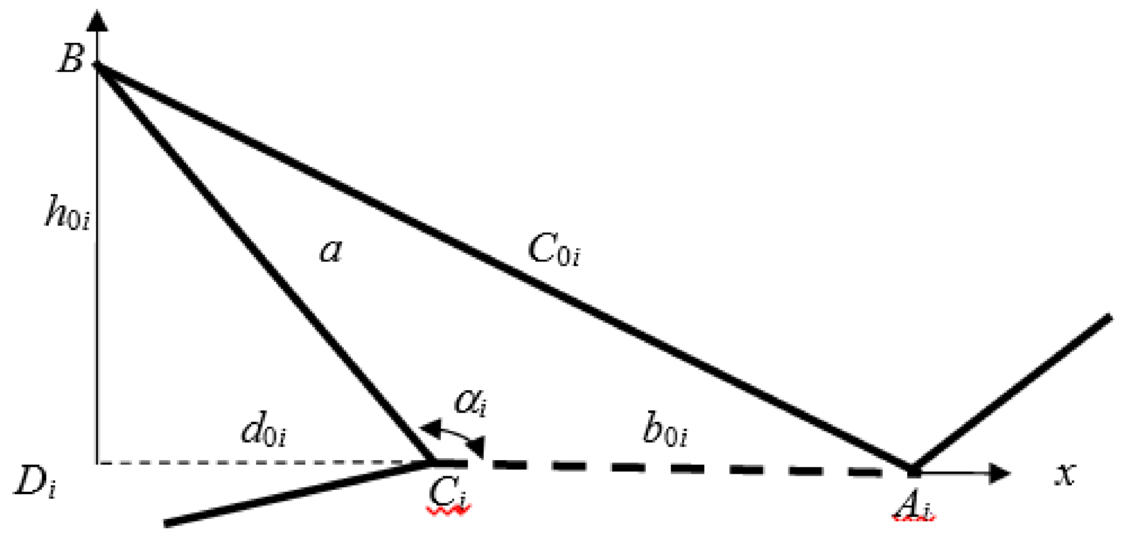
  Areal or base objects, the outline of which is divided into two parts, creating triangles with a common base. The common base has a maximal length (Figure 1), which assures the preservation of the contraction condition when mapping polyline envelopes.

• Snthropogenic:

  (a)

  Buildings, linear objects (roads, engineered rivers) and areal objects.

Points belonging to the anthropogenic objects within OKO are determined in a similar way to those of a natural object, i.e., with their beginning and end singled out.

In order to maintain the stability of the Cartographic Control, the Cartographic Control of an Object OKO attribute in meta-data of MDRB bases should be determined automatically only once, by a national mapping agency (NMA). In metric space $L_z$, if OKO points are not excluded from the mapping, substantial distortions of the produced map may occur.

3. Definitions and Notations

Three types of triangles are considered in the paper:

TB—base triangles, constructed by object points in different coordinate systems transformed into one geodetic system. These triangles constitute the base for the creation of initial contraction triangles TK (Figure 2) from their left and right edge. Characteristic features of these triangles are their bases, which are simultaneously the longest sides of triangles TK, as they extend from the beginning to the end in every interval.

TK—contraction triangles built within the envelopes of the polyline:

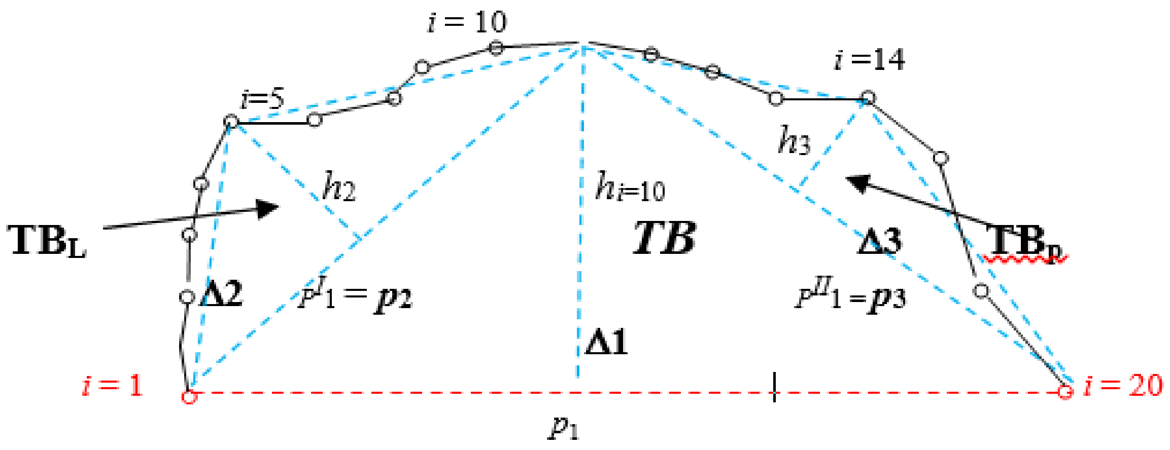
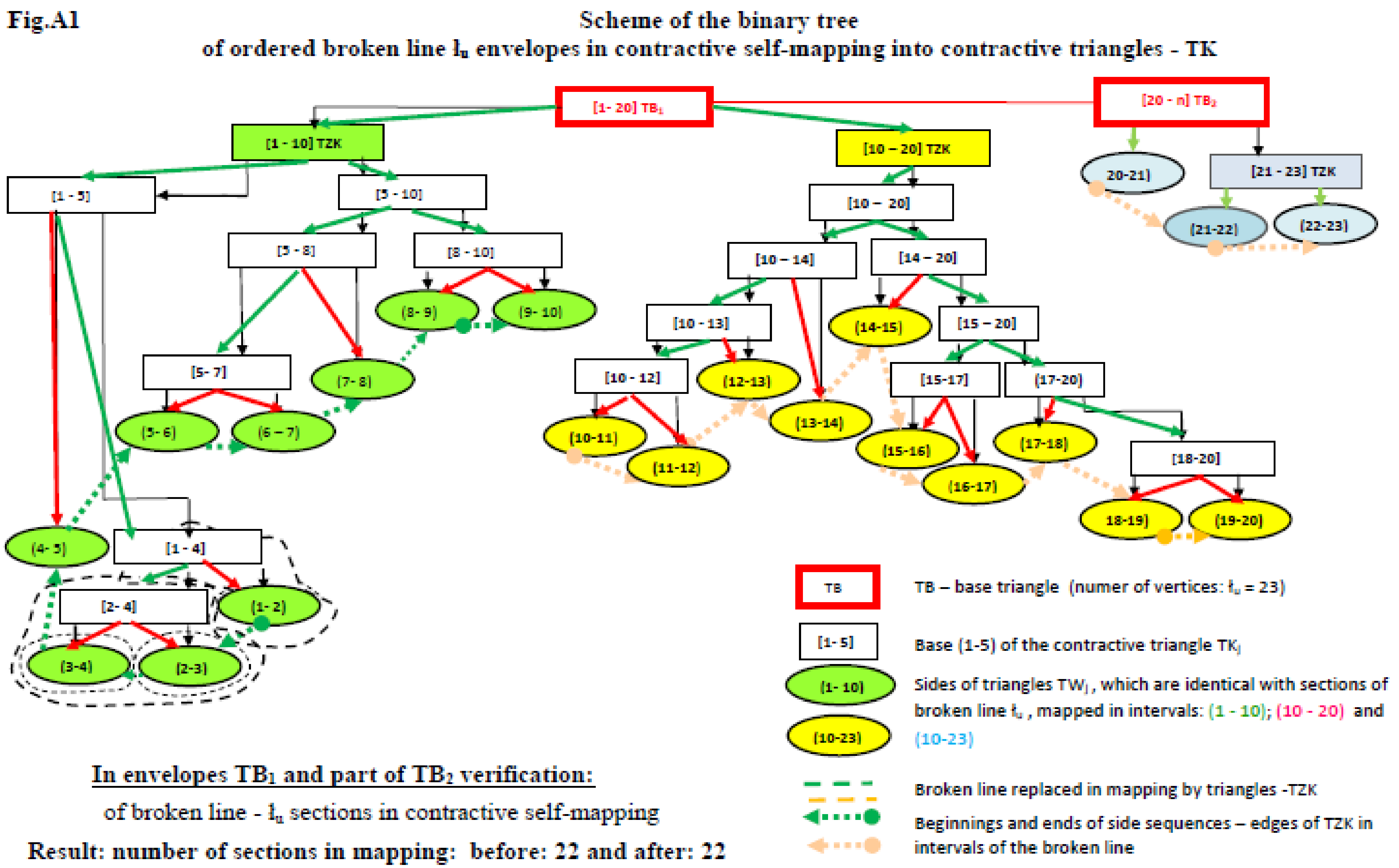
• The first triangle TK in every envelope of the polyline in the contractive self-mapping which has the longest base and fulfils condition (2),
• Consecutive triangles TK which have (a) common side(s) and are constructed according to the binary tree scheme. Their sides are shorter than those of preceding triangles, which results from the assumption of the base TB on the longest section connecting cartographic control points of the areal object,
• The procedure of the contractive self-mapping ends with the triangle TG.

TG—limiting triangle TK of the contractive self-mapping of polyline envelopes into contraction triangles; in TG, at least one side is a section of the source—the ordered polyline ${ł}_u$.

The following notations are used in the paper:

• ${ł}_u$ = ordered polyline, i.e., continuous sequences of points in closed intervals, with nodes;
• i = 1, 2, 3, …, n,
• j = 1, 2, 3, …, k—numbers of triangles—envelopes, built of segments of the polyline;
• α_j—Lipschitz constant (of contraction);
• (X, ρ_X)—metric space with metric ρ_X;
• f—contraction mapping $f:X\to X$, the images of which are triangles TK.

Contraction triangles TK_j form an irregular grid on segments, or envelopes, of the polyline. The grid arises from the base triangle TB according to the scheme of the data binary tree (Figure 2). Contraction triangles TK_j are images of a contraction mapping operator, and are under the following assumptions:

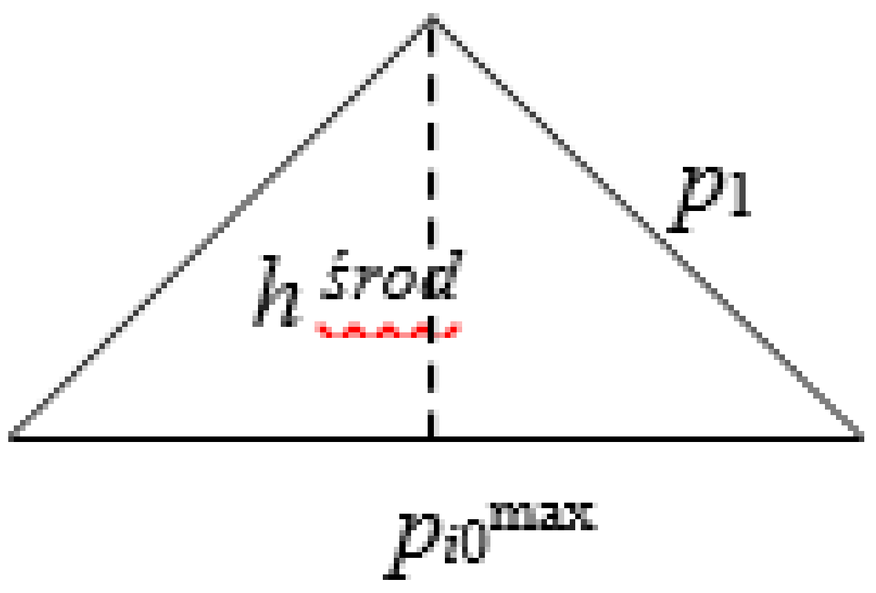
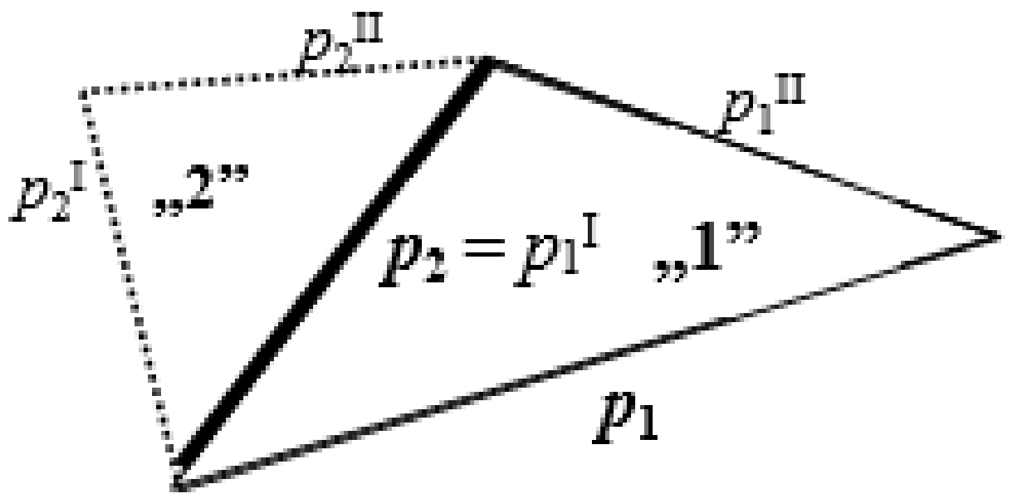
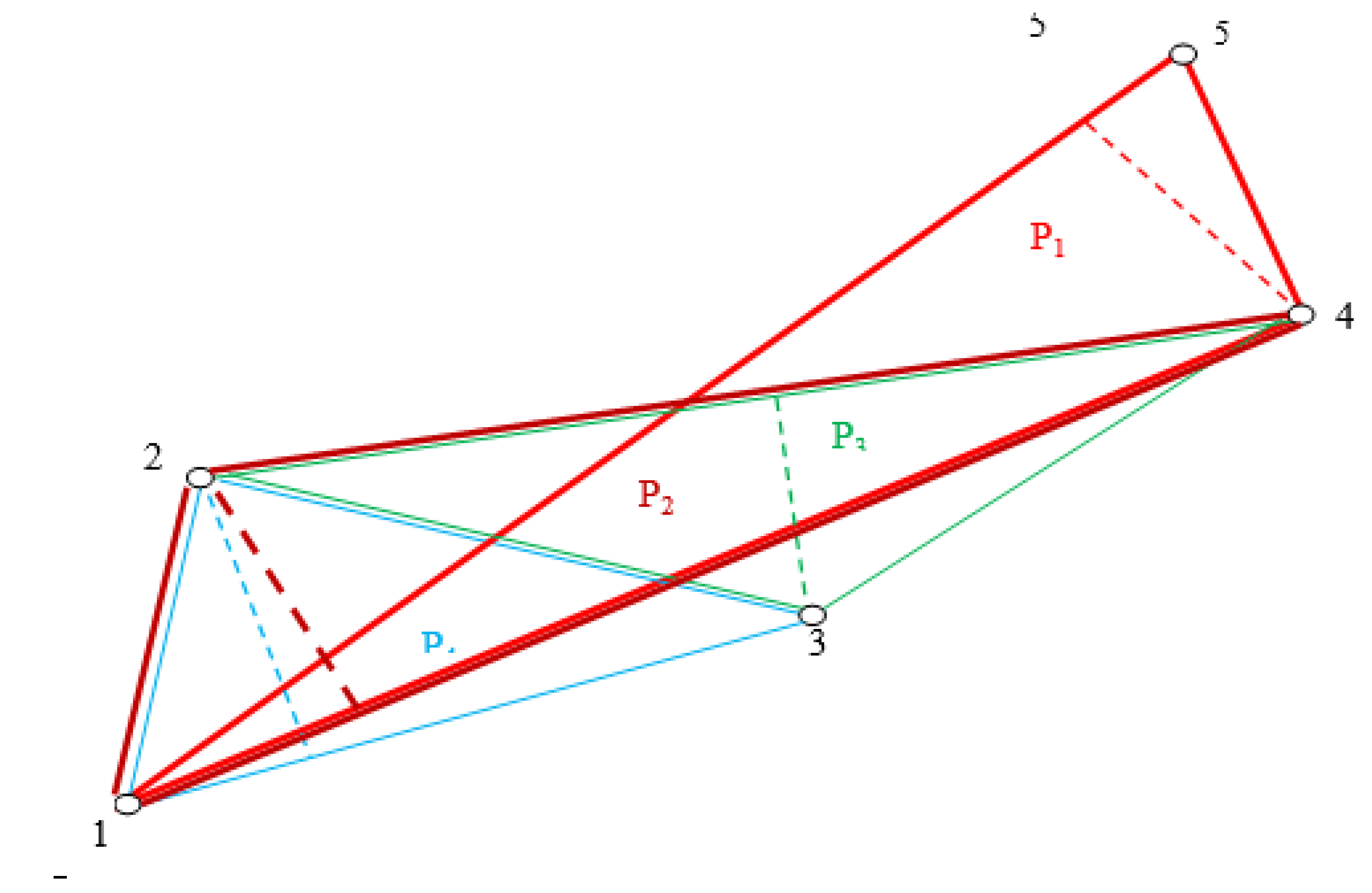
• Triangle sides (edges) are oriented clockwise—when observed from its base (Figure 2);
• In a triangle, for j = 1 (TK₁), with base p₁, sides are marked as:

  (b)

  left: p^I₁,

  (c)

  right: p^II_1,

• Consecutive envelopes of the polyline are created according to the binary tree scheme in the form of two triangles with sides:

  (a)

  bases: left p₂ and right p₃,

  (b)

  sides: left: p^I₂; p^I₃ and right: p^II₂; p^II₃.

In addition, OKO elements for generalisation are the points of the polyline that determine the contractive triangles TK in envelopes (Figure 2), the bases of which are greater than the heights.

Triangles TK are created in the envelopes (hulls) of the polyline as consecutive iterations of the contractive self-mapping; they are built on the edges of the triangles, which are sections of an ordered polyline. In Figure 2, polyline ${ł}_u$ consists of points i = 1–20. As an example, a sequence of envelopes of polyline ${ł}_u$ is created by the sections between nodes (1–5); (5–10); (10–14); (14–20), which constitute a consecutive iteration of a binary tree construction in the form of triangles.

The following definition explains the contractive mapping ([26], p. 203):

Contraction, or contractive mapping, is a projection f of metric space $\left(X,\rho x\right)$ into metric space $\left(Y,\rho y\right)$, for which there exists real constant $a\in (0,1)$ so that for arbitrary $x_1,x_2\in X$ the inequality ${\rho }_Y(\left(f\left(x_1\right),f\left(x_2\right)\right)\le a·{\rho }_X\left(x_1,x_2\right)$. is fulfilled.

For the needs of this paper, contractive mapping f is defined in such a way that it transforms an ordered polyline ${ł}_u$ of geographic data into the binary tree structure of contractive triangles TK. Therefore, ${ł}_u\subset D_f$ and $f\left({ł}_u\right)=\left\{T{K}_j\right\}$, which means that f maps a sequence of sections within the envelope of the ordered polyline ${ł}_u$ into a set of TK, and the mapping is unique:

$$f:{ł}_u\to f\left({ł}_u\right)$$

(1)

4. The Necessary and Sufficient Conditions for the Contractive Mapping in Digital Generalisation Process

The introduction of contractive mappings to digital generalisation yields unique objective results of the process. It can be achieved, provided certain conditions are imposed on data and one-way mappings.

In digital generalisation, one strives to eliminate the inconclusiveness of its results. Polylines ${ł}_u$ contain points (nodes) which cause inconsistencies in results [8] [Chrobak et al. 2015], and which were named singular points. They can be found through triangles created on polyline ${ł}_u$ from its consecutive three points. The bases of these triangles (which do not belong to the polyline) form a single axis of a local orthogonal coordinate system. Their geometry is verified by condition (2), from which it uniquely results that the longest side of the examined triangle is its base, which in turn fulfils Equation (3). The positive result of the verification of condition (2) allows for the examination of the remaining triangles of the polyline. If condition (3) is not fulfilled by the lengths of the examined triangle, the vertex positioned opposite to the side determining the axis of local coordinate system is a singular point. The identification of the singular points of the examined polyline allows for:

(a)

The exclusion of these points from the mapping procedure by setting them limits of intervals;

(b)

The preservation of the continuity, repeatability and uniqueness of mapping;

Ad. (a) Fulfilment of condition (2) assures that every created triangle TK has a base longer than its other sides (Figure 3). Its vertex becomes a singular point when one or both sides are longer than the base. The triangle is then defined as in Figure 4, with condition (3);

Ad. (b) In self-mapping, triangles TK preserve condition (2) and the intervals of the polyline are composed of continuous sequences of points. Their continuity assures that the contractive self-mapping of an ordered polyline fulfils the contraction condition and the Banach theorem on unique solutions. The solution is the original polyline (created before mapping) and, thanks to that, the mapping is repeatable.

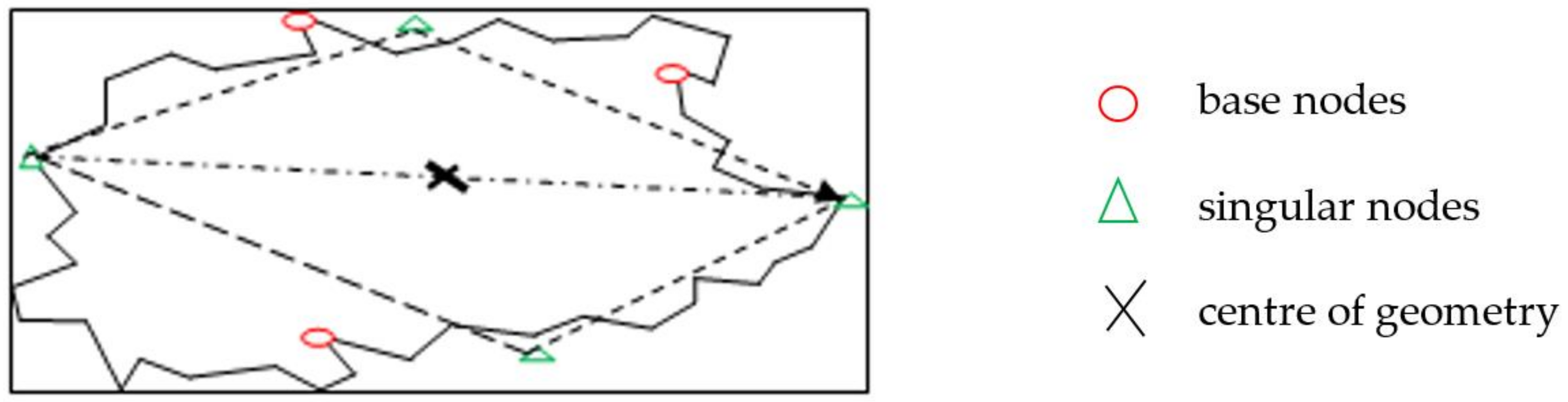
Determination of Singular Points—Nodes of Polyline ${ł}_u$ in Metric Space $L_z$

The determination of singular points on the polyline is achieved by the sequential creation of triangles from its three consecutive points. Moreover, the bases of these triangles do not belong to the line. In these triangles (Figure 3), their dimensions are verified by condition (2), which highlights the singular point or vertex positioned opposite the base and fulfilling condition (3).

$$p_{i,j}^{max}>h_{i,j}^{środ} \mathrm{and} h^{środ}<\frac{\sqrt{n^2-1}}{2}{p}_0$$

(2)

i = 1, 2, 3, …, m (nodes of the polyline)

j = 1, 2, 3, …, k (contractive triangles TK)

n—number dividing base p of triangle TK, if abscissa of height h is not in the middle of base p (n = 2, 3, 4, …, w)

$$h^{środ}<\frac{\sqrt{3}}{2}{p}_0$$

When n = 2, condition (2) confirms that every base p₀ of triangle TK is longer than its height.

A local coordinate system is created in every triangle of the polyline under examination. In a triangle for which condition (2) is not fulfilled, the longest side is determined by Equation (3):

$$\begin{gathered} {\left(c_{0i}^{roz}\right)}^2=h_{0i}^2+{\left(b_{0i}+d_{0i}\right)}^2 \\ {H}_{0i}^2=a_i^2-d_{0i}^2 \end{gathered}$$

and hence

$$\begin{gathered} {\left(c_{oi}^{roz}\right)}^2=a_i^2-d_{0i}^2+{\left(b_{0i}+d_{0i}\right)}^2=a_i^2+b_{0i}^2+2b_{0i}{d}_{0i} \\ {c}_{0i}^{roz}=\sqrt{a_i^2+b_{0i}^2+2b_{0i}{d}_{0i}} \end{gathered}$$

(3)

5. Contractive Self-Mapping of Ordered Polyline (Segmented Line) ${ł}_u$

In metric space $\left(X,\rho \right)$, images in contractive self-mapping $f:X\to X$ of polyline ${ł}_u$, envelopes, built on geographic data and possessing the structure of a binary tree (Figure A1), while triangles TK (Figure A2) fulfil condition (2).

The polyline is split into envelopes whose borders are marked by the singular points in accordance with Equation (3) and create sections of the polyline. The base triangles TBs, the vertices of which are the beginning and end points of the polyline ${ł}_u$ forming triangles TB, which are created in these sections of the polyline ${ł}_u$ (Figure 2). The edges TB_L and TB_P (Figure 2) determine the points of the limit of the section, connecting the beginning-to-middle edge TB_L with the middle-to-end-of-the-section edge TB_P. Within the envelopes, the binary tree system triangles are created on polyline ${ł}_u$. The first triangle TK—the beginning one (of each envelope polyline)—determines the length limit between the beginning and end points of the TB_L edge, which is the base of the first triangle TK. The remaining edge TB_P of the base triangle TB is determined in the same manner (Figure 2).

The contractive self-mapping has an application in the geometry of open figures, and the closed ones are separated into two base triangles TB (Figure 1) with a common base. The singular points of the polyline ${ł}_u$ are temporarily excluded from the mapping. The triangles TKj in the envelopes are created by a top–down approach, with inequality (2) being maintained. Each triangle TK (consecutive in iteration) has a common side with its neighbour.

The experience gained from the examination of the currently used algorithms for digital cartographic generalisation, mentioned at the beginning of the paper, calls for their broader application complemented by contractive self-mapping, fulfilling the contraction condition at arbitrary scale s ≤ 1. The generalisation of every linear object is well justified [8]. Contractive self-mapping has the following properties:

• An unequivocal and user independent result;
• Verification of contractive self-mapping of an ordered polyline ${ł}_u$ result by its original data;
• Preservation of the similarity condition of the polyline by original points in contractive mappings at scales s < 1, which according to the Cauchy condition and minimum dimensions of Salishchev (so univocally) are not removed at a given scale.

Research on the application of contractive self-mapping for the digital generalisation of linear objects at scales s ≤ 1 point out that it can become a standard of such generalisation (Figure A3). They led to the formulation of the following thesis:

In metric space (X, ρ), the f: X → X contractive self-mapping of the ordered polyline ${ł}_u$ into triangles TK with a binary tree structure, is created if the Lipschitz condition is preserved, and if its result is objective and independent from the user at all scales of the generalisation.

Proof: 

bases p₁ and p₂ of triangles TK are determined in the binary tree structure through self-mapping with the preservation of the following assumptions for the neighbouring triangles  □

• Each pair of neighbouring triangles of polyline ${ł}_u$, of two consecutive iterations of their construction, has a common side,
• In the envelope of the polyline ${ł}_u$, the length of the base of each created triangle TK is greater than the length of its edges, which is guaranteed by condition (2).

Fulfilling the assumptions means that p₁ > p₂, since the common edge of triangles “1” and “2” $p_2=p_1^I$ (Figure 5) is shorter than base $p_1$, but longer than edge $p_2^I$ of the triangle “2” of which it is the base.

In this way, triangles TK are created according to the binary tree structure, with the preservation of the Lipschitz contraction condition, in the form of:

$$\left|f\left(p_1\right)-f\left(p_2\right)\right|=\left|p_1^I-p_2^I\right|\le a\left|p_1-p_2\right|$$

(4)

Considering the boundary case where $p_1^I=p_2^I=p$, which means that triangle “2” is equilateral (Figure 6), we obtain:

$$p^2=h^2+{\left(\frac{p}{2}\right)}^2$$

(5)

From which: $h=\frac{\sqrt{3}}{2}p$, $0.866p\ge h>0$

In other words, $p>h$, which fulfils condition that is given by Formula (2).

Relation (4) can then be written as

$$\left|f\left(p_1\right)-f\left(p_2\right)\right|=\left|p_1^I-p_2^I\right|=0\le a\left|p_1-p_2\right|$$

(6)

Dividing both sides of inequality (6) by α and $p_1$, we obtain $0\le 1-\frac{p_2}{p_1}$, and then $\frac{p_2}{p_1}\le 1$.

In each contractive mapping, the base of triangle “1” is longer than its sides, which is reflected by the inequality.

In the binary tree system, each iteration of two neighbouring triangles that have a common side of contractive mapping fulfils the condition $\alpha =\frac{p_2}{p_1}<1$. In the section of polyline ${ł}_u$ of each binary tree, the iteration of a sequence of triangles TK of unidirectional contractive mapping fulfils the condition of α <1. This is due to the fact that the limits of the polyline section are triangles that follow the mentioned rules: the first with the maximum possible length of its sides and the end-of-the-section boundary triangle with the minimum lengths of the triangle TK edges create the lengths of the sides of the source polyline ${ł}_u$. The binary tree interactions of TK triangles are continuous in the section (because α < 1), which results in the contraction condition being fulfilled in each section of the polyline ${ł}_u$. Moreover, the mapping-preserving contractions of the polyline ${ł}_u$ belong to the metric space in its sections, so the summation of the partial generalisations in the sections of the polyline ${ł}_u$ is the result of the mapping. Thus, the usefulness of the required and sufficient conditions in contractive self-mapping has been proven to be necessary to obtain an objective result in digital generalisation at each scale.

The extreme case of an equilateral triangle was included in the examination of the contraction condition for the contractive triangles of a polyline (Figure 5). If the triangle fulfils condition (2), it preserves the condition of the contractive self-mapping of polyline envelopes. In summary, triangles TK created in the envelopes of the polyline according to the binary tree scheme (Figure 5) maintain the properties of contractive self-mapping. This is because in the case of two TK triangles having common side, the Lipschitz condition (4) with constant α < 1 is fulfilled.

Values α are not stable within the procedure of contractive mapping of triangles contained in the polyline ${ł}_u$ envelopes (Figure A8, col. 10). In every iteration of the mapping, the “local constant” assumes another value from the interval 0 < α < 1. This is due to the irregular structure of polyline sections processed into triangles TK. Therefore α changes but does not exceed the value of 1 (which is caused by the fulfilment of condition (2)). The contractive self-mapping preserves the contraction condition, and is unidirectionally continuous, repeatable and possesses a unique solution: the source data of the polyline.

The second task of the contractive mapping of a polyline ${ł}_u$ at scales s < 1 is to improve the self-mapping for scales used in arbitrary generalisations of the line. This would yield at every scale s < 1, due to self-mapping and the properties of its continuity and repeatability preservation, a unique (one) result. Such mapping would cause a unique removal of points undistinguishable at a given scale, which would not preserve the Cauchy condition with Salishchev’s minimum dimensions (Figure A3).

Figure 7 presents part of the polyline ${ł}_u$, which illustrates the fulfilment of contraction condition (4) for mapping, with local constant α < 1. Section 1, Section 2, Section 3, Section 4 and Section 5 is the base of base triangle TB (1-4-5). On its edge 1–4, and by fulfilling condition (2) of the tree system, triangles TK with decreasing lengths of their bases are formed according to the binary tree system and variable mapping scales. Relations between the sides of the constructed triangles are shown in column C of

Table 1. Results proving the Lipschitz condition for constant α < 1 in the contractive mapping of a polyline.

No TKj	TK	Base pj	Left Edge pjI	Right Edge pjII	Relations	α = pj+1/pj
A	B				C	D
1	1-4-5	p1 = 1-5	pI4-5	pII1-4	p1 > pII1-4 = p2	0 < p2/p1 < 1
2	1-2-4	p2 = 1-4	pI1-2	pII2-4	p2 > pII2-4 = p3	0 < p3/p2 < 1
3	2-3-4	p3 = 2-4	pI3-4	pII2-3	p3 > pII2-3 = p4	0 < p4/p3 < 1
4	1-2-3	p4 = 2-3	pI1-3	pII2-1	p4 > pI1-3 p4 > pII2-1	0 < α < 1

, while the contractive character of the local mappings is confirmed by the results shown in column D.

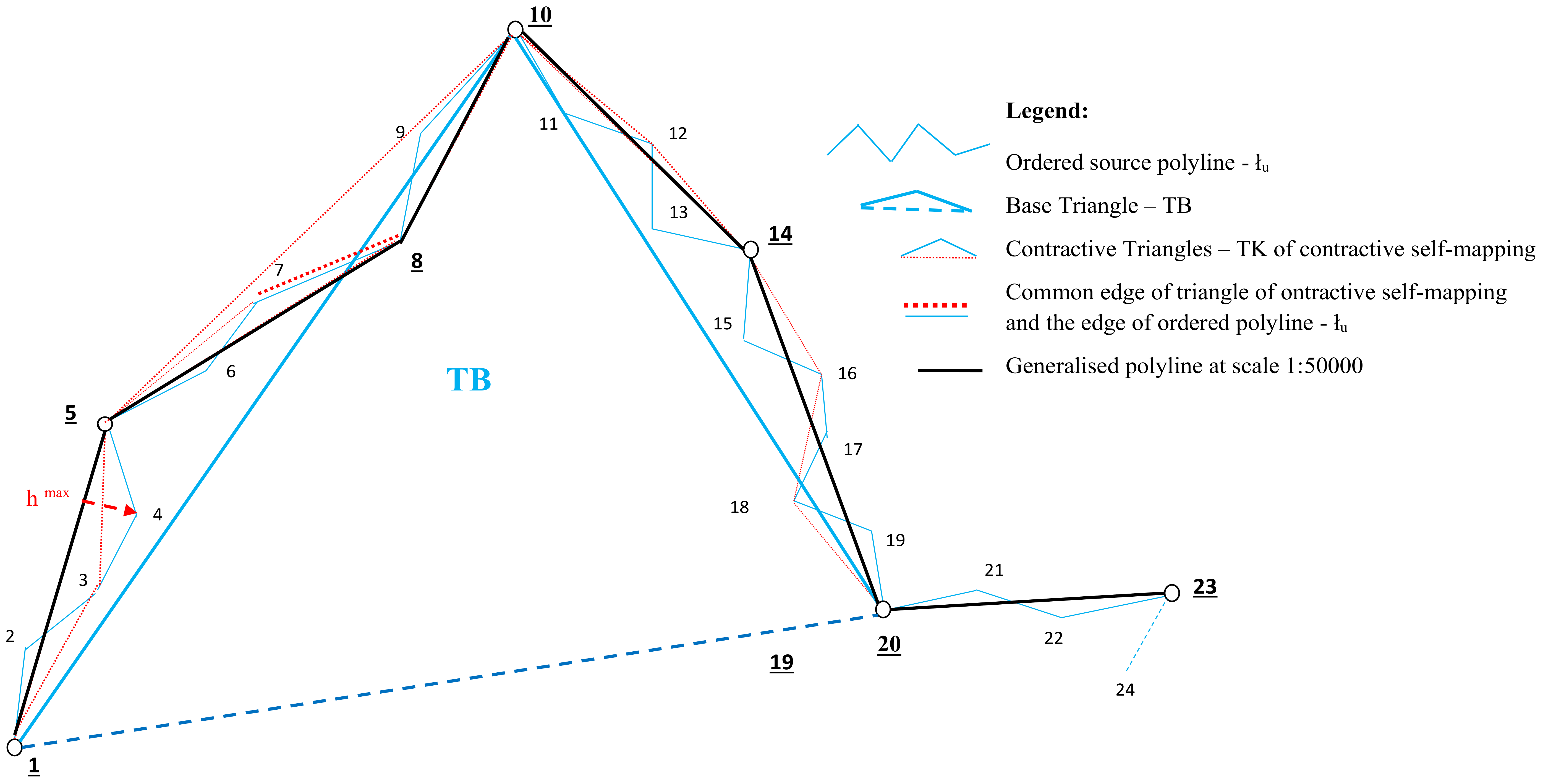
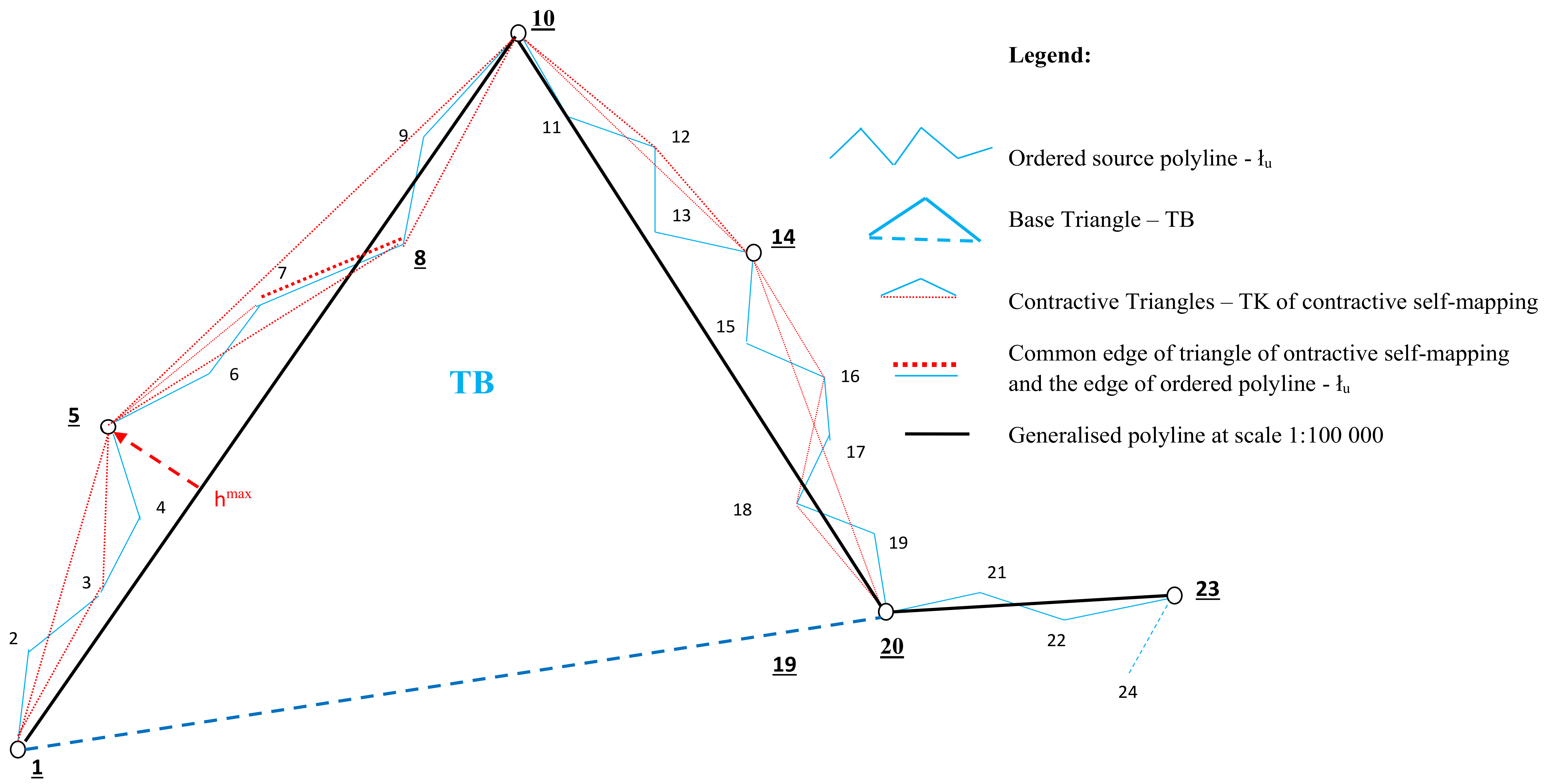
6. The Application of the Contractive Self-Mapping of Polyline ${ł}_u$ for Digital Generalisation at Scales s < 1

In contractive self-mapping, ordered polyline ${ł}_u$ belongs to metric space $L_z$. The polyline is transformed into contractive triangles TK with the application of the binary tree system, the Lipschitz condition, and the “p” bases of TK triangles in the top–down approach. Additionally, the heights h^max of the triangles TK fulfil the p > h condition in accordance with condition (2). The created triangles TK of the contractive self-mapping also fulfil the recognition norm of the minimum dimensions of triangles, as defined by, for example, A. Salishchev. If its recognition is set as a norm, the unequivocal removal of edges from the self-mapping triangles not meeting the set norm is made possible (Figure A4, Figure A5, Figure A6 and Figure A7). The remaining triangle edges form (in envelopes) the sequences of sections of the generalised line that belong to the metric space. The properties of the metric space of the generalised polyline also allow for the summation of the segments created in the envelopes. The sum of this is the objective and only result of the generalised polyline (Figure A4, Figure A5, Figure A6 and Figure A7). Then, in the created envelope, there occurs an examination of the control of the points removed from the generalised section of the segment. In the examination, this segment forms the x axis of the coordinate system, while the y axis consists of the ordinates of the points removed from the x axis. In the examined sequence of the envelope, the maximum y coordinate point (Figure A4, Figure A5, Figure A6 and Figure A7) is the height of the triangle, with the height evaluating the result in the examined envelope in accordance with the recognition norm. The results received from the envelopes that do not meet the recognition norm, end the generalisation of the polyline ${ł}_u$ at the s < 1 scale.

There are cases that exist where the generalisation of the polyline of triangle TK does not meet the norm on one edge. In such a case, the solution is to reject the second edge, and the result is the base of the triangle meeting the norm (Figure A6).

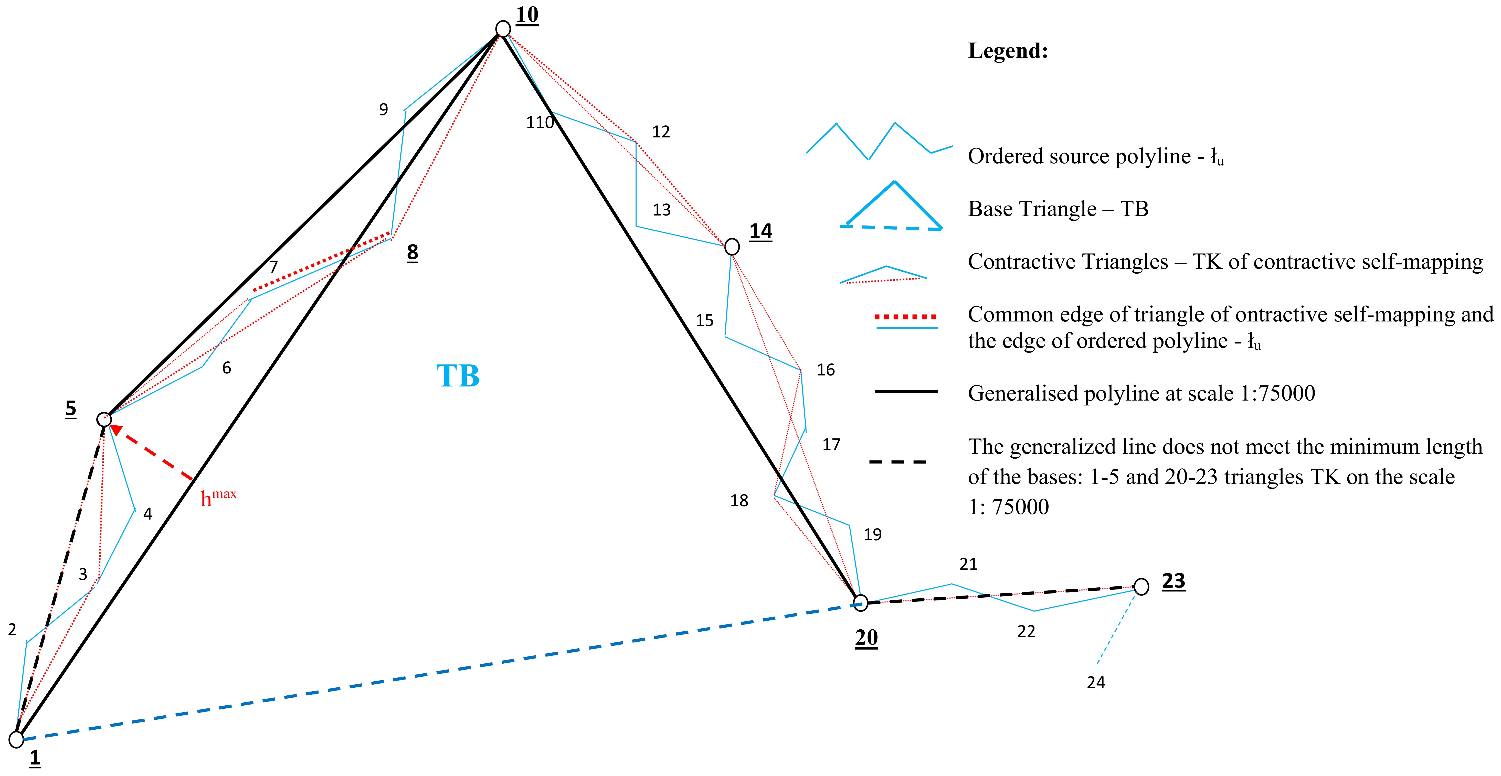
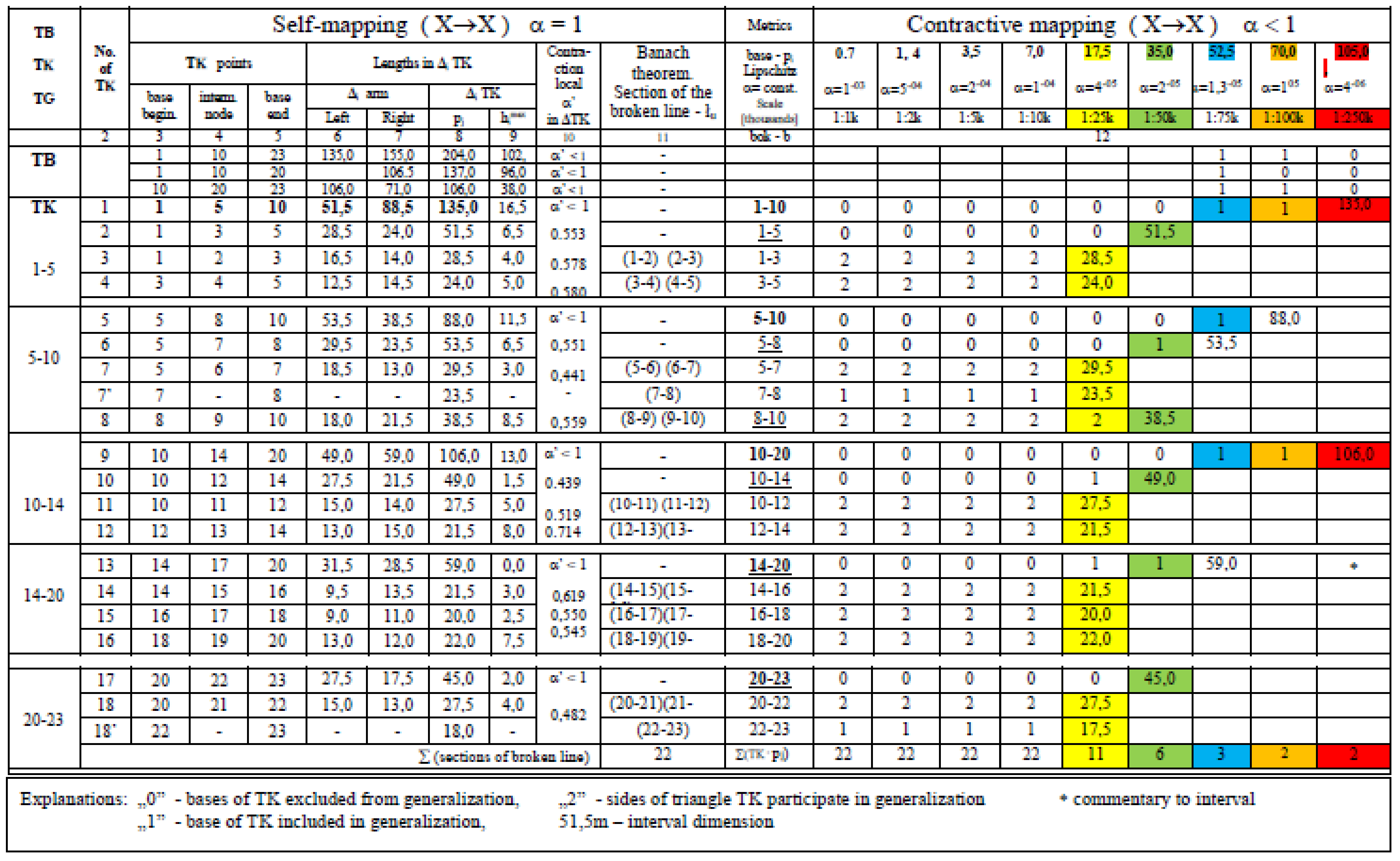
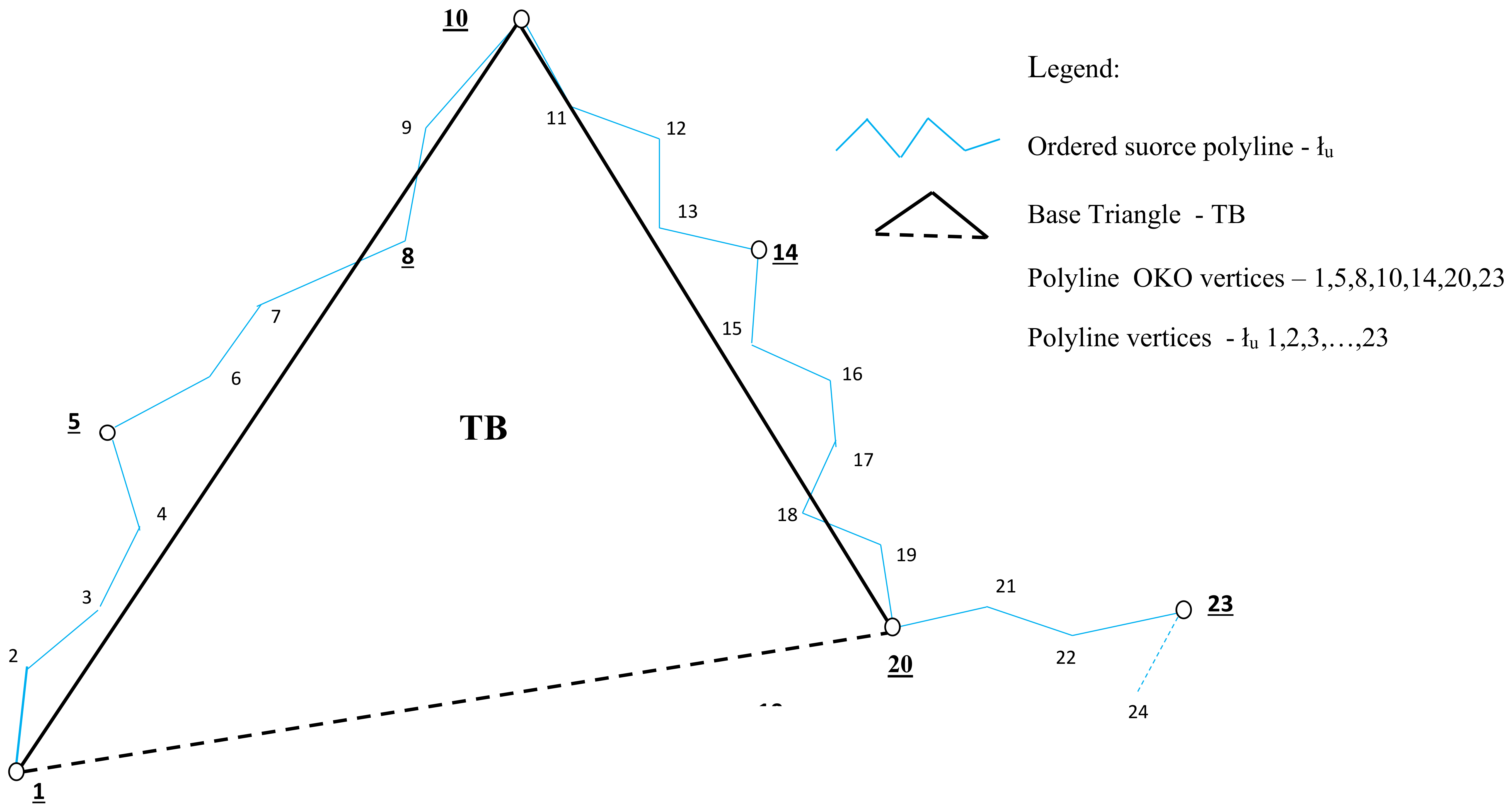
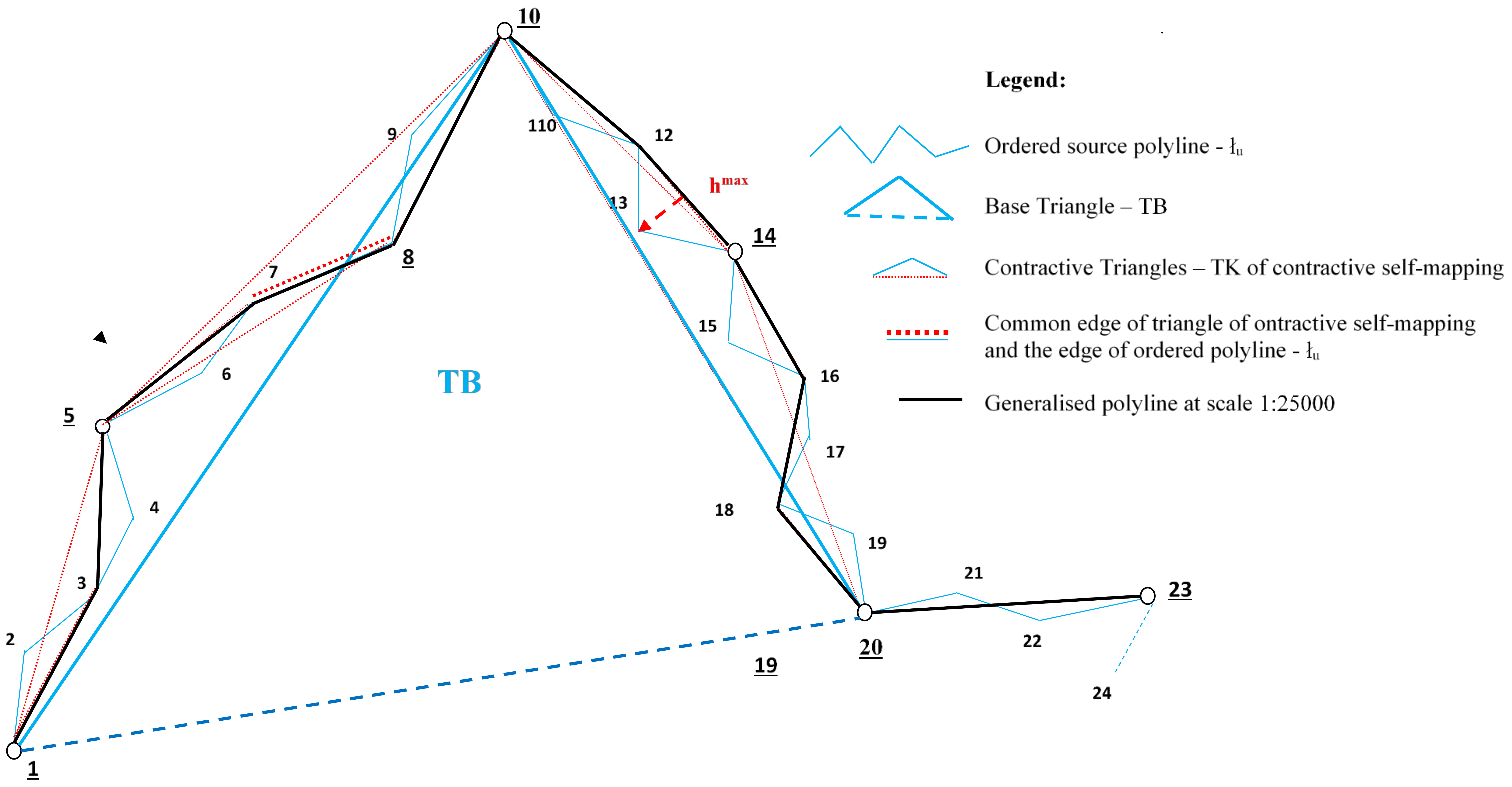
7. The Application of the Contractive Self-Mapping in Digital Generalisation at Scales s < 1, Exemplified by the Geometry of A Vistula River Fragment

The examination of the viability of contractive mapping for the objective digital generalisation of linear objects was conducted using data obtained from the Centre of Geodetic and Cartographic Documentation (NMA in Poland). The order of the data for the examination and the automation of the process has been separated into algorithms for:

(A₀) Contractive self-mapping (s = 1) of polyline ${ł}_u$,

• Input data (Figure A8):

  (a)

  Loading of vertices of line ${ł}_u$ (col. 3–5);

  (b)

  Entering the thickness of line ${ł}_u$ at scale s (col. 12);

  (c)

  Examining the recognisability of line ${ł}_u$ in accordance with the A. Salishchev metric (col. 8–9);

  (d)

  Determining the upper vertices of line ${ł}_u$, which are the polyline’s singular points (col. 3–5).

• Creation of the base triangles TB (the so-called envelopes) on line ${ł}_u$ (Figure A8):

  (a)

  Loading of singular points, which form boundaries on line ${ł}_u$ (and which double as bases of triangles TB);

  (b)

  Determination of the length of “p” chords of triangles TB from the beginning and end points of their bases (col.11);

  (c)

  Determination of the centres of the bases of TB triangles (col.11);

  (d)

  Determination of the upper vertices of TB triangles, determined from the source points of line ł (as a y intercept of the centre of the base TB with a side of line ł, and its moving to a closer point on polyline ${ł}_u$) (col.10).

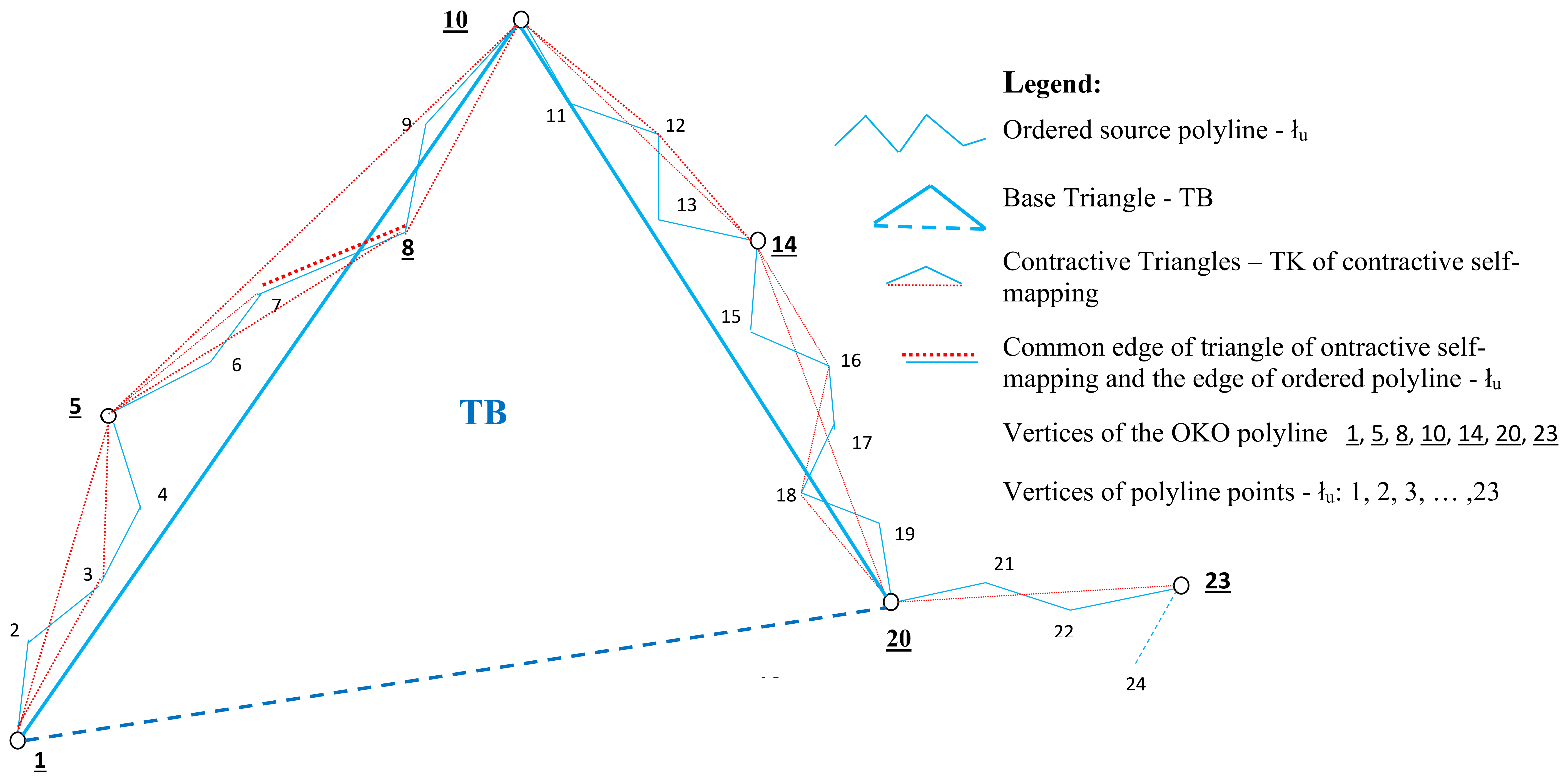
• Creation of triangles TK in envelopes of line ${ł}_u$ in accordance with the binary tree scheme (Figure A8.)

  (a)

  Determination of the left and the right side of the base triangle TB (col.6–7);

  (a)

  Determination of the vertex for the left and the right edge in triangle TB, in the same manner as described in point II.4. This results in the first triangles TK₁^L and TK₁^P of the envelope (col.10);

  (b)

  Determination of the consecutive iterations of triangles TK^L_i+1, TK^P_i+1 from the edges of the triangles from the previous iteration step, in the same manner as described in point III.2, and in accordance with the binary tree scheme (col 10);

  (c)

  Creation/formation of triangles TK on the edges of triangles TB_i^P, TB_i^L in each envelope with the top–down approach and in accordance with the binary tree scheme (col 10);

  (d)

  Contractive self-mapping ends the process in the segment of the section if the lengths of the edges of either the TKLk or TKPk triangles are the lengths of a segment of the polyline ${ł}_u$ (col.12).

• Verification of the contractive self-mapping of line ${ł}_u$:

  (a)

  In the envelope of each line ł, point III.5 is fulfilled.

(A₁) Mapping of generalisations of line ${ł}_u$ at the scale s < 1 with the use of contractive self-mapping (Figure A4.).

• Algorithm A₀ yields copies of:

  (a)

  Input data,

  (b)

  Triangles TB of base polylines ł, called envelopes, and

  (c)

  Triangles TK in the envelopes of line ł, created in accordance with the binary tree scheme.

• Creation of generalised triangles TK, depending on the scale s < 1 (Figure A8)

  (a)

  In each envelope of the polyline ł, creating the generalised polyline has an inverse relation to contracted self-mapping (i.e., bottom-up) (col.11–12);

  (b)

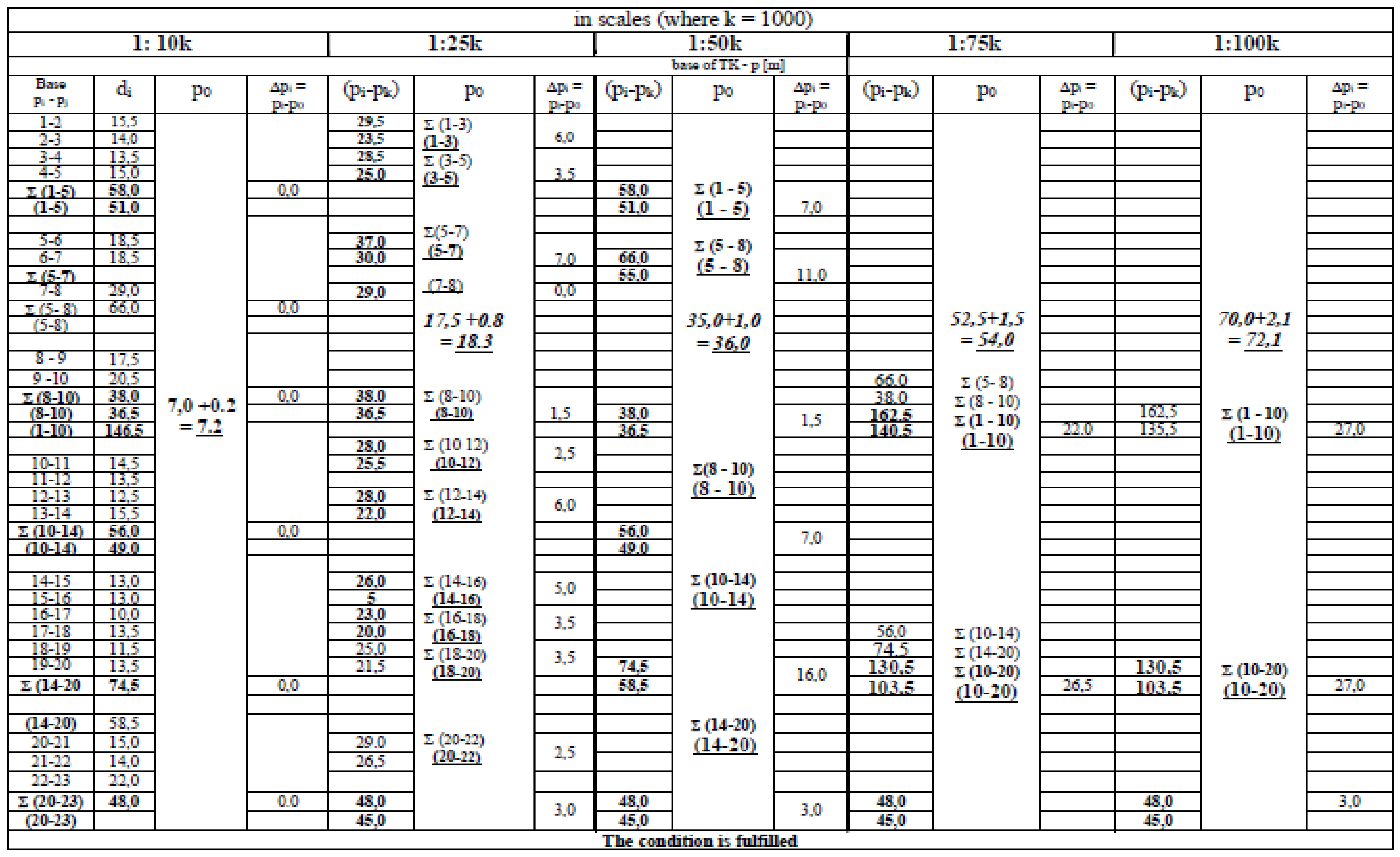
  Comparison of the dimensions of bases and the height of triangles TK with the A. Salishchev norm (col. 8–9);

  • Preservation of triangles TK meeting the A. Salishchev norm (col.12);
  • The base of triangles TK remains while their edges are discarded if their dimensions do not meet the A. Salishchev norm (Figure A5 and Figure A6);

• Creating the generalised polyline ł from the remaining points, with an unchanged order of markings of the source line (Figure A5 and Figure A6).

(A₂) Verification of generalised line ${ł}_u$ of the mapping at the scale s < 1.

• Control of the results of the generalisation of line ${ł}_u$ at scale s (Figure A9):

  (a)

  Measurement of the rejected h points of the source line ${ł}_u$ in the y coordinate envelopes against the generalised line and its created segments p of the generalised line (Figure A5, Figure A6 and Figure A7).

  (b)

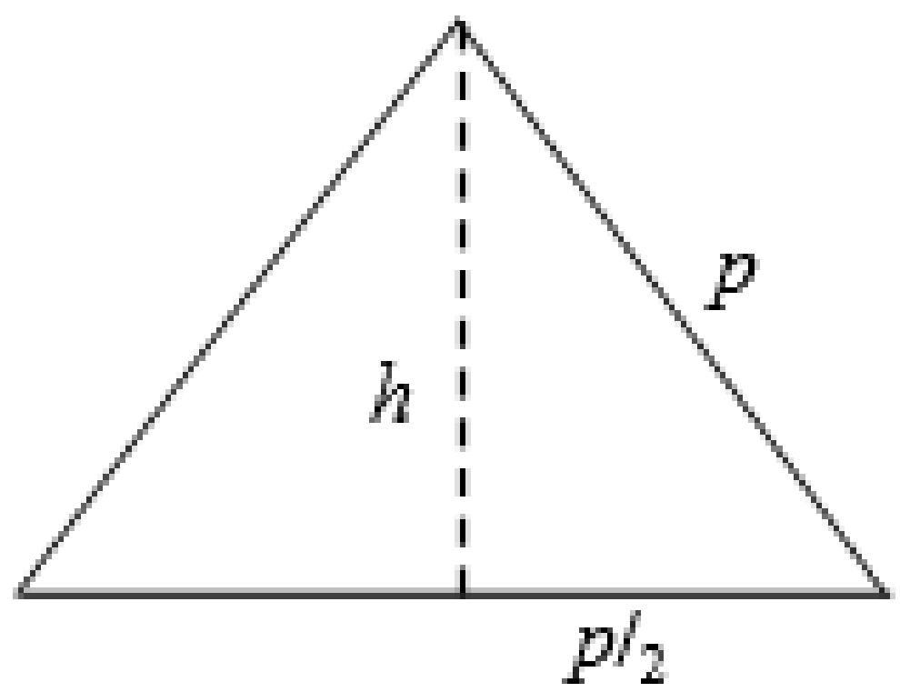
  Verification of dimensions of the Salishchev triangle at scale s through comparison (Figure A5, Figure A6 and Figure A7) of the generalised maximum height of the y coordinate h from the points of the source line ${ł}_u$ to the generalised line with a height dimension, as well as the segments p created for the generalised line with the norm of the dimensions of the base.

  (c)

  Fulfilment of the Cauchy condition from point 2 (Figure A4) and of the lengths of dimensions of the bases and the height, in accordance with the Salishchev for the generalised line ł, ends the process of Figure A5, Figure A6 and Figure A7.

The positive results of the test examinations showcased in (Figure A5, Figure A6 and Figure A7) and their verification in Figure A4 and Figure A5 allowed for the beginning of the development of the objective automated digital generalisation algorithm which is in progress.

8. Conclusions

The results of the test examinations on digital objective generalisation of object geometry allow for the following conclusions:

Each linear object in metric space in contractive self-mapping based on the binary tree structure, with the Lipschitz condition and the Banach theorem on self-contracting triangles being fulfilled has a single objective solution, which is its source data. In metric space, the multiplication operation does not change the properties of self-mapping. When adding a fixed scale s < 1 to the self-mapping and by multiplying the dimensions of the sides of the created contractive triangles by the constant “s”, we get the lengths of triangle sides for a given simplification scale. The verification of the gained data at scale “s” occurs through satisfying the Lipschitz condition and the Cauchy condition with the minimum dimensions of Salishchev, and then eliminating the sides of any contractive triangles which do not satisfy both conditions. The following conclusions are the result of their detailed study:

• Mapping, which constructs iterative images of polyline ${ł}_u$ in the form of triangles TK according to the structure of a binary tree is a contraction (Figure A5, Figure A6 and Figure A7);
• In every contraction iteration, the nodes of the polyline remaining before and after contractive self-mapping $f:X\to X$ into contractive triangles are invariant and identical (columns 3, 4, 5 with column 11 in Figure A4). This proves that triplet (${ł}_u$, $f$, $TK$) is the only one contractive mapping of an ordered polyline into itself;
• In a metric space, the contractive self-mapping f: X → X is continuous, as it fulfils the Lipschitz condition. The equation ${ł}_u=f({ł}_u)$ has one solution that results from the Banach fixed-point theorem. In addition, the sequence ${ł}_u$, $f({ł}_u)$, $f(f(({ł}_u))$, $f(f(f((({ł}_u)))$ is convergent at the “fixed point”—the polyline ${ł}_u$;.
• The ordered polyline with a binary tree structure belonging to the metric space is a constant contractive self-mapping into the contractive triangles TK of the digital generalisation at each scale s < 1, if the Lipschitz and Cauchy conditions, and the Salishchev dimensions are fulfilled. Figure A8;
• In metric space, the contractive mapping leading to generalisations of the polyline ${ł}_u$ follows the top–down approach;
• In metric space L₂, the contractive self-mapping of the polyline ${ł}_u$ is verified via its data (Figure A9). The positive result of the verification allows for the application of the contractive mapping of the polyline at scales s < 1. (Figure A8, col 12);
• The generalised polyline is unequivocally mapped if it fulfils the following conditions:

  (a)

  Source data of the polyline ${ł}_u$ belong to the metric space $L_z$, i.e., ${ł}_u\subset L_z$

  (b)

  Data of the polyline ${ł}_u$ have the binary tree structure in the mapping;

  (c)

  Transformation f of polyline ${ł}_u$ into triangles TK in its envelopes fulfils the following conditions:

  • The contractive self-mapping (data after mapping an object are source data) and at each scale s ≤ 1 fulfil: The Lipschitz contraction condition, and The assumptions of the Banach theorem;
  • at scales s < 1 (Every contraction is uniformly continuous in metric space X, as it fulfils the Lipschitz condition. The continuity of a function results from its uniform continuity.), also: the Cauchy condition with minimum dimensions of Salishchev—compatibility of summation of the after-the-mapping and removed vertices of the polyline with the number of the vertices of the source polyline ${ł}_u$;

• The method for the object geometry generalisation using the contractive self-mapping is an objective digital generalisation and has economic rationale, as:

  (a)

  One-time update of the source data can be used for all scales s ≤ 1, which significantly lowers the costs of constantly updating through their automation;

  (b)

  Data of an object at scales s < 1 are generalised with the contractive mapping, which at each scale has a single solution, in turn increases the credibility of the gained information. Contractive self-mapping used for the harmonisation of databases in which changing the scale of data is a common occurrence—and contractive self-mapping should complement the metadata of every object.

• The test examinations of the ordered polyline ${ł}_u$ in the contractive self-mapping and its generalisations included in Figure A8 and Figure A9 yielded a positive result that validates the creation of an automated application for the objective digital generalisation. Work on this problem is in progress.
• The generalisation of geospatial data appears broadly representative of current research trends, where significant positive progress can be expected in the near future [28,29]. As cartographers progress, they strategically expand existing techniques, explore new computational paradigms, and broaden their field of view [30]. Formal methods of geometry generalisation and the assessment of their impact are still not widespread or used. It seems that cartographic generalisation methods should be developed, with the aim of becoming independent from the decisions of an individual operator.

Finally, it should be emphasised that the generalisation of geospatial data is a timeless research task. It has been topical ever since the year 1857, in which von Sydow defined the three reefs of cartography. One of them is the generalisation of spatial objects, which is necessary, among other things, for the realisation of the INSPIRE directive in terms of the automation of harmonisation and the interoperability of data, which require the creation of an objective method of cartographic generalisation, of which the results are independent from the operator. The search for such a method is showcased in this paper.

An objective generalisation of data at any given scale is possible thanks to the use of the following properties: metric space, the Lipschitz contractive self-mapping theory for the triangles created with the binary tree system, the Banach theory, and the Cauchy criterion. In the verification of the generalisation results for the triangles created through the mapping, the Salishchev norms for drawing recognisability were used. The test results fully confirm the premises of this paper, especially the Banach theorem on unique solutions at each generalised scale. Currently, research on the creation of a calculation algorithm for the showcased spatial data generalisation method is in progress.

References

1. Chrobak, T. Badanie przydatności trójkąta elementarnego w komputerowej generalizacji kartograficznej [An Iinvestigation of Elementary Triangle Usefulness for Computer Cartogaphic Generalisation]; Habilitation’s Thesis, 84 Dissertations Monogarphies; UWND AGH: Kraków, Poland, 1999. [Google Scholar]
2. Mackaness, W.A.; Ruas, A. Evaluation in the Map Generalisation Process. In Generalisation of Geographic Information: Cartographic Modelling and Applications; Mackaness, W.A., Ruas, A., Sarjakoski, T.L., Eds.; Elsevier: Amsterdam, The Netherlands, 2007; pp. 89–111. [Google Scholar]
3. Douglas, D.H.; Peucker, T.K. Algorithms for the Reduction of the Number of Points Required to Represent a Digitised Line or its Caricature. Cartogr. Int. J. Geogr. Inf. Geovis. 1973, 10, 112–122. [Google Scholar] [CrossRef] [Green Version]
4. Bard, S.; Ruas, A. Why and How Evaluating Generalised Data? In Developments in Spatial Data Handling; Fisher, P.F., Ed.; Springer: Berlin/Heidelberg, Germany, 2005; pp. 327–342. [Google Scholar]
5. McMaster, R.B. A Statistical Analysis of Mathematical Measures for Linear Simplification. Cartogr. Geogr. Inf. Sci. 1986, 13, 103–116. [Google Scholar] [CrossRef]
6. Raposo, P. Scale-specific automated line simplification by vertex clustering on a hexagonal tessellation. Cartogr. Geogr. Inf. Sci. 2013, 40, 427–443. [Google Scholar] [CrossRef]
7. Töpfer, F.; Pillewizer, W. The principles of selection. Cartogr. J. 1966, 3, 10–16. [Google Scholar] [CrossRef]
8. Chrobak, T.; Szombara, S.; Kozoł, K.; Lupa, M. A method for assessing generalised data accuracy with linear object resolution verification. Geocarto Int. 2017, 32, 238–256. [Google Scholar] [CrossRef]
9. Chrobak, T.; Lupa, M.; Szombara, S.; Dejniak, D. The use of cartographic control points in the harmonization and revision of MRDBs. Geocarto Int. 2019, 34, 260–275. [Google Scholar] [CrossRef]
10. Lupa, M.; Szombara, S.; Chuchro, M.; Chrobak, T. Limits of colour perception in the context of minimum dimensions in digital cartography. ISPRS Int. J. Geo Inf. 2017, 6, 276. [Google Scholar] [CrossRef]
11. Chrobak, T. The role of least image dimensions in generalised of object in spatial databases. Geod. Cartogr. 2010, 59, 99–120. [Google Scholar]
12. Chrobak, T.; Keller, S.F.; Kozioł, K.; Szostak, M.; Żukowska, M. Podstawy Cyfrowej Generalizacji Kartograficznej. [The Basics of Digital Cartographic Generalisation]; Uczelniane Wydawnictwa Naukowo-Dydaktyczne AGH: Kraków, Poland, 2007; wyd. 1. [Google Scholar]
13. Głażewski, A.; Kowalski, P.J.; Olszewski, R.; Bac-Bronowicz, J. New Approach to Multi Scale Cartographic Modelling of Reference and Thematic Databases in Poland. In Lecture Notes in Geoinformation and Cartography, Cartography in Central and Eastern Europe Selected Papers of the 1st ICA Symposium on Cartography for Central and Eastern Europe; Gartner, G., Ortag, F., Eds.; Springer: Berlin/Heidelberg, Germany, 2010. [Google Scholar]
14. Kowalski, P.J.; Olszewski, R.; Bac-Bronowicz, J. A Multiresolution, Reference and Thematic Database as the NSDI Component in Poland—The Concept and Management Systems. In Lecture Notes in Geoinformation and Cartography, Cartography in Central and Eastern Europe Selected Papers of the 1st ICA Symposium on Cartography for Central and Eastern Europe; Gartner, G., Ortag, F., Eds.; Springer: Berlin/Heidelberg, Germany, 2010. [Google Scholar]
15. Kozioł, K.; Szombara, S. New method of creation data for natural objects in MRDB based on new simplification algorithm. In Proceedings of the 26th International Cartographic Conference; International Cartographic Association: Drezno, Germany, 2013. [Google Scholar]
16. Li, Z. Algorithmic Foundation of Multi-Scale Spatial Representation; CRC Press: London, UK, 2007. [Google Scholar]
17. Visvalingam, M.; Whyatt, J.D. Line generalisation by repeated elimination of points. Cartogr. J. 1993, 30, 46–51. [Google Scholar] [CrossRef]
18. Weibel, R. Generalisation of Spatial Data: Principles and Selected Algorithms. In Algorithmic Foundations of Geographic Information Systems; Van Kreveld, M., Nievergelt, J., Roos, T., Widmayer, P., Eds.; Springer: Berlin/Heidelberg, Germany, 1997; pp. 99–152. [Google Scholar]
19. Weibel, R. Amplified intelligence and rule-base systems. In Map Generalisation: Making Rules for Knowldege Representation; Buttenfield, B., McMaster, R., Eds.; Lonman: London, UK, 1991; pp. 172–186. [Google Scholar]
20. Blum-Krzywicka, E. Elements of Maps Contents with (0D) Point Reference Units. In Map Functions; Springer Geography Switzerland: Cham, Switzerland, 2017; pp. 41–84. [Google Scholar]
21. Burghardt, D.; Duchêne, C.; Machaness, W. Abstracting Geographic Information in a Data Rich World; Springer LNG&C: Cham, Switzerland, 2014; pp. 197–225. [Google Scholar]
22. Longley, P.A.; Goodchild, M.; Maguire, D.J.; Rhind, D.W. Geographic Information Systems and Science; Wiley: Hoboken, NJ, USA, 2010; wyd. 3. [Google Scholar]
23. Ratajski, L. Metodyka Kartografii Społeczno-gospodarczej [Methodology of the Socio-Economic Cartography]; Państwowe Przedsiębiorstwo Wydawnictw Kartograficznych im. Eugeniusza Romera: Warszawa/Wrocław, Poland, 1989; wyd. 2. [Google Scholar]
24. Directive 2007/2/ EC of the European Parliament and of the Council of 14 March 2007, known as the INSPIRE Directive. Directive 2007/2/EC of the European Parliament and of the Council of 14 March 2007 Establishing an Infrastructure for Spatial Information in the European Community (INSPIRE) | INSPIRE (europa.eu). Available online: https://inspire.ec.europa.eu/documents/directive-20072ec-european-parliament-and-council-14-march-2007-establishing (accessed on 23 February 2021).
25. Maurin, K. Analiza. Część 1 Elementy; Wydawnictwa Naukowe PWN: Warszawa, Poland, 1991; wyd. V. [Google Scholar]
26. Salishchev, K.A. Kartografia Ogólna. [General Cartography]; Wydawnictwo Naukowe PWN: Warszawa, Poland, 2003; wyd. 3. [Google Scholar]
27. Dziubiński, I.; Świątkowski, T. Poradnik Matematyczny; Warszawa PWN: Warszawa, Poland, 1982; wyd. III. [Google Scholar]
28. Liu, Y.; Li, W. A New Algorithms of Stroke Generation Considering Geometric and Structural Properties of Road Network. ISPRS Int. J. Geo Inf. 2019, 8, 304. [Google Scholar] [CrossRef] [Green Version]
29. Courtial, A.; El Ayedi, A.; Touya, G.; Zhang, X. Exploring the Potential of Deep Learning Segmentation for Mountain Roads Generalisation. ISPRS Int. J. Geo Inf. 2020, 9, 338. [Google Scholar] [CrossRef]
30. Kronenfeld, B.; Buttenfield, B.; Stanislawski, L. Map generalisation for the Future. ISPRS Int. J. Geo Inf. 2020, 9, 468. [Google Scholar] [CrossRef]
Figure 1. Cartographic control points of an aerial object.
Ijgi 10 00107 g001
Figure 2. In the TB envelope of the creation of contraction triangles TK in accordance with the binary tree system.
Ijgi 10 00107 g002
Figure 3. Determination of singular vertex.
Ijgi 10 00107 g003
Figure 4. Triangle with vertex B in a node which is a singular point.
Ijgi 10 00107 g004
Figure 5. Relation of two neighbouring triangles TK1 and TK2.
Ijgi 10 00107 g005
Figure 6. Equilateral triangle.
Ijgi 10 00107 g006
Figure 7. Operation of contractive self-mapping of a polyline into triangles TK.
Ijgi 10 00107 g007