
3D Change Detection Using Adaptive Thresholds Based on Local Point Cloud Density


1
Key Laboratory for Digital Land and Resources of Jiangxi Province, East China University of Technology, Nanchang 330013, China
2
Faculty of Geomatics, East China University of Technology, Nanchang 330013, China
3
Key Laboratory of Virtual Geographic Environment, Nanjing Normal University, Nanjing 210023, China
*
Author to whom correspondence should be addressed.
ISPRS Int. J. Geo-Inf. 2021, 10(3), 127; https://0-doi-org.brum.beds.ac.uk/10.3390/ijgi10030127
Submission received: 5 January 2021
/
Revised: 12 February 2021
/
Accepted: 19 February 2021
/
Published: 2 March 2021
(This article belongs to the Special Issue Advanced Research Based on Multi-Dimensional Point Cloud Analysis)
Abstract
:In recent years, because of highly developed LiDAR (Light Detection and Ranging) technologies, there has been increasing demand for 3D change detection in urban monitoring, urban model updating, and disaster assessment. In order to improve the effectiveness of 3D change detection based on point clouds, an approach for 3D change detection using point-based comparison is presented in this paper. To avoid density variation in point clouds, adaptive thresholds are calculated through the k-neighboring average distance and the local point cloud density. A series of experiments for quantitative evaluation is performed. In the experiments, the influencing factors including threshold, registration error, and neighboring number of 3D change detection are discussed and analyzed. The results of the experiments demonstrate that the approach using adaptive thresholds based on local point cloud density are effective and suitable.
1. Introduction
Change detection is a major topic of research in remote sensing, which plays an essential role in various tasks such as urban planning and environmental monitoring [1,2,3,4]. Three-dimensional change detection is a relatively new topic that extends change detection on 2D data to a 3D space. The demand of 3D urban modeling and updating are greatly increasing with the development and improvement of smart cities. Three-dimensional change detection can directly reflect 3D changes of objects, which is a significant desirability advantage for urban model updating [5,6,7], building and infrastructure monitoring and management [8,9,10], etc.
With the rapid development of three-dimensional laser scanning technology and the perfect progress of point cloud processing, point clouds acquired by airborne laser scanning and mobile laser scanning have been increasingly adopted in 3D change detection [11,12,13,14,15,16,17]. Moreover, point clouds can be generated through 2D data, such as UAV (Unmanned Aerial Vehicle) images [18,19,20], terrestrial images [21,22], and video sequences [23,24] in photogrammetry and computer vision. Therefore, change detection from point clouds is extremely useful in many fields. The approaches of 3D change detection based on multi-temporal point clouds can be divided to the following types, i.e., model-based comparison and point-based comparison.
(1) Model-based comparison: In order to detect changes from point clouds, this approach usually coverts point clouds to digital surface models (DSMs) and then determines changes by comparing DSMs. Murakami et al. [25] fulfilled change detection of buildings by subtracting one-point cloud-derived DSMs from another. Vogtle et al. [26] recognized building damages by comparing DSMs generated from multi-temporal airborne laser scanning data. Similar technologies have been presented in other studies, such as Chaabouni-Chouayakh et al. [27], Stal et al. [12], and Yamzaki et al. [28]. However, this method cannot detect changes in an object’s profile information since this technology mainly achieves change detection through height difference from DSMs. Some studies extracted changes by classifying DSMs derived from point clouds. Choi et al. [29] and Chaabouni-Chouayakh et al. [27] first detected change areas through the two DSMs generated from multi-temporal LiDAR data. The change areas were then classified as different objects, e.g., trees, vegetation, buildings, or grounds. Xiao et al. [30] first classified laser data-derived DSMs as different objects such as buildings and trees. The change detection was then completed based on the above classification. The accuracy of the technology depends on the object classification, which is a complex and time-consuming process.
(2) Point-based comparison: This approach directly calculates distances between points in LiDAR data. Memoli and Sapiro [31], Hyyppa et al. [5], and Antova [32] presented the point-to-point comparison framework. For each point in the detected point clouds, the distance to the nearest point in the referenced point clouds is computed. The changes are then estimated through a distance threshold. In order to improve the operating efficiency of the algorithm, Girardeau-Montaut et al. [33], Xu et al. [34], and other studies [35,36,37] performed direct comparisons with the octree structure. It is more practical for point cloud data because 3D changes can be obtained directly by point-based comparison. However, the approach is very sensitive to point cloud density. Additionally, the selection of threshold values is a key problem that influences the accuracy of change detection. Schutz and Hugli [38], and Hyyppa et al. [5] determined the changes from 3D data by a certain threshold, which was set based on empirical value. Nevertheless, some points may be skipped over or some errors may occur during distribution of the points in point clouds, which is generally nonuniform. Therefore, the certain threshold is not appropriate for change detection from the point clouds of density variation.
In this paper, adaptive thresholds based on local point cloud density are presented for point-based comparison. The k-neighboring average distance and local density in the point clouds are first calculated. The threshold values are then defined based on the k-neighboring average distance and the local point cloud density. The influencing factors including threshold, registration error, and neighboring number of 3D change detection are analyzed in the experiments.
2. Methods
In this paper, 3D change detection from point clouds is presented by point-based comparison. The k-neighboring average distance of each point in the detected point clouds and the local densities of the k-neighboring points are calculated. The distance thresholds for identifying changes are given, combined with the k-neighboring average distance and the local densities.
2.1. Preliminaries
Point-to-point comparison based on closest point distance is the simplest and fastest way to detect 3D change between two point clouds as it does not require gridding or meshing of the data or calculation of the surface normal [33]. The nearest neighboring distance is calculated as the distance between two points: for each point in the detected point clouds, the nearest point in the referenced point clouds is searched and their Euclidean distance is computed [39].
For two point clouds, PC1 and PC2 (PC1 is the detected point clouds, and PC2 is the referenced point clouds), at different periods, the nearest neighboring distance is computed between a point in PC1 and its nearest neighboring point in PC2.
The following expression can be used to determine changes between PC1 and PC2.
where is the threshold to determine whether changes occurred between PC1 and PC2. Generally, is set as a stationary value based on experience or the average distance of all the points in PC1 and PC2. However, the local density variation of the point clouds is not considered in these algorithms using a certain threshold or the average distance of all the points in the point clouds.
2.2. Adaptive Thresholds Based on Local Point Cloud Density
To take into account the local density variation of the point clouds, the threshold values are defined through the k-neighboring average distance and local point densities in the point clouds.
2.2.1. K-Neighboring Average Distance
The local average distance for the point and its k-neighboring points can be calculated as follows:
where is the nearest neighboring point of in the point clouds P.
Then, the k-neighboring average distance of all the points in P is the mean value of the local average distances .
where n is the number of points in P.
2.2.2. Local Point Cloud Density
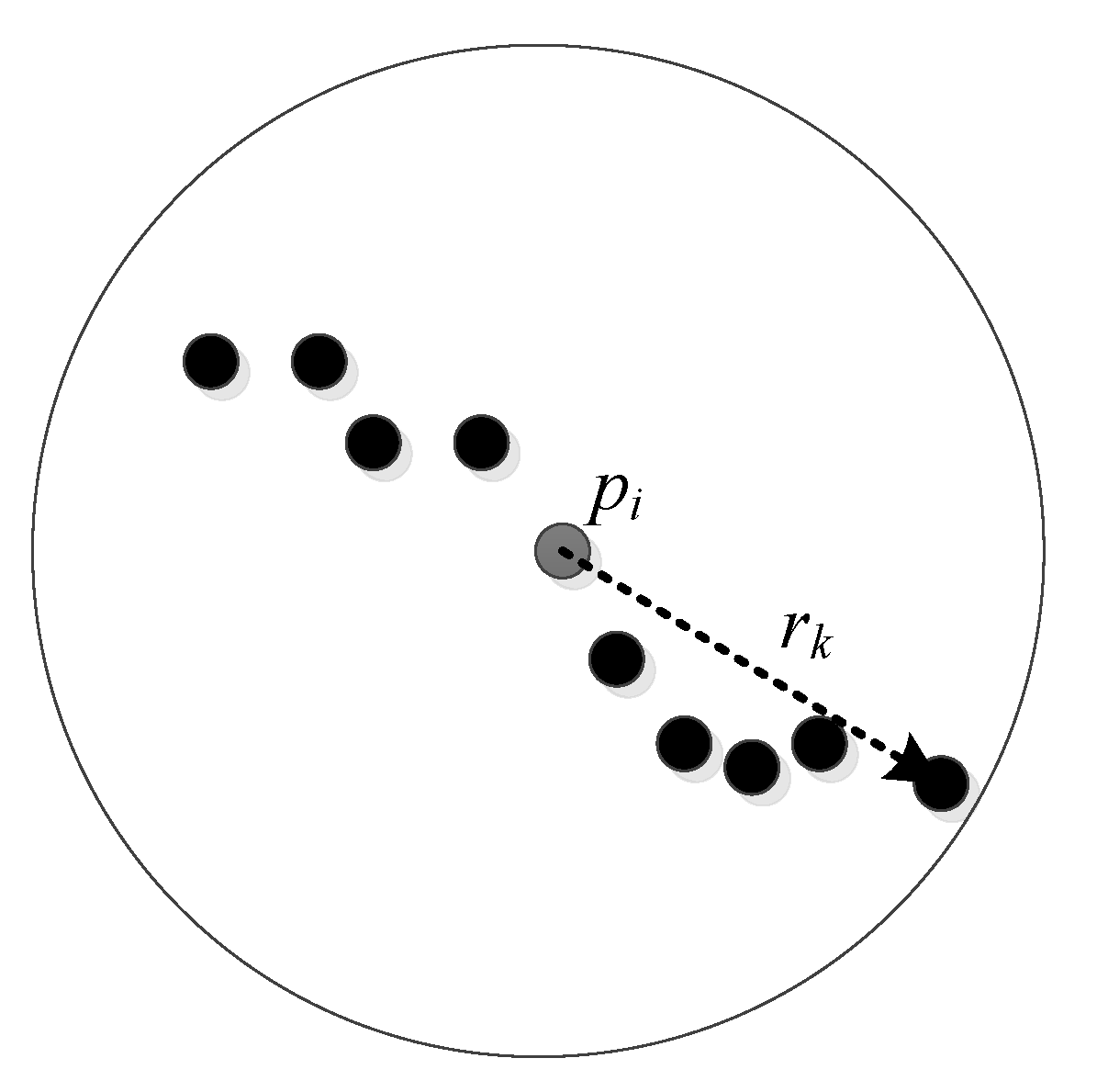
For the given point in the point clouds P, the local point cloud density index can be estimated as follows:
where k is the number of neighboring points to the point and is the area of the circle centered at the point with a radius that is the fastest distance from the point to its k-nearest neighboring points (Figure 2).
Then, the local point cloud densities of all the points in P are normalized by logarithmic function and rescaled to the range [0,1].
According to the overall characteristics of the point cloud density, a larger value means a higher density of the local points. Thus, the threshold for change detection should be less.
According to Equations (5) and (6), the thresholds can be expressed as follows:
where represents the threshold of point ; k is the number of neighboring points to point ; and is a constant coefficient, which can be set to [1,3]. In the experiments presented in this paper, it is set as .
2.3. Implementation of 3D Change Detection Using Adaptive Thresholds
For the compared point clouds PC1 and the referenced point clouds PC2, the overall algorithm of change detection for each point in the point clouds PC1 is as follows:
- (1)
- Select a point in the compared point clouds PC1.
- (2)
- In the referenced point clouds PC2, search the nearest point to the point .
- (3)
- According to Equation (1), calculate the Euclidean distance .
- (4)
- In the point clouds PC1, search the k-neighboring points to the point .
- (5)
- According to Equations (3) and (4), compute the k-neighboring average distance of PC1.
- (6)
- According to Equations (5) and (6), compute the local point density and its normalized value .
- (7)
- Calculate the threshold of point using Equation (7).
- (8)
- Detect whether point has changed. If , then a change in has occurred.
- (9)
- Use the above steps to detect changes in all the points in the point cloud PC1.
3. Experimental Results and Discussion
In order to determine the accuracy and effectiveness of the proposed approach, a series of experiments using test data was performed.
3.1. Experimental Data
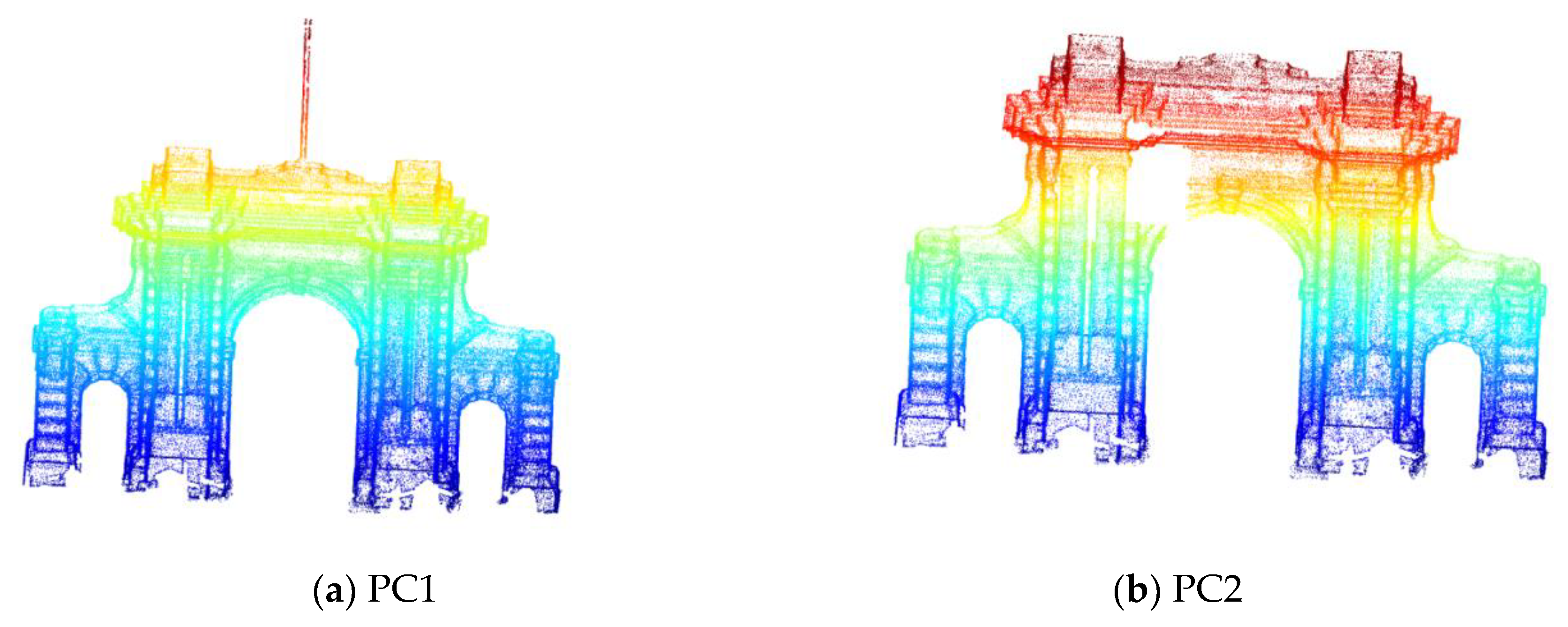
In the experiments, the test data shown in Figure 3a were captured by the terrestrial laser scanner system Riegl-LMS-Z420i with a single shot accuracy of 10 mm at 50 m [40]. The test data were the building from the old gate of Tsinghua University in the city of Beijing, China. To evaluate the performance of 3D change detection based on point clouds, the test data in Figure 3a were used as a temporal point cloud data named PC1. There were 168,603 points in the point clouds PC1. The other temporal data, PC2, shown in Figure 3b, were generated by deleting some points in PC1.
Considering the influence of the threshold and neighboring number on the results of 3D change detection, several series of experiments with the test data were performed. To quantitatively assess the accuracies of the 3D change detection results on the test data, the following four quantitative measures were used: completeness, correctness, quality, and [41]. Completeness represents the proportion of correctly detected change points to the true change points. Correctness, which is the proportion of correctly detected change points to all the detected change points, estimates the reliability of 3D change detection. Quality and indicate the overall performance of change detection. They are defined as follows:
where TP (true position) is the number of correctly detected change points, FP (false position) is the number of non-changed points incorrectly detected as changed, and FN (false negative) is the number of change points falsely detecting non-changed points.
3.2. Results and Discussion
(1) Experiment 1 (Varying the registration error)
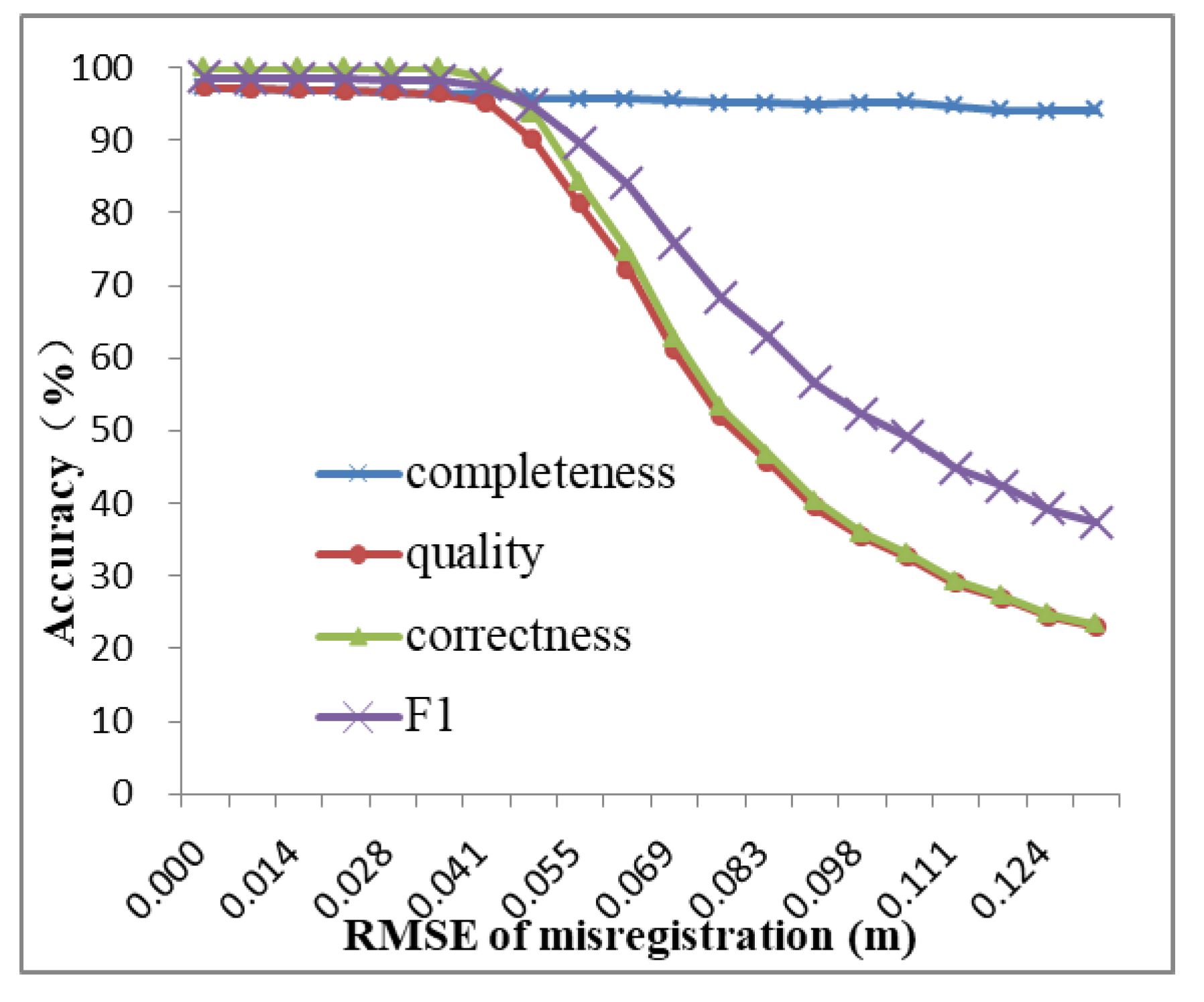
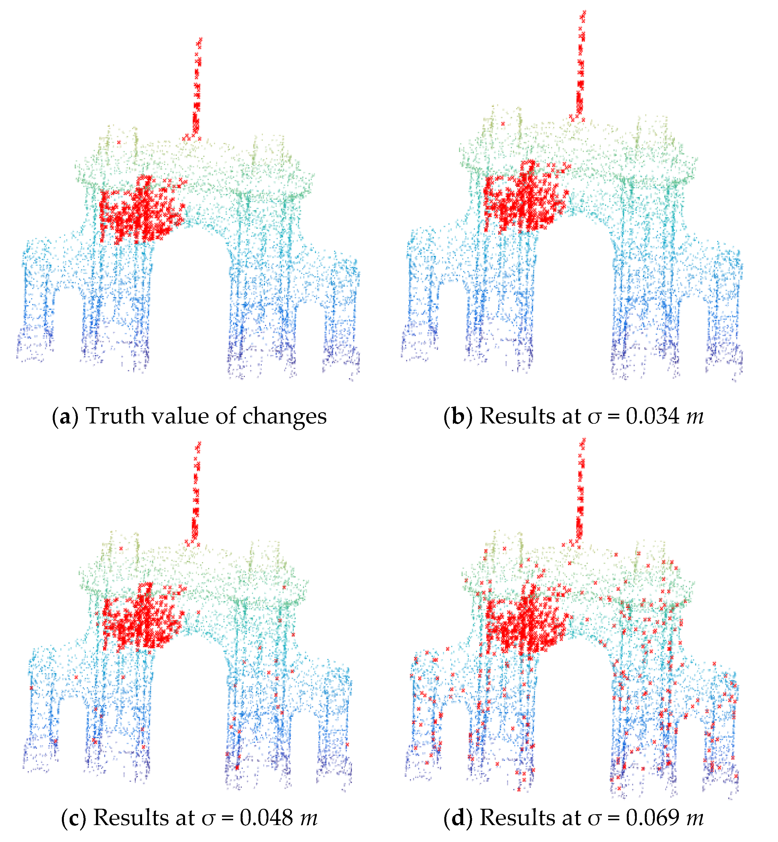
In the first series of experiments, 5% of the test data PC1 and PC2 were randomly sampled. After sampling, the average distance of PC1 was found to be 0.067 m. PC1 and PC2 were progressively misregistered by Gaussian noise with mean 0 and standard deviations 0, 0.004, 0.008, …, 0.076 m that was added to each point of PC1. It corresponds to the root mean square errors (RMSEs) 0, 0.007, 0.014, 0.021, 0.028, 0.034, 0.041, 0.048, 0.055, 0.062, 0.069, 0.076, 0.083, 0.09, 0.098, 0.104, 0.111, 0.118, 0.124, and 0.133 m in total misregistration. Three-dimensional changes using adaptive thresholds in this paper were detected based on PC1 and PC2. The number of neighboring points was set as 50, i.e., . The results are shown in Figure 4 and Table 1. The qualitative results of 3D change detection with different registration errors are presented in Figure 5a–d.
From the results illustrated in Figure 4, Figure 5, and Table 1, the following considerations can be outlined.
- (a)
- As the misregistration of two point clouds increases, the values of the indicators correctness, quality, and F1 obtained through Equation (8) become lower. There is no evident changes in the value of completeness (completeness > 90% in all the errors of image registration), which means that most of the change points can be detected correctly. However, FP, i.e., non-changed points incorrectly detected as change points, becomes larger as the registration error increases. Therefore, misregistration of point clouds has significant effects on 3D change detection.
- (b)
(2) Experiment 2 (Different threshold values T)
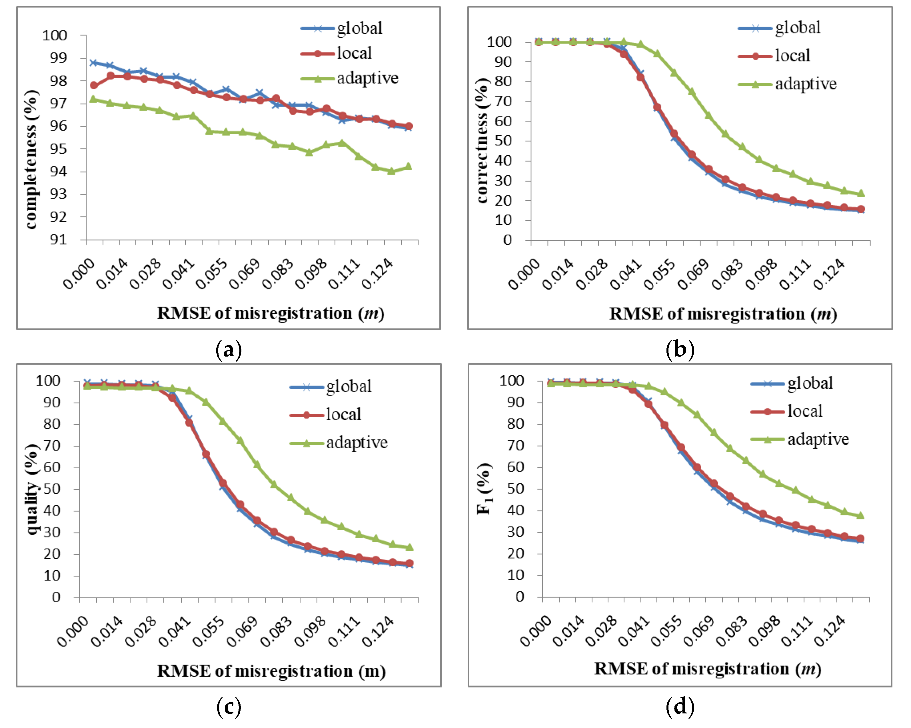
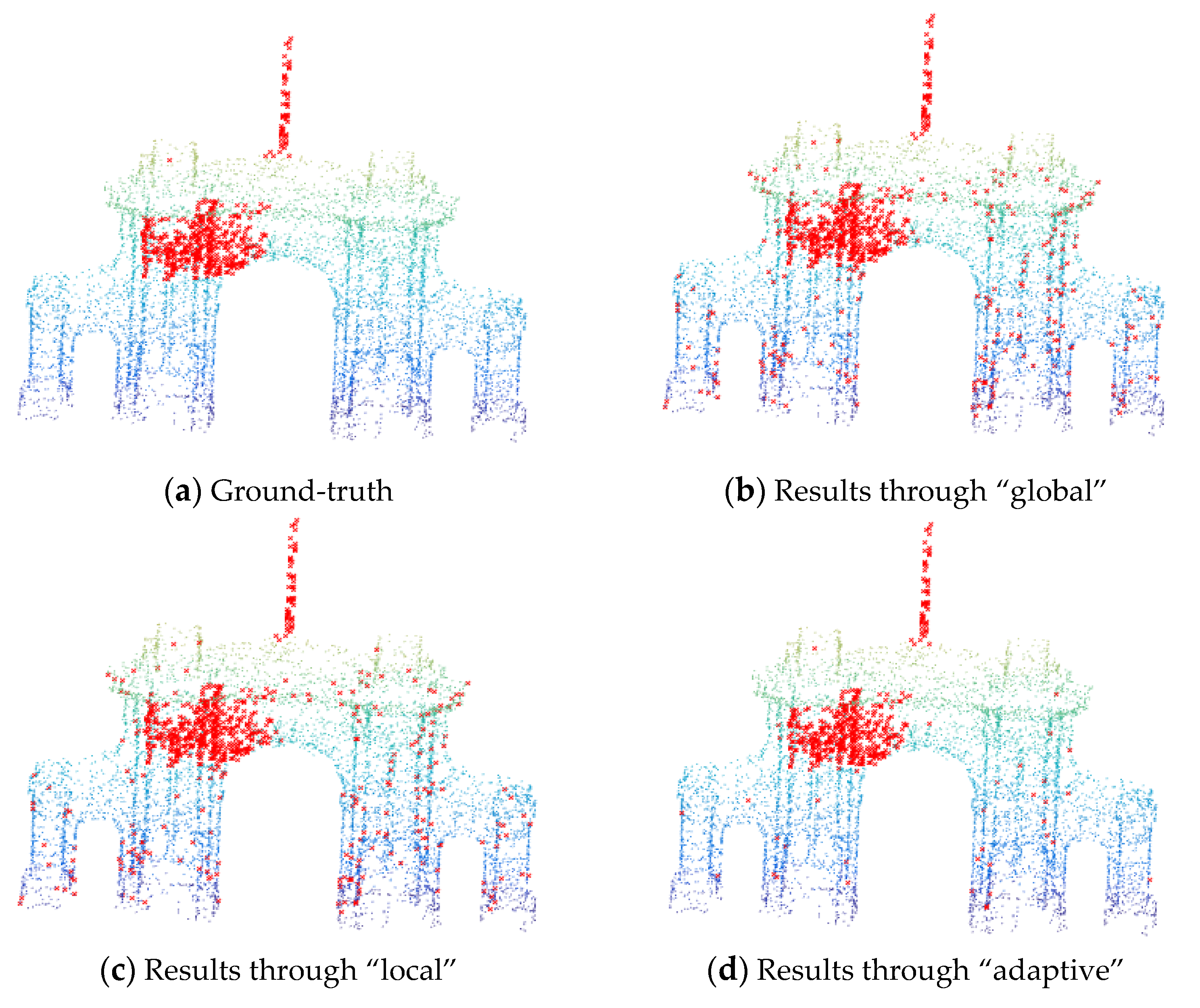
Like the first series of experiments, the processes of sampling and adding noise are done in this series experiments. To compare the results obtained using adaptive thresholds, the methods use the global average distance () and the local average distances (i.e., calculated by Equation (3)). The results based on different threshold values T are shown in Figure 6a–d and Figure 7a–d. In Figure 6 and Figure 7, “global” represents the results obtained by using the global threshold, i.e., the average distance of all the points in PC1; “local” represents the results using the local average distances as the thresholds; and “adaptive” represents the results using adaptive thresholds in this paper. The number of neighboring points is set as 50 for “local” and “adaptive”. The results presented in Figure 7b–d are obtained in the condition of misregistration 0.048 m.
From the results illustrated in Figure 6 and Figure 7, the following considerations can be remarked.
- (a)
- When the registration error is very weak, all the methods using the above three thresholds can obtain appropriate accuracy. However, the method using the adaptive thresholds significantly outperforms the other methods with the increase in registration error .
- (b)
- When the registration error is larger than 0.04 m, the performance of change detection using the global and local thresholds decline rapidly. Thus, the registration error of the point clouds should be less than 1/2 of the average distance of point clouds for 3D change detection using the global and local thresholds. However, for the method using the adaptive thresholds, the registration error can be relaxed to the average distance of the point clouds. Therefore, the method using adaptive thresholds can obtain more satisfactory results than the two other methods.
(3) Experiment 3 (Varying the number of the neighboring points k)
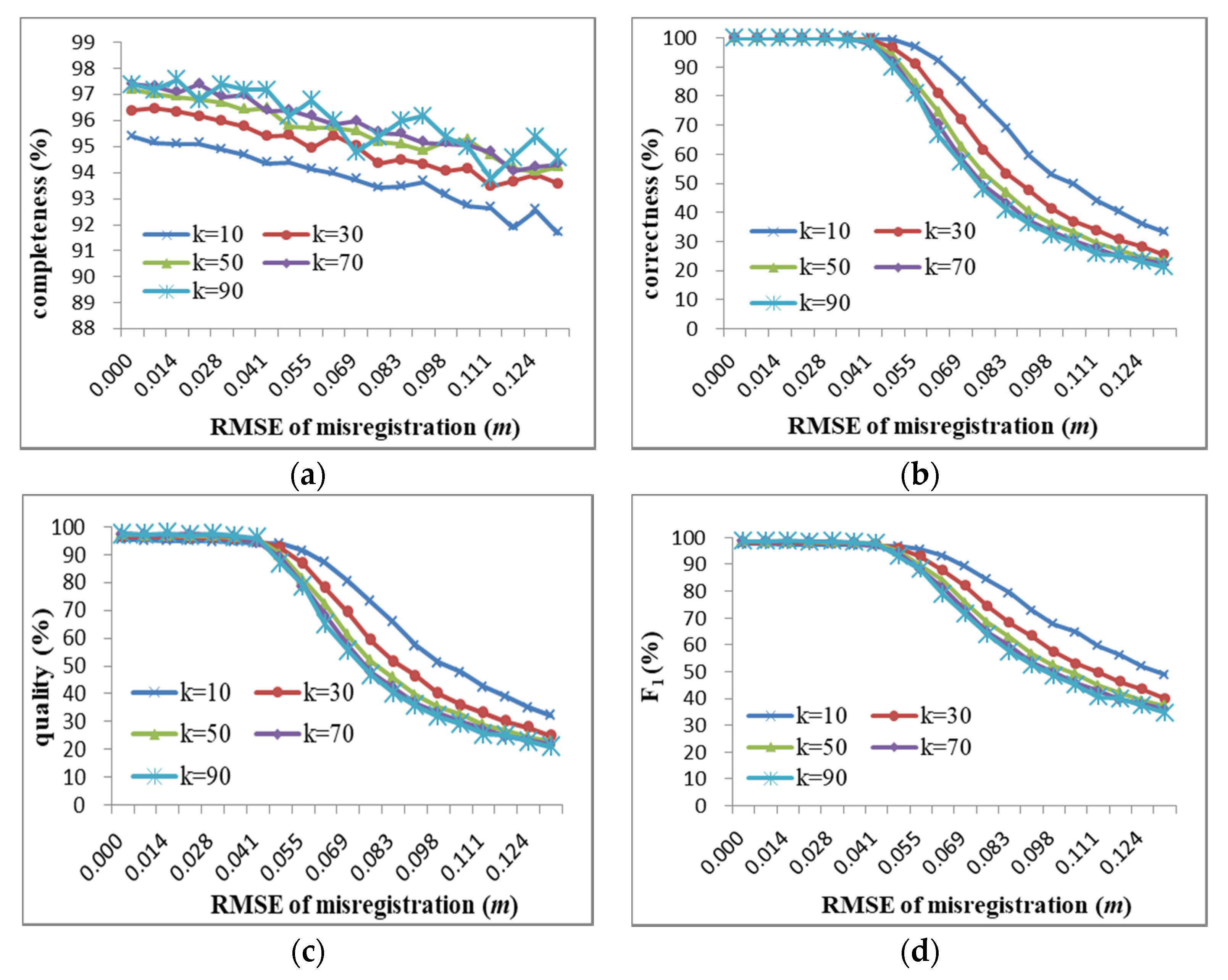
In the third series of experiments, the test data were the same as that in experiment 1 except the number of neighboring points varied. The number of neighboring points was set as 10, 30, 50, 70 and 90. The results are presented in Figure 8a–d.
As the number of neighboring points increases, the method using adaptive thresholds has higher data accuracy, with the registration error being better than 0.041 m. However, the accuracy is lower with an increasing number of neighboring points k when the registration error is over 0.041 m. Moreover, the results of 3D change detection have no evident changes at . Therefore, the setting of k can be adjusted according to the registration error. k can be set to smaller values when the registration error is less than 1/2 of the average distance of point clouds. Instead, k can be set within a larger value (such as ) when the registration error is larger than 1/2 of the average distance of point clouds.
4. Conclusions
In this paper, the development and implementation of 3D change detection based on a point-based comparison from point cloud data is presented. A particular feature of this approach is that adaptive thresholds are used to detect changes in the point clouds. To consider local density variation of the point clouds, the adaptive thresholds are calculated in combination with the k-neighboring average distance and the local point cloud density. Additionally, the influence of the registration error and the number of neighboring points on the accuracy of 3D change detection are investigated. A series of experiments on test data are presented in this paper. Compared with common methods with thresholds of global average distance and local average distance of point clouds, the experiments demonstrate that the approach based on adaptive thresholds is less affected by the registration error between point clouds. The experimental results show that the registration error for the approach using adaptive thresholds could be controlled within the average distance of the point clouds. Moreover, the number of neighboring points could select an appropriate value according to the registration error. Future work will focus on optimization of the algorithms in terms of the computation cost, etc.
Author Contributions
Dan Liu and Dajun Li conceived and designed the experiments; Dan Liu performed the experiments; Dan Liu and Meizhen Wang contributed to the analysis and interpretation of the results; Dan Liu wrote the manuscript; Dajun Li and Zhiming Wang revised the manuscript. All authors have read and agreed to the published version of the manuscript.
Funding
The work described in this paper was support by the National Natural Science Foundation of China (Project No: 41701437); by the Science and Technology Program of the Education Department of Jiangxi Province of China (Project No: GJJ180420); and by the Key Laboratory for Digital Land and Resources of Jiangxi Province, East China University of Technology (Project No: DLLJ201805).
Institutional Review Board Statement
Not applicable.
Informed Consent Statement
Not applicable.
Data Availability Statement
Publicly available datasets were analyzed in this study. This data can be found here: [http://vision.ia.ac.cn/data (accessed on 1 March 2021)].
Acknowledgments
Thank you to the China and National Laboratory of Pattern Recognition, Institute of Automation, Chinese Academy of Sciences, China. We also would like to express our gratitude to the anonymous reviewers for their comments and suggestions to this article.
Conflicts of Interest
The authors declare no conflict of interest.
References
- Zhang, Q.; Wang, J.; Peng, X.; Gong, P.; Shi, P. Urban built-up land change detection with road density and spectral information from multi-temporal Landsat TM data. Int. J. Remote Sens. 2002, 23, 3057–3078. [Google Scholar] [CrossRef]
- Im, J.; Jensen, J.R. A change detection model based on neighboring correlation image analysis and decision tree classification. Remote Sens. Environ. 2005, 99, 326–340. [Google Scholar] [CrossRef]
- Lin, Y.; Zhang, L.; Wang, N.; Zhang, X.; Cen, Y.; Sun, X. A change detection method using spatial-temporal-spectral information from Landsat images. Int. J. Remote Sens. 2019, 41, 1–22. [Google Scholar] [CrossRef]
- Bolorinos, J.; Ajami, N.K.; Rajagopal, R. Consumption Change Detection for Urban Planning: Monitoring and Segmenting Water Customers during Drought. Water Resour. Res. 2020, 56, 1217–1248. [Google Scholar] [CrossRef]
- Hyyppa, J.; Jaakkola, A.; Hyyppa, H.; Kaartinen, H.; Kukko, A.; Holopainen, M.; Zhu, L.; Vastaranta, M.; Kaasalainen, S.; Krooks, A.; et al. Map updating and change detection using vehicle-based laser scanning. In Proceedings of the 2009 Joint Urban Remote Sensing Event, Shanghai, China, 20–22 May 2009. [Google Scholar]
- Kim, C.; Kim, B.; Kim, H. 4D CAD Model updating using image processing-based construction progress monitoring. Autom. Constr. 2013, 35, 44–52. [Google Scholar] [CrossRef]
- Matikainen, L.; Pandi, M.; Li, F.S.; Karila, K.; Hyyppä, J.; Litkey, P.; Kukko, A.; Lehtomäki, M.; Karjalaine, M.; Puttonen, E. Toward utilizing multitemporal multispectral airborne laser scanning, Sentinel-2, and mobile laser scanning in map updating. J. App. Remote Sens. 2019, 13, 044504. [Google Scholar] [CrossRef]
- Leena, M.; Juha, H.; Eero, A.; Markelin, L.; Kaartinen, H. Automatic detection of buildings and changes in buildings for updating of maps. Remote Sens. 2010, 2, 1217–1248. [Google Scholar]
- Rebolj, D.; Babi, N.U.; Magdi, A.; Podbreznik, P.; Pšunder, M. Automated construction activity monitoring system. Adv. Eng. Inform. 2008, 22, 493–503. [Google Scholar] [CrossRef]
- Li, W.; Sun, K.; Li, D.; Bai, T.; Sui, H. A New Approach to Performing Bundle Adjustment for Time Series UAV Images 3D Building Change Detection. Remote Sens. 2017, 9, 625. [Google Scholar] [CrossRef] [Green Version]
- Chen, B.; Deng, L.; Duan, Y.; Huang, S.; Zhou, J. Building change detection based on 3D reconstruction. In Proceedings of the 2015 IEEE International Conference on Image Processing, Quebec, QC, Canada, 27–30 September 2015. [Google Scholar]
- Stal, C.; Tack, F.; Maeyer, P.D.; Wulf, A.D.; Goossens, R. Airborne photogrammetry and LiDAR for DSM extraction and 3D change detection over an urban area—A comparative study. Int. J. Remote Sens. 2013, 34, 1087–1110. [Google Scholar] [CrossRef] [Green Version]
- Kim, A.M.; Runyon, S.C.; Jalobeanu, A.; Esterline, C.H.; Kruse, F.A. LiDAR change detection using building models. In Proceedings of the SPIE 9080, Laser Radar Technology & Applications Xix & Atmospheric Propagation XI, Baltimore, MD, USA, 6–7 May 2014. [Google Scholar]
- Qin, R.; Tian, J.; Reinartz, P. 3D change detection—Approaches and applications. ISPRS J. Photogramm. Remote Sens. 2016, 122, 41–56. [Google Scholar] [CrossRef] [Green Version]
- Dong, P.L.; Zhong, R.F.; Yigit, A. Automated parcel-based building change detection using multitemporal airborne LiDAR data. Survey. Land Inform. Sci. 2018, 77, 5–13. [Google Scholar]
- Shirowzhan, S.; Samad, S.M.E.; Li, H.; Trinder, J.; Tang, P. Comparative analysis of machine learning and point-based algorithms for detecting 3D changes in buildings over time using bi-temporal LiDAR data. Autom. Construct. 2019, 105, 102841. [Google Scholar] [CrossRef]
- Santos, R.C.D.; Galo, M.; Carrilho, A.C.; Pessoa, G.G.; de Oliveira, R.A.R. Automatic building change detection using multi-temporal airbone Lidar data. In Proceedings of the International Archives of the Photogrammetry, Remote Sensing and Spatial Information Sciences, 2020 IEEE Latin American GRSS & ISPRS Remote Sensing Conference, Santiago, Chile, 21–26 March 2020; Volume XLII-3/W12-2020. [Google Scholar]
- Eltner, A.; Schneider, D. Analysis of Different Methods for 3D Reconstruction of Natural Surfaces from Parallel-Axes UAV Images. Photogramm. Rec. 2015, 30, 279–299. [Google Scholar] [CrossRef]
- Qu, Y.; Huang, J.; Zhang, X. Rapid 3D Reconstruction for Image Sequence Acquired from UAV Camera. Sensors 2018, 18, 225. [Google Scholar]
- Shahbazi, M.; Menard, P.; Sohn, G.; Théau, J. Unmanned aerial image dataset: Ready for 3D reconstruction. Data Brief 2019, 25, 103962. [Google Scholar] [CrossRef] [PubMed]
- Adilson, B.; Tommaselli, A.M.G. Automatic Orientation of Multi-Scale Terrestrial Images for 3D Reconstruction. Remote Sens. 2014, 6, 3020–3040. [Google Scholar]
- Liu, D.; Liu, X.J.; Wu, Y.G. Depth Reconstruction from Single Images Using a Convolutional Neural Network and a Condition Random Field Model. Sensors 2018, 18, 1318. [Google Scholar] [CrossRef] [PubMed] [Green Version]
- Kundu, A.; Li, Y.; Dellaert, F.; Li, F.; Rehg, J.M. Joint Semantic Segmentation and 3D Reconstruction from Monocular Video. In Proceedings of the European Conference on Computer Vision, Zurich, Switzerland, 6–12 September 2014; Springer: Cham, Switzerland, 2014. [Google Scholar]
- Gerdes, K.; Pedro, M.Z.; Schwarz-Schampera, U.; Schwentner, M.; Kihara, T.C. Detailed Mapping of Hydrothermal Vent Fauna: A 3D Reconstruction Approach Based on Video Imagery. Front. Marine Sci. 2019, 6, 1–21. [Google Scholar] [CrossRef] [Green Version]
- Murakami, H.; Nakagawa, K.; Hasegawa, H.; Shibata, T.; Iwanami, E. Change detection of buildings using an airborne laser scanner. ISPRS J. Photogramm. Remote Sens. 1999, 54, 148–152. [Google Scholar] [CrossRef]
- Vögtle, T.; Steinle, E. Detection and recognition of changes in building geometry derived from multitemporal laser scanning data. Int. Arch. Photogramm. Remote Sens. Spat. Inf. Sci. 2004, 428–433. [Google Scholar]
- Chaabouni-Chouayakh, H.; Krauss, T.; d’Angelo, P.; Peter, R. 3D change detection inside urban areas using different digital surface models. In Proceedings of the PCV 2010—ISPRS Technical Commission III Symposium on Photogrammetry Computer Vision and Image Analysis, Paris, France, 1–3 September 2010. [Google Scholar]
- Yamazaki, F.; Liu, W.; Moya, L. Use of multitemporal LiDAR data to extract changes due to the 2016 Kumamoto earthquake. In Proceedings of the Remote Sensing Technologies and Applications in Urban Environments II, Warsaw, Poland, 11–12 September 2017. Society of Photo-Optical Instrumentation Engineers (SPIE) Conference Series. [Google Scholar]
- Choi, K.; Lee, I.; Kim, S. A feature based approach to automatic change detection from LiDAR data in urban areas. Int. Arch. Photogramm. Remote Sens. 2009, 25, 259–264. [Google Scholar]
- Xiao, W.; Xu, S.; Elberink, S.O.; Vosselman, G. Change detection of trees in urban areas using multi-temporal airborne LiDAR point clouds. In Proceedings of the Remote Sensing of the Ocean, Sea Ice, Coastal Waters, and Large Water Regions, Edinburgh, UK, 26–27 September 2012. [Google Scholar]
- Memoli, F.; Sapiro, G. Comparing point clouds. In Proceedings of the Eurographics Symposium on Geometry Processing, Nice, France, 8–10 July 2004; pp. 32–40. [Google Scholar]
- Antova, G. Application of areal change detection methods using point clouds data. Earth Environ. Sci. 2019, 221, 012082. [Google Scholar] [CrossRef]
- Girardeau-Montaut, D.; Roux, M.; Marc, R.; Marc, R.; Thibault, G. Change detection on point cloud data acquired with a ground laser scanner. In Proceedings of the ISPRS Workshop Laser Scanning, Enschede, The Netherlands, 12–14 September 2005. [Google Scholar]
- Xu, H.; Cheng, L.; Li, M.; Chen, Y.; Zhong, L. Using Octrees to Detect Changes to Buildings and Trees in the Urban Environment from Airborne LiDAR Data. Remote Sens. 2015, 7, 9682–9704. [Google Scholar] [CrossRef] [Green Version]
- Xiao, W.; Vallet, B.; Paparoditis, N. Change detection in 3D point clouds acquired by a mobile mapping system. In Proceedings of the ISPRS Annals of the Photogrammetry, Remote Sensing and Spatial Information Sciences, Antalya, Turkey, 11–13 November 2013. [Google Scholar]
- Hebel, M.; Arens, M.; Stilla, U. Change detection in urban areas by direct comparison of multi-view and multi-temporal ALS data. In Proceedings of the Photogrammetric Image Analysis—ISPRS Conference, PIA 2011, Munich, Germany, 5–7 October 2011; Springer: Berlin/Heidelberg, Germany, 2011. [Google Scholar]
- Xiao, W.; Vallet, B.; Brédif, M.; Paparoditis, N. Street environment change detection from mobile laser scanning point clouds. ISPRS J. Photogramm. Remote Sens. 2015, 107, 38–49. [Google Scholar] [CrossRef]
- Schutz, C.L.; Hugli, H. Change detection in range imaging for 3D scene segmentation. In Proceedings of the SPIE 2786, Vision Systems: Applications, Besancon, France, 21 August 1996; Panayotis, A.K., Nickolay, B., Eds.; SPIE: Bellingham, WA, USA, 1996. [Google Scholar]
- Lague, D.; Brodu, N.; Leroux, J. Accurate 3D comparison of complex topography with terrestrial laser scanner: Application to the Rangitikei canyon (N-Z). ISPRS J. Photogramm. Remote Sens. 2013, 82, 10–26. [Google Scholar] [CrossRef] [Green Version]
- China and National Laboratory of Pattern Recognition, Institute of Automation, Chinese Academy of Sciences. Available online: http://vision.ia.ac.cn/data (accessed on 10 October 2019).
- Yu, Y.; Guan, H.; Zai, D.; Ji, Z. Rotation-and-scale-invariant airplane detection in high-resolution satellite images based on deep-Hough-forests. ISPRS J. Photogramm. Remote Sens. 2016, 112, 50–64. [Google Scholar] [CrossRef]
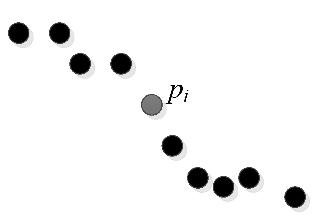
Figure 1.
A point and its k-neighboring points .

Figure 2.
Calculation of the local point cloud density.

Figure 3.
The test data: (a) point clouds named PC1 and (b) PC2 generated by deleting some points from PC1.
Figure 3.
The test data: (a) point clouds named PC1 and (b) PC2 generated by deleting some points from PC1.

Figure 4.
Results of experiment 1 (the results of 3D change detection varying the registration error through the approach using adaptive thresholds).
Figure 4.
Results of experiment 1 (the results of 3D change detection varying the registration error through the approach using adaptive thresholds).

Figure 5.
Qualitative comparison of 3D change detection at different misregistration of two point clouds (red points represent the change regions): (a) ground-truth of the change points and (b–d) results of change detection at the registration errors σ = 0.034 m, 0.048 m, and 0.069 m, respectively.
Figure 5.
Qualitative comparison of 3D change detection at different misregistration of two point clouds (red points represent the change regions): (a) ground-truth of the change points and (b–d) results of change detection at the registration errors σ = 0.034 m, 0.048 m, and 0.069 m, respectively.

Figure 6.
Results of experiments 2: (a–d) the results of the indicators completeness, correctness, quality, and F1, respectively, through these methods.
Figure 6.
Results of experiments 2: (a–d) the results of the indicators completeness, correctness, quality, and F1, respectively, through these methods.

Figure 7.
Qualitative comparison of 3D change detection via the three approaches. Red points represent change regions. (a) Ground-truth of change points; (b) results of change detection through “global”; (c) results of change detection via “local”; and (d) results of change detection via “adaptive”.

Figure 8.
Results of experiments 3: (a–d) the results of the indicators completeness, correctness, quality and F1, respectively, with varying number of neighboring points.
Figure 8.
Results of experiments 3: (a–d) the results of the indicators completeness, correctness, quality and F1, respectively, with varying number of neighboring points.


Table 1.
The accuracy of 3D change detection with different registration errors through the approach using adaptive thresholds.
Table 1.
The accuracy of 3D change detection with different registration errors through the approach using adaptive thresholds.
| Registration Error σ(m) | Completeness (%) | Correctness (%) | Auality (%) | F1 (%) |
|---|---|---|---|---|
| 0.048 | 95.78 | 93.71 | 90.01 | 94.74 |
| 0.055 | 95.74 | 84.19 | 81.15 | 89.60 |
| 0.062 | 95.74 | 74.64 | 72.22 | 83.88 |
| 0.069 | 95.58 | 62.73 | 60.96 | 75.75 |
Publisher’s Note: MDPI stays neutral with regard to jurisdictional claims in published maps and institutional affiliations. |
© 2021 by the authors. Licensee MDPI, Basel, Switzerland. This article is an open access article distributed under the terms and conditions of the Creative Commons Attribution (CC BY) license (http://creativecommons.org/licenses/by/4.0/).
Share and Cite
MDPI and ACS Style
Liu, D.; Li, D.; Wang, M.; Wang, Z. 3D Change Detection Using Adaptive Thresholds Based on Local Point Cloud Density. ISPRS Int. J. Geo-Inf. 2021, 10, 127. https://0-doi-org.brum.beds.ac.uk/10.3390/ijgi10030127
AMA Style
Liu D, Li D, Wang M, Wang Z. 3D Change Detection Using Adaptive Thresholds Based on Local Point Cloud Density. ISPRS International Journal of Geo-Information. 2021; 10(3):127. https://0-doi-org.brum.beds.ac.uk/10.3390/ijgi10030127
Chicago/Turabian StyleLiu, Dan, Dajun Li, Meizhen Wang, and Zhiming Wang. 2021. "3D Change Detection Using Adaptive Thresholds Based on Local Point Cloud Density" ISPRS International Journal of Geo-Information 10, no. 3: 127. https://0-doi-org.brum.beds.ac.uk/10.3390/ijgi10030127
Note that from the first issue of 2016, this journal uses article numbers instead of page numbers. See further details here.