Article

Spatiotemporal Analysis of COVID-19 Spread with Emerging Hotspot Analysis and Space–Time Cube Models in East Java, Indonesia

Department of Geography, Universitas Negeri Malang, Malang 65145, Indonesia
*
Author to whom correspondence should be addressed.
ISPRS Int. J. Geo-Inf. 2021, 10(3), 133; https://0-doi-org.brum.beds.ac.uk/10.3390/ijgi10030133
Submission received: 14 December 2020 / Revised: 26 February 2021 / Accepted: 1 March 2021 / Published: 3 March 2021

Abstract

:
In this research, we analyzed COVID-19 distribution patterns based on hotspots and space–time cubes (STC) in East Java, Indonesia. The data were collected based on the East Java COVID-19 Radar report results from a four-month period, namely March, April, May, and June 2020. Hour, day, and date information were used as the basis of the analysis. We used two spatial analysis models: the emerging hotspot analysis and STC. Both techniques allow us to identify the hotspot cluster temporally. Three-dimensional visualizations can be used to determine the direction of spread of COVID-19 hotspots. The results showed that the spread of COVID-19 throughout East Java was centered in Surabaya, then mostly spread towards suburban areas and other cities. An emerging hotspot analysis was carried out to identify the patterns of COVID-19 hotspots in each bin. Both cities featured oscillating patterns and sporadic hotspots that accumulated over four months. This pattern indicates that newly infected patients always follow the recovery of previous COVID-19 patients and that the increase in the number of positive patients is higher when compared to patients who recover. The monthly hotspot analysis results yielded detailed COVID-19 spatiotemporal information and facilitated more in-depth analysis of events and policies in each location/time bin. The COVID-19 hotspot pattern in East Java, visually speaking, has an amoeba-like pattern. Many positive cases tend to be close to the city, in places with high road density, near trade and business facilities, financial storage, transportation, entertainment, and food venues. Determining the spatial and temporal resolution for the STC model is crucial because it affects the level of detail for the information of endemic disease distribution and is important for the emerging hotspot analysis results. We believe that similar research is still rare in Indonesia, although it has been done elsewhere, in different contexts and focuses.

1. Introduction

COVID-19 first appeared in Wuhan City, Hubei Province, China, in December 2019 [1,2]. The disease is caused by Severe Acute Respiratory Syndrome Coronavirus 2 (SARS-CoV-2) [2]. More than 140 countries have confirmed cases and as a result, the disease has been categorized as a pandemic. As of 30 June 2020, the global total of confirmed cases reached 10,245,317, with 502,123 deaths [3]. COVID-19 cases began to be confirmed in Indonesia on 2 March 2020. As of 30 June 2020, there were 56,385 confirmed cases in Indonesia, with 2876 deaths. East Java was the most affected province, with a significant number of confirmed cases. As of 30 June 2020, the number of confirmed cases in East Java reached 11,932, with 893 deaths, and as a result, East Java has the largest total confirmed cases in Indonesia as of 30 June 2020 [4]. Based on this information, East Java is the ideal case study.
Research in China shows that the symptoms caused by COVID-19 vary from mild to severe symptoms. Examples of mild COVID-19 patients’ symptoms resemble the flu, namely cough and fever [5]. Severe symptoms are pneumonia, shortness of breath, Multi-organ Failure (MOF), even death [6]. These symptoms also appear in COVID-19 positive patients in Indonesia. The data collected regarding total COVID-19 cases in Indonesia shows that positive patients experience cough symptoms (70.3%), fever (46.6%), and shortness of breath (34%) [4]. Most cases of death from COVID-19 occur in patients with congenital diseases such as heart disease, diabetes, hypertension, and cancer, especially in those aged >60 years [7]. In Indonesia, there have been cases of death due to COVID-19 that are also caused by hypertension (5.76%), diabetes (5.07%), and heart disease (3.36%) [8].
The SARS-CoV-2 virus is spread through close contact and respiratory droplets [9]. Transmission can often occur in person-to-person environments, such as household and workplace activities [10]. This virus’ transmission process is also quite fast, as can be seen from the confirmed cases in Indonesia, which reached more than 1500 cases in the first 30 days [11]. The spread of the virus must be controlled immediately to limit the number of casualties. One way to inhibit the spread is to implement a physical distancing policy [12,13]. Each region has different characteristics, particularly meteorological and sociocultural characteristics, so the number of cases in each region varies. Liu et al. [14] report that meteorological characteristics such as environmental temperature, diurnal temperature, and absolute humidity play an independent role in COVID-19 transmission. Low temperatures, mild-diurnal temperatures, and low humidity tend to support transmission. These conditions improve the stability of coronavirus and support its transmission.
In contrast, other findings show that climate plays less of a role in virus transmission. Caspi et al. [15] report that warmer climates are negatively correlated with COVID-19 transmission rates but are more influenced by local transmission patterns. In essence, virus transmission is more dependent on time spent indoors vs. outdoors. Bhagat et al. [16] report that being indoors may increase the risk of contracting COVID-19 compared to being outdoors due to longer exposure times and decreased turbulence. Asyary and Veruswati [17] also reported that sun exposure is significantly correlated with the recovery of patients affected by COVID-19. Lack of UV-B rays exposure can lead to vitamin D deficiency in the body, potentially increasing the likelihood of infection by COVID-19 [18], which is also exacerbated by staying indoors.
Transmission of the SARS-CoV-2 virus can also be caused by sociocultural factors such as the absence of a sewer system in a particular area, worship places remaining open, crowds of people at entertainment venues at night, etc. Such differences certainly require different policies that consider the intensity of the increase in cases, e.g., physical distancing policies. Areas that experience a rise in cases apply stricter physical distancing policies compared to areas that experience an increase in cases. Spatiotemporal COVID-19 monitoring is one way to determine how COVID-19 cases are progressing in real-time based on the event’s place and time. Geospatial technology has grown rapidly and is utilized on local and global scales and has many applications. This technology’s reliability is undoubtedly the basis for its use in decision making, including in the case of COVID-19.
Geospatial technologies include Geographical Information System (GIS), Global Positioning System (GPS), and satellite-based Remote Sensing (RS) [19]. Geographical Information Systems have played an important role in many aspects of monitoring and tracking COVID-19 cases. GIS can dynamically monitor and track disease transmission using spatially placed technology as an effective visual communication tool [20,21]. One GIS use during the pandemic was creating map dashboards; however, detailed monitoring with GIS can be done using spatial analysis hotspots [22,23]. Hotspots are described as fixed entities or groups, e.g., geographical events or phenomena [24]. Hotspots are also only 2D and provide spatial information.
Newer approaches can provide 3D spatial information using immersive Virtual Reality (VR) with a spatial scale of 1:1 [25,26,27]. VR technology is also considered user-friendly because it can represent 3D spatial information more accurately than 2D [26]. In addition, head-mounted display-based VR with a wide field of view (FOV) can produce more immersive natural spatial perception [27]; however, VR technology is considered less suitable and not very useful in the representation of the thematic maps of endemic hotspots such as COVID-19, as it cannot accurately display the meaning and causation of detected hotspot patterns.
Moreover, Hruby et al. [25] proposed 3D visualization techniques, i.e., the geovisualization immersive virtual environments (GeoIVE), representing geospatial data in real-time; however, 3D visualizations for hotspot-based maps, especially maps used to illustrate COVID-19 distribution patterns, are still considered less suitable for real-time use, as COVID-19 transmission is difficult to physically determine due to human interaction and human mobility. The hotspot analysis can be represented with spatiotemporal data using a space–time cube (STC) model.
The definition of STC is a 3D visual form of a geographical phenomenon represented by the horizontal plane of the cube (spatial) and the vertical axis (time) represented in the bin [28]. Previous studies by Kveladze et al. [29] reported that the STC model could be used for geovisualization analytics to help users understand spatiotemporal patterns in commuter movement data. Marek et al. [30] report that the STC model’s use may explore the spatiotemporal trend of disease behavior caused by campylobacteriosis and can be visually focused onto a specific region; however, the problem with STC modeling lies in its visual complexity. Kveladze et al. [31] reported that the STC design makes it difficult for users to understand the meaning behind spatiotemporal data. Spatial aggregation techniques in one bin provide solutions to visual complexity, especially point-based data with output results in the form of hotspots that can accurately represent spatiotemporal data. Hotspots integrated with STC are referred to as emerging hotspot analysis. Both techniques can be used as tools for decision-making, especially for the handling of COVID-19 [32]. Building hotspots and STC require spatial data regarding the spread of COVID-19. Coronavirus transmission monitoring is critical so that we may detect areas that need serious treatment and help make predictions [33]. With monitoring, it is expected that COVID-19 can be handled effectively and efficiently.
Research on emerging hotspot analysis and STC for COVID-19 was previously adopted for a study conducted in China by Mo et al. [34]. Their analysis results mentioned that COVID-19 had spread rapidly and that transmission is centered in urban areas. STC models and emerging hotspot analysis have also been applied to other studies, e.g., the spatiotemporal characteristics of traffic accidents in elderly populations, gestational age and low birth weight at term, and hemorrhagic fever in renal syndrome epidemics [35,36,37]. STC and emerging hotspot analysis are becoming an increasingly popular trend in health studies because these approaches allow for spatiotemporal integration, which is important for disease surveillance and monitoring. Other research into COVID-19 transmission has also been conducted in Brazil, investigating metropolitan areas and along main roads with dense populations that feature significant amounts of hotspots [38]. This is the case with Desjardins et al. [2], who used space–time statistical models for COVID-19 monitoring in the United States. These researchers suggest quarantine or isolation measures to slow the transmission of the virus.
The transmission of the SARS-CoV-2 virus must be controlled immediately so that the number of casualties does not increase; one approach to reducing transmission is to map COVID-19 hotspots spatially. Previous research by Mo et al. [34] mapped COVID-19 transmission hotspots in China using the STC model, but hot/cold spot information uses all known data, so it has not been able to describe the spatial trend patterns of hotspot changes. There has been no research that examines the relationship between STC-based COVID-19 hotspots and proximity factors related to significant sites of interpersonal contact, such as entertainment venues, restaurants, transportation, and others. In addition, STC-based COVID-19 hotspot mapping has only been carried out in developed countries, not for developing countries such as Indonesia. It also does not address the possibility that the community’s mindset and culture do not impact the current COVID-19 outbreak, both in developed, developing, and underdeveloped countries; therefore, in this study, we aimed to (1) identify the trend pattern of STC-based COVID-19 hotspots with the time-to-time approach and overall time; (2) identify proximity factors strongly related to COVID-19 hotspots, especially in the East Java Province. This study’s results are expected to be considered by policymakers in determining decisions so the response to COVID-19 can be both effective and efficient.

2. Materials and Methods
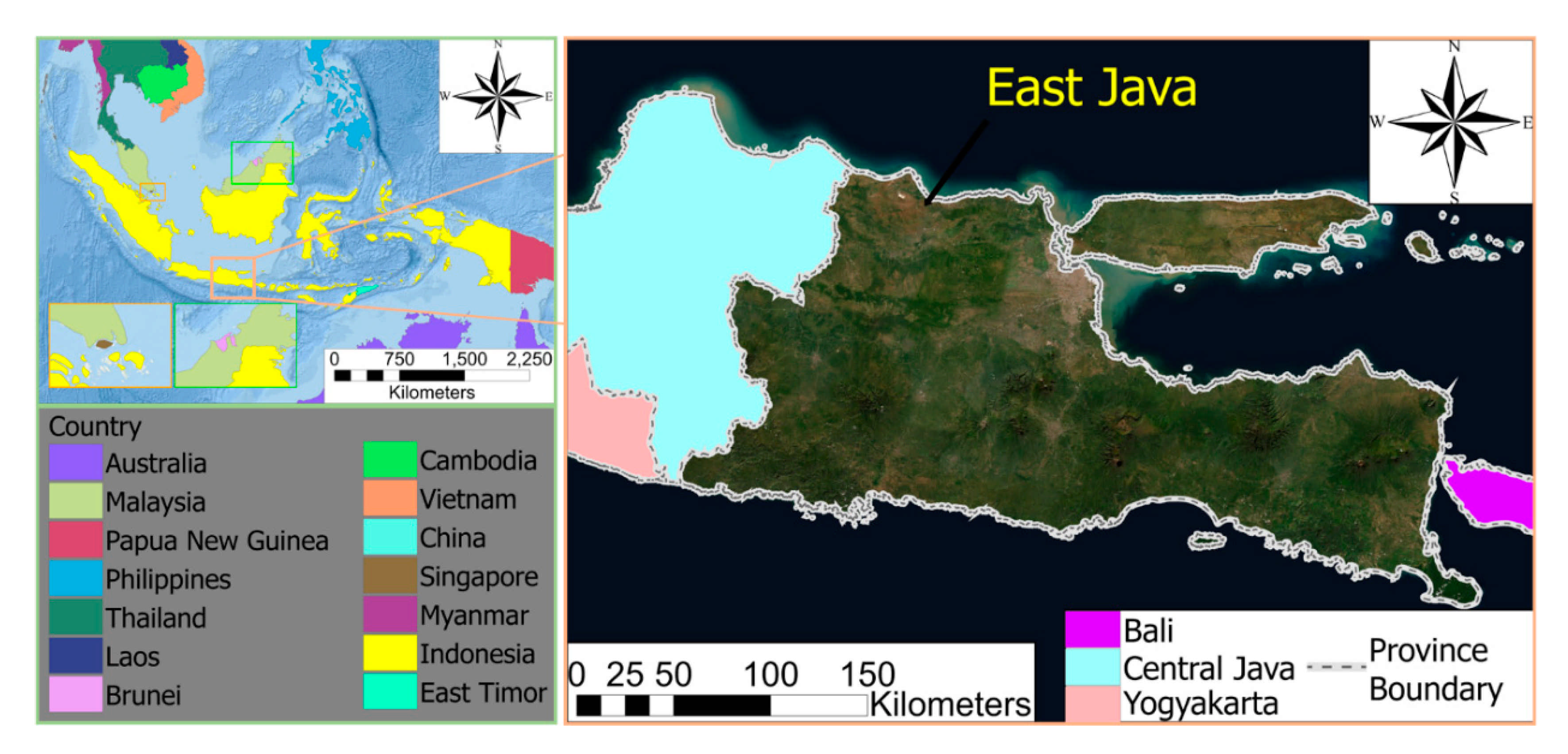
2.1. Study Area

East Java province is located at the eastern end of Java Island, Indonesia (Figure 1). The province was chosen as a research site because East Java is the second epicenter of the COVID-19 epidemic in Indonesia, after Jakarta. Within a few days, the number of positive cases in this region surpassed Jakarta. In terms of population, East Java is the second largest province in Indonesia after West Java. In the past decade, several endemic disease outbreaks have occurred in the region between 2009 and 2014, such as Dengue virus, Japanese encephalitis, and Chikungunya [39]. The uniqueness of this region’s social, economic, and cultural conditions is a strong reason for this research’s importance.

2.2. Data Source

Our data sources include the tracking of positive cases of the SARS-CoV-2 virus obtained from the COVID-19 Radar Website in East Java Province, including patients in care, recovery, and fatal cases [40]. Each case’s information consists of the point of the event location, the order of the case, the age, the gender, the patient’s status, the location of the village, the subdistrict, and the district. The coordinates of the positive case have low accuracy precision with a radius of 1 km and within the countryside’s scope, where the patient lives; the low precision was intentionally done in order to protect patient privacy. Spatiotemporal modeling was conducted using accumulated data over the last four months from mid-March, April, May, and June 2020 for a total of 9915 occurrences.

2.3. Analysis Method

We conducted two analyses in this study, which were nonspatial and spatial. The nonspatial analysis was conducted to describe the pattern of positive cases and deaths due to COVID-19 in East Java based on graphs integrated with demographic characteristics. The spatial analysis was carried out to identify COVID-19 hotspot patterns in East Java using maps to deepen knowledge regarding the distribution of COVID-19. The development of hotspot cluster models (2D and 3D) plot coronavirus cases spatially through a series of stages (Figure 2). The analysis process started with a tabulation of positive case event data in Microsoft Excel (CSV format). The data contain geo-referenced information on longitude and latitude coordinates (spatial dimensions) and time sequence events (time dimensions). The next step was to convert event data from a text file into an ESRI Shapefile through the ArcGIS Pro 2.5 software [41]. The spatiotemporal pattern analysis can be estimated using space–time cube (STC), along with an emerging hotspot analysis tool for spatial analysis. NetCDF data were visualized into 3D to determine the spatiotemporal trend. A hotspot pattern (emerging hotspot analysis) was then used for daily analysis each month (March, April, May, and June) to find trends over time.

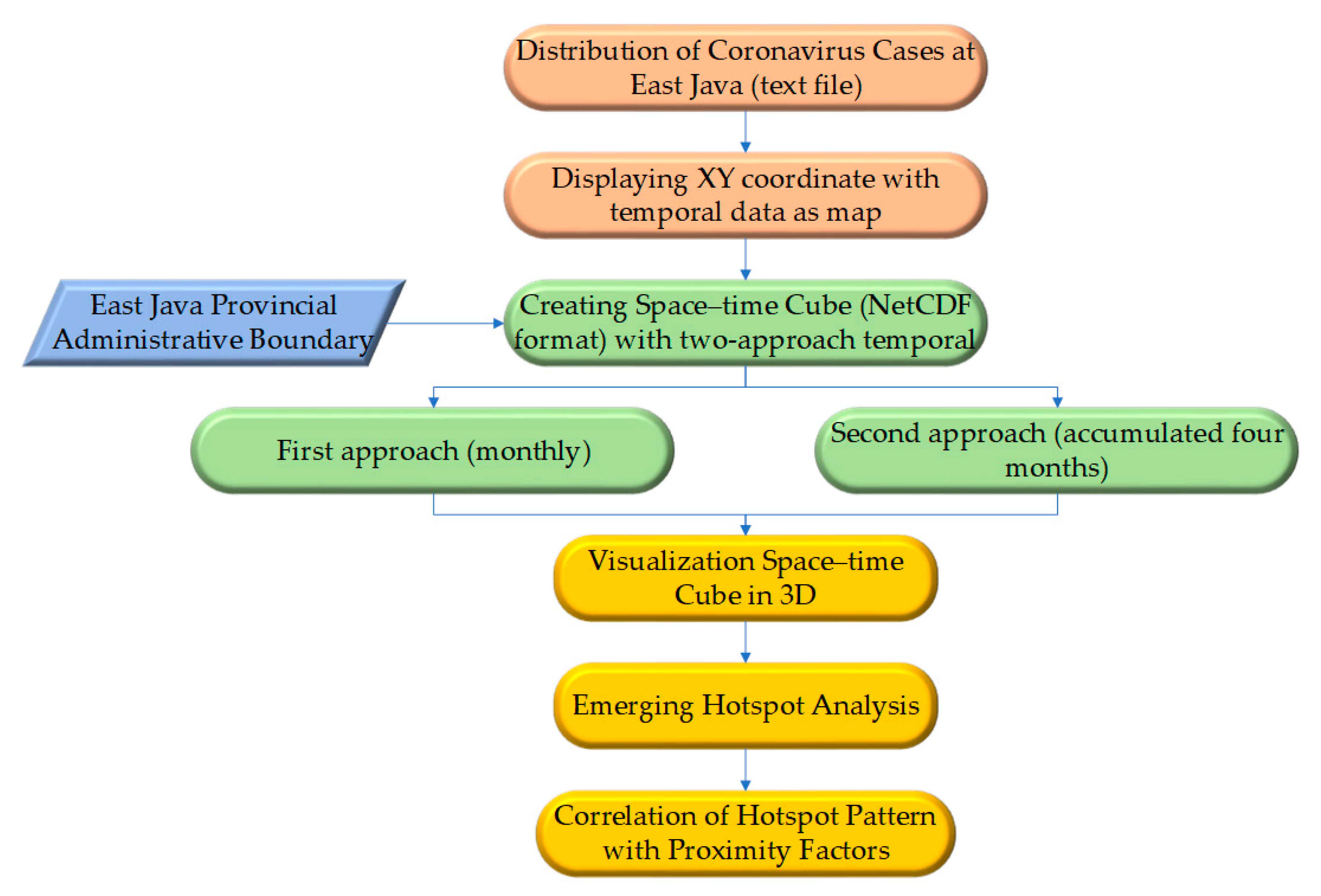
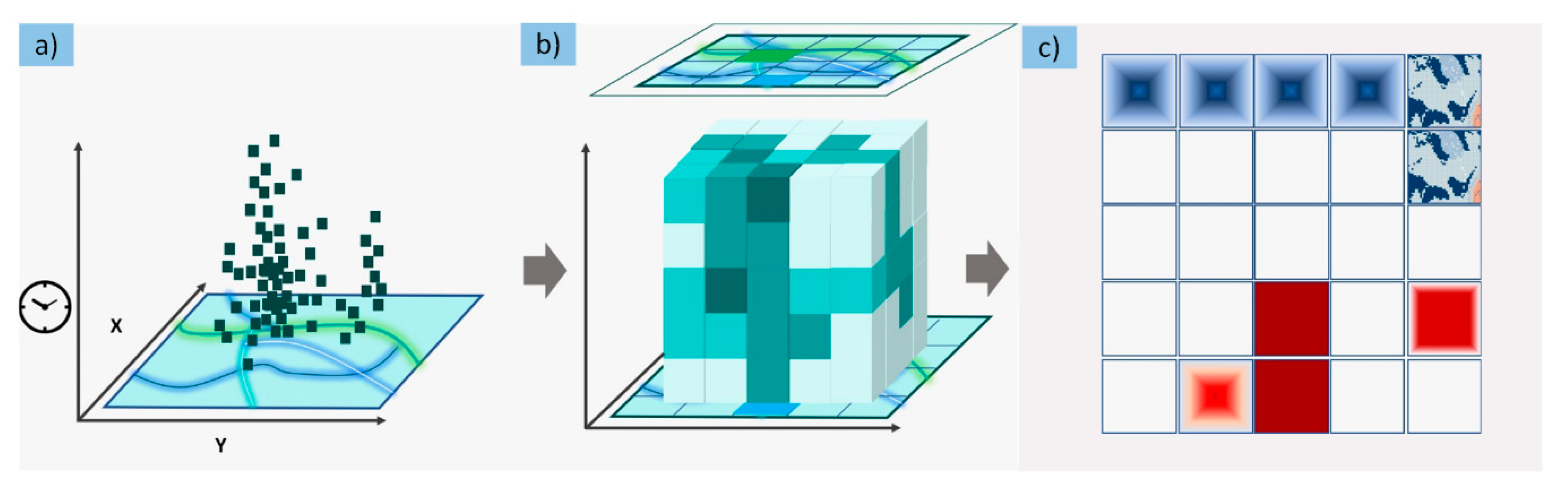
2.3.1. Spatiotemporal Analytics Framework

COVID-19 case data were used as STC input data. They were then converted to NetCDF data (Network Common Data Form), where x and y represent space dimensions, and t represents time dimensions. Columns that include the same region (x,y) have the same ID and can be integrated to represent the bin time series. In this study, the spatial size (x,y) in each bin was set at 1 km with a hexagonal bin (Appendix A: Figure A1) to match the accuracy of the location of positive cases of COVID-19 disease and the output of the provincial-scale map information. The calculated value of each bin reflects the number of occurrences at that location during a given time interval. The bin can be visualized in 3D geometry (Appendix A: Figure A2) on the computer screen through ArcGIS Pro.
We used two different approaches to identify the spread patterns of COVID-19 positive cases over time. In the first approach, the spatiotemporal distribution pattern of positive cases was analyzed monthly. In this analysis, we considered the number of cases that appear periodically, and the scale of mapping used in regional categories (provincial-scale); however, time step intervals are used daily starting when COVID-19 first entered East Java Province on 19 March 2020. The spatiotemporal distribution pattern was analyzed based on the accumulated time over the last four months of the same spatial size; however, time step intervals were used daily. Time Step Alignment was initially used because it follows the emergence of COVID-19 in East Java.

2.3.2. Emerging Hotspot Analysis

The hotspot analysis was intended to calculate the statistical significance of covering the regions with the highest spread of positive cases of COVID-19. In this study, using spatial (event location) and temporal (time of the event) hotspot analysis collected together into the bin is referred to as the emerging hotspot analysis (Appendix A: Figure A3) [42]. The time slice was set as an end time analysis based on the last month’s data, and the resulting STC is used as input data for hotspot analysis. There are two types of hotspot distribution patterns: hotspots with high-value significance over the entire period; cold spots where the significance of the value decreased over time [43,44].
Theoretically, hotspot analysis is based on the value of spatial relationships to calculate the statistics of each bin. We used Getis and Ord’s formula for emerging hotspot analysis given in Appendix B (Equations (A1) and (A2)) and the Conceptualization [45] of Spatial Relationships to create hotspot patterns using a fixed distance. These parameters relate to neighborhood distance and neighborhood time step. Neighborhood size affects cluster size in hotspots; small neighborhood distances produce variations in local trends; some features did not have neighborhood information [46,47]. Neighborhood distance value selection is a subjective element [48], so neighborhood distance was calculated automatically from the ArcGIS Pro software itself [47]. The optimal neighborhood distance value for two temporal approaches was 10 km; the neighborhood time step was 1.
Once the analysis of emerging hotspots was complete, each bin had a z-score, p-value, and hotspot classification. Furthermore, hotspot and cold spot trends were evaluated using the Mann–Kendall trend test [49,50]. The overall results of z-score and p-value hotspots and each bin’s trends can be classified into 17 categories given in Appendix C (Table A1 and Table A2) using the emerging hotspot analysis tool [44]. All bins with hotspot trends were evaluated using the Mann–Kendall trend test and hotspot trend analysis visualized in 2D.

2.3.3. Correlations of Hotspot Patterns with Proximity Factors

Hotspot connectivity patterns between regions were identified using hierarchical density estimates [51,52]. Hotspot location spreads were clustered based on high density and separated by low density. Hotspot objects with low density are considered noise or outliers. Clustering hierarchically can optimally maximize the overall stability of the selected cluster [52]. A grouping was then carried out based on a standard deviational ellipse [53] to identify the direction of distribution of density-based clustering results. Then, hotspot connectivity was determined between regions based on ellipse orientation.
We calculated the correlations of 13 proximity factors with the hotspot pattern to determine the potential association with the spread of COVID-19, including road density, distance to road, distance to the urban center, distance to automatic teller machines (ATMs), distance to attraction sites, distance to bank, distance to bus station, distance to cafe, distance to restaurant, distance to fuel station, distance to lodging, distance to rail stations, and distance to shopping centers and locations for a more in-depth interpretation related to hotspot connectivity patterns. All our proximity factors data were extracted from the Open Street Map (OSM) Website [54] and processed through ArcGIS Pro software. Then, we performed a zonal statistics analysis based on the hotspot/cold spot detected in East Java during either the first or second approach. An correlation ratio (Eta) was used to identify the relationship between hotspot/cold spot (nominal data) and proximity factors (numeric data). A correlation test was needed to reinforce assumptions about the spread of COVID-19 and hotspot connectivity patterns between regions. Classification of correlation values include weak correlation (≤0.35), modest correlation (0.36–0.67), strong correlation (0.68–0.9), and very strong correlation (≥0.9) [55].

3. Results

The results of this study are divided into four sections, including (1) analysis of temporal nonspatial data trend data and demographic characteristics of COVID-19 disease, (2) 3D visualization of STC models, (3) emerging hotspot analysis, and (4) correlations of hotspot patterns with proximity factors.

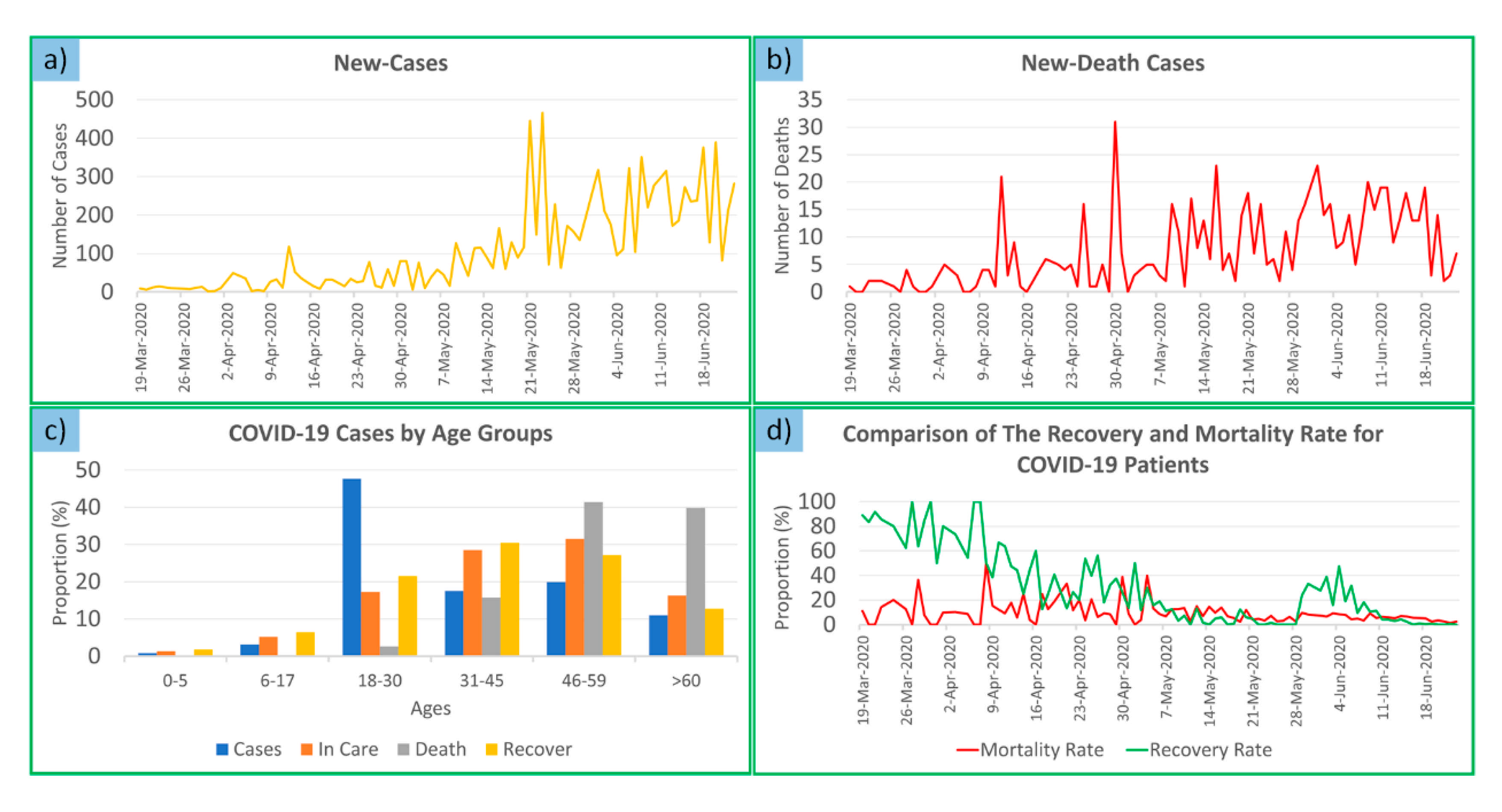
3.1. Analysis of Data on Nonspatial Trends and Demographic Characteristics of the COVID-19 Disease in East Java Province

The SARS-CoV-2 virus first appeared in East Java on 19 March 2020, and a total of nine people were confirmed positive. The patients came from three areas, namely Surabaya, Malang, and Malang Regency. The number of people infected with the virus increased over time. The data showed that 9915 people in East Java were infected with the SARS-CoV-2 virus from 19 March to 23 June 2020, with the death of 682 people and the recovery of 1188 people. The distribution of daily COVID-19 positive cases in East Java showed an increasing trend (Figure 3a). The initial emergence of COVID-19 from 19 March to 23 June 2020, shows a pattern between recovery and mortality rate (Figure 3d).
The COVID-19 pandemic curve from 19 March to 20 May 2020, shows an upward sloping trend, with a positive accumulative of cases in East Java, which included 2466 people; however, from 21 May to 23 June 2020, the trend of cases sharply increased. The spike in cases is clearer when analyzing the accumulative cases up to that date, which reached 9915 people, meaning East Java experienced a spike in cases of more than 7000 people in the space of a month, indicating that East Java’s coronavirus transmission rate was increasing faster since the end of May 2020.
The mortality curve in COVID-19 patients shows an increasing trend (Figure 3b), i.e., it does not experience a significant spike; this is evident from the cumulative case rate of COVID-19 patient deaths every month from March to June. In March, the cumulative death rate was 11 people; in April, 145 people; in May, 384 people; June of 682 people. The death rates show that the increase in COVID-19 patient deaths is not too sharp. The cumulative percentage of deaths was only 4.22% of the total positive confirmed cases (9915 cases).
The number of people infected with coronavirus ranges across different age groups (Figure 3c). The 0–5 age group has 123 cases, ages 6–17 has 485 cases, ages 18–30 has 7319 cases, ages 31–45 has 2692 cases, ages 46–59 has 3055 cases, and ages >60 has 1685 cases. The data show that patients with COVID-19 are mostly aged 18–30, whereas the 0–5 age group has the least number of positive cases.
The death rate of COVID-19 patients varies widely in each age group: age group 0–5 (one death), ages 6–17 (two deaths), ages 18–30 (17 deaths), ages 31–45 (102 deaths), ages 46–59 (268 deaths), and age >60 (258 deaths). Mortality rates in older adult groups account for the highest percentage of deaths relative to the total death count. The highest Case Fatality Rate (CFR) was 15.31%, indicating that the risk of death in elderly COVID-19 patients is quite high, even though the number of positive patients is not high.

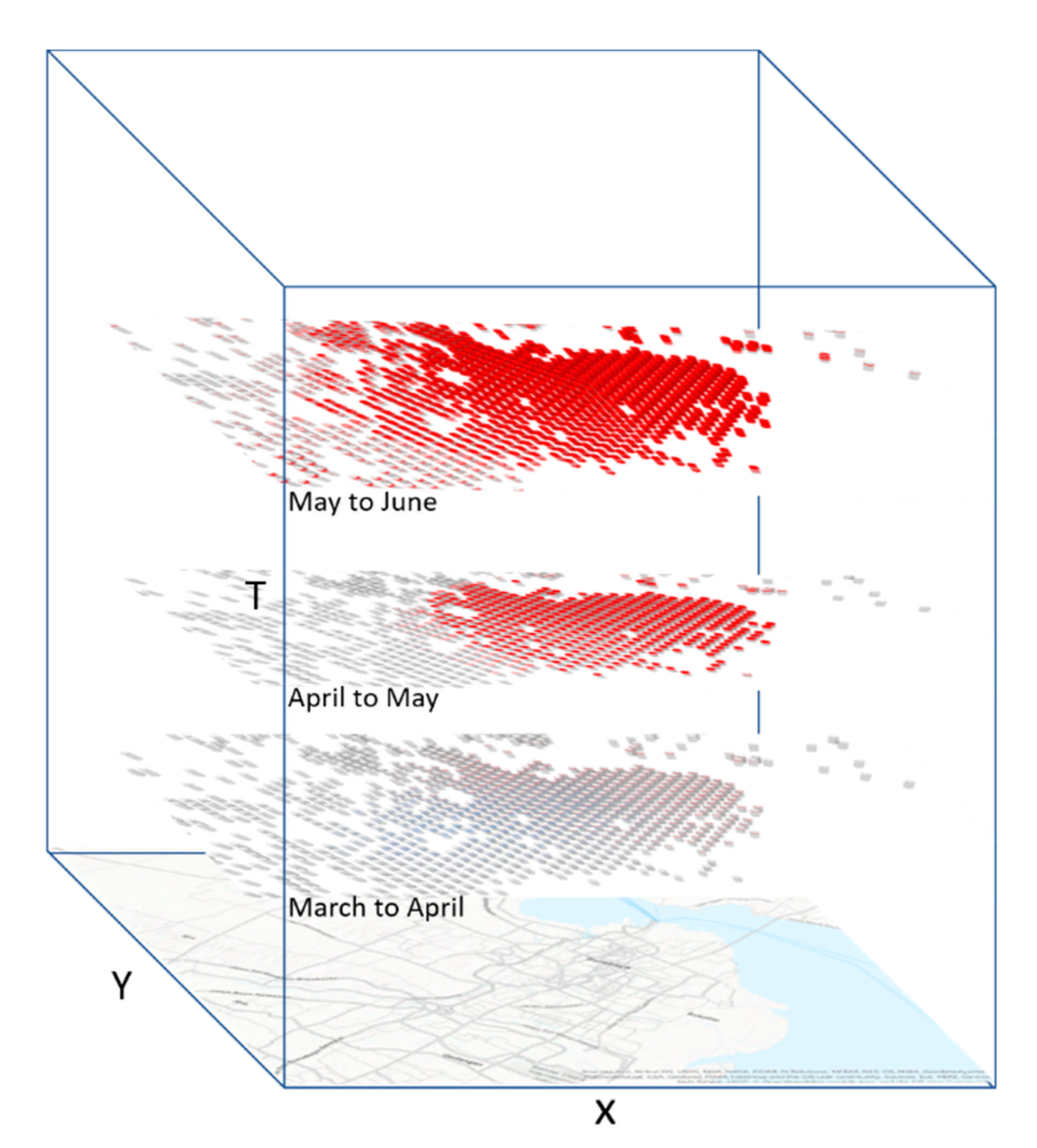
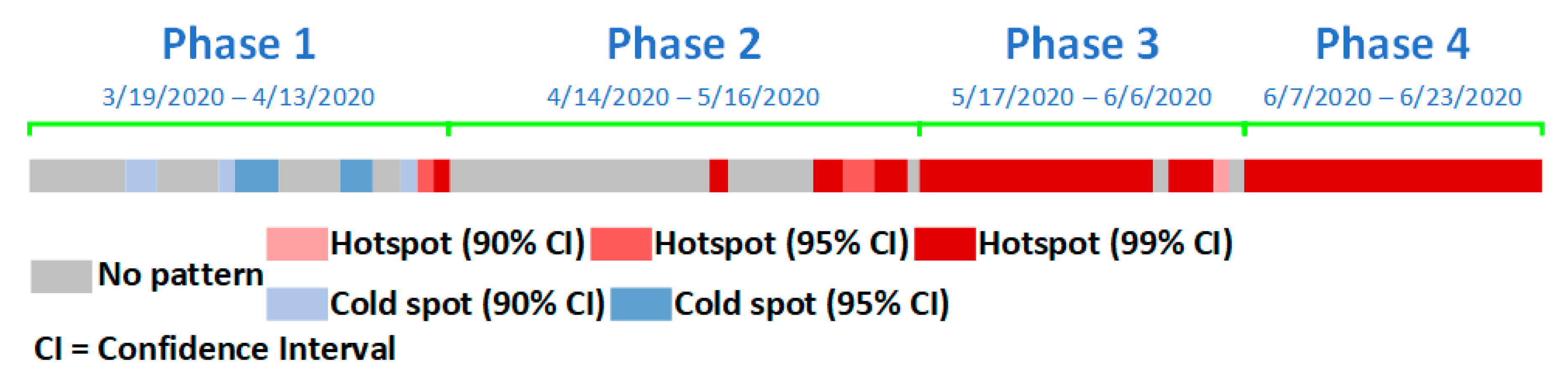
3.2. 3D Visualization of the STC Model for Hotspot Spatiotemporal Trend

The STC modeling was stored in NetCDF format and was visualized into three dimensions displayed in bin form (Figure 4), containing 84,002 grid locations with a spatial size of 1 km covering an area of 375.28 km from west to east and 194 km from north to south. The total number of STC bins is 8,148,194, which was gathered from the aggregation of the location and time of the occurrence of positive coronavirus cases in East Java. Mann–Kendall statistics were used to analyze and evaluate models on the overall case event trend data. The z-score = 9.3618 and p-value = <0.001 (<0.05), which means that the overall incidence rate of positive cases in East Java leads to an upward trend. Positive case incidents are displayed and classed based on hotspot trends of statistical significance: hotspots (99%, 95%, and 90% confidence), cold spot (99%, 95%, and 90% confidence), and no pattern (<90% confidence); however, STC is used to denote the area with the most significant hotspot trend, namely in Surabaya and surrounding areas (Figure 5).
The visualization results will be crowded if all available data were displayed and requires considerable computing resources. Figure 5a shows that cold spots were concentrated in the center of Surabaya in the first phase and spread to suburban areas, as the number of cases decreases every time with a significance of 90%–95% confidence interval (CI). Furthermore, there was an increase in new positive cases at the end of the second phase (Figure 5b), which visually indicated significant hotspots with a 95%–99% CI at the end of the bin. In the third phase (Figure 5c), there was a surge in cases in all areas of Surabaya and suburban areas; as such, significant hotspots appeared with an overall 99% confidence.
Figure 6 displays hotspot/cold spot patterns in a single bin representation at each time step interval. The interpretation of the hotspot/cold spot pattern based on time variability is divided into four phases. Phase division is not determined by a particular threshold but based on a significant change in hotspot/cold spot patterns. In phase 1, cold spots appear on-again and off-again. That is, a cold spot appears, then there is no pattern, and so on. Based on bin results, the z-score values in cold spots for confidence intervals (CI) of 90% and 95% are <–2.5 and −2.75–−2.5, respectively. At the peak of phase 1, there was an increase in trends marked by the emergence of hotspots with a CI of 95% then 99% with a value of z-score 2.78–3.3 and >3.3, respectively.
The classification of z-score values with a CI between 90% and 99% hotspots/cold spots is the same in each phase. In phase 2, there is no hotspot/cold spot 52% of the time, starting from the beginning of the phase; however, a hotspot appeared the next day with a CI of 99%. There are fluctuations in the pattern until the peak of the phase, where there is no pattern, then hotspots appear (99%, 95%, then 99%) inconsistently and end with no pattern. Hotspots with a CI of 99% consistently appear in phase 3, with at least 70% occurring since the beginning of the phase. The next day, no pattern appeared, and a hotspot with a CI of 99% appeared. Then, there is a decrease in hotspot trends to 90%, with a value of z-score of 2.5–2.78. At the peak of phase 3, no pattern appeared. Overall, in phase 4, hotspots consistently appear with a CI of 99% until the end of the phase. It can be noted that the bin representation described the hotspot/cold spot pattern at each time step interval in detail; we can alternatively directly explore COVID-19 cases spatially from any given time through hotspot analysis.

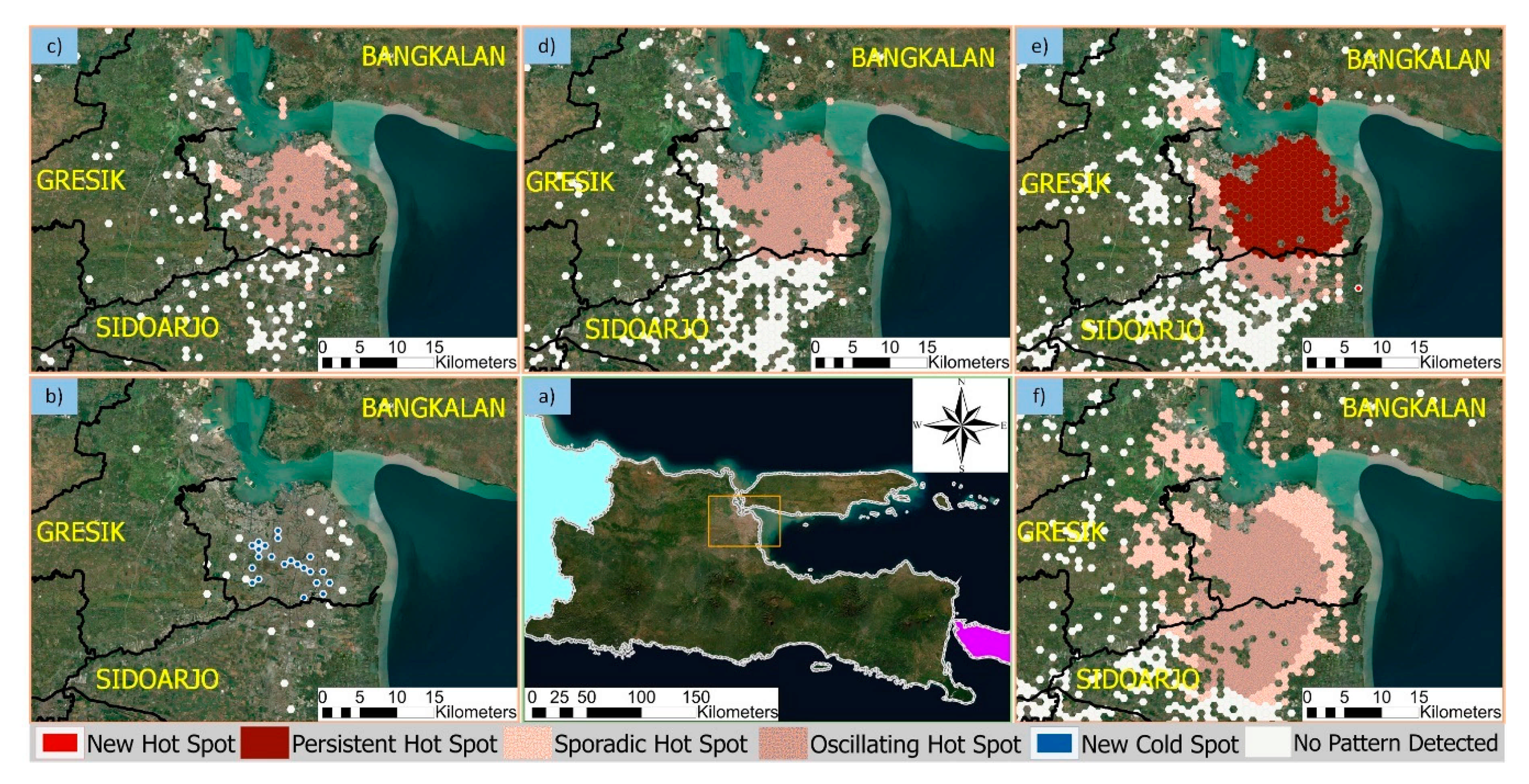
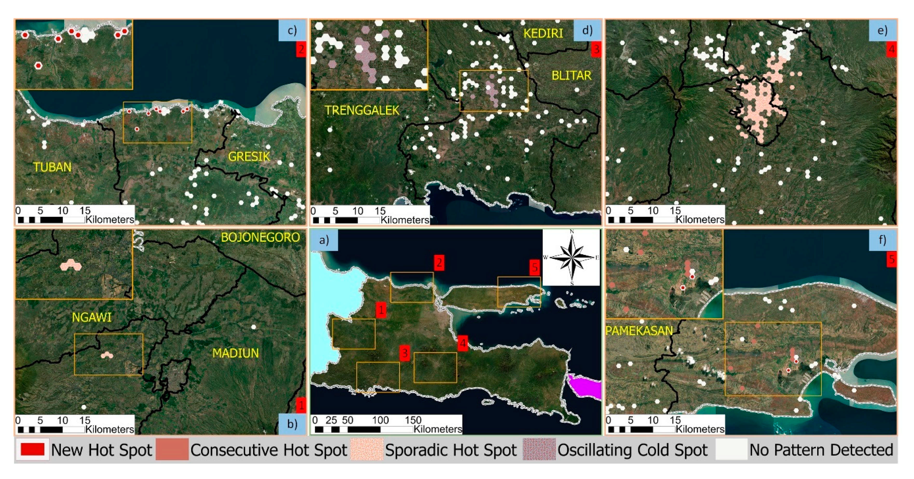
3.3. Emerging Hotspot Analysis (Monthly and Accumulated Four Months)

The hotspot analysis results show areas that have statistically increased or decreased in the number of cases. In the first approach, hotspots are created monthly. In March, as shown in Figure 7b, 22 new cold spots appeared in Surabaya Raya. In April (Figure 7c and Figure 8b), 123 oscillating and 30 sporadic hotspots appeared in Surabaya Raya, which were part of the largest cluster (Figure 7c) and a small part of the Magetan Regency (Figure 8b).
In May, hotspot patterns were detected in the Greater Surabaya area (Surabaya, Sidoarjo Regency, and Gresik Regency) and Malang Raya area (Malang City, Malang Regency, and Batu City); see Figure 7d and Figure 8c, respectively, for more information. There were 214 oscillating, 18 sporadic, three consecutive, and seven new hotspots in Lamongan Regency (Figure 8c). The hotspots were concentrated in Surabaya (Figure 7d) and slightly entered the Bangkalan Regency and Sidoarjo Regency.
There were 229 persistent, 53 sporadic, 77 oscillating hotspots in June, with 1 new hotspot and 12 oscillating cold spots (Figure 7e and Figure 8d). The number of cases increased continuously in the Surabaya city center area (Figure 7e) and spread widely towards the suburban area of Surabaya Raya. In Tulungagung Regency (Figure 8d), some local areas were cooling due to a decrease in positive cases.
The second approach of hotspot analysis uses the accumulation of coronavirus cases over a period of four months. Of course, the hotspot pattern will be different from the analysis results based on the time per month. There were 7 consecutive, 395 sporadic, 342 oscillating, and 2 new hotspots detected during March to June. There were two areas with large clusters, such as Surabaya Raya (Figure 7f) and Malang Raya (Figure 8e). Besides, several local areas in Sumenep Regency (Figure 8f) also appeared in new clusters. The entire coronavirus transmission process shown depends on the aggregation of the point location for four months; therefore, the spatiotemporal hotspot analysis in the second approach contains more general coronavirus cluster information than the first approach in terms of spatiotemporal data.

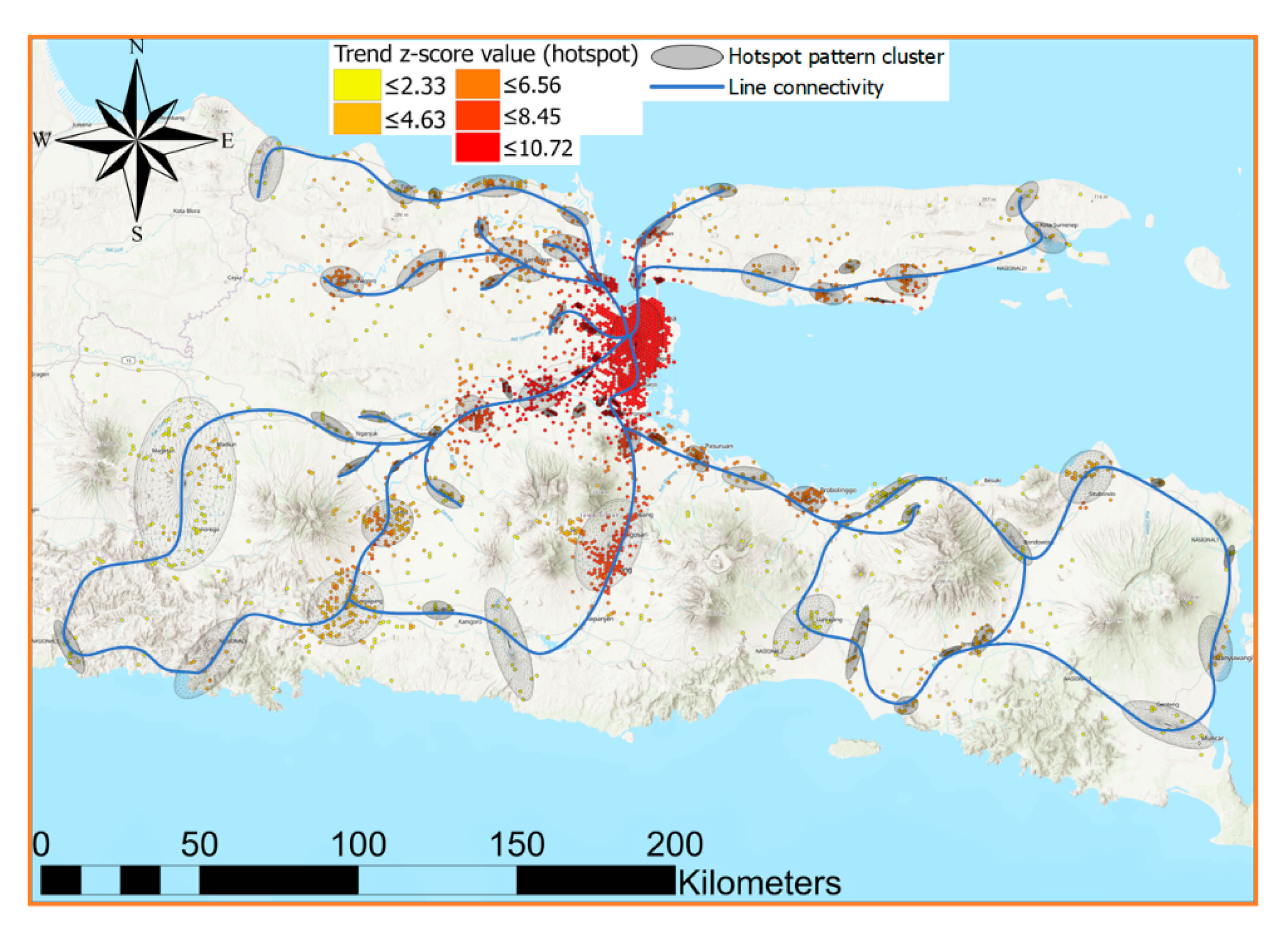
3.4. Correlations of Hotspot Patterns with Proximity Factors

The cluster of hotspots in the East Java Province from March to June is centered in Surabaya and its surroundings and closely related to the distance from the road and density of the road junction. Coronavirus transmission is directly affected by anthropogenic activity because, in general, coronavirus transmission occurs person-to-person through physical and air contact. Thus, a hotspot connectivity pattern was formed from the result of continuous inter-regional interactions. Hotspot connectivity patterns were built based on emerging hotspot analysis maps.
Figure 9 shows the hotspot connectivity pattern between regions, where the hotspots are shaped like an amoeba, with Surabaya city as the cluster center. Amoeba-shaped patterns indicate that coronavirus transmission is more likely to occur in city centers than in villages. The amoeba shape is based on the coronavirus cluster center, so that dots appear that form hotspot connectivity patterns continuously.
The correlation between hotspot pattern and 13 proximity factors is shown in Table 1. Overall, for the hotspots that were accumulated over a period of four months, there was a significant modest-level relationship with proximity factors, unless the distance to a bus station was at a weak level, as COVID-19 hotspots tend to cluster around places of commerce and business, financial storage, transportation, entertainment, and food, especially in urban areas with high road density. COVID-19 hotspots tend to cluster around these areas because the local population must all necessarily frequent these locations and services to meet their needs, leading to interaction with other people and risking the contraction of transmission of the virus; thus, the transmission of the virus is significant in urban areas. This situation also applies to COVID-19 hotspot relationships with proximity factors; however, among all modest-level relationships with COVID-19 hotspots, distance to the urban center, distance to fuel station, and distance to cafe factors fall into the highest category with correlation ratio (Eta) values of 0.639, 0.629, and 0.614, respectively.
Distance to a bus station has a weak relationship with COVID-19 hotspots. The possibility is logical because, at the time of the outbreak, restrictions were placed on services, e.g., a reduction in public transport, where the number of passengers was limited, routes and operating hours were limited, and physical distancing was imposed on buses in order to reduce transmission rates. Surprisingly, rail stations have a greater relationship with COVID-19 hotspots than bus stations, despite both enforcing service restriction policies. Logically, the difference in the level of relation to COVID-19 hotspots on bus and rail stations depends on population mobility, the ventilation quality factor, the cleanliness of the interiors of buses or trains, and the duration of travel time.
COVID-19 hotspots have a significant and consistent relationship with proximity factors, except for distance to bus stations in March; however, factors have a varying level of relationships over time, such as distance to road, road density, distance to the urban center, distance to ATMs, distance to attraction, distance to bus station, and distance to rail station. This situation indicates that the emergence of COVID-19 hotspots over time depends on the frequency of the population mobilizing to meet their needs, the adherence of residents to health protocols for COVID-19, and the effectiveness of government policies related to controlling the risk of COVID-19 outbreaks.

4. Discussion

At the time of this study, there were 9915 positive COVID-19 cases in East Java. Young people aged 18–30 accounted for the highest rate (7319); the highest mortality rate was found in ages 46–59 to >60. COVID-19 transmission patterns from March to June are marked by the changing patterns and dynamics of hotspots in every region in East Java. Surabaya and Malang are two cities that have sporadic and oscillating patterns. This condition is different from other cities in East Java, which only experience one or two sporadic patterns followed by cooling patterns.
Judging by the chart of the development of COVID-19 cases in East Java, it is clear that the number of daily cases tends to increase (Figure 3a). The government has made various efforts to prevent COVID-19 transmission, one of which is through the Large-scale Social Restrictions (PSBB). Implementation of the PSBB for the Surabaya Raya area, which became a hotspot area, was carried out in three phases from 28 April to 7 June 2020 [56]. The PSBB did not appear to reduce the curve in new cases significantly; the development of COVID-19 cases continued to increase during the PSBB period. This condition is due to the community’s poor adherence to health protocols such as physical distancing and masks [57,58].
The Surabaya Raya region began to enter the transition phase to “New Normal” from 8 to 22 June 2020, to restore economic conditions. During this phase, restrictions on economic activity were loosened while still adhering to health protocols. Since the end of the PSBB period, the number of daily COVID-19 cases in East Java has increased sharply, with an average of 250 daily cases; making East Java the province with the highest number of Indonesia’s cases and exceeding Jakarta on 20 June 2020 [4]. Although East Java has the highest number of cases in Indonesia, this province’s attack rate is not the highest in Indonesia. As of 27 June 2020, the value of the attack rate in East Java was ranked 9th out of the 34 provinces, with a value of 27, which means 27 per 100,000 residents of East Java were found to have COVID-19 [59]. Besides, East Java Province’s transmission rate as of 23 June 2020, is 1.0, meaning that every 5–7 days, each positive case will transmit one time [60]. The higher the transmission rate, the greater the potential for new cases to emerge.
The difference in method analysis used in previous studies lies in the type of aggregation form that serves to accommodate the number of positive case locations in a single bin. Previous research used a rectangular aggregation form with a 135 km2 grid size, such as the study by Mo et al. [34], whereas in this study, we used a hexagonal aggregation form. The shape of the hexagonal grid for ecological modeling analysis, especially in terms of connectivity, nearest neighborhood, and path movement, is lower in definition ambiguity than the rectangular grid [61]. In our study, the number of nearest neighbors to build STC and emerging hotspot analysis was the centroid, in a sense determined based on the fixed distance by using hexagon grids, which are superior to rectangular grids because more information is calculated [62]. There is no positive case sampling bias that would prevent neighbor information from tessellating (continuous and not overlap).
Temporal bias at one-day intervals in the STC model was close to the first and second averages above 30%. The last data point’s positive case data were directly omitted due to a drawback of the STC-based spatiotemporal analysis model. It is not easy to level the time interval on the spread of fluctuating positive cases of COVID-19 in one day. It is more appropriate to set the time step interval following the average incubation of the virus; however, it does not prevent the possibility of a small amount of temporal bias or a bias even higher than the one-day interval time step.
The neighborhood distance required to build the STC model, especially for COVID-19 cases, was calculated by default. This step is suitable for use because considering the transmission of viruses reviewed from the range of spread is so dynamic that it is difficult to determine the absolute value of neighborhood distance. Road density for proximity factors is set to the radius distance value by default. We considered it following the emerging hotspot analysis because road density and emerging hotspot analysis follow the regional scale mapping based on East Java province’s output extent.
Previous research by Wimberly et al. [63] focused on the West Nile virus (WNV) diseases based on dot density maps that are spatially smoothed. Their results showed that the Northern Great Plains region became a persistent hotspot of WNV, but there was no specific threshold value for hotspot classification. Mala and Jat [64] conducted a spatiotemporal analysis for the kernel density-based dengue disease and found that the kernel method can accurately represent the time dimension. From both studies, the STC model with over time and overall time approach can also help the spatiotemporal identification of hotspots in epidemic phenomena and be widely applied.
The 3D visualization on the STC model contains hotspot/cold spot COVID-19 pattern information on each bin detected in East Java. The information depends on the time step interval used. Each bin can be used to identify hotspot/cold spot significance value per time step interval. Of course, 3D visualizations can help see hotspot/cold spot change patterns in detail due to the aggregation of each bin’s positive case locations. Another advantage is that policymakers can monitor and evaluate policies applied at certain times in the bin related to policies and actions taken to prevent the spread of COVID-19; however, the downside of the 3D visualization of the STC model is that it cannot see each cube any deeper, and can only be seen from one side, making it difficult to understand and analyze the hotspot patterns. Emerging hotspot analysis can deduce the meaning of each bin’s hotspot pattern from 3D visualization results to facilitate an interpretation on a monthly and four-month accumulation of COVID-19 cases.
In the first approach, a decrease in cases of SARS-CoV-2 virus transmission in March in the Surabaya (new cold spot) area were due to the application of physical distancing areas, screening activities at intercity border locations, disinfectant spraying, tightening the policy of lane monitoring between city/district areas, and local lockdown of some areas. Transmission of the virus continued despite the implementation of PSBB; however, the emergence of new cases is uneven (sometimes appearing and disappearing) and occurred in sporadic hotspots because health protocols for preventing virus transmission were still implemented, e.g., the mandatory wearing of masks when in public, washing hands with hand sanitizer, physical distancing, and only leaving the house when necessary.
The PSBB event that was expected to reduce risk and break the transmission chain of the SARS-CoV-2 virus does not show significant results; we argue that many residents violated the night quarantine (9:00 p.m. to 4:00 a.m.), especially in Surabaya. Meanwhile, the emergence of positive cases is not so extreme and is interspersed with a decrease in the number of cases (cold spots) sometimes in a month represented by oscillating hotspots. New hotspots appear in Lamongan Regency, especially in pantura (north beach) settlements. Religious tourist attractions are officially closed by the local government, but not for some coastal tourist areas. As a result, the number of cases increased and the area became a new cluster (new hotspot).
New normal events in June resulted in an explosion in the number of positive cases, especially in Surabaya. The core area of the city became a persistent hotspot during this event because of the explosion of additional cases caused by the attack rate (189.3/100,000) and the horizontal rate of transmission (1.4) in Surabaya, which is categorized as high due to the close association and close contact of people [60]. This situation means that, for every 100,000 people, at least 190 of them are COVID-19 positive. The horizontal rate of transmission value exceeded 1, indicating that more and more people are infected over time, also due to the impact of the ‘new normal’ policy, i.e., the reopening of the country after quarantine measures; however, the new normal policy has taken into account health protocols, surveillance, and health system capacity. Tulungagung Regency showed oscillating cold spots, indicating that there were no new cases during the final two weeks in June, and patients recovered in some region clusters because there may not be any positive case reports from the end of the second to the third week of June; this could also be due to the incubation period of the virus, which is about 7–14 days.
Previous research has said that the prevalence of COVID-19 is higher due to the high percentage of older adults and weak health infrastructure [65]; however, in this study, we instead found that the countryside was more resistant to the SARS-CoV-2 virus, in contrast to the countryside in northeastern Brazil, which has a cluster of positive cases of COVID-19 [66]. The reasons for this difference include environmental conditions in the countryside, such as minimal pollutants, that are conducive to reducing the risk of developing chronic diseases that make somebody more prone to COVID-19 infection. Another possibility is that residents in rural areas have sufficiently strong immune systems and are less affected by the virus. In terms of economy, most rural areas become suppliers of food for urban areas (rice fields, horticultural crops, fishponds, marine fish, etc.). Rural residents also tend to keep their public activities local, which is likely to reduce the spread of transmission across the study period.
Transmission of the SARS-CoV-2 virus in East Java was more likely to occur in city centers. The amoeba-shaped pattern is centered in Surabaya and a metropolitan area in East Java Province’s capital. In this case, new findings emerged to explain the network of interactions, i.e., the accessibility of national roads connecting major cities played an important role in transmitting the virus, as social–cultural factors in Indonesia’s communities rely on traveling long-distance in close mobility using private vehicles. When people travel to other regions, they may be exposed to the virus. Besides, major cities have high intraurban connectivity, resulting in higher gross domestic product (GDP) values [67,68]; this results in more people using national roads and engaging in activities in the city. The transmission rate of the SARS-CoV-2 virus is higher because cities with high GDP indicate high economic activity and significant human interaction. This situation can be potentially emerging COVID-19 hotspots in the area.
Dense residential conditions with a high density of road network nodes, especially in urban areas, have high carbon emissions (PM2.5 and CO2) caused by the number of passing vehicles, leading to a higher risk of chronic diseases [69]; this may increase sensitivity to COVID-19 infection, which may mean that city residents could be at an increased risk compared to rural residents. Emissions are indirectly related to the emergence of hotspots due to poor air quality in the city; however, road density is inconsistent with COVID-19 hotspots in East Java every month. Moreover, places that fulfill the city’s primary needs in East Java, e.g., buying food in restaurants, gasoline for vehicles, and banks, consistently become hotspots due to human interaction through money, purchasing goods, and possible physical contact person-to-person. The night culture of East Java, e.g., cafe culture, is also a factor in the emergence of COVID-19 hotspot clusters. Lodging places are also consistently associated with hotspots due to the diverse factors of the people living there. In addition, the indoor conditions of urban buildings tend to be narrower and more poorly ventilated than large outdoor areas, making people who frequent the indoors more at risk of developing SARS-CoV-2 virus infection [70]. People in indoor areas also have to deal with long contact durations and person-to-person physical closeness; this also applies to buses and trains.
Our study has several limitations. One limitation is that the COVID-19 distribution coordinate plot data have low accuracy with a random location radius of 1 km, pattern depiction, and the spatial interaction between regions is subjective, especially clustering the emerging hotspot analysis results. We did not have access to any data that outlines a patient’s activities prior to testing positive, so the origin of SARS-CoV-2 virus transmission in East Java Province is unknown, as no contact tracing was performed. For future research, we first suggest that the neighborhood value for hotspot maps uses a stepwise approach (different sizes) for retail analysis. For support, the mapping should be based on a multiscale. Second, it is necessary to set the time step interval based on the virus’s incubation period in a multiclassification because each location’s incubation period may differ. Third, other proximity factors can be added related to coronavirus transmission, such as biophysical and anthropogenic factors, which can deepen the analysis that can later be useful to decision-makers who determine COVID-19 policy.

5. Conclusions

Spatiotemporal hotspot modeling using space–time cube (STC) and emerging hotspot analysis generates positive case location-based COVID-19 deployment pattern information. Three-dimensional hotspot visualization can represent changes in hotspot significance for every time step interval in each bin statistically. Different temporal phases can identify the direction of hotspot distribution that appears. The direction of hotspot distribution that appears in East Java is centered in Surabaya and the metropolitan area, which then spread widely to suburban areas and other cities over time. The drawback of 3D visualization is that it is difficult to determine the entire temporal hotspot pattern in each bin. To address this difficulty, emerging hotspot analysis is a useful analysis tool to identify the pattern. The irregular hotspot pattern describes a statistically significant hotspot for the last time step interval, which has a statistically significant cold spot during the previous time step. Less than 90% of time step intervals become statistically significant hotspots. Hotspot oscillating patterns denote locations that display an on-again–off-again pattern. Less than 90% of time step intervals become statistically significant hotspots, and no time step intervals become statistically significant cold spots. Both patterns occur in Surabaya Raya, which means the development of COVID-19 has been delayed or cured; however, the pattern is not balanced with the emergence of new cases, so that statistically, 90% is still significant. Hotspot analysis of the first approach, which was done monthly, has higher spatiotemporal information detail than the second approach (accumulation of four months) because it can highlight where cases are increasing, rapidly increasing, and appearing, which cannot be identified only by the entire data collection. Overall, the determination of spatial and temporal resolutions for building STC needs to be emphasized because it affects the detailed analysis level, especially for exploring endemic disease behavior. Of course, it directly impacts the results of the emerging hotspot analysis.
The hotspot cluster ellipse built from the emerging hotspot analysis has a continuous pattern resembling an amoeba. COVID-19 hotspots in East Java tend to appear in urban areas with intensive human interaction such as trade and business facilities, financial storage, transportation, entertainment, and food venues. Human interaction is directly related to urban activities and proximity to main roads. Based on the study results, we conclude that an efficient and effective policy is needed, especially for young people (18–30 years) who are generally asymptomatic; the lifestyle of millennials is also a contributing factor, especially in Surabaya and Malang. The patterns and characteristics of COVID-19 hotspots in East Java will most likely not be the same as other regions due to the community’s sociocultural factors that indirectly affect the intensity of human interaction. Overall, the STC model results and emerging hotspot analysis can be directly linked to supporting factors such as proximity factors to explain why the hotspot appeared in the region and did not appear in other regions.

Author Contributions

Conceptualization, Purwanto Purwanto, Sugeng Utaya, Budi Handoyo and Syamsul Bachri; Formal Analysis, Purwanto Purwanto, Syamsul Bachri and Ike Sari Astuti; Methodology, Purwanto Purwanto, Sugeng Utaya, Ike Sari Astuti and Kresno Sastro Bangun Utomo; Project Administration, Purwanto Purwanto; Software, Kresno Sastro Bangun Utomo and Yulius Eka Aldianto; Writing—Original Draft Preparation, Purwanto Purwanto, Sugeng Utaya, Budi Handoyo, Syamsul Bachri and Ike Sari Astuti; Writing—Review and Editing, Purwanto Purwanto, Budi Handoyo, Syamsul Bachri and Ike Sari Astuti; Visualization, Kresno Sastro Bangun Utomo and Yulius Eka Aldianto. All authors have read and agreed to the published version of the manuscript.

Funding

Universitas Negeri Malang supported the research through PNPB with no. contract: 3.3.16/UN32/KP/2020, LP2M with no. contract: 4.3.281/UN32.14.1/LT/2020, and ESRI Indonesia Education Program with no. contract: #535377.

Acknowledgments

The authors would like to thank all contributors for their work in this research. We also extend our thanks to the Universitas Negeri Malang and ESRI Indonesia.

Conflicts of Interest

The authors declare no conflict of interest.

Appendix A

Figure A1. A rectangular grid (left side image) and hexagonal grid (right side image). Based on [62], modified.
Ijgi 10 00133 g0a1
Figure A2. Visualization 3D of STC. Based on [71], modified.
Ijgi 10 00133 g0a2
Figure A3. (a) Point data locations. (b) Generating STC with the output NetCDF format. (c) Running emerging hotspot analysis tool for generating hotspot with 17 possible classes. Based on [39], modified.
Ijgi 10 00133 g0a3

Appendix B

Equations (A1) and (A2). Getis and Ord’s formula
G i * = j n w i , j x j X ¯ j n w i , j S n j 1 n w i , j 2 j 1 n w i , j 2 n 1
X ¯ = j = 1 n x j n , S = j = 1 n x j 2 n X ¯ 2
where x j is the attribute value, j is w i , j the spatial weight value between and, i and j is the total number of n features.

Appendix C

Table A1. Hotspot categories based on [44].
PatternSymbologyDefinition
No Pattern Detected Ijgi 10 00133 i001No pattern detected
Intensifying Hotspot Ijgi 10 00133 i002Locations that become hotspots are statistically significant during 90% of time step intervals, including final time step intervals. The intensity of high clustering amounts in each time step increases overall and is statistically significant.
Persistent Hotspot Ijgi 10 00133 i003Locations that become hotspots are statistically significant for 90% of time step intervals in the absence of trends indicating an increase or decrease in clustering intensity over time.
Oscillating Hotspot Ijgi 10 00133 i004A statistically significant hotspot for the last time step interval has a history as a statistically significant cold spot previously. Less than 90% of time step intervals have become statistically significant hotspots.
Sporadic Hotspot Ijgi 10 00133 i005The location of the hotspot is on-again rather than off-again. Less than 90% of time step intervals become statistically significant hotspots, and no time step interval is a statistically significant cold spot.
New Hotspot Ijgi 10 00133 i006The location is a statistically significant hotspot for final time step intervals and has never been a statistically significant hotspot before.
Diminishing Hotspot Ijgi 10 00133 i007Locations that become hotspots are statistically significant during 90% of time step intervals, including final time step intervals. The intensity of the high number of groupings at each time step decreased statistically significantly overall.
Historical Hotspot Ijgi 10 00133 i008The most recent period is not hot, but at least 90% of time step intervals have become statistically significant hotspots.
Consecutive Hotspot Ijgi 10 00133 i009Locations with one hotspot path are statistically significant without any interference in final time step intervals. Locations were never statistically significant hotspots before the last hotspot was run, and less than 90% of all bins were statistically significant hotspots.
Table A2. Cold spot categories based on [44].
PatternSymbologyDefinition
No Pattern Detected Ijgi 10 00133 i010No pattern detected
Intensifying Cold spot Ijgi 10 00133 i011Locations that become cold spots are statistically significant during 90% of time step intervals, including final time step intervals. The intensity of low clustering amounts at each step time increases overall and is statistically significant.
Persistent Cold spot Ijgi 10 00133 i012Locations that become cold spots are statistically significant during 90% of time step intervals in the absence of trends indicating an increase or decrease in clustering intensity over time.
Oscillating Cold spot Ijgi 10 00133 i013A statistical cold spot for the last time step interval has a history as a statistically significant hotspot during the previous step time. Less than 90% of time step intervals have become statistically significant cold spots.
Sporadic Cold spot Ijgi 10 00133 i014Cold spot location is on-again rather than off-again. Less than 90% of time step intervals become statistically significant cold spots, and no time step interval is a statistically significant hotspot.
New Cold spot Ijgi 10 00133 i015The location is a statistically significant cold spot for final time step intervals and has never been a statistically significant cold spot before.
Diminishing Cold spot Ijgi 10 00133 i016Locations that become cold spots are statistically significant during 90% of time step intervals, including final time step intervals. The low number-grouping intensity at each time step experiences a statistically significant overall decrease.
Historical Cold spot Ijgi 10 00133 i017The most recent period is not cold, but at least 90% of time step intervals have become statistically significant cold spots.
Consecutive Cold spot Ijgi 10 00133 i018Locations with one cold spot track are statistically significant without any interruptions in final time step intervals. Locations were never statistically significant cold spots before the last cold spot was run, and less than 90% of all bins were statistically significant cold spots.

References

  1. Huang, C.; Wang, Y.; Li, X.; Ren, L.; Zhao, J.; Hu, Y.; Zhang, L.; Fan, G.; Xu, J.; Gu, X.; et al. Clinical features of patients infected with 2019 novel coronavirus in Wuhan, China. Lancet 2020, 395, 497–506. [Google Scholar] [CrossRef] [Green Version]
  2. Desjardins, M.; Hohl, A.; Delmelle, E. Rapid surveillance of COVID-19 in the United States using a prospective space-time scan statistic: Detecting and evaluating emerging clusters. Appl. Geogr. 2020, 118, 102202. [Google Scholar] [CrossRef]
  3. Roser, M.; Ritchie, H.; Ortiz-Ospina, E.; Hasell, J. Coronavirus Pandemic (COVID-19)—Statistics and Research. Available online: https://ourworldindata.org/coronavirus (accessed on 10 August 2020).
  4. Gugus Tugas Penanganan COVID-19. Peta Sebaran COVID-19. Available online: https://covid19.go.id/peta-sebaran (accessed on 23 September 2020).
  5. Ruan, Q.; Yang, K.; Wang, W.; Jiang, L.; Song, J. Clinical predictors of mortality due to COVID-19 based on an analysis of data of 150 patients from Wuhan, China. Intensiv. Care Med. 2020, 46, 846–848. [Google Scholar] [CrossRef] [Green Version]
  6. Mahase, E. Coronavirus: Covid-19 has killed more people than SARS and MERS combined, despite lower case fatality rate. BMJ 2020, 368, m641. [Google Scholar] [CrossRef] [Green Version]
  7. Wu, Z.; McGoogan, J.M. Characteristics of and Important Lessons from the Coronavirus Disease 2019 (COVID-19) Outbreak in China: Summary of a Report of 72 314 Cases from the Chinese Center for Disease Control and Prevention. JAMA 2020, 323, 1239–1242. [Google Scholar] [CrossRef]
  8. Kemenkes, R.I. COVID-19 Dalam Angka per 3 Juli 2020. Available online: https://www.kemkes.go.id/article/view/20070500001/covid-19-dalam-angka-per-3-juli-2020.html (accessed on 23 September 2020).
  9. WHO. Advice on the Use of Masks in the Context of COVID-19; WHO: Geneva, Switzerland, 2020. [Google Scholar]
  10. De Ridder, D.; Sandoval, J.; Vuilleumier, N.; Stringhini, S.; Spechbach, H.; Joost, S.; Kaiser, L.; Guessous, I. Geospatial digital monitoring of COVID-19 cases at high spatiotemporal resolution. Lancet Digit. Health 2020, 2, e393–e394. [Google Scholar] [CrossRef]
  11. Kemenkes, R.I. Hindari Lansia Dari Covid 19. Available online: http://padk.kemkes.go.id/article/read/2020/04/23/21/hindari-lansia-dari-covid-19.html (accessed on 23 September 2020).
  12. Galvin, C.J.; Li, Y.-C.; Malwade, S.; Syed-Abdul, S. COVID-19 preventive measures showing an unintended decline in infectious diseases in Taiwan. Int. J. Infect. Dis. 2020, 98, 18–20. [Google Scholar] [CrossRef] [PubMed]
  13. WHO. Overview of Public Health and Social Measures in the Context of COVID-19; WHO: Geneva, Switzerland, 2020. [Google Scholar]
  14. Liu, J.; Zhou, J.; Yao, J.; Zhang, X.; Li, L.; Xu, X.; He, X.; Wang, B.; Fu, S.; Niu, T.; et al. Impact of meteorological factors on the COVID-19 transmission: A multi-city study in China. Sci. Total Environ. 2020, 726, 138513. [Google Scholar] [CrossRef]
  15. Caspi, G.; Shalit, U.; Kristensen, S.L.; Aronson, D.; Caspi, L.; Rossenberg, O.; Shina, A.; Caspi, O. Climate Effect on COVID-19 Spread Rate: An Online Surveillance Tool. medRxiv 2020. [Google Scholar] [CrossRef] [Green Version]
  16. Bhagat, R.K.; Wykes, M.S.D.; Dalziel, S.B.; Linden, P.F. Effects of ventilation on the indoor spread of COVID-19. J. Fluid Mech. 2020, 903, 1. [Google Scholar] [CrossRef]
  17. Asyary, A.; Veruswati, M. Sunlight exposure increased Covid-19 recovery rates: A study in the central pandemic area of Indonesia. Sci. Total Environ. 2020, 729, 139016. [Google Scholar] [CrossRef]
  18. Kohlmeier, M. Avoidance of vitamin D deficiency to slow the COVID-19 pandemic. BMJ Nutr. Prev. Health 2020, 3, 67–73. [Google Scholar] [CrossRef] [PubMed]
  19. Baker, T.R.; Battersby, S.; Bednarz, S.W.; Bodzin, A.M.; Kolvoord, B.; Moore, S.; Sinton, D.; Uttal, D. A Research Agenda for Geospatial Technologies and Learning. J. Geogr. 2014, 114, 118–130. [Google Scholar] [CrossRef] [Green Version]
  20. Saran, S.; Singh, P.; Kumar, V.; Chauhan, P. Review of Geospatial Technology for Infectious Disease Surveillance: Use Case on COVID-19. J. Indian Soc. Remote. Sens. 2020, 48, 1121–1138. [Google Scholar] [CrossRef]
  21. Sarfo, A.K.; Karuppannan, S. Application of Geospatial Technologies in the COVID-19 Fight of Ghana. Trans. Indian Natl. Acad. Eng. 2020, 5, 193–204. [Google Scholar] [CrossRef]
  22. Johns Hopkins University Coronavirus Resource Center. COVID-19 Dashboard by the Center for Systems Science and Engineering (CSSE) at Johns Hopkins University (JHU). Available online: https://0-coronavirus-jhu-edu.brum.beds.ac.uk/map.html (accessed on 29 October 2020).
  23. Saha, A.; Gupta, K.; Patil, M. Urvashi Monitoring and epidemiological trends of coronavirus disease (COVID-19) around the world. Matrix Sci. Medica 2020, 4, 121. [Google Scholar] [CrossRef]
  24. Songchitruksa, P.; Zeng, X. Getis–Ord Spatial Statistics to Identify Hot Spots by Using Incident Management Data. Transp. Res. Rec. J. Transp. Res. Board 2010, 2165, 42–51. [Google Scholar] [CrossRef]
  25. Hruby, F.; Castellanos, I.; Ressl, R. Cartographic Scale in Immersive Virtual Environments. KN J. Cartogr. Geogr. Inf. 2020, 1–7. [Google Scholar] [CrossRef]
  26. Lütjens, M.; Kersten, T.P.; Dorschel, B.; Tschirschwitz, F. Virtual Reality in Cartography: Immersive 3D Visualization of the Arctic Clyde Inlet (Canada) Using Digital Elevation Models and Bathymetric Data. Multimodal Technol. Interact. 2019, 3, 9. [Google Scholar] [CrossRef] [Green Version]
  27. Keil, J.; Edler, D.; Schmitt, T.; Dickmann, F. Creating Immersive Virtual Environments Based on Open Geospatial Data and Game Engines. KN J. Cartogr. Geogr. Inf. 2021, 1–13. [Google Scholar] [CrossRef]
  28. Kveladze, I.; Kraak, M.-J.; Van Elzakker, C.P. A Methodological Framework for Researching the Usability of the Space-Time Cube. Cartogr. J. 2013, 50, 201–210. [Google Scholar] [CrossRef]
  29. Kveladze, I.; Kraak, M.-J.; Van Elzakker, C.P. The space-time cube as part of a GeoVisual analytics environment to support the understanding of movement data. Int. J. Geogr. Inf. Sci. 2015, 29, 2001–2016. [Google Scholar] [CrossRef]
  30. Marek, L.; Tuček, P.; Pászto, V. Using geovisual analytics in Google Earth to understand disease distribution: A case study of campylobacteriosis in the Czech Republic (2008–2012). Int. J. Health Geogr. 2015, 14, 7. [Google Scholar] [CrossRef] [PubMed] [Green Version]
  31. Kveladze, I.; Kraak, M.-J.; Van Elzakker, C.P. Cartographic Design and the Space–Time Cube. Cartogr. J. 2018, 56, 73–90. [Google Scholar] [CrossRef]
  32. Paul, R.; Arif, A.A.; Adeyemi, O.; Ms, S.G.; Han, D. Progression of COVID-19 From Urban to Rural Areas in the United States: A Spatiotemporal Analysis of Prevalence Rates. J. Rural Health 2020. [Google Scholar] [CrossRef]
  33. Hohl, A.; Delmelle, E.M.; Desjardins, M.R.; Lan, Y. Daily surveillance of COVID-19 using the prospective space-time scan statistic in the United States. Spat. Spatio-Temporal Epidemiol. 2020, 34, 100354. [Google Scholar] [CrossRef]
  34. Mo, C.; Tan, D.; Mai, T.; Bei, C.; Qin, J.; Pang, W.; Zhang, Z. An analysis of spatiotemporal pattern for COIVD-19 in China based on space-time cube. J. Med. Virol. 2020, 92, 1587–1595. [Google Scholar] [CrossRef] [Green Version]
  35. Kang, Y.; Cho, N.; Son, S. Spatiotemporal characteristics of elderly population’s traffic accidents in Seoul using space-time cube and space-time kernel density estimation. PLoS ONE 2018, 13, e0196845. [Google Scholar] [CrossRef] [Green Version]
  36. Nielsen, C.C.; Amrhein, C.G.; Shah, P.S.; Aziz, K.; Osornio-Vargas, A.R. Spatiotemporal Patterns of Small for Gestational Age and Low Birth Weight Births and Associations with Land Use and Socioeconomic Status. Environ. Health Insights 2019, 13, 117863021986992. [Google Scholar] [CrossRef] [PubMed] [Green Version]
  37. Zhao, Y.; Ge, L.; Liu, J.; Liu, H.; Yu, L.; Wang, N.; Zhou, Y.; Ding, X. Analyzing hemorrhagic fever with renal syndrome in Hubei Province, China: A space–time cube-based approach. J. Int. Med Res. 2019, 47, 3371–3388. [Google Scholar] [CrossRef] [Green Version]
  38. Rex, F.E.; Borges, C.A.D.S.; Käfer, P.S. Spatial analysis of the COVID-19 distribution pattern in São Paulo State, Brazil. Ciência Saúde Coletiva 2020, 25, 3377–3384. [Google Scholar] [CrossRef]
  39. De Jong, W.; Rusli, M.; Bhoelan, S.; Rohde, S.; Rantam, F.A.; Noeryoto, P.A.; Hadi, U.; Van Gorp, E.C.M.; Goeijenbier, M. Endemic and emerging acute virus infections in Indonesia: An overview of the past decade and implications for the future. Crit. Rev. Microbiol. 2018, 44, 487–503. [Google Scholar] [CrossRef]
  40. East Java Government. East Java’s COVID-19 RADAR. Available online: https://radarcovid19.jatimprov.go.id/ (accessed on 30 June 2020).
  41. ESRI. ArcGIS Pro|2D, 3D & 4D GIS Mapping Software. Available online: https://www.esri.com/en-us/arcgis/products/arcgis-pro/overview (accessed on 23 January 2021).
  42. ESRI. Emerging Hot Spot Analysis (Space Time Pattern Mining)—ArcGIS Pro|Documentation. Available online: https://pro.arcgis.com/en/pro-app/tool-reference/space-time-pattern-mining/emerginghotspots.htm (accessed on 10 September 2020).
  43. Kondo, K. Hot and Cold Spot Analysis Using Stata. Stata J. Promot. Commun. Stat. Stata 2016, 16, 613–631. [Google Scholar] [CrossRef] [Green Version]
  44. ESRI. How Emerging Hot Spot Analysis works—ArcGIS Pro|Documentation. Available online: https://pro.arcgis.com/en/pro-app/tool-reference/space-time-pattern-mining/learnmoreemerging.htm (accessed on 11 September 2020).
  45. Ord, J.K.; Getis, A. Local Spatial Autocorrelation Statistics: Distributional Issues and an Application. Geogr. Anal. 1995, 27, 286–306. [Google Scholar] [CrossRef]
  46. Dubin, R.A. Spatial autocorrelation and neighborhood quality. Reg. Sci. Urban Econ. 1992, 22, 433–452. [Google Scholar] [CrossRef]
  47. ESRI. Modeling Spatial Relationships—ArcGIS Pro|Documentation. Available online: https://pro.arcgis.com/en/pro-app/tool-reference/spatial-statistics/modeling-spatial-relationships.htm#guid-f063a8f5-9459-42f9-bf41-4e66fbbcc415 (accessed on 10 September 2020).
  48. Harris, N.L.; Goldman, E.; Gabris, C.; Nordling, J.; Minnemeyer, S.; Ansari, S.; Lippmann, M.; Bennett, L.; Raad, M.; Hansen, M.; et al. Using spatial statistics to identify emerging hot spots of forest loss. Environ. Res. Lett. 2017, 12, 024012. [Google Scholar] [CrossRef]
  49. Mann, H.B. Nonparametric Tests Against Trend Author. Econometrica 1945, 13, 245–259. [Google Scholar] [CrossRef]
  50. Kendall, M.G. Rank Correlation, 4th ed.; Charles Griffin & Company Limited: London, UK, 1970. [Google Scholar]
  51. Kriegel, H.; Kröger, P.; Sander, J.; Zimek, A. Density-based clustering. Wiley Interdiscip. Rev. Data Min. Knowl. Discov. 2011, 1, 231–240. [Google Scholar] [CrossRef]
  52. Campello, R.J.G.B.; Moulavi, D.; Sander, J. Density-Based Clustering Based on Hierarchical Density Estimates; Springer: Berlin/Heidelberg, Germany; pp. 160–172.
  53. Yuill, R.S. The Standard Deviational Ellipse; An Updated Tool for Spatial Description. Geogr. Ann. Ser. B Hum. Geogr. 1971, 53, 28–39. [Google Scholar] [CrossRef]
  54. Open Street Map (OSM). Available online: https://www.openstreetmap.org (accessed on 6 July 2020).
  55. Taylor, R. Interpretation of the Correlation Coefficient: A Basic Review. J. Diagn. Med. Sonogr. 1990, 6, 35–39. [Google Scholar] [CrossRef]
  56. Toharudin, T.; Pontoh, R.S.; Zahroh, S.; Akbar, A.; Sunengsih, N. Impact of large scale social restriction on the COVID-19 cases in East Java. Commun. Math. Biol. Neurosci. 2020, 2020, 1–19. [Google Scholar] [CrossRef]
  57. Hasani, A. PSBB Fails to Flatten COVID-19 Curve in East Java: Task Force. Available online: https://www.thejakartapost.com/news/2020/05/08/psbb-fails-to-flatten-covid-19-curve-in-east-java-task-force.html (accessed on 24 September 2020).
  58. Isfandiari, M.A. Dua Penyebab Utama Kasus Covid-19 di Jawa Timur Terparah Hingga Melampaui DKI Jakarta. Available online: https://theconversation.com/dua-penyebab-utama-kasus-covid-19-di-jawa-timur-terparah-hingga-melampaui-dki-jakarta-142378 (accessed on 1 October 2020).
  59. Wicaksana, P. UNAIR Epidemiology Expert Explains Why East Java Become New Epicenter of Covid-19. Available online: http://news.unair.ac.id/en/2020/06/29/unair-epidemiology-expert-explains-why-east-java-become-new-epicenter-of-covid-19/ (accessed on 23 September 2020).
  60. Purba, D.O. Covid-19 di Jatim Tembus 10.092 Kasus, Waspada Attack Rate Surabaya Meningkat. Available online: https://surabaya.kompas.com/read/2020/06/24/05200071/covid-19-di-jatim-tembus-10092-kasus-waspada-attack-rate-surabaya-meningkat (accessed on 20 September 2020).
  61. Birch, C.P.; Oom, S.P.; Beecham, J.A. Rectangular and hexagonal grids used for observation, experiment and simulation in ecology. Ecol. Model. 2007, 206, 347–359. [Google Scholar] [CrossRef]
  62. ESRI. Why Hexagons?—ArcGIS Pro|Documentation. Available online: https://pro.arcgis.com/en/pro-app/tool-reference/spatial-statistics/h-whyhexagons.htm (accessed on 9 September 2020).
  63. Wimberly, M.C.; Giacomo, P.; Kightlinger, L.; Hildreth, M.B. Spatio-Temporal Epidemiology of Human West Nile Virus Disease in South Dakota. Int. J. Environ. Res. Public Health 2013, 10, 5584–5602. [Google Scholar] [CrossRef] [PubMed]
  64. Mala, S.; Jat, M.K. Geographic information system based spatio-temporal dengue fever cluster analysis and mapping. Egypt. J. Remote. Sens. Space Sci. 2019, 22, 297–304. [Google Scholar] [CrossRef]
  65. Cafer, A.; Rosenthal, M. COVID-19 in the Rural South: A Perfect Storm of Disease, Health Access, and Co-Morbidity; APCRL Policy Briefs; University of Mississippi: Oxford, MS, USA, 2020. [Google Scholar]
  66. Gomes, D.S.; Andrade, L.A.; Ribeiro, C.J.N.; Peixoto, M.V.S.; Lima, S.V.M.A.; Duque, A.M.; Cirilo, T.M.; Góes, M.A.O.; Lima, A.G.C.F.; Santos, M.B.; et al. Risk clusters of COVID-19 transmission in northeastern Brazil: Prospective space–time modelling. Epidemiol. Infect. 2020, 148, 1–23. [Google Scholar] [CrossRef]
  67. Derrible, S.; Kennedy, C. Characterizing metro networks: State, form, and structure. Transportation 2009, 37, 275–297. [Google Scholar] [CrossRef]
  68. Levinson, D.M. Network Structure and City Size. PLoS ONE 2012, 7, e29721. [Google Scholar] [CrossRef] [PubMed]
  69. Anenberg, S.C.; Achakulwisut, P.; Brauer, M.; Moran, D.; Apte, J.S.; Henze, D.K. Particulate matter-attributable mortality and relationships with carbon dioxide in 250 urban areas worldwide. Sci. Rep. 2019, 9, 11552. [Google Scholar] [CrossRef]
  70. Bouffanais, R.; Lim, S.S. Cities—Try to predict superspreading hotspots for COVID-19. Nat. Cell Biol. 2020, 583, 352–355. [Google Scholar] [CrossRef]
  71. ESRI. Create Space Time Cube by Aggregating Points (Space Time Pattern Mining)—ArcGIS Pro | Documentation. Available online: https://pro.arcgis.com/en/pro-app/latest/tool-reference/space-time-pattern-mining/create-space-time-cube.htm (accessed on 28 January 2021).
Figure 1. Research location in East Java, Indonesia.
Ijgi 10 00133 g001
Figure 2. Research workflow for 3D visualization of space–time cube (STC), emerging hotspot analysis, and correlation of hotspot pattern with proximity factors.
Ijgi 10 00133 g002
Figure 3. (a) The trend of confirmed nonspatial data on cases of COVID-19. (b) The trend of confirmed nonspatial data on the death of COVID-19 patients. (c) The number of COVID-19 cases based on age group proportion. (d) Comparison of the recovery and mortality rate for COVID-19 patients.
Ijgi 10 00133 g003
Figure 4. The STC design in a three-dimensional cube with x, y (spatial), and t (time).
Ijgi 10 00133 g004
Figure 5. A 3D visualization of STC for COVID-19 hotspots in Surabaya Raya. (a) Phase 1 from 19 March 2020 to 19 April 2020, (b) phase 2 from 19 April 2020 to 19 May 2020, and (c) phase 3 from 19 May 2020 to 23 June 2020.
Ijgi 10 00133 g005
Figure 6. Illustration of a bin representative that has hotspot and cold spot appearance patterns.
Ijgi 10 00133 g006
Figure 7. Hotspot/cold spot area detected in (a) Greater Surabaya in (b) March, (c) April, (d) May, (e) June, and (f) accumulated four months. Colors represent the degree of case severity (refer to Table A1 and Table A2 for color information).
Ijgi 10 00133 g007
Figure 8. Hotspot/cold spot area detected in (a) five areas, such as (b) Magetan in April, (c) Lamongan in May, (d) Tulungagung in June, (e) Malang Raya, and (f) Sumenep that accumulated over a period of four months, respectively. Colors represent the degree of case severity (refer to Table A1 and Table A2 for color information).
Ijgi 10 00133 g008
Figure 9. Amoeba-shaped hotspot connectivity pattern in East Java Province.
Ijgi 10 00133 g009
Table 1. Correlation ratio (Eta) between proximity factors and hotspot patterns.
Proximity FactorsMarchAprilMayJuneAll-Months
Dis-to-road0.361 *0.391 **0.330 **0.311 **0.382 **
Road density (km/km2)0.644 **0.688 **0.542 **0.435 **0.501 **
Dis-to-urban center0.601 **0.564 **0.708 **0.727 **0.639 **
Dis-to-ATMs0.309 **0.324 **0.568 **0.612 **0.495 **
Dis-to-attraction0.523 **0.378 **0.547 **0.302 **0.465 **
Dis-to-bank0.390 **0.512 **0.582 **0.665 **0.587 **
Dis-to-bus0.2210.371 **0.384 **0.655 **0.263 **
Dis-to-cafe0.527 **0.522 **0.579 **0.471 **0.614 **
Dis-to-restaurant0.465 **0.520 **0.582 **0.403 **0.589 **
Dis-to-fuel0.421 **0.573 **0.664 **0.630 **0.629 **
Dis-to-lodging0.502 **0.568 **0.450 **0.488 **0.578 **
Dis-to-rail0.414 **0.303 **0.613 **0.408 **0.437 **
Dis-to-shopping0.529 **0.568 **0.521 **0.589 **0.577 **
Note: ** = significance at the 0.01 level (two-tailed); * = significance at the 0.05 level (two-tailed); green color block = weak correlation; yellow color block = modest correlation; orange color block = strong correlation.
Publisher’s Note: MDPI stays neutral with regard to jurisdictional claims in published maps and institutional affiliations.

