Article

Near Real-Time Semantic View Analysis of 3D City Models in Web Browser

1
Department of Built Environment, Aalto University School of Engineering, P.O. Box 14100, FI-00076 Aalto, Finland
2
National Land Survey of Finland, Finnish Geospatial Research Institute FGI, Geodeetinrinne 2, FI-02430 Masala, Finland
*
Author to whom correspondence should be addressed.
ISPRS Int. J. Geo-Inf. 2021, 10(3), 138; https://0-doi-org.brum.beds.ac.uk/10.3390/ijgi10030138
Submission received: 4 January 2021 / Revised: 9 February 2021 / Accepted: 26 February 2021 / Published: 4 March 2021
(This article belongs to the Special Issue Virtual 3D City Models)

Abstract

:
3D city models and their browser-based applications have become an increasingly applied tool in the cities. One of their applications is the analysis views and visibility, applicable to property valuation and evaluation of urban green infrastructure. We present a near real-time semantic view analysis relying on a 3D city model, implemented in a web browser. The analysis is tested in two alternative use cases: property valuation and evaluation of the urban green infrastructure. The results describe the elements visible from a given location, and can also be applied to object type specific analysis, such as green view index estimation, with the main benefit being the freedom of choosing the point-of-view obtained with the 3D model. Several promising development directions can be identified based on the current implementation and experiment results, including the integration of the semantic view analysis with virtual reality immersive visualization or 3D city model application development platforms.

1. Introduction

3D city models depict the various components found in the urban environment, often containing both semantic and geometric information of these objects [1]. Commonly, such models are built following the CityGML specification and emphasize topologic and semantic aspects in addition to the geometry [2]. Other types of models have been applied as well, including, for example, large, textured meshes [3].
3D city models can serve as a starting point for both visualization and various analyses [4,5,6]. One of the most important applications of 3D city models has been the visualization for urban planning. The analysis potential of 3D city models also supports e.g., scenario development in urban planning [7]. Use of web-based 3D GIS tools for visualization and exploration of objects’ properties in a 3D city model have been strongly present in the research literature for a considerable amount of time [8,9]. The analyses that utilize 3D city models may rely solely on their three-dimensional geometry or complement this with the semantic information commonly included in these models. For example, the isovist analysis shown in [10] is mostly reliant on geometry, whereas the energy efficiency application in [8] also utilizes the semantic information of model objects. By integrating additional data sets to the 3D city model, analyses that combine the model geometry with various properties also become feasible (e.g., [5]).
Increasingly, the applications are implemented for web browsers, utilizing, e.g., virtual globes as a visualization tool for the 3D city model and may simultaneously contain tools for both user interaction and some analysis functionalities [11]. Service oriented architectures and server-side processes (e.g., server side rendering) have been suggested to improve performance on client devices that have limited computational capabilities [12]. Additional features have also been introduced to server-side visualization [13]. As the performance of consumer hardware has improved, it has become increasingly common to realize even the demanding applications directly in the browser, including both analysis and rendering tasks [14].
One of the central promises in 3D city modeling is that the same model would be applicable to a number of uses, and also support the development of new applications (e.g., [8]). As already stated, the application of 3D city models may occur either in computation and analysis use, using the models to produce new data (e.g., [15]) or by using the models as a platform for users’ processes, supporting user interaction [11]. This can include the use of models for supporting storytelling, in both journalistic [16] and artistic [17] sense. As the cities globally are taking up 3D city modeling, the development of new applications and tools that allow their use remains a topical research and development task. This is highlighted by the findings in [18]: despite the multitude of descriptions of 3D city model applications in the literature, it has been found that the actual 3D city modeling projects have occasionally fallen short from the envisioned broad applicability, even though this has been proclaimed as a major benefit of 3D city modeling.

1.1. 3D City Model Encoding Format CityJSON

CityGML has become one of the most important data models and formats for storing and exchanging 3D city models that contain both semantic and geometric information in digital systems [2]. In CityGML, the objects of the urban environment are depicted via a set of “thematic modules”, e.g., buildings or vegetation that can be further divided into specific features and represented in different levels of detail [2].
One of the currently ongoing developments in 3D city model formats has been the emergence of CityJSON, which aims to implement the data model of CityGML but in JavaScript Object Notation (JSON) encoding [19]. The authors argue that the benefits offered by the CityJSON encoding include the ease of parsing it in online systems (such as web browsers) that readily support the JSON encoding [19]. Furthermore, most of the programming languages are able to produce the required structures by combining two basic data structures, namely ordered lists and key-value pairs [19]. In addition to the development of the encoding format itself, various tools for producing CityJSON data have been developed and reported [20,21]. However, as the CityJSON is still a fairly new development, its use has not been extensively discussed in the literature yet, apart from few data integration applications [22].

1.2. View Analysis in Urban Environments

One of the applications in which the 3D model of the urban environment has proven beneficial is the analysis of visibility and views. This has been employed to a number of purposes, such as visibility estimation of landmarks in the urban environment for pedestrian navigation [23], evaluation of urban design scenarios [24,25] or property value estimation [26]. The related studies concerning real estate valuation and infill development are presented in Section 2.1.
It should be noted that, in addition to the examples utilizing a 3D model of the build environment as the starting point, somewhat similar types of visibility analyses have been performed from 2.5D datasets, like elevation models [27] or panoramic images [28]. While the benefits of 3D data for view analyses have been known for over two decades [29], visibility estimation and view analysis are not limited to 3D, and are currently perhaps more frequently used with photographic source data.
Frequently, the analyses concerning the visibility or what is seen from a certain position have focused on the visibility of individual objects (e.g., a landmark building in [23]), extent of the viewshed [26] or the visibility of certain object types such as unobstructed sky-view [24] or vegetation elements [25]. In view analysis concerning vegetation, a significant research track is the estimation of Green View Index (GVI) from photographic data sets. This is covered in more detail in Section 2.2.
One of the commonly applied technical principles in analyzing views is “pixel counting,” consisting of firstly utilizing a specific signal color for the element(s) of interest, obtaining an image (synthesized or real) from a chosen viewpoint and finally counting the number of signal colored pixels from the resulting image. An example implementation can be found from [23] utilizing a 3D urban model for producing synthetic images, and from [28] using panoramic photos of the real environment. When utilizing a 3D model, and obtaining the view for analysis via rendering, the pixel counting is simple to apply, as colors can be assigned to objects freely. When estimating the amount of pixels belonging to a certain category from a photograph, a system for determining which pixels belong to the wanted class is of course required first (e.g., for identification of vegetation pixels, see [30]).

1.3. Research Aims

As stated, the view analysis in the urban environment can support a number of applications, such as evaluation of the green infrastructure, real estate valuation, and infill development. In addition, a more general interpretation of views has been realized via deep learning and computer vision, used for classification of street scenes [31]. However, most past examples have relied on photographic, rather than model derived views, reducing their applicability in planning and comparing different development scenarios. In the examples where views derived from 3D models have been applied, the analyses have been focused on individual objects or object classes (such as designated buildings: [23] or green elements: [25]), not fully leveraging the semantic information present in contemporary 3D city models. Therefore, our aim is to implement a semantic view analysis, utilizing a 3D city model as source data and leveraging the semantic object information present in the model to obtain a better understanding of elements seen from a given viewpoint. The term semantic view analysis refers here to a view analysis that is able to determine what types of objects the user is seeing from a given viewpoint. In our implementation, the semantic information offered by a 3D city model, more precisely the model’s division to different types of city objects (e.g., buildings, roads, etc.), is utilized for obtaining this information. Furthermore, we implement the analysis as near real-time computation in a web browser, rather than as a pre-computed layer, as in some of the existing examples (e.g., [23]). The browser based implementation relying on the CityJSON format is presented.
As a prerequisite, the semantic view analysis requires a 3D city model describing as many visible components of the urban environment as possible. Ideally, this would be fulfilled by the existing 3D city models. However, many of the currently available 3D city models are typically focused on the buildings (for example, the CityGML model applied in the presented case only contained the bridge and building objects). Therefore, we present and apply a data integration pipeline for enriching the 3D city model with 2D map data, relying on the CityJSON format. With this, we achieve a model usable for the semantic view analysis. We present the data sets applied and the 3D city model obtained with the aforementioned data integration pipeline.
The analysis is tested in two alternative use cases, for which small experiments are provided. The first experiment demonstrates the use of the analysis for property valuation. The second experiment focuses on the urban green infrastructure evaluation. Here, the GVI obtained with the developed method is compared with a well-established panoramic image derived GVI. Based on the results, we discuss the limitations of the presented data integration pipeline and the semantic view analysis method. Finally, we present some of the emerging research and development topics.

2. Related Studies

2.1. Real Estate Valuation and Infill Development

The analysis of views in the urban environment is also utilized in the real estate sector, in particular for real estate valuation and infill development. In real estate valuation, this application relies on the assumption that the view from an apartment and the elements the view includes are some of the factors affecting the price of an apartment [25,26]. This is supported by evidence linking e.g., unobstructed sea views to property prices in high-rise residential development [26]. In the view analysis for valuation, the green views have also been touched upon. Ye et al. [32] showed that daily accessed visible street greenery holds significant positive coefficients for housing prices. The GVI or horizontal green view index (visual information on visible greenery gained from street view images using a pixel-level semantic segmentation) can be used as a parameter for property price prediction in hedonic price models (e.g., [28,33]). In research linking property valuation with green views, various permutations of the GVI have been introduced, including for example the floor specific green view index, introduced by [25]. In addition, the role of general environmental characteristics in residential housing prices has been studied through a combination of street view and remote sensing data [34]. Besides the perspective of developers’ pricing strategies, the view analysis via 3D models could potentially be utilized in the planning phase of redevelopment sites in order to maximize certain views (e.g., water and green elements) (see [26]).
One of the advantages of view analysis in real estate applications is its ability to obtain results that are specific to e.g., a certain individual window in a building. In infill development, the view analysis can be applied for assessing different infill development scenarios and their effects on the views from different apartments (see, e.g., [35,36]) and optimizing the design of the final scheme with respect to the green elements (see e.g., [33]). This is especially significant in the context of multi-owned housing. The apartment specific views become significant, as infill development often affects only views from some apartments, depending on the location of the new development (infilled building). Apartment owners affected the most by the infill development are worried about the possible value decrease of their apartments [37]. Thus, the disadvantages of the infill development are not equally distributed among the apartment owners, leading to questions about the property rights of the individual owners. Currently, there are no standardized tools to measure the impact of infill development on apartment values.
The use of view analysis derived from 3D models could assist with developing means to measure the impact of infill development on different apartments: how much the view changes regarding, e.g., greenery or water. This information could be used in developing compensation mechanisms within the multi-owned housing development (see, e.g., [37,38]).

2.2. Green View Index (GVI) on the Street Level

One of the urban elements frequently explored through the analysis of views has been the urban greenery. This is supported by a long research track highlighting the significance of views, and especially the presence of green elements in them, to human health, wellbeing and recovery [39,40,41,42]. The recent research on the urban green environment has promoted small-scale solutions, as they enable access to nature for urban residents more widely than larger and more concentrated urban green projects, and are likely easier to implement [43]. This also emphasizes the importance of street level views.
The most applied, though not completely unambiguous, metric for estimating the amount of greenery visible from a given point is the Green View Index (GVI), with one of the first examples being [44], utilizing GVI to evaluate the visibility of urban forest through a combination of field surveys and photography interpretation. Here, the GVI was estimated from a set of four non-overlapping images facing to four directions (north, east, west, south), first separating the pixels representing the greenery and then obtaining a single GVI value for the image acquisition point by averaging the results from the four pictures. In the past few years, GVI has been introduced in a variety of multidisciplinary urban studies and used along with data sets related to auditory experience [45], transportation choices [46], perceptual and cognitive experience [47,48], as well as walkability, movement, and health [42,49,50].
Panoramic images, such as those available from Google Street View (GSV), have become one of the most important sources for estimating the GVI, with several examples available [28,32,49,51,52,53]. In these cases, the GVI is typically not estimated from four non-overlapping images (as in [44]), but rather from a set of segments of the 360 degree panoramic image, with slightly varying implementations. In [28], a total of 18 sub-images are used for each position, obtaining images to six horizontal directions and three vertical directions for each heading. In [30,49], only the six images looking towards the horizon are used. Unfortunately, as in many cases, the camera opening angles are not disclosed (e.g., [28,30,49]), it becomes impossible to estimate the possible image overlap and the total coverage of the view analyzed. Therefore, it can be assumed that the GVI values obtained in different studies aren’t necessarily directly comparable. In addition to GSV, similar panoramic image sets from other providers have been applied [34,54,55].
Irrespective of the potential ambiguity of the GVI, it has been proven a useful metric for estimating greenery of the urban environment. In many cases, the GVI has been better in explaining certain observations concerning human welfare, when compared to conventional remote sensing metrics, such as the normalized difference vegetation index (NDVI) [56]. For example, the GVI (as derived from the street level panoramic images) has been found to correlate with recreational physical activity in the urban environment, unlike the NDVI (obtained from aerial images) [49]. A similar result was obtained in [41], noting that the satellite remote sensing derived green and blue (here referring to water surfaces) elements did not correlate with the depressive symptoms, but street view derived green and blue views did. These findings can potentially be explained by the ability of the street level GVI to offer a more human-scale viewpoint to the urban environment, when compared with the remote sensing based metrics. In some cases, this leads to mismatches between them. Larkin and Hystad [52] found the GVI to not correlate with satellite based NDVI. One of the possible explanations for these reported mismatches is that the GVI estimated from street views is unaffected by green elements present in courtyards or walled off areas, which do affect the green coverage estimates obtained from aerial imagery [48]. Kumakoshi et al. [57] conclude that the street view based GVI would be better suited to densely built urban settings than NDVI.

3. Materials and Methods
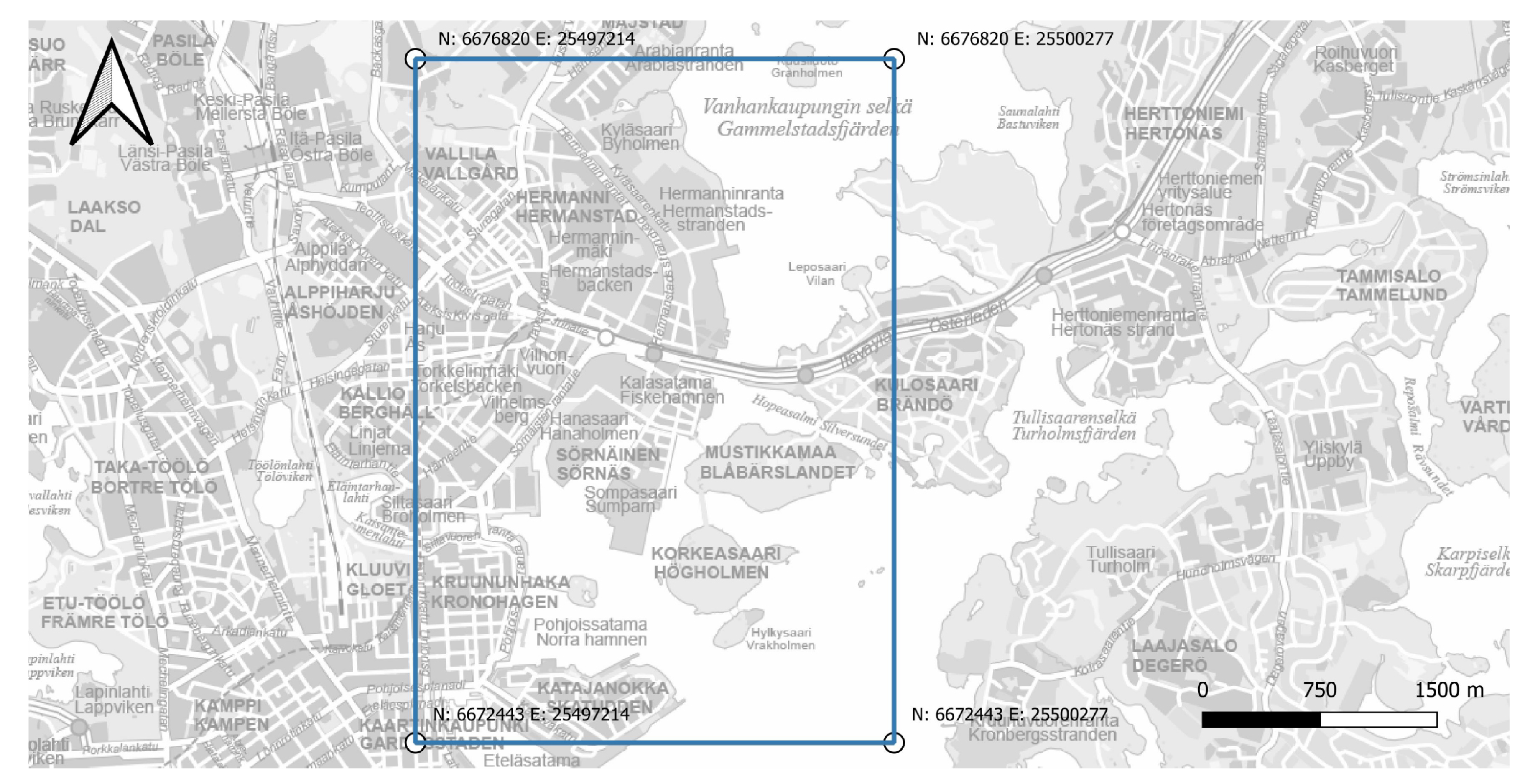
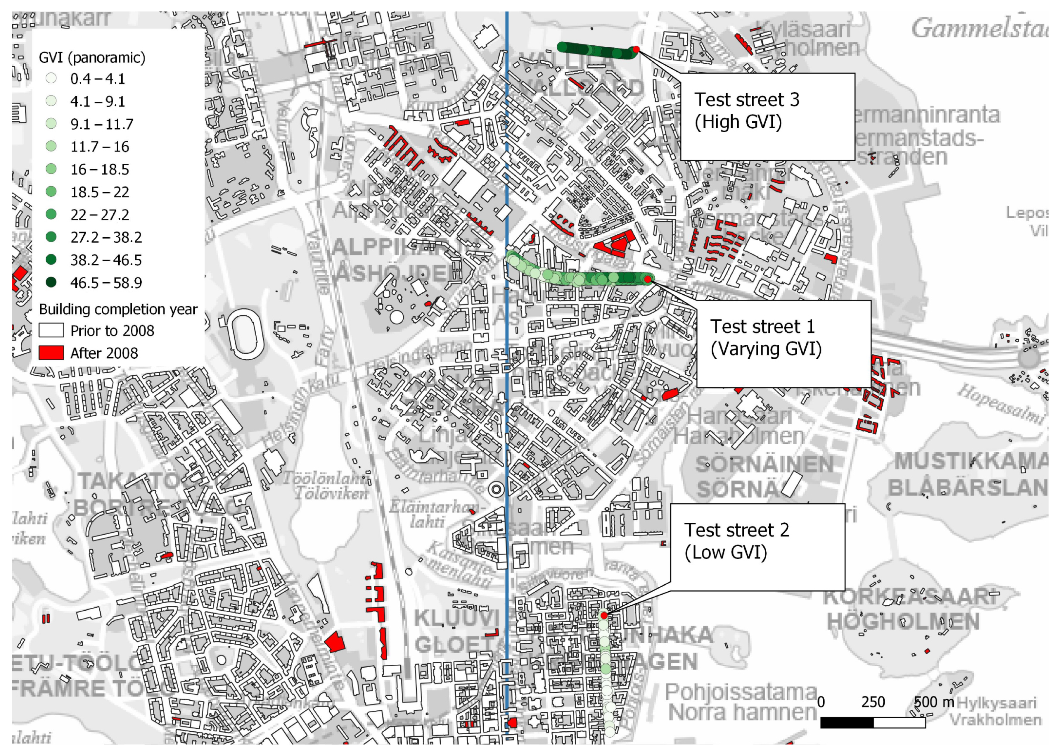
3.1. Test Site

The Kalasatama region of Helsinki, Finland was applied as a test site for view estimation. For data processing, a test site of approx. 3.0 by 4.3 km was used, totaling an area of 13.4 km2 containing a complex urban environment including a new high-rise development, major road and rapid transit connection, and varying amounts of urban green infrastructure (UGI). The position and extents of the test site are illustrated in Figure 1.

3.2. Datasets

The CityGML model of the Kalasatama area in Helsinki acted as the basis for producing the enriched model used in semantic view analysis. The model was supplanted with a set of map data, namely road and traffic area polygons, land cover classification polygons, and tree registry points. The digital elevation model (DEM) obtained from the National Land Survey of Finland, NLS (also available as open data) was used to provide elevation data for the map data. The applied datasets, their descriptions, and URLs are given in Table 1. The processing pipeline applied for integrating these with the CityGML building and bridge models is described in Section 3.3.
The green view index (GVI) data points, derived from Google Street View panoramic images, were used as a comparison data, as described in Section 3.5.2 This dataset and its production are described more in detail in [30].

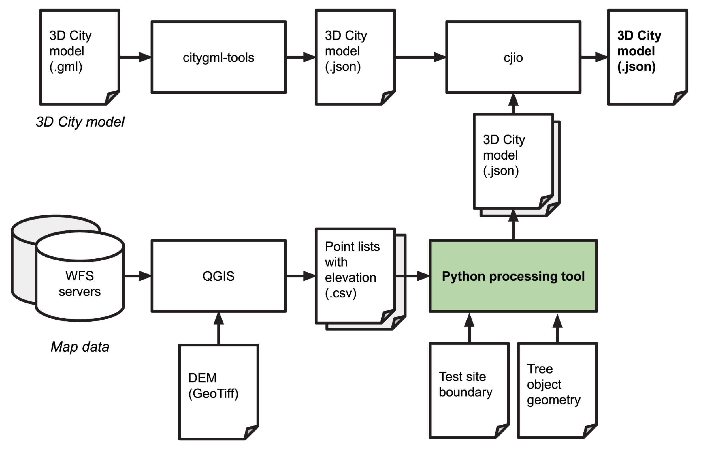
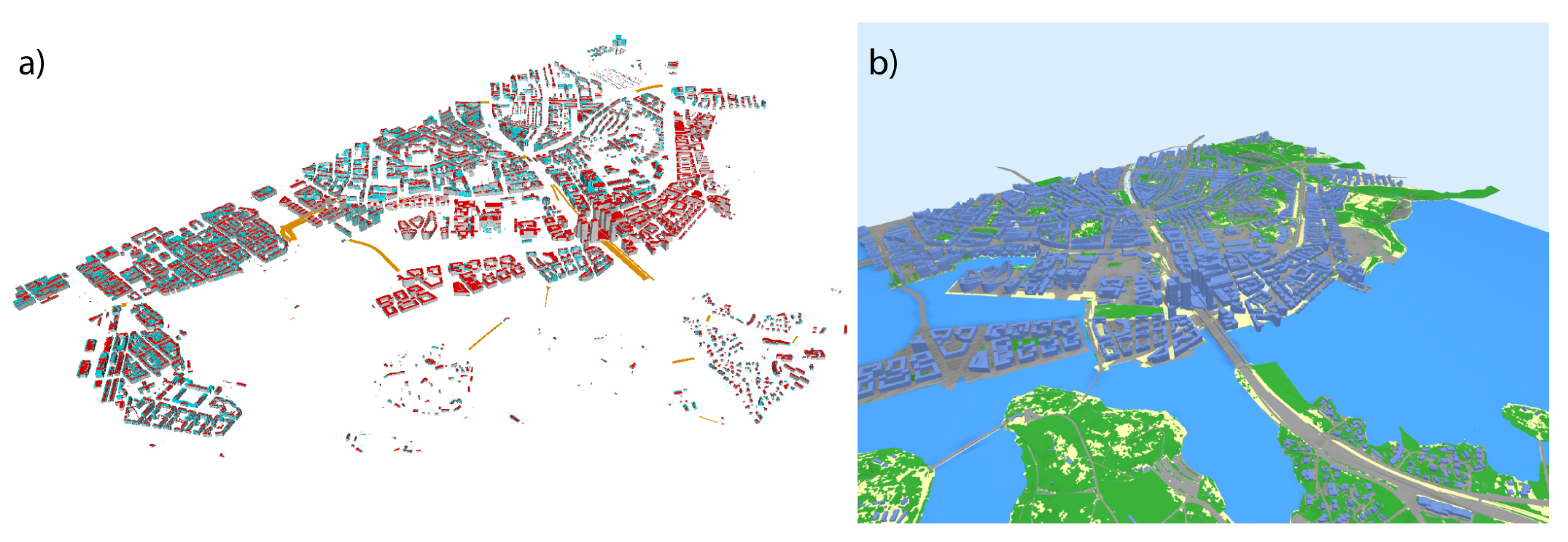
3.3. CityJSON Data Integration Pipeline

The idea of the integration pipeline was to combine the 3D city model and selected map data into an enriched 3D city model, using the CityJSON format. The integration consisted of converting the objects from different datasets (Table 1) to the same format, obtaining height information for the edges of originally two-dimensional objects and then including them in the same model. Objects were selected based on their group/class information (Table 2). The integration did not include estimating the suitability of individual objects with respect to their neighbors or filtering them, or modification of individual objects’ geometry to improve their fit.
As starting point, the CityGML building and bridge models were converted to CityJSON using the citygml-tools software [63] (version 1.3.2, Windows binaries). As the later visualization stages did not utilize the LOD1 depictions of buildings, they were excluded using the CityJSON/io—software “cjio” [64] (version 0.5.5).
The remaining datasets were obtained from the Web Feature Service (WFS) servers of the City of Helsinki and Helsinki Region Environmental Services Authority (HSY) using QGIS (version 3.4.2). For the 2D datasets without height information, the DEM from the National Land Survey of Finland was utilized to obtain heights using the Point Sampling Tool plugin [65] in the QGIS (version 3.4.2) software. After this, the polygonal areas with height information for each point of polygon were exported as comma separated values (CSV). The different object classes of the land cover classifications dataset were separated into classification specific files.
A python script (in Python 3.7.6) was developed to read the polygons from the CSV file, assemble them and their additional data into CityJSON data structure, and output the result as CityJSON file. An overview of the process is illustrated in Figure 2.
The land cover classification polygons were utilized to provide information for the areas not present in the 3D building models, road, and green area polygons. This includes e.g., those green areas that do not belong to city maintained parks but can be distinguished from aerial imagery, bare ground and bedrock and paved surfaces not belonging to the traffic area polygons. This was done to cover as much of the urban terrain as possible with objects, and thus achieve a hole-free description. The mapping from utilized data sets and their sub objects to CityJSON 1st level city objects (following the CityJSON 1.0.1 specification [66]) is given in Table 2. The CityGML to CityJSON conversion was allowed to also produce 2nd level city objects as present in the original data.
For the tree registry points, a simplistic pre-defined 3D model depicting a tree was utilized, the 3D symbol being scaled according to the stem width classes available in the city tree registry. The geometry was obtained by manually producing a mesh model in Blender 3D (2.90.1), exporting it as OBJ-file and then integrating the vertex geometry & face lists into the Python tools. In a similar manner, the information of the test area boundary was integrated into the processing tool. Finally, the CityJSON/io—software was used to merge the CityJSON files to obtain a single model.

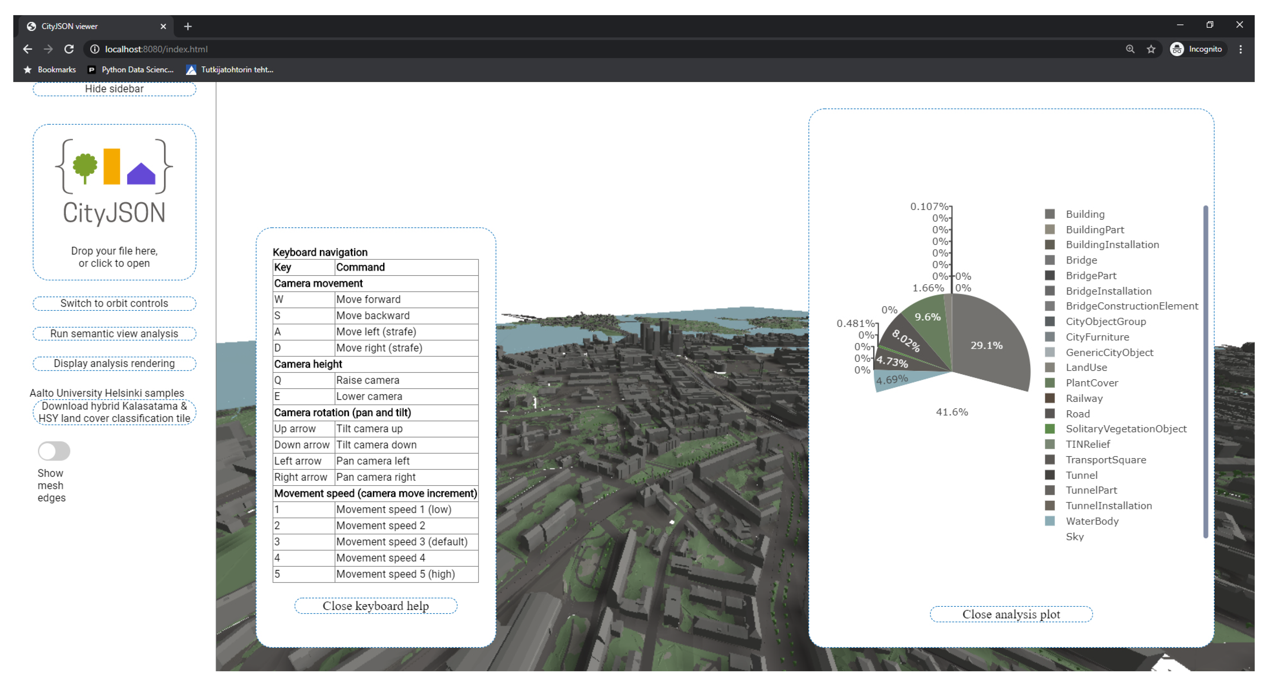
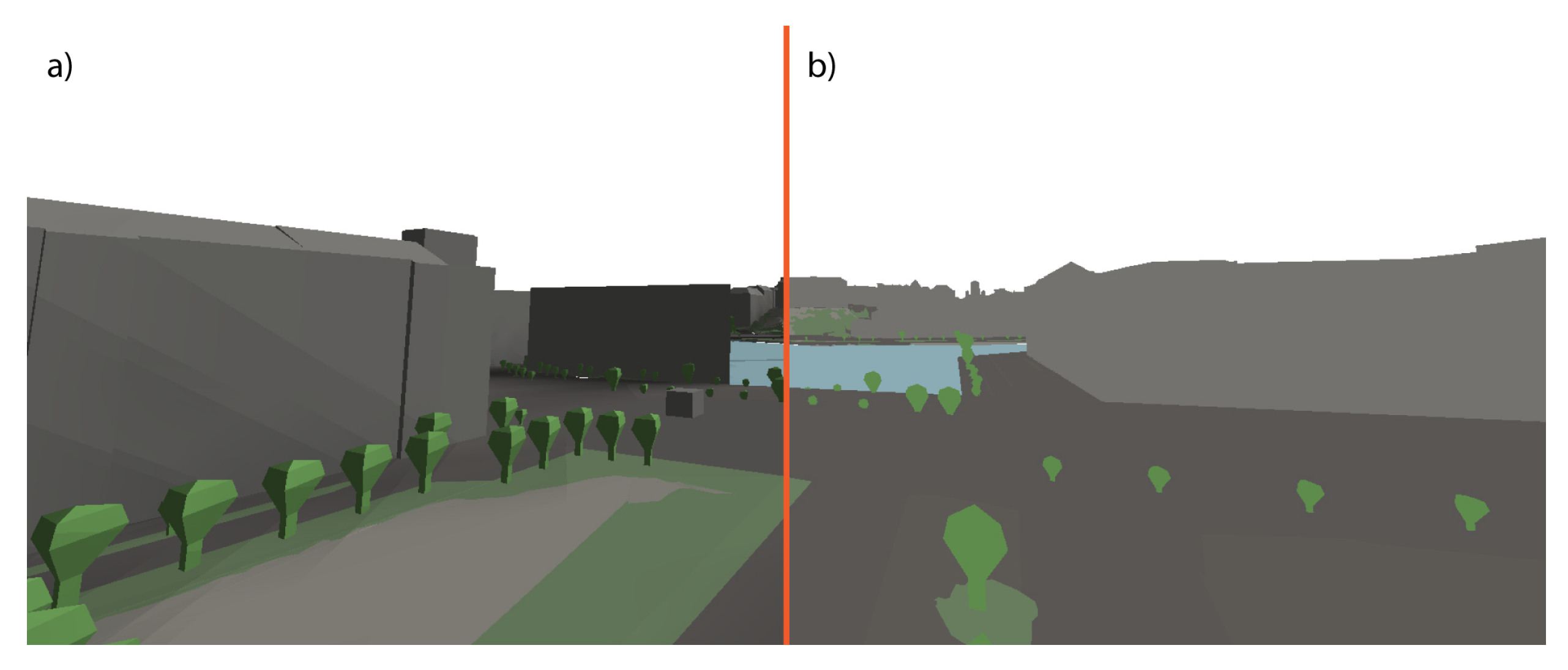
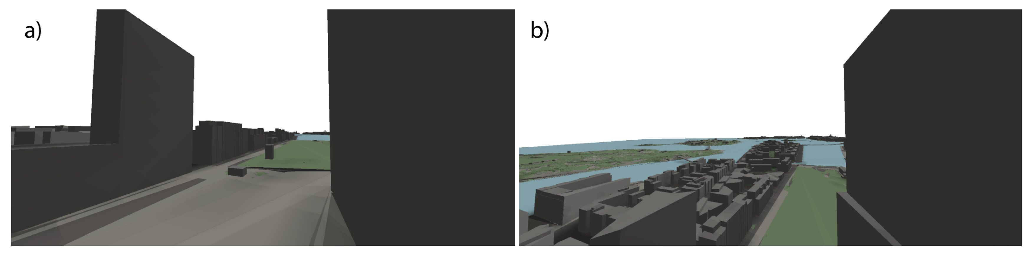
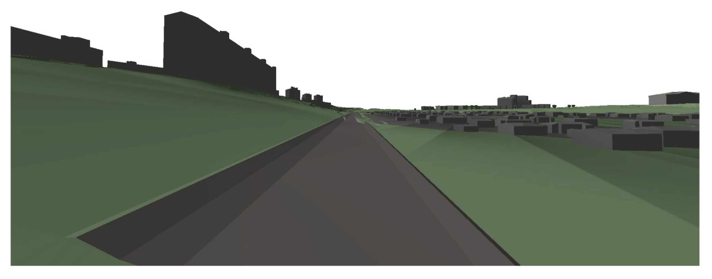
3.4. Semantic View Analysis in Browser

The semantic view analysis was realized with the pixel counting principle, extending a browser based CityJSON viewer [67], which in turn is based on a number of external libraries, namely the three.js JavaScript 3D library for rendering [68], Mapbox earcut library for polygon triangulation [69] and three.js orbit controls [70] for camera manipulation. The original viewer utility allows, in web browsers, the loading of a specified CityJSON model from a file, its visualization and query of individual objects’ attributes.
The analysis relies on the object division present in the CityJSON data. This object type information in encoded into object colors, after which the visibility of different city object types is determined with pixel counting from a rendered image. The results describe how a large fraction of the view is covered by each of the object types listed in Table 2. This approach has some similarities with the concepts of “object id layer” and “mask layer” shown in [13], effectively obtaining “masks” for objects belonging to each object type.
The viewer was modified to realize the semantic view analysis functionality, with the following most significant changes: (1) individual RGB colors were assigned to each of the 1st and 2nd level city objects (see Appendix A for colorization scheme), (2) the rendering and model illumination functionality were modified to allow for the production of pixel counting compatible image, (3) the pixel counting method (described in detail below) was implemented, and (4) the user interface was modified, including the results plotting function and a simplified keyboard based 1st person navigation for moving in a larger model. The running viewer is illustrated in Figure 3.
After the model is loaded and visualized, the user can initiate the semantic analysis of the current view. The analysis cycle consists of the following steps, interrupting the normal rendering loop of the viewer:
  • Interrupt conventional rendering loop;
  • Remove directional-, spot- and point lights, set ambient light to 100% intensity;
  • Render individual frame.
  • Obtain rendered frame as 2D array of pixel values
  • Compute pixel counts for semantic view analysis categories
  • Plot output (optional), log result to browser console (in CSV syntax)
  • Restore shadows & other light sources, set ambient light to original intensity
  • Render frame, display to user
  • Resume normal rendering loop
In practice, the analysis relies on obtaining a shadeless image from the rendering, accomplished by modifying the light sources. The obtained image is then utilized for pixel counting, relying on object specific predefined colors. Figure 4a illustrates the view displayed to the user from a street scene and the Figure 4b the unlit image used for pixel counting. The colorization applied for CityJSON objects is given in Table A1. In colorization, we aimed for color choices that would be suitable for visualization, but not having identical colors for any of the objects, thus allowing separation of different object types in analysis. The colors are hardcoded into the analysis tool, but can naturally be altered from the source code if required.

3.5. Experiments

Two sets of experiments were performed to evaluate the suitability of the semantic view analysis method to the use cases of view analysis in property evaluation (Section 3.5.1) and evaluation of the urban green infrastructure via the GVI (Section 3.5.2). Identical 3D city model and browser based analysis method were utilized in both experiments.

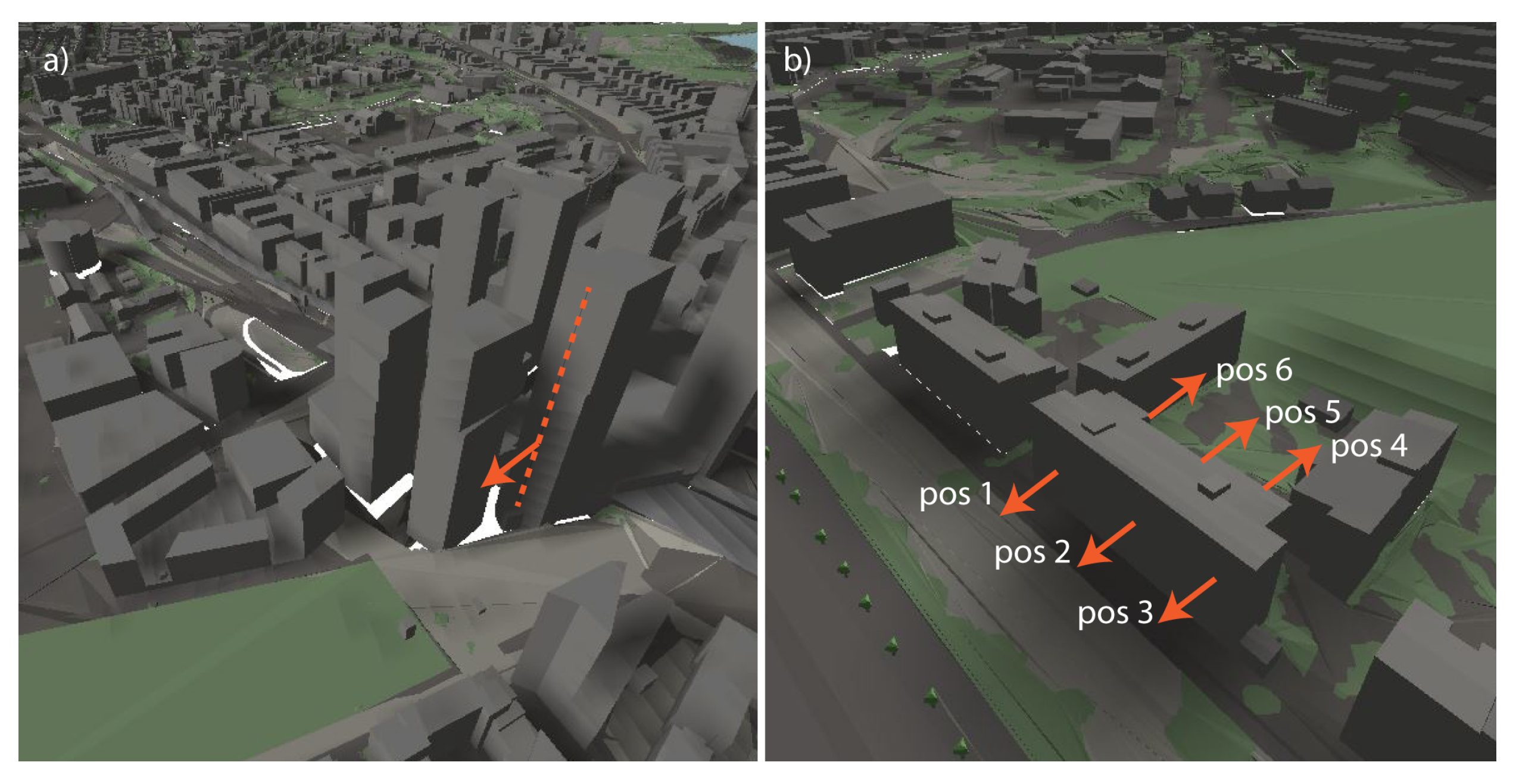
3.5.1. View Analysis for Varying Viewing Positions in Buildings

The semantic view analysis was tested on two simple example cases related to real estate valuation, mimicking the analysis of window-specific vistas as seen e.g., in [35]. In the first one (Figure 5a), the camera was positioned on the facade of a planned high-rise building, contained in the 3D city model. The analysis was repeated whilst increasing the height of the camera, effectively traversing the facade upwards and representing different apartment floor levels. In the second example (Figure 5b), the analysis was repeated from the same height, but looking outwards to different sides of a street side building.

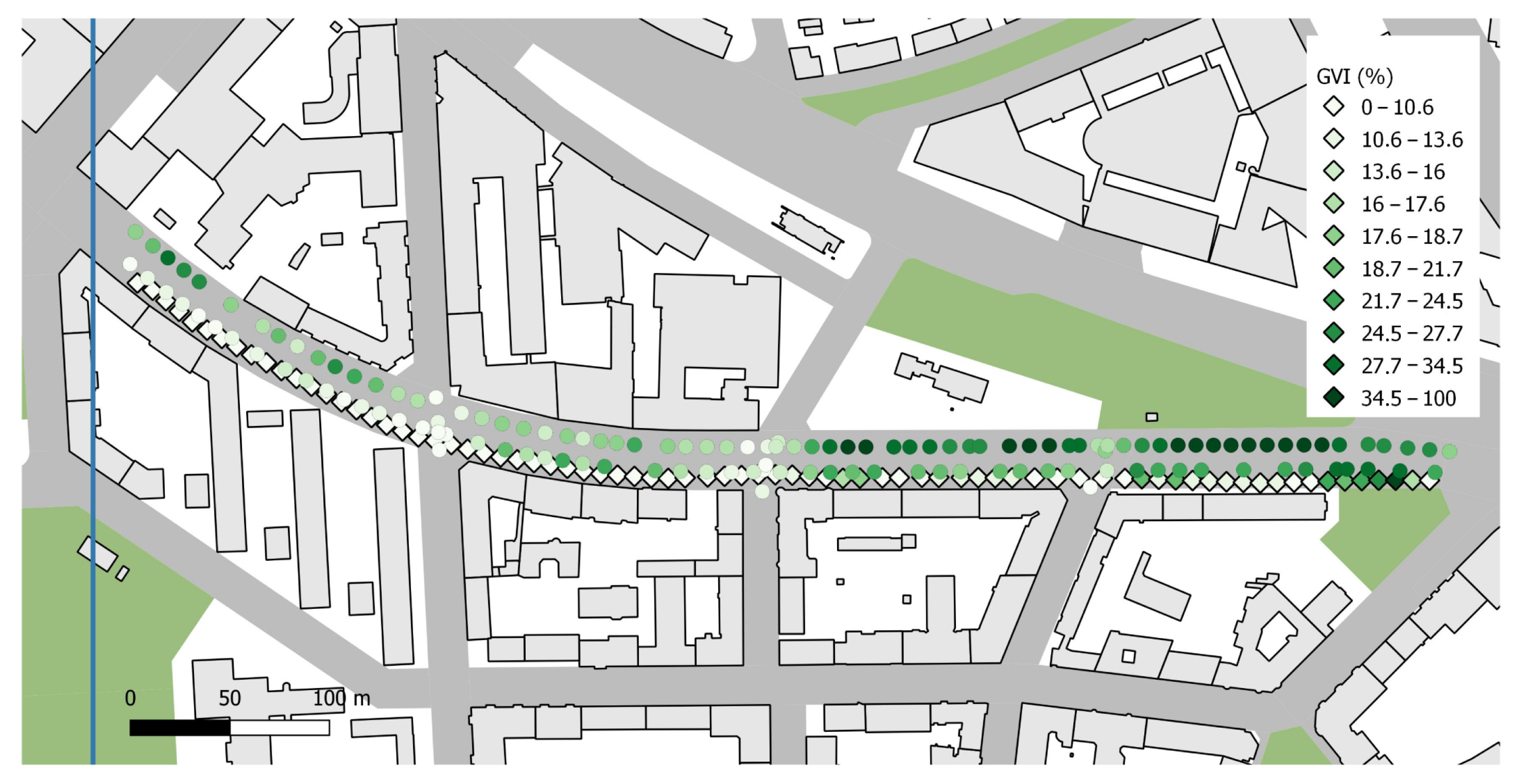
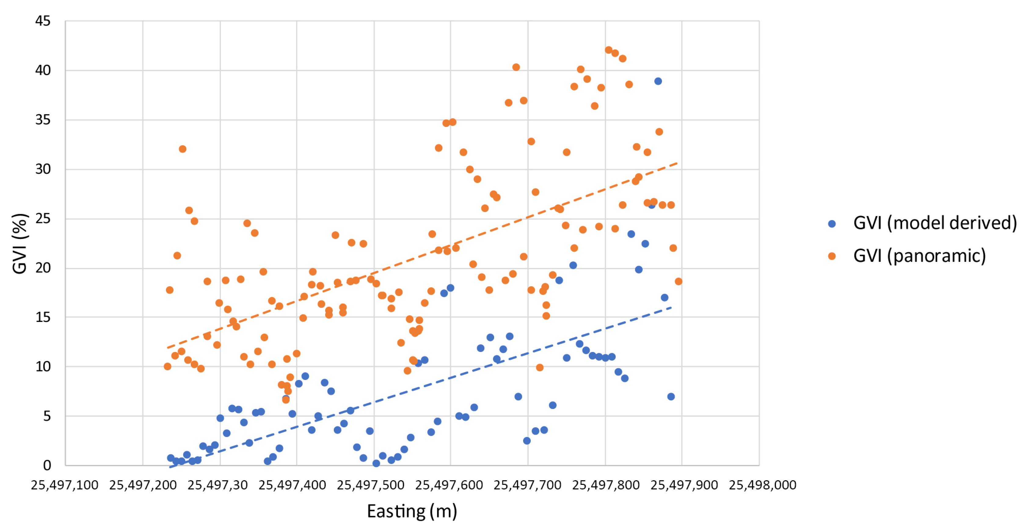
3.5.2. Comparison of Model Derived and Panoramic Image Street Level GVI

Following the concept of utilizing street level data for evaluation of urban greenery (as in e.g., [44]), the semantic view analysis was applied for estimating the amount of visible green elements in the 3D city model.
The semantic view analysis results were compared with the GVI obtained from Google Street View panoramic images, utilizing an open dataset from [30], using the panoramic GVI value computed for image acquisition locations. In total, the dataset consists of 92,126 points with the panoramic GVI being computed for each point as the mean of GVI’s for the six segments of the panoramic image [30]. The panoramic GVI in data varies between 0.01–86.29%.
For comparison, points from three street segments (test street 1–3) were separated from the data, with the first segment having a varying GVI along the segment, the second having a low GVI and the third segment having a mostly high GVI. The panoramic image acquisition dates for the segments varied between July 2009 and September 2011, whereas the CityGML model used for the building models had been published in 2019. Therefore, streets with no buildings completed after 2008 were chosen to minimize unnecessary discrepancies between the compared datasets. The test segments are shown on the map in Figure 6, while their key characteristics are given in Table 3.
The experiment was performed by firstly navigating the virtual camera to the approximate beginning of the street segment and then progressing along the street, running the semantic view analysis and logging the results on an even step. Test street 1 was progressed from west to east, test street 2 from north to south, and test street 3 from east to west. The camera height was controlled manually, aiming for a height similar to the Google Street View images used in the reference data set. From the results, a simple equivalent of GVI was computed with the following Equation (1):
G V I E s t i m a t e = ( P l a n t C o v e r P i x e l s + S o l i t a r y V e g e t a t i o n O b j e c t P i x e l s ) / T o t a l P i x e l s
The analysis relies on the assumption that, out of the objects present in the 3D city model (Table 2), the objects belonging to plant cover and solitary vegetation objects represent the green elements in the model. The computation of the size of the fraction of the view is covered by these objects and therefore returns the amount of green present in the view. As the rendered image consists of a known total amount of pixels, the GVI is therefore estimated via computation of these pixels as a fraction of the total pixels, as in Equation (1).

4. Results

4.1. Data Integration in CityJSON

As a result of the data integration pipeline, a 3D city model combining the 3D building and bridge models with road and green area polygons, and land cover classification polygons with tree objects corresponding to the Helsinki tree register was produced in the CityJSON format. In total, the model consists of 36,555 objects and requires approx. 155 MB of disk space. Figure 7b shows the model visualized with the online CityJSON viewer, Ninja [71]. Further images of the model are provided along the results from experiments, in Figures 8, 10 and 12–14.

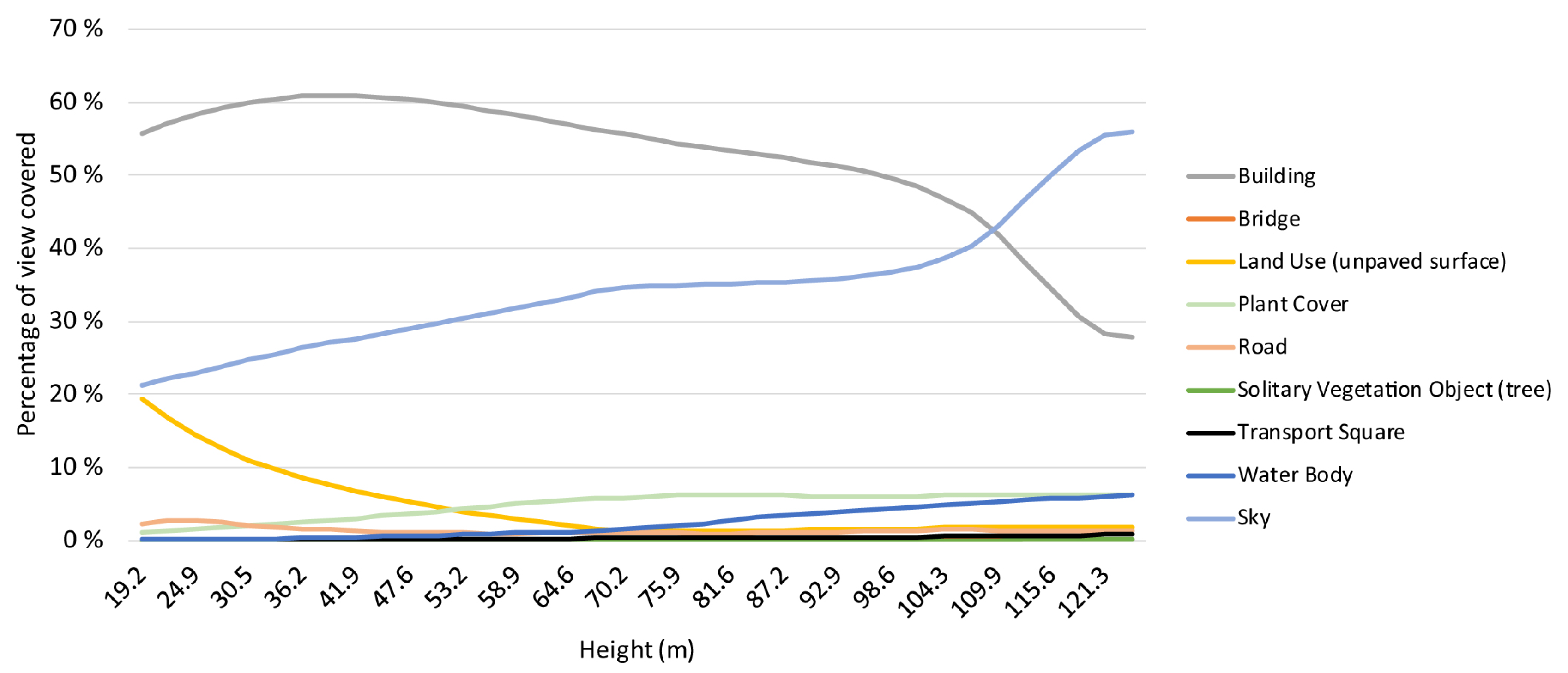
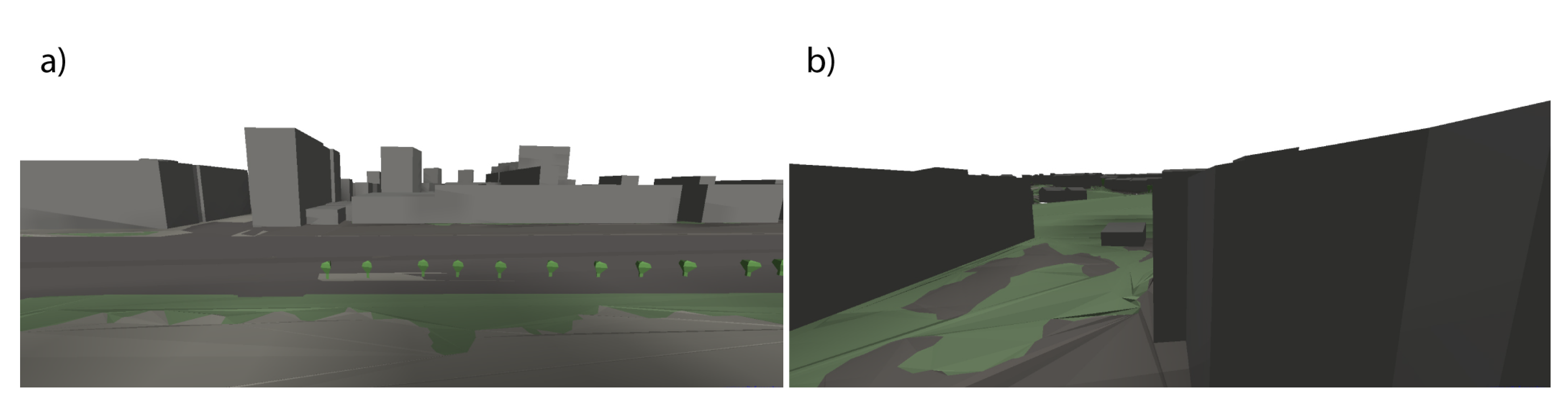
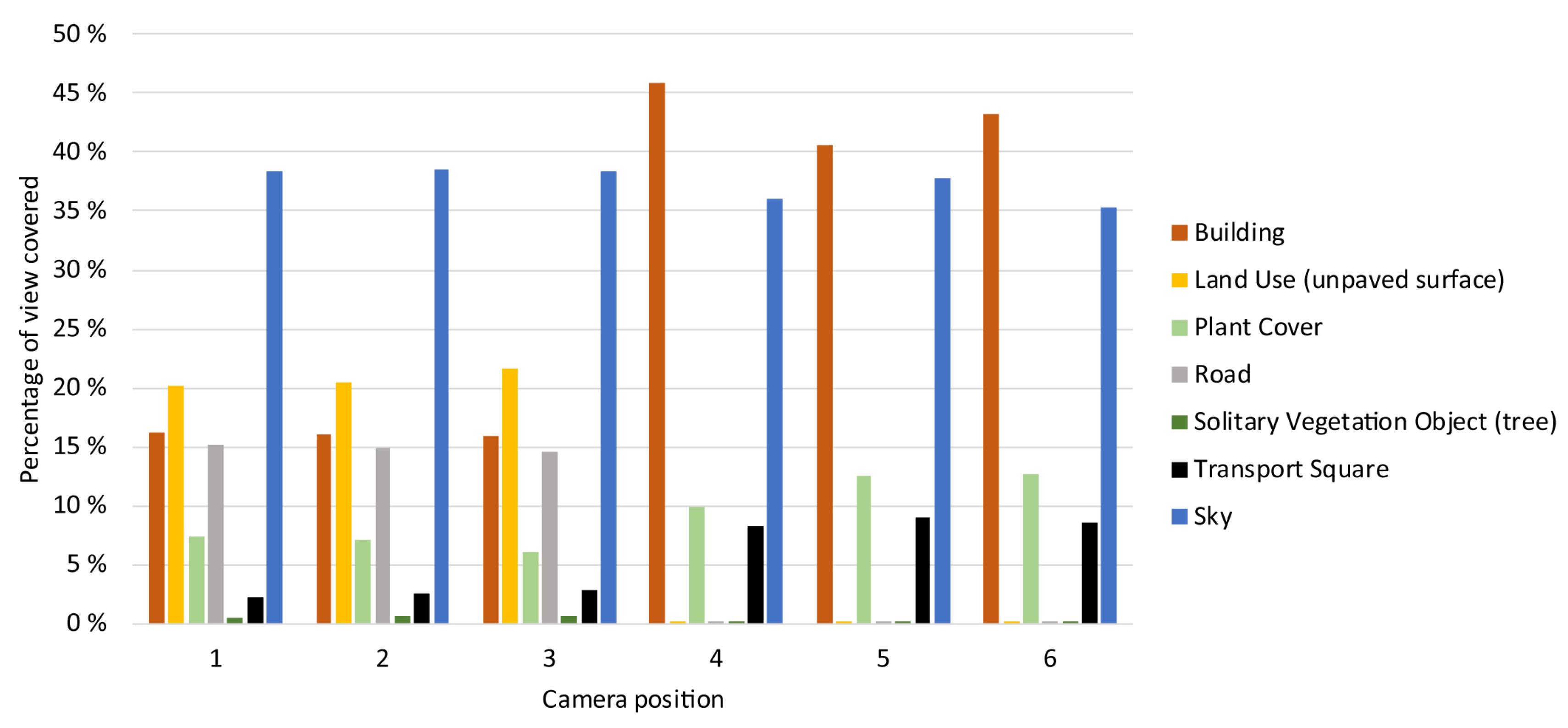
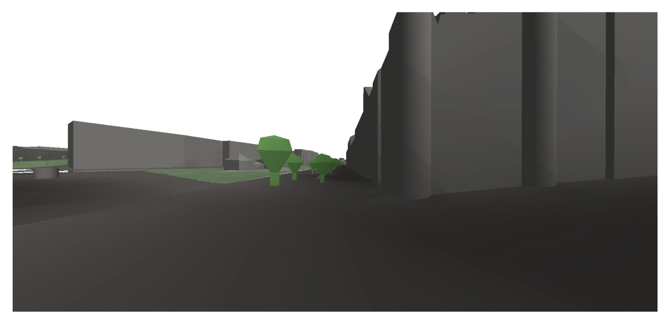
4.2. View Analysis for Varying Viewing Positions in Buildings

For the two small examples obtained from the experiment described in Section 3.5.1, the results are provided in Figure 8, Figure 9, Figure 10 and Figure 11.
When moving upwards in the building, the height naturally affects the vistas (Figure 8). Lower, the view is dominated by surrounding buildings and the land surface (Figure 8a). As the camera moves higher, a more open sky and sea view is gradually revealed (Figure 8b). More greenery also becomes visible. The sky-view increases dramatically after the camera surpasses the adjacent building (which is slightly lower), at approx. 110 m (Figure 9).
When alternating the viewing position in the building, Figure 10 shows the views from two viewing positions on opposite sides of the building. Even though there appears to be significantly more green areas visible from the side not facing the street (Figure 10b), a significant part of this is occluded by the nearby buildings (Figure 11).

4.3. Comparison of Model Derived and Panoramic Image Street Level GVI

A set of demonstration images used for the semantic view analysis from street segments, and onward for the GVI estimation, are shown in Figure 12, Figure 13 and Figure 14. The results for GVI (as computed according to Equation (1)) obtained from the semantic view analysis utilizing the CityJSON model combining multiple datasets are given in Table 4. For the street segment 1 containing (in reference data) a clearly varying GVI, the camera position specific obtained GVI values are illustrated in Figure 15, along with the panoramic imaging positions and their respective GVI values. In addition, a comparison plot of image specific GVI values, arranged according to the easting coordinate, is provided in Figure 16. As the general direction of the street is from west to east, the easting coordinate of the camera position is enough to describe the progression along the street.

5. Discussion

Utilizing the presented analysis method and the model produced with the data integration pipeline, the semantic view analysis was successfully applied in the presented experiments. The results describe the elements visible from a given location, and can also be applied to object type specific analysis, such as GVI estimation. The apparent main benefits of the model derived semantic view analysis are the freedom of choosing the point-of-view, and independence from e.g., seasonal variations or lighting conditions, both of which are difficult to attain with photographic data sets. In addition, the analysis can be performed relying on current 3D city models and GIS data, without additional measuring work. Finally, as the analysis is based on the model, it can easily be applied with planned objects as well, if they are integrated into the 3D city model.
The potential issues of the proposed method include its sensitivity to small variations of the camera position when there are objects very close to the camera. This can be observed in Figure 8b and Figure 10b, where the neighboring building covers a large portion of the view. A small translation or rotation of the camera can in this situation significantly affect the results. The same phenomena can potentially be seen in the variations of the estimated GVI between adjacent camera positions in Figure 16. As the virtual camera moves past a tree object, the GVI momentarily becomes quite large, before dropping again when the tree is outside the camera view. In a similar manner, the properties of the virtual camera, such as its field of view, will affect the results. However, the same issues are present when performing view analysis from real images as well.

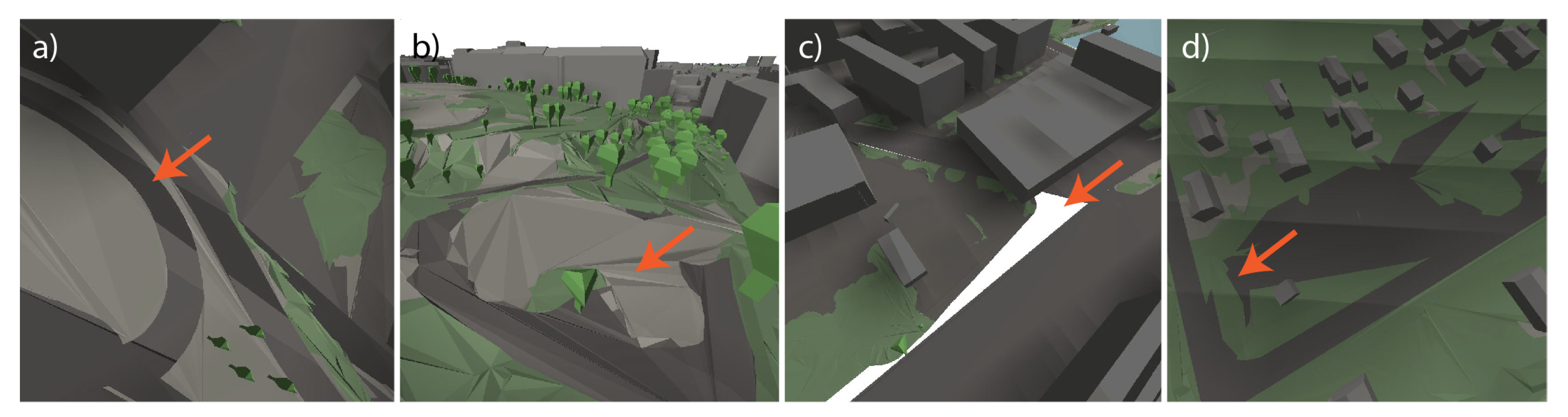
5.1. Notes on the Applied Data Integration Process

While the applied data integration process (described in Section 3.3) proved to be applicable for integrating various existing data sets to the CityGML model containing buildings and bridges, in CityJSON format, it still contains some apparent shortcomings, both concerning the model geometry and its conformance with the city modeling standards.
As the representation of terrain surface in the model was obtained by combining aerial imagery derived polygons and polygons from the city registers, the resulting surface contains a number of issues. In some cases, the data sets appear to contain differences likely originating from temporal changes (Figure 17a). As a separate DEM was used to obtain heights for the polygon points, the surface geometry also contains errors (Figure 17b). In addition, there are some gaps (Figure 17c) and erroneously overlapping objects (Figure 17d) present in the model. Many of these issues could be solved by processing the DEM to form a triangulated irregular network (TIN) for the terrain, and then using the desired polygon objects to clip this TIN into sub-segments. An alternative method would be to bring the land cover classification information to the system via a texture image on the terrain surface. In an optimal situation, the 3D city model, maintained by the city authorities, would contain a description of the terrain and the objects covering it.
The data integration results also had limitations concerning the data quality when looking from a city information modeling perspective. Firstly, the produced CityJSON files, while syntactically valid CityJSON files, do not meet the specification of CityGML standard concerning the attributes of the generated objects and their respective name spaces. Secondly, the first level city object “Land use” was in the selected case applied to describe a collection of non-developed, but non-vegetated land cover classes (bare bedrock, bare ground). This allows their separation in the semantic view estimation but is hardly the intended use for this object type.
Clearly, the development of a standard compliant data integration method for converting e.g., land cover classification polygons into 3D city model objects remains to be realized. However, the presented data integration pipeline did succeed in firstly obtaining the data required for realizing and demonstrating the semantic view analysis (which would have been rather fruitless with building and bridge models only, or at least produced results with more restricted application potential) and, secondly, in experimenting with the CityJSON format for data integration, and finding it rather easily applicable for the purpose. In this respect, the stated research aims were met.

5.2. On GVI Comparison with Panoramic Images

When looking at the results from GVI estimation performed via rendering synthetic views from the model and applying the semantic view analysis, it is clear that the results contain significant mismatches when compared with the panoramic image derived GVI applied as reference data. This is expected, as the reference data are produced as an average of six images (with unspecified vertical opening angle) together covering a horizontal angle of 360 degrees. In the model derived GVI, a single camera view having a horizontal fov of 90 degrees was utilized. Expecting matching results from two different imaging configurations would not be realistic.
In addition to the aforementioned difference in imaging geometry, there are several other potential explanations for errors encountered in the presented comparison: firstly, the imaging positions are not accurately matched either, which may give errors especially when moving close to large objects that may cover a large segment of the view. The differences in camera heights are also a potential source of error. Secondly, there are differences between the datasets, mainly arising from the issues of the CityJSON model and its source data. To offer a few examples: the tree register contains only the major roadside and park trees in the city environment. Therefore, several trees and other green elements are missing from the data, and, correspondingly, from the model. All known trees are represented by the same object, scaled according to the stem diameter information, which also likely results in mismatches between the model and reality, as e.g., tree species and tree height are missing. Likewise, the green area polygons only represent the public green areas, and are therefore unable to cover the green areas on private lots. These are covered by the land cover classification map objects relying on remote sensing data, but with a lower accuracy. Finally, the GVI is also influenced by shrubs, wines, small patches of lawn, potted outdoor plants, etc. that are not found in any of the datasets used for producing the model. Because of these missing components that would in real life contribute to the GVI, lower values obtained from the model based estimation are not surprising. This calls for elements of smaller scale urban green infrastructure [43], including minor green elements, to be gathered and included in the CityGML convertible data sets.
However, the results seem to correlate to some extent: for both the test and reference data, the highest average GVI was found from the street segment 3 (49.1% panoramic GVI vs. 29.1% model derived GVI). The same holds true for the lowest and varying GVI’s as well (in segment 2: 5.7% vs. 0.01% and in segment 1: 21.0% vs. 7.6%). In similar manner, the standard deviation in both datasets remains highest in the test segment having the most varying GVI. Furthermore, the way in which the GVI varies in this dataset (test street segment 1) along the street is reflected in both datasets (Figure 12). Clearly, the model derived GVI is able to reflect the real GVI obtained from panoramic images. This would indicate that the semantic view analysis as derived from a 3D city model correlates with real-life views, at least with respect to a single group of city elements, the greenery.

5.3. On Limitations of Browser Based Implementation

Even though the semantic view analysis was successfully implemented and applied, it is subject to a number of limitations stemming from its browser based realization. Firstly, as the viewer operates by loading the entire model to the memory, the size of the usable model is limited by the browser’s memory requirements. The tested model, obtained via data integration was likely at the upper performance limits of the system, requiring a total of 3.2 GB of RAM on a 64-bit Google Chrome web browser for processing and visualizing the total of 36,555 objects.
On a more general level, it can be said that the use of files for model transfer does not represent a state-of-the-art approach. In the current system, the model bounds may influence the results, as objects beyond the model bounds can potentially still be visible to a given point in a model in reality. A more feasible implementation for professional use should most likely utilize a relational database for model storage and interfaces supporting tiled retrieval and incremental level of detail for rendering (see, e.g., [72]).
As the analysis is realized by pixel counting from a rendered image, its resolution is dependent on the aspect ratio and display resolution of the system used. For the system utilized in the presented experiment, the laptop screen with a typical display resolution of 1920 by 1080 pixels resulted (excluding the browser toolbars, etc.) in an analysis image of 1920 by 937 pixels, resulting in a total number of 1,799,040 pixels. This is a subject to browsers settings, screen resolution, and the screen magnification ratio (that, on a Windows platforms, can be used to separate rendering resolution from the pixel resolution of the display). The screen resolution also determines a minimum fraction that can be distinguished with the pixel counting analysis used. For the resolution of 1920 by 937 pixels, the smallest possible increment is a single pixel, in this case, a 1/1,799,040th part of the total view.

5.4. Future Research Topics

Summarizing the mentioned discussion topics, several promising research and development directions can be identified. Concerning the CityJSON data integration pipeline, further development allowing the production of CityGML compliant models from similar data sources is an apparent development task. In the presented case, the compliance was not actively targeted, and some of the object classes were misused to support the analysis being implemented.
For the semantic view analysis, validating the results against datasets covering other factors (e.g., unobstructed sky-view or view to the sea) could potentially be accomplished via automated analysis of panoramic images, or alternatively via comparison with more photorealistic datasets, such as the Helsinki mesh model [3]. The analysis could also be implemented as panoramic, borrowing, for example, the approach used in [30] to compute the panoramic GVI. It is also possible to try further refine the semantic understanding offered by the analysis by separating e.g., distant and close by objects. Comparing the results against the human experience [48] would also offer a significant research opportunity, potentially realized e.g., via walking interviews.
Additional technical possibilities are offered by the virtual reality (VR) systems, and the emerging WebXR systems allowing their utilization in browser based applications. The view analysis could be integrated with VR visualization and, performance permitting, used in real time to obtain a better understanding of the virtual experience. Another possibility is the utilization of classified point clouds as source data (see, e.g., [73]). Dense, terrestrial point clouds, if classified and visualized via a suitable system, could offer a much more detailed depiction of the urban environment than current semantic 3D city models. With game engine technology, even the combination of point cloud data and VR visualization could be attained [74].
Further integration of the 3D city model derived semantic view analysis with its potential applications, such as green infrastructure evaluation or real estate valuation would be beneficial and could support the uptake of the proposed method. Thus, the benefits of view analyses offering a human-scale approach [41,48,49,52,57] to the quality of urban green environment [43] and dwellings [25,28,32,33], could be achieved. In practice, this could be realized via the integration of the analysis tool with the existing 3D city model application development platforms, such as CesiumJS [75]. This way, the view analysis could become a complementary tool for processes that currently leverage the 3D city models on these platforms, such as participatory urban planning [76,77]. Finally, as the open data sets get richer, e.g., in terms of 3D green infrastructure data [78], the CityGML based urban view analyses could be utilized up to their full potential.

6. Conclusions

The integration of view analysis with a semantic 3D city model appears to offer the benefits of allowing (1) the analysis of views with respect to different types of urban elements contained in the model, (2) the use of model derived, synthetic views, thus making it possible to run the analysis from arbitrary positions, and (3) the use of view analysis in planning processes utilizing the 3D city model for scenario analysis.
In a situation where the existing 3D city model is, in terms of objects contained, not semantically rich enough to support this analysis, 2D GIS datasets can be used to enrich the model and make it more useful in this respect. Here, the CityJSON format was found beneficial, via the simplicity of writing it in the Python programming language. Further development would be required to turn this data integration pipeline into a more generic tool for enriching the existing 3D city models with additional objects.
The semantic view analysis was implemented as a browser based application, relying on the existing CityJSON viewer. It allows free camera manipulation and the near-real time analysis of the current view. Two sets of experiments were performed, firstly obtaining a set of view analysis data mimicking the real estate valuation and infill development use cases and, secondly, comparing the results to panoramic image derived GVI. The analysis tool was found successful in obtaining and analyzing vistas from different positions of buildings. In the comparison with panoramic image GVI, the results roughly correlated, but the obtained GVI values were significantly lower. This is likely due to the different camera viewing angle and the discrepancy between the 3D city model and the real environment, especially with the smaller green elements that are missing from the model. Several promising development directions can be identified based on the current implementation and experiment results, including the integration of the semantic view analysis with (a) VR visualization and (b) city model application development platforms. The comparison of results with the perceived pedestrian experience also remains a vital research topic.

Author Contributions

Conceptualization: Juho-Pekka Virtanen; Kaisa Jaalama; Tuulia Puustinen; Arttu Julin; Hannu Hyyppä; Juha Hyyppä; Methodology: Juho-Pekka Virtanen; Kaisa Jaalama; Writing—original draft: Juho-Pekka Virtanen; Kaisa Jaalama; Tuulia Puustinen; Arttu Julin; Hannu Hyyppä; Software: Juho-Pekka Virtanen; Formal analysis: Juho-Pekka Virtanen; Kaisa Jaalama; Funding acquisition: Juho-Pekka Virtanen; Kaisa Jaalama; Tuulia Puustinen; Arttu Julin; Juha Hyyppä; Hannu Hyyppä. All authors have read and agreed to the published version of the manuscript.

Funding

This research project was supported by the Academy of Finland, the Center of Excellence in Laser Scanning Research (CoE-LaSR) (No. 272195, 307362) and the Strategic Research Council projects, “Competence-Based Growth Through Integrated Disruptive Technologies of 3D Digitalization, Robotics, Geospatial Information and Image Processing/Computing—Point Cloud Ecosystem” (No. 293389, 314312) and “Smartland” (No. 327800), the European Social Fund (S21997) and the City of Helsinki Innovation fund.

Institutional Review Board Statement

Not applicable.

Informed Consent Statement

Not applicable.

Data Availability Statement

The utilized test data sets are freely available from sources listed in Table 1. The model depicted in Section 4.1 in available at: http://0-doi-org.brum.beds.ac.uk/10.5281/zenodo.4576627 (accessed on 3 January 2021), the source code for self-developed data integration tools Section 3.3 at https://0-doi-org.brum.beds.ac.uk/10.5281/zenodo.4576585 (accessed on 3 January 2021) and the source code for the browser based analysis tool Section 3.4 at https://0-doi-org.brum.beds.ac.uk/10.5281/zenodo.4576591 (accessed on 3 January 2021).

Acknowledgments

The authors are grateful for the City of Helsinki 3D+ team for support with open data sets, and for Markus Sarlin for helping out with LaTeX.

Conflicts of Interest

The authors declare no conflict of interest.

Abbreviations

The following abbreviations are used in this manuscript:
VRVirtual reality
UGIUrban green infrastructure
GVIGreen view index
NDVINormalized difference vegetation index
JSONJavaScript object notation
GSVGoogle street view

Appendix A

Table A1. The coloring scheme applied in rendering for the semantic view analysis.
1st or 2nd Level City ObjectR, G, B Values (8 Bit)Color Sample
Building115, 114, 111
Building part143, 139, 126
Building installation97, 94, 84
Bridge117, 117, 117
Bridge part74, 74, 74
Bridge installation105, 105, 105
Bridge construction element122, 122, 122
City object group90, 95, 97
City furniture123, 130, 133
Generic city object165, 173, 176
LandUse133, 131, 123
Plant cover104, 125, 94
Railway89, 75, 63
Road89, 86, 84
Solitary vegetation object94, 140, 76
TINRelief122, 135, 116
Transport square92, 89, 85
Tunnel69, 67, 64
Tunnel part102, 99, 95
Tunnel installation107, 101, 92
Water body139, 172, 181

References

  1. Zhu, Q.; Hu, M.; Zhang, Y.; Du, Z. Research and practice in three-dimensional city modeling. Geo-Spat. Inf. Sci. 2009, 12, 18–24. [Google Scholar] [CrossRef]
  2. Gröger, G.; Plümer, L. CityGML—Interoperable semantic 3D city models. ISPRS J. Photogramm. Remote Sens. 2012, 71, 12–33. [Google Scholar] [CrossRef]
  3. Cousins, S. 3D mapping Helsinki: How mega digital models can help city planners. Constr. Res. Innov. 2017, 8, 102–106. [Google Scholar] [CrossRef]
  4. Biljecki, F.; Stoter, J.; Ledoux, H.; Zlatanova, S.; Çöltekin, A. Applications of 3D City Models: State of the Art Review. ISPRS Int. J. Geo-Inf. 2015, 4, 2842–2889. [Google Scholar] [CrossRef] [Green Version]
  5. Bao, K.; Padsala, R.; Thrän, D.; Schröter, B. Urban Water Demand Simulation in Residential and Non-Residential Buildings Based on a CityGML Data Model. ISPRS Int. J. Geo-Inf. 2020, 9, 642. [Google Scholar] [CrossRef]
  6. HosseiniHaghighi, S.; Izadi, F.; Padsala, R.; Eicker, U. Using Climate-Sensitive 3D City Modeling to Analyze Outdoor Thermal Comfort in Urban Areas. ISPRS Int. J. Geo-Inf. 2020, 9, 688. [Google Scholar] [CrossRef]
  7. Agugiaro, G.; González, F.G.G.; Cavallo, R. The City of Tomorrow from… the Data of Today. ISPRS Int. J. Geo-Inf. 2020, 9, 554. [Google Scholar] [CrossRef]
  8. Yao, Z.; Nagel, C.; Kunde, F.; Hudra, G.; Willkomm, P.; Donaubauer, A.; Adolphi, T.; Kolbe, T.H. 3DCityDB—A 3D geodatabase solution for the management, analysis, and visualization of semantic 3D city models based on CityGML. Open Geospat. Data Softw. Stand. 2018, 3, 5. [Google Scholar] [CrossRef] [Green Version]
  9. Döllner, J.; Kolbe, T.H.; Liecke, F.; Sgouros, T.; Teichmann, K. The virtual 3d city model of berlin-managing, integrating, and communicating complex urban information. In Proceedings of the 25th International Symposium on Urban Data Management (UDMS), Aalborg, Denmark, 15–17 May 2006. [Google Scholar]
  10. Czyńska, K. Application of Lidar Data and 3D-City Models in Visual Impact Simulations of Tall Buildings. ISPRS Int. Arch. Photogramm. Remote Sens. Spat. Inf. Sci. 2015, XL-7/W3, 1359–1366. [Google Scholar] [CrossRef] [Green Version]
  11. Wu, H.; He, Z.; Gong, J. A virtual globe-based 3D visualization and interactive framework for public participation in urban planning processes. Comput. Environ. Urban Syst. 2010, 34, 291–298. [Google Scholar] [CrossRef]
  12. Hildebrandt, D.; Döllner, J. Service-oriented, standards-based 3D geovisualization: Potential and challenges. Comput. Environ. Urban Syst. 2010, 34, 484–495. [Google Scholar] [CrossRef]
  13. Hagedorn, B.; Hildebrandt, D.; Döllner, J. Towards Advanced and Interactive Web Perspective View Services. In Developments in 3D Geo-Information Sciences; Neutens, T., Maeyer, P., Eds.; Springer: Berlin/Heidelberg, Germany, 2010; pp. 33–51. [Google Scholar] [CrossRef] [Green Version]
  14. Virtanen, J.P.; Hyyppä, H.; Kurkela, M.; Vaaja, M.T.; Puustinen, T.; Jaalama, K.; Julin, A.; Pouke, M.; Kukko, A.; Turppa, T.; et al. Browser based 3D for the built environment. Nord. J. Surv. Real Estate Res. 2018, 13, 54–76. [Google Scholar] [CrossRef]
  15. Romero Rodríguez, L.; Duminil, E.; Sánchez Ramos, J.; Eicker, U. Assessment of the photovoltaic potential at urban level based on 3D city models: A case study and new methodological approach. Sol. Energy 2017, 146, 264–275. [Google Scholar] [CrossRef]
  16. Julin, A.; Jaalama, K.; Virtanen, J.P.; Maksimainen, M.; Kurkela, M.; Hyyppä, J.; Hyyppä, H. Automated Multi-Sensor 3D Reconstruction for the Web. ISPRS Int. J. Geo-Inf. 2019, 8, 221. [Google Scholar] [CrossRef] [Green Version]
  17. Virtanen, J.P.; Kurkela, M.; Turppa, T.; Vaaja, M.T.; Julin, A.; Kukko, A.; Hyyppä, J.; Ahlavuo, M.; von Numers, J.; Haggrén, H.; et al. Depth camera indoor mapping for 3D virtual radio play. Photogramm. Rec. 2018, 33, 171–195. [Google Scholar] [CrossRef] [Green Version]
  18. Julin, A.; Jaalama, K.; Virtanen, J.P.; Pouke, M.; Ylipulli, J.; Vaaja, M.; Hyyppä, J.; Hyyppä, H. Characterizing 3D City Modeling Projects: Towards a Harmonized Interoperable System. ISPRS Int. J. Geo-Inf. 2018, 7, 55. [Google Scholar] [CrossRef] [Green Version]
  19. Ledoux, H.; Arroyo Ohori, K.; Kumar, K.; Dukai, B.; Labetski, A.; Vitalis, S. CityJSON: A compact and easy-to-use encoding of the CityGML data model. Open Geospat. Data Softw. Stand. 2019, 4, 4. [Google Scholar] [CrossRef]
  20. Nys, G.A.; Poux, F.; Billen, R. CityJSON Building Generation from Airborne LiDAR 3D Point Clouds. ISPRS Int. J. Geo-Inf. 2020, 9, 521. [Google Scholar] [CrossRef]
  21. Vitalis, S.; Arroyo Ohori, K.; Stoter, J. CityJSON in QGIS: Development of an open-source plugin. Trans. GIS 2020, 24, 1147–1164. [Google Scholar] [CrossRef]
  22. Kumar, K.; Ledoux, H.; Stoter, J. Dynamic 3D Visualization of Floods: Case of the Netherlands. ISPRS Int. Arch. Photogramm. Remote Sens. Spat. Inf. Sci. 2018, XLII-4/W10, 83–87. [Google Scholar] [CrossRef] [Green Version]
  23. Delikostidis, I.; Engel, J.; Retsios, B.; van Elzakker, C.P.; Kraak, M.J.; Döllner, J. Increasing the Usability of Pedestrian Navigation Interfaces by means of Landmark Visibility Analysis. J. Navig. 2013, 66, 523–537. [Google Scholar] [CrossRef] [Green Version]
  24. Yang, P.P.J.; Putra, S.Y.; Li, W. Viewsphere: A GIS-Based 3D Visibility Analysis for Urban Design Evaluation. Environ. Plan. B Plan. Des. 2007, 34, 971–992. [Google Scholar] [CrossRef] [Green Version]
  25. Yu, S.; Yu, B.; Song, W.; Wu, B.; Zhou, J.; Huang, Y.; Wu, J.; Zhao, F.; Mao, W. View-based greenery: A three-dimensional assessment of city buildings’ green visibility using Floor Green View Index. Landsc. Urban Plan. 2016, 152, 13–26. [Google Scholar] [CrossRef]
  26. Yu, S.M.; Han, S.S.; Chai, C.H. Modeling the Value of View in High-Rise Apartments: A 3D GIS Approach. Environ. Plan. B Plan. Des. 2007, 34, 139–153. [Google Scholar] [CrossRef]
  27. Hamilton, S.E.; Morgan, A. Integrating lidar, GIS and hedonic price modeling to measure amenity values in urban beach residential property markets. Comput. Environ. Urban Syst. 2010, 34, 133–141. [Google Scholar] [CrossRef] [Green Version]
  28. Li, X.; Zhang, C.; Li, W.; Ricard, R.; Meng, Q.; Zhang, W. Assessing street-level urban greenery using Google Street View and a modified green view index. Urban For. Urban Green. 2015, 14, 675–685. [Google Scholar] [CrossRef]
  29. Bishop, I.D. Assessment of Visual Qualities, Impacts, and Behaviours, in the Landscape, by Using Measures of Visibility. Environ. Plan. B Plan. Des. 2003, 30, 677–688. [Google Scholar] [CrossRef]
  30. Toikka, A.; Willberg, E.; Mäkinen, V.; Toivonen, T.; Oksanen, J. The green view dataset for the capital of Finland, Helsinki. Data Brief 2020, 30, 105601. [Google Scholar] [CrossRef]
  31. Gong, Z.; Ma, Q.; Kan, C.; Qi, Q. Classifying Street Spaces with Street View Images for a Spatial Indicator of Urban Functions. Sustainability 2019, 11, 6424. [Google Scholar] [CrossRef] [Green Version]
  32. Ye, Y.; Richards, D.; Lu, Y.; Song, X.; Zhuang, Y.; Zeng, W.; Zhong, T. Measuring daily accessed street greenery: A human-scale approach for informing better urban planning practices. Landsc. Urban Plan. 2019, 191, 103434. [Google Scholar] [CrossRef]
  33. Zhang, Y.; Dong, R. Impacts of Street-Visible Greenery on Housing Prices: Evidence from a Hedonic Price Model and a Massive Street View Image Dataset in Beijing. ISPRS Int. J. Geo-Inf. 2018, 7, 104. [Google Scholar] [CrossRef] [Green Version]
  34. Chen, J.; Zhou, C.; Li, F. Quantifying the green view indicator for assessing urban greening quality: An analysis based on Internet-crawling street view data. Ecol. Indic. 2020, 113, 106192. [Google Scholar] [CrossRef]
  35. Virtanen, J.P.; Puustinen, T.; Pennanen, K.; Vaaja, M.T.; Kurkela, M.; Viitanen, K.; Hyyppä, H.; Röonnholm, P. Customized visualizations of urban infill development scenarios for local stakeholders. J. Build. Constr. Plan. Res. 2015, 3, 68. [Google Scholar] [CrossRef] [Green Version]
  36. Czyńska, K. High Precision Visibility and Dominance Analysis of Tall Building in Cityscape On a basis of Digital Surface Model. In Proceedings of the 36th Annual Conference eCAADe 2018, Lodz, Poland, 17–21 September 2018. [Google Scholar]
  37. Puustinen, T.; Pennanen, K.; Falkenbach, H.; Viitanen, K. The distribution of perceived advantages and disadvantages of infill development among owners of a commonhold and its’ implications. Land Use Policy 2018, 75, 303–313. [Google Scholar] [CrossRef] [Green Version]
  38. Puustinen, T. Infill Development in Growing Urban Areas: Experiences in Finnish Housing Companies and Perspectives of Owner-Occupiers [Täydennysrakentaminen Kasvavilla Kaupunkialueilla: Kokemuksia Suomalaisissa Asunto-Osakeyhtiöissä ja Asukasosakkaiden Näkökulmia]. Ph.D. Thesis, Aalto University, Espoo, Finland, 2020. [Google Scholar]
  39. Ulrich, R. View through a window may influence recovery from surgery. Science 1984, 224, 420–421. [Google Scholar] [CrossRef] [Green Version]
  40. Tsunetsugu, Y.; Lee, J.; Park, B.J.; Tyrväinen, L.; Kagawa, T.; Miyazaki, Y. Physiological and psychological effects of viewing urban forest landscapes assessed by multiple measurements. Landsc. Urban Plan. 2013, 113, 90–93. [Google Scholar] [CrossRef]
  41. Helbich, M.; Yao, Y.; Liu, Y.; Zhang, J.; Liu, P.; Wang, R. Using deep learning to examine street view green and blue spaces and their associations with geriatric depression in Beijing, China. Environ. Int. 2019, 126, 107–117. [Google Scholar] [CrossRef]
  42. Li, X.; Ghosh, D. Associations between Body Mass Index and Urban “Green” Streetscape in Cleveland, Ohio, USA. Int. J. Environ. Res. Public Health 2018, 15, 2186. [Google Scholar] [CrossRef] [Green Version]
  43. Wolch, J.R.; Byrne, J.; Newell, J.P. Urban green space, public health, and environmental justice: The challenge of making cities ‘just green enough’. Landsc. Urban Plan. 2014, 125, 234–244. [Google Scholar] [CrossRef] [Green Version]
  44. Yang, J.; Zhao, L.; Mcbride, J.; Gong, P. Can you see green? Assessing the visibility of urban forests in cities. Landsc. Urban Plan. 2009, 91, 97–104. [Google Scholar] [CrossRef]
  45. Verma, D.; Jana, A.; Ramamritham, K. Machine-based understanding of manually collected visual and auditory datasets for urban perception studies. Landsc. Urban Plan. 2019, 190, 103604. [Google Scholar] [CrossRef]
  46. Wang, R.; Lu, Y.; Wu, X.; Liu, Y.; Yao, Y. Relationship between eye-level greenness and cycling frequency around metro stations in Shenzhen, China: A big data approach. Sustain. Cities Soc. 2020, 59, 102201. [Google Scholar] [CrossRef]
  47. Fu, Y.; Song, Y. Evaluating Street View Cognition of Visible Green Space in Fangcheng District of Shenyang with the Green View Index. In Proceedings of the 2020 Chinese Control and Decision Conference (CCDC), Hefei, China, 22–24 August 2020; pp. 144–148. [Google Scholar] [CrossRef]
  48. Falfán, I.; Muñoz-Robles, C.A.; Bonilla-Moheno, M.; MacGregor-Fors, I. Can you really see ‘green’? Assessing physical and self-reported measurements of urban greenery. Urban For. Urban Green. 2018, 36, 13–21. [Google Scholar] [CrossRef]
  49. Villeneuve, P.J.; Ysseldyk, R.L.; Root, A.; Ambrose, S.; DiMuzio, J.; Kumar, N.; Shehata, M.; Xi, M.; Seed, E.; Li, X.; et al. Comparing the Normalized Difference Vegetation Index with the Google Street View Measure of Vegetation to Assess Associations between Greenness, Walkability, Recreational Physical Activity, and Health in Ottawa, Canada. Int. J. Environ. Res. Public Health 2018, 15, 1719. [Google Scholar] [CrossRef] [Green Version]
  50. Ki, D.; Lee, S. Analyzing the effects of Green View Index of neighborhood streets on walking time using Google Street View and deep learning. Landsc. Urban Plan. 2021, 205, 103920. [Google Scholar] [CrossRef]
  51. Shen, Q.; Zeng, W.; Ye, Y.; Arisona, S.M.; Schubiger, S.; Burkhard, R.; Qu, H. StreetVizor: Visual Exploration of Human-Scale Urban Forms Based on Street Views. IEEE Trans. Vis. Comput. Graph. 2018, 24, 1004–1013. [Google Scholar] [CrossRef]
  52. Larkin, A.; Hystad, P. Evaluating street view exposure measures of visible green space for health research. J. Expo. Sci. Environ. Epidemiol. 2019, 29, 447–456. [Google Scholar] [CrossRef]
  53. Li, X. Examining the spatial distribution and temporal change of the green view index in New York City using Google Street View images and deep learning. Environ. Plan. Urban Anal. City Sci. 2020. [Google Scholar] [CrossRef]
  54. Zhou, H.; He, S.; Cai, Y.; Wang, M.; Su, S. Social inequalities in neighborhood visual walkability: Using street view imagery and deep learning technologies to facilitate healthy city planning. Sustain. Cities Soc. 2019, 50, 101605. [Google Scholar] [CrossRef]
  55. Yu, X.; Zhao, G.; Chang, C.; Yuan, X.; Heng, F. BGVI: A New Index to Estimate Street-Side Greenery Using Baidu Street View Image. Forests 2019, 10, 3. [Google Scholar] [CrossRef] [Green Version]
  56. DeFries, R.S.; Townshend, J.R.G. NDVI-derived land cover classifications at a global scale. Int. J. Remote Sens. 1994, 15, 3567–3586. [Google Scholar] [CrossRef]
  57. Kumakoshi, Y.; Chan, S.Y.; Koizumi, H.; Li, X.; Yoshimura, Y. Standardized Green View Index and Quantification of Different Metrics of Urban Green Vegetation. Sustainability 2020, 12, 7434. [Google Scholar] [CrossRef]
  58. 3D Models of Helsinki-Kalasatama Digital Twins Pilot Project’s CityGML Files. Available online: https://hri.fi/data/en_GB/dataset/helsingin-3d-kaupunkimalli/resource/cd7ed6e8-fd77-4319-bc67-692f7dfc43de (accessed on 5 February 2021).
  59. Register of Public Areas in the City of Helsinki. Available online: https://hri.fi/data/en_GB/dataset/helsingin-kaupungin-yleisten-alueiden-rekisteri (accessed on 5 February 2021).
  60. Metropolitan Area Land Cover. Available online: https://hri.fi/data/en_GB/dataset/paakaupunkiseudun-maanpeiteaineisto (accessed on 5 February 2021).
  61. Urban Tree Database of the City of Helsinki. Available online: https://hri.fi/data/en_GB/dataset/helsingin-kaupungin-puurekisteri (accessed on 5 February 2021).
  62. Elevation Model 2 m. Available online: https://www.maanmittauslaitos.fi/en/maps-and-spatial-data/expert-users/product-descriptions/elevation-model-2-m (accessed on 5 February 2021).
  63. citygml-Tools. Available online: https://github.com/citygml4j/citygml-tools (accessed on 5 February 2021).
  64. CityJSON/io. Available online: https://github.com/cityjson/cjio (accessed on 5 February 2021).
  65. Point Sampling Tool. Available online: https://plugins.qgis.org/plugins/pointsamplingtool/ (accessed on 5 February 2021).
  66. CityJSON Specifications 1.0.1. Available online: https://www.cityjson.org/specs/1.0.1/ (accessed on 5 February 2021).
  67. CityJSON Viewer. Available online: https://github.com/tudelft3d/CityJSON-viewer (accessed on 5 February 2021).
  68. Three.js. Available online: https://threejs.org/ (accessed on 5 February 2021).
  69. Earcut. Available online: https://github.com/mapbox/earcut (accessed on 5 February 2021).
  70. OrbitControls. Available online: https://threejs.org/docs/#examples/en/controls/OrbitControls (accessed on 5 February 2021).
  71. Vitalis, S.; Labetski, A.; Boersma, F.; Dahle, F.; Li, X.; Arroyo Ohori, K.; Ledoux, H.; Stoter, J. CITYJSON + WEB = NINJA. ISPRS Ann. Photogramm. Remote Sens. Spat. Inf. Sci. 2020, VI-4/W1-2020, 167–173. [Google Scholar] [CrossRef]
  72. Prandi, F.; Devigili, F.; Soave, M.; Di Staso, U.; De Amicis, R. 3D web visualization of huge CityGML models. ISPRS Int. Arch. Photogramm. Remote Sens. Spat. Inf. Sci. 2015, XL-3/W3, 601–605. [Google Scholar] [CrossRef] [Green Version]
  73. Weinmann, M.; Jutzi, B.; Hinz, S.; Mallet, C. Semantic point cloud interpretation based on optimal neighborhoods, relevant features and efficient classifiers. ISPRS J. Photogramm. Remote Sens. 2015, 105, 286–304. [Google Scholar] [CrossRef]
  74. Virtanen, J.P.; Daniel, S.; Turppa, T.; Zhu, L.; Julin, A.; Hyyppä, H.; Hyyppä, J. Interactive dense point clouds in a game engine. ISPRS J. Photogramm. Remote Sens. 2020, 163, 375–389. [Google Scholar] [CrossRef]
  75. CesiumJS. Available online: https://cesium.com/cesiumjs/ (accessed on 5 February 2021).
  76. Lafrance, F.; Daniel, S.; Dragićević, S. Multidimensional Web GIS Approach for Citizen Participation on Urban Evolution. ISPRS Int. J. Geo-Inf. 2019, 8, 253. [Google Scholar] [CrossRef] [Green Version]
  77. Onyimbi, J.R.; Koeva, M.; Flacke, J. Public Participation Using 3D Web-Based City Models: Opportunities for E-Participation in Kisumu, Kenya. ISPRS Int. J. Geo-Inf. 2018, 7, 454. [Google Scholar] [CrossRef] [Green Version]
  78. Feltynowski, M.; Kronenberg, J.; Bergier, T.; Kabisch, N.; Łaszkiewicz, E.; Strohbach, M. Challenges of urban green space management in the face of using inadequate data. Urban For. Urban Green. 2018, 31, 56–66. [Google Scholar] [CrossRef]
Figure 1. Test area bounds and scale, with the corner point coordinates given in ETRS89/GK25FIN (EPSG 3879). The background map courtesy of the Helsinki City Survey Division.
Ijgi 10 00138 g001
Figure 2. Overview of the data integration process allowing the enrichment of the 3D building models with road and green area polygons, land cover classification polygons, and tree objects corresponding to the tree register. The Python processing tool denoted in green was developed by the authors.
Ijgi 10 00138 g002
Figure 3. The running analysis tool, showing the visualized model, plotted analysis result of current view, the help for keyboard navigation and the viewer’s user interface in the sidebar.
Ijgi 10 00138 g003
Figure 4. A street scene as seen in the model, shown (a) as rendered for the user for visualization and (b) as utilized by the pixel counting analysis. The image has been obtained with the presented browser based system, but edited to remove user interface elements for clarity and form the shown composite.
Ijgi 10 00138 g004
Figure 5. (a) The illustrated approximate camera path as dashed line, and the approximate camera looking direction as an arrow, (b) the illustrated approximate camera imaging positions and looking directions as arrows, with their respective numbering (pos 1–6).
Ijgi 10 00138 g005
Figure 6. The street segments 1–3 used in the comparison, shown with imaging locations colorized according to the panoramic GVI. Building polygons courtesy of the Helsinki Region Environmental Services Authority HSY, with buildings completed after 2008 shown in red. The blue line denotes the test area boundary, as in Figure 1.
Ijgi 10 00138 g006
Figure 7. (a) The original GML model, as seen in FZK Viewer 64 bit ver 5.2 and (b) the model in CityJSON after applying the presented data integration pipeline, visualized with the Ninja viewer.
Ijgi 10 00138 g007
Figure 8. Analyzed views from two different heights: (a) 24 m and (b) 98 m.
Ijgi 10 00138 g008
Figure 9. The distribution of found semantic classes according to virtual camera height. The analyzed object classes correspond to the CityJSON 1st level city objects, as presented in Table 2.
Ijgi 10 00138 g009
Figure 10. Views from two different camera positions: (a) 1 and (b) 4.
Ijgi 10 00138 g010
Figure 11. The distribution of different object classes covering the views from camera positions 1–6. The analyzed object classes correspond to the CityJSON 1st level city objects, as presented in Table 2.
Ijgi 10 00138 g011
Figure 12. View from the test street segment 1 having a varying GVI along the street.
Ijgi 10 00138 g012
Figure 13. View from the test street segment 2 having a low GVI along the street.
Ijgi 10 00138 g013
Figure 14. View from the test street segment 3 having a high GVI along the street.
Ijgi 10 00138 g014
Figure 15. The GVI estimates for viewpoints along the test street segment 1. Round symbols denote the panoramic imaging positions of the reference data. Diamond shaped symbols (with a black outline) denote the camera positions used for the semantic view analysis with the CityJSON model. All symbols are colored according to their GVI values. Background map objects courtesy of the City of Helsinki.
Ijgi 10 00138 g015
Figure 16. A comparison between the panoramic image GVI (from reference data) and the GVI derived from the semantic view analysis (according to Section 3.4), arranged by the easting coordinate from the test street segment 1. In addition, linear trend lines are provided for both datasets.
Ijgi 10 00138 g016
Figure 17. Errors resulting from data integration deficiencies: (a) A gap caused by a likely temporal change between the datasets, (b) surface geometry issues, (c) a gap caused by mismatch of datasets and, (d) a overlap-issue caused by the same area being present in several objects.
Ijgi 10 00138 g017
Table 1. Datasets.
Table 1. Datasets.
DatasetRoleDescriptionSource
CityGML model of the Kalasatama regionStarting point for creating the enriched 3D city model for view analysisBuilding & bridge models[58]
Register of public areas in the city of HelsinkiMap data used in enriching the 3D city modelPolygons of road areas[59]
Polygons describing public vegetated areas (e.g., parks)
Land cover classification (in polygons) Polygons of land cover classes (obtained from aerial imagery)[60]
Tree register Registry of trees, represented as points with positions and stem widths (in five classes)[61]
Elevation model (2 m resolution)Used to provide elevation for the map dataDigital elevation model (obtained from airborne laser scanning)[62]
GVI derived from Google panoramic imagesComparison data set for experiment 2GVI indexes for panoramic imaging positions[30]
Table 2. Mapping between data sets and CityGML object classes in CityJSON. All data sets are available as open data, with their details given in Table 1. 3D models and polygons from the register were preferred over the land cover classification polygons where possible. Some of the object classes available in CityJSON were left unused.
Data SetObject Group/Class1st Level City Objects (CityJSON 1.0.1)
CityGML modelBridgesBridge
BuildingsBuilding
Register of public areas in the city of HelsinkiPolygons of road areasRoad
Polygons of vegetated areasPlant cover
Tree registerIndividual treesSolitary vegetation object
Land cover classification (in polygons)Bare bedrockLand use
UnclassifiedDiscarded
Sea surfaceWater body
Other low vegetationPlant cover
Other paved surfaceTransport square
Unpaved roadRoad
Paved roadDiscarded 1
Bare groundLand use
FieldNot present in test site
Trees, height over 20 mPlant cover
Trees, height 15–20 m
Trees, height 10–15 m
Trees, height 2–10 m
BuildingDiscarded 2
Water surfaceWater body
CityJSON 1st level city objects not usedTIN Relief
Generic city object
City furniture
City object group
Tunnel
Railway
1 Better represented in the road polygons of the register of public areas. 2 Better represented in the CityGML model.
Table 3. Key characteristics of test street segments’ GVI.
Test Street 1
(Varying GVI)
Test Street 2
(Low GVI)
Test Street 3
(High GVI)
Minimum GVI (%)6.60.436.5
Maximum GVI (%)42.018.958.9
Average GVI (%)21.05.749.1
Std.Dev. of GVI8.73.96.6
Total sample count1324837
Table 4. GVI obtained from semantic view analysis of the CityJSON model.
Test Street 1
(Varying GVI)
Difference to
Panoramic GVI
(pp)
Test Street 2
(Low GVI)
Difference to
Panoramic GVI
(pp)
Test Street 3
(High GVI)
Difference to
Panoramic GVI
(pp)
Minimum GVI (%)0.3−6.40−0.423.1−13.4
Maximum GVI (%)38.9−3.20.1−18.937.2−21.7
Average GVI (%)7.6−13.40.01−5.729.1−20.0
Std.Dev. of GVI7.1−1.60.02−3.83.8−2.6
Sample count77 42 23
Publisher’s Note: MDPI stays neutral with regard to jurisdictional claims in published maps and institutional affiliations.

