Automatic Construction of Indoor 3D Navigation Graph from Crowdsourcing Trajectories

Abstract

Lacking indoor navigation graph has become a bottleneck in indoor applications and services. This paper presents a novel automated indoor navigation graph reconstruction approach from large-scale low-frequency indoor trajectories without any other data sources. The proposed approach includes three steps: trajectory simplification, 2D floor plan extraction and 3D navigation graph construction. First, we propose a ST-Join-Clustering algorithm to identify and simplify redundant stay points embedded in the indoor trajectories. Second, an indoor trajectory bitmap construction based on a self-adaptive Gaussian filter is developed, and we then propose a new improved thinning algorithm to extract 2D indoor floor plans. Finally, we present an improved CFSFDP algorithm with time constraints to identify the 3D topological connection points between two different floors. To illustrate the applicability of the proposed approach, we conducted a real-world case study using an indoor trajectory dataset of over 4000 indoor trajectories and 5 million location points. The case study results showed that the proposed approach improves the navigation network accuracy by 1.83% and the topological accuracy by 13.7% compared to the classical kernel density estimation approach.

1. Introduction

Humans spend nearly 87% of their time in enclosed indoor spaces, e.g., office buildings, shopping malls, conference centers, airports and metro stations [1]. As the main living area, the indoor location-based services (LBS) have received increasing attention in the field of geographical information science, such as indoor navigation, personalized information recommendation, etc. [2,3]. Well-designed and accurate indoor navigation graphs are the foundational data infrastructure to support various indoor LBS applications and studies [4,5,6].

At present, the navigation graphs of complicated indoor spaces are constructed mainly by handmade field measurements, which are labor intensive and time consuming. Although researchers are aware of the great value of automated indoor map construction approaches, only a few approaches been proposed and implemented. For example, CrowdInside [7], JustWalk [5], iFrame [8] and BatMapper [9,10] adopt smartphone sensor data to reconstruct indoor floors. This type of collected data usually includes high precision accelerometers, magnetometers, gyroscopes and so on. The processing difficulty is relatively lower. However, the users must collect the sensor data to construct motion traces in real time by using specialized equipment. Hence, some research has proposed alternative approaches to extract indoor maps from an indoor building data model, such as IFC, CityGML or CAD [11,12]. I-Git [13] belongs to this type of study, as it may generate a graph-based indoor network, including the floor level and nonlevel paths from IFC data models. However, obtaining a large-scaled indoor data building model has a high cost. In addition, the owners of indoor spaces are reluctant to share their floorplans in public for privacy reasons.

Recently, owing to the development of positioning technologies (e.g., GPS, Beidou, WIFI, RFID) and the development of online location-based services, crowd-sourcing trajectories have ushered in explosive growth in this research area. This growth motivated some researchers to automatically generate maps by using trajectories, such as road intersection reconstructions [14], lane-level change detections [15], CLRIC [16] and MLIT [17] road construction systems. However, recent studies have mainly focused on constructing the outdoor road network. To the best of our knowledge, relatively few studies were done on generating indoor navigation graphs from massive indoor trajectories, that have better timeliness. The acquisition cost is lower, and it may effectively avoid privacy problems. This method is suitable for popularization to obtain large-scale navigation graphs of indoor buildings. However, automated generations of navigation graphs of indoor space from crowd-sourcing trajectories are very different from road network construction in an outdoor space and face more challenges [5,9]. The main reasons for these challenges are as follows. (1) Indoor spaces usually have complicated 3D topological structures consisting of multiple types of indoor geographical entities, such as doors, windows, elevators, corridors, stairs and so on, that are far more complex than topological road networks of outdoor spaces [4]. (2) The movements of moving objects in indoor spaces are limited by more topological constraints than the outdoor spaces. The indoor trajectories are composed of mixed moving modes, which increases the difficulties in generating navigation graphs. For example, indoor objects may move freely in the regions of indoor spaces such as rooms and lobbies. They are also allowed to move along road constraints such as corridors, stairs and evacuation routes [18]. (3) The position errors induced by an indoor positioning system are usually larger than outdoor spaces with global navigation satellite systems, e.g., GPS, BeiDou, and GLONASS. Technical trials have demonstrated the capability for WIFI to provide a position accuracy of 3–5 m, which is far less accurate than centimeter-level position accuracy via GPS in the outdoor spaces. This issue directly led to the realization that typically generated navigation graph solutions from outdoor trajectories would not work for indoor spaces.

To overcome these problems, in this paper, we propose an automated indoor 3D navigation graph construction approach in a multistep process by only leveraging the large-scaled low-frequency indoor trajectories. First, we developed an indoor trajectory simplification algorithm to reduce the impact of redundant stay points, which significantly decrease the precision of generating indoor navigation graphs. The collected indoor trajectories are refined to a more accurate representation of the indoor objects’ movements. In the second step, a rasterized-based approach was proposed to implement rasterization of indoor space using indoor trajectories and to extract a 2D indoor floor plan, including two subprocesses: an indoor bitmap construction based on self-adaptive Gaussian filtering and a 2D indoor navigation graph extraction. Finally, we proposed improved CFSFDP (Clustering by Fast Search and Find of Density Peaks) algorithms with time constraints to identify the 3D topological connection junctions between two different floors, such as elevators, stairways and fire escapes. The contributions of this paper are the following aspects:

(1)

We proposed an automated indoor navigation graph construction approach, including three-step processing for an indoor 3D structure reconstruction. It depends only on the large-scaled ubiquity of low-frequency indoor trajectories. Comparing to the classical kernel density estimation approach proposed by Davies, our proposed approach improves the topological accuracy by 13.7%.

(2)

According to the characteristics of indoor users’ behavior, a novel ST-Join-Clustering algorithm was developed to identify and simplify many redundancies of stay points in indoor trajectories, which severely affected the navigation graph extraction accuracy.

(3)

We introduced a new concept of a pixel’s neighbors binary code and proposed an indoor trajectory bitmap construction based on a self-adaptive Gaussian filter and then developed a new improved thinning algorithm to extract a 2D indoor floor plan.

(4)

An improved CFSFDP algorithm with time constraints was proposed to identify the 3D topological connection junctions between two different floors. It was specially designed to choose an appropriate threshold in the complicated 3D space and can find different shapes of density distributions of topological connection points.

(5)

We evaluated our proposed approach using a real, continuous indoor trajectory, which included 4000 indoor trajectories and 5 million location points over a period of two days. These results demonstrate the advantages of our approach compared to traditional approaches.

The rest of the paper is organized as follows. Section 2 presents a survey of indoor map reconstruction methods. Section 3 illustrates the system architecture of our proposed construction approach, and gives more details of our methodology. Section 4 reports the experimental results and data analysis. Finally, conclusions are presented in Section 5.

2. Related Work

Existing automated indoor navigation reconstruction approaches may be categorized into three categories according to the different input crowdsourcing datasets.

The first building floor plans construction methods adopted users’ smartphone sensor data, which usually included accelerometers, magnetometers, gyroscopes and received Wi-Fi signal strength values [19]. CrowdInside [20] JustWalk [5] and iFrame [8] adopted many mathematical and image processing techniques to construct floorplans and detect indoor entities with semantics. BatMapper used previously untapped acoustics to implement a fine-grained and low-cost floor plan construction. Its basic idea is to use acoustic signal processing techniques to obtain accurate distance measurements to nearby indoor objects [9,10]. Jigsaw employed crowd sensed images to generate highly accurate floor plans [21,22,23]. Sense Wit introduced a concept called Nail to identify featured locations in indoor spaces and utilize pedestrians’ traces for indoor location inferences [24]. The bottleneck of this approach was that it needed professional mapping workers to conduct the surveying and mapping activities with specialized equipment.

The second category directly extracted an indoor map from indoor building data models, such as IFC, CityGML or CAD. The classical I-Git developed collective algorithms to produce nonlevel paths for straight stairs, ramps and elevators and adopted the polygon regularization on indoor space boundaries to trade-off between the path accuracy and the efficiency of path production [11]. Khan proposed a multistep transformation workflow to automatically generate an indoor routing graph from existing indoor buildings [25]. Jamali proposed an automated 3D model of indoor navigation networks, including two main procedures: 3D building modeling and topological navigation networking [12]. However, these approaches depended heavily on pre-provided indoor structure or Building Information Modeling (BIM).

The third important crowd-sourcing dataset for generating navigation graphs adopted ubiquitous trajectories. However, recent studies have mainly focused on constructing road networks in outdoor spaces, which are classified into road segment-level, road intersection-level and lane-level networks. Many feasible and robust approaches have been developed, such as clustering-based methods, map matching-based methods and rasterization-based methods [26,27,28,29]. Huang proposed a robust and flexible road map generation method by using a principal graph structure learning and tree linking strategy to a low-quality trajectory [30]. Tang proposed an incremental road map construction method that adopted Delaunay triangulation during the fusion process to obtain higher accuracy [31]. The raster-based strategy is commonly used to estimate the road segments [32,33]. Some image processing, deep residual convolutional neural networks and vision computation techniques have been employed to extract road information [34,35,36]. Compared with road segment construction, generating a road intersection mode is more difficult due to its complex structure and low-frequency trajectories. Deng proposed a novel three-step approach to extract the structural and semantic information of road intersections from low-frequency trajectories [14]. Li proposed a two-step method for extracting road intersections that identifies and merges similar dominant orientations to improve the geometric accuracy of intersections [37]. Wang employed a simplified road network graph model to extract road intersections, which also determined its circular boundary and traffic rules [38]. In addition to the basic structure of intersections, detailed traffic elements such as traffic lights, turning direction and time were extracted by using deep learning technologies [39,40]. Lane-level road reconstruction methods show the most fine-grained level, and they also pose the largest challenge. MLIT [17] and CLRIC [16] generated lane-level road network information from low-precision vehicle GPS trajectories by using the number and turn rules of traffic lanes based on the naïve Bayesian classification scheme. Yang proposed a two-step approach, including map matching at the lane level and lane-level change recognition to implement an updated lane-level road network [15]. Crowd-sourcing trajectories were mainly used for generating road networks in outdoor spaces, rather than indoor space. Few studies have focused on generating indoor navigation graphs from low-frequency indoor trajectories. Our proposed approach is inspired by these methods and combines a rasterized-based reconstruction method of 2D indoor floor plan and a vector-based extraction method of 3D topological connection junctions.

3. Methodology

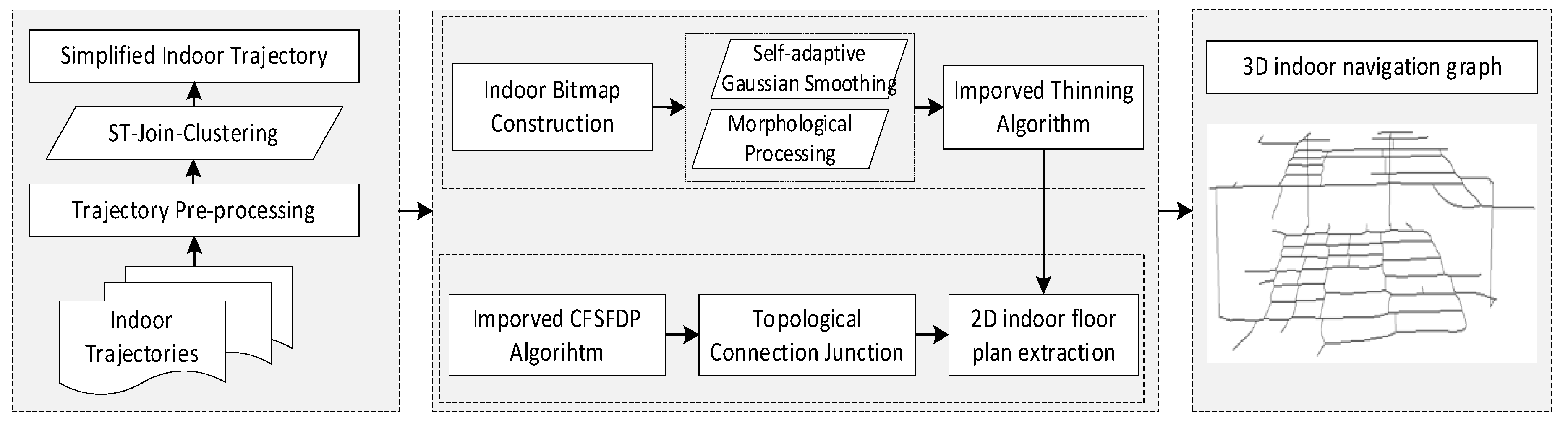
Our proposed approach is composed of the following three steps: indoor trajectory simplification, 2D indoor floor plan extraction and 3D navigation graph construction, as shown in Figure 1. The refined indoor trajectory is handled as the input to the second step and the third step. Finally, we reconstruct the 2D indoor navigation graph and topological connection points into a complete 3D indoor navigation graph.

Indoor trajectory simplification: Data preprocessing methods for the indoor moving objects’ movements were necessarily executed by using many predefined rules in this step. It includes the outlier indoor location points, spatial-temporal constraints, time repetitive or location repetitive points and the minimum number of indoor trajectories. Then, an ST-Join-Clustering algorithm was developed to identify and reduce the stay points, which represents a geographic region where a user stayed over a certain time interval. Finally, we pretreated the original indoor trajectories into a more formal and less redundant representation of users’ movements.

2D indoor floor plan extraction: Due to indoor trajectories having a low frequency, the vector-based outdoor network reconstruction methods [14,15] cannot be easily executed. Our proposed approach adopts a raster-based solution. However, the traditional KDE-based methods [33] were not suitable for generating indoor navigation graphs, because of more noisy data in indoor spaces. We proposed an indoor bitmap construction method based on self-adaptive Gaussian filtering to implement rasterization of indoor spaces using indoor trajectories. Then, we developed a new improved thinning algorithm to extract a 2D indoor floor plan to further optimize the construction of indoor navigation graphs and to reduce the burrs phenomenon.

3D indoor navigation graph reconstruction: Topological connection junctions (e.g., elevators, stairs, escalators) play an important role in the reconstruction of 3D indoor navigation graphs, especially for the complicated indoor space. We took the refined indoor trajectory as an input and adopted a vector-based clustering optimization that estimates the location of the topological connection junctions. Considering that the shapes of density distributions of topological junctions are different and hard to distinguish, we proposed an improved CFSFDP clustering algorithm to identify the 3D topological connection points between two different floors.

3.1. Indoor Trajectory Simplification Step

Different from the outdoor trajectories, indoor moving humans usually spend more time in specific rooms, such as local bars, clothes shops, cinemas, snack bars and so on, to enjoy their lives. This dynamic resulted in the very high number of indoor location points in the fixed region. These location points are often defined as stay points, which represent a region where a moving object stayed over a certain time interval. It has semantic information for some knowledge discovery systems, representing user’s personally meaningful places such as homes, schools, metro stations and hotels, to support many applications for mining interesting locations [41], trajectory recommended systems [42] and so on. In the process of constructing indoor navigation graphs, these stay points have the opposite effect and cause a lot of noise that reduces the precision of indoor navigation graphs.

To overcome the significant impact of redundant stay points, we propose a ST-Join-Clustering algorithm to identify stay points and implemented a trajectory simplification, as inspired by the DJ-Cluster algorithm [43].

Definition 1. 

(Spatial-Temporal neighborhood of an indoor location point $ipt$). The neighbor $STN$ of an indoor location point p, denoted by $STN\left(ipt\right)$, is defined by the following equation:

$$STN(ipt)=\{iqt\in IS|dis{t}_s(ipt,iqt)⩽Eps,dis{t}_t(ipt,iqt)⩽Etm\}$$

(1)

where $IS$ is defined as the set of all indoor location points; $Eps$ is the distance threshold; and $Etm$ is the time interval threshold. For any indoor location point $iqt$, the distance $dis{t}_s$ is less than or equal to $Eps$, and $dis{t}_t$ is less than or equal to $Etm$.

Definition 2. 

(Spatial-Temporal Join). If there are $n$ indoor location points $ipt$ that belong to $STN\left(ipt\right)$ and $STN\left(iqt\right)$ simultaneously, with respect to the threshold $Eps$ and $Etm$, we define $STN\left(ipt\right)$ as joinable to $STN\left(iqt\right)$.

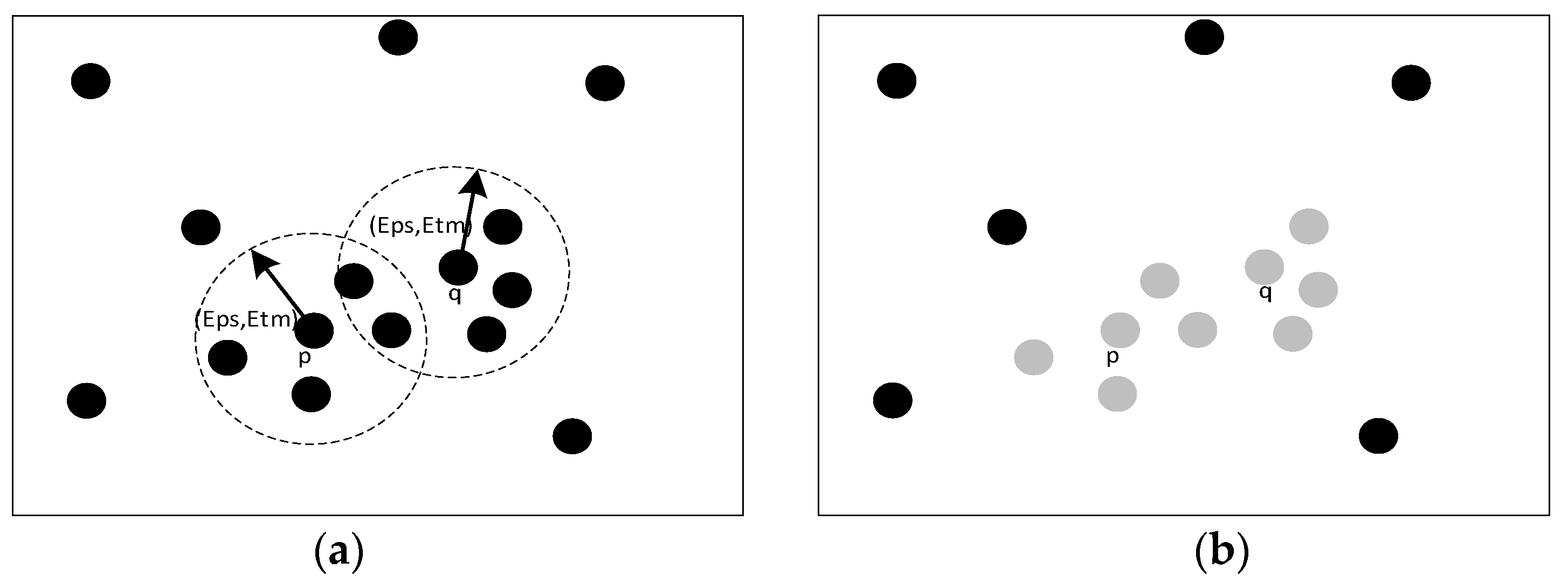
Figure 2 illustrates the process of ST-Join-Clustering.

Algorithm 1 shows the process of the ST-Join-Clustering algorithm. First, it traverses all indoor location points and calculates the spatial-temporal neighborhood of an indoor location point. If the distance and time interval meets the threshold conditions of $Etm$ and $Etm$, all the points in the neighborhood form one cluster. Second, each indoor cluster is then merged with any existing overlapping clusters with respect to $ipt$. Finally, the iterations are completed and there is no new cluster. Moreover, each cluster is disjoined from other clusters.

Algorithm 1 ST-Join-Clustering Algorithm

Input:  Indoor Trajectory Location point $p_i$ Output:  Stay points $SP$ 1. while there is at least one unprocessed indoor point $ipt$ do 2. Compute the spatial-temporal neighborhood $STN\left(ipt\right)$ 3.      if $STN\left(ipt\right)\ne null$ then 4.      else if there is existing cluster $ST{N}_{ex}\left(ipt\right)$ contain the$STN\left(ipt\right)$ then 5.      $Merge(ST{N}_{ex}\left(ipt\right),STN\left(ipt\right))$ 6.      else 7.         Create a new spatial-temporal cluster $STC$ based on $STN\left(ipt\right)$ 8.         $SP.append\left(STC\right)$ 9.      end if 10. end while

Definition 3. 

(Center of Stay Points). After we adopted ST-Join-Clustering to identify clusters, we created a new indoor location point for each cluster, which is defined as $IC\left(x,y,t\right)$:

$$IC\left(x,y,t\right)=\left(\frac{1}{m}{\displaystyle \sum }_{i=0}^m{x}_i,\frac{1}{m}{\displaystyle \sum }_{i=0}^m{y}_i,\left(Min\left\{t_1,t_2,\dots ,t_m\right\}+\frac{\mathsf{\Delta }t}{2}\right)\right)$$

(2)

where $m$ is the number of indoor location points for each cluster. $\mathsf{\Delta }t$ denotes the time interval of each cluster. Figure 3 illustrates an example of the center of stay points.

3.2. 2D Indoor Floor Plan Extraction Step

3.2.1. Indoor Bitmap Construction

In this section, we proposed the indoor bitmap construction method based on self-adaptive Gaussian filtering to implement rasterization of indoor spaces using indoor trajectories. First, the indoor space is divided into a $M\times M$ matrix. Each cell covers a square area. Then, we counted how many indoor location points are in a square cell, as shown in Figure 4.

After the construction, we obtained a raw indoor bitmap where the density of indoor location points was represented by the pixels of the indoor bitmap. However, there is considerable noise in indoor bitmap images. This noise will lead to a significant decrease in the extraction of indoor navigation graphs. Accordingly, we proposed a novel self-adaptive Gaussian smoothing operator to reduce the noise of indoor bitmap.

The Gaussian filter is widely used in image smoothing, which modifies the input image by a convolution with a Gaussian function, in the field of the computed vision and signal processing. The Gaussian smoothing operator is a 2D convolution operator that is used to “blur” images and remove detail and noise. In two dimensions, it is the product of two such Gaussians, and it has the form of:

$$G\left(x,y\right)=\frac{1}{2\pi {\sigma }^2}{e}^{-\frac{x^2+y^2}{2{\sigma }^2}}$$

(3)

where x is the distance from the origin in the horizontal axis, y is the distance from the origin in the vertical axis and σ is the standard deviation of the Gaussian distribution.

The Gaussian template is used to smooth the digital images. $\left(2l+1\right)\times \left(2l+1\right)$ is the Gaussian kernel. The pixel value of the neighbor $\left(2l+1\right)\times \left(2l+1\right)$ matrix is defined as follows:

$$I{H}_{i,j}=\frac{1}{2\pi {\sigma }^2}{e}^{-\frac{{\left(i-l-1\right)}^2+{\left(j-l-1\right)}^2}{2{\sigma }^2}}$$

(4)

The standard deviation $\sigma$ greatly affects the Gaussian kernel. If the $\sigma$ is too small, the weight value of the indoor noncenter pixel’s value is very low and the Gaussian filter has no impact on image processing. In contrast, if the $\sigma$ is too high, the indoor image would lose image details after applying the Gaussian smoothing operator. Hence, we must choose the best $\sigma$ to keep the indoor skeleton maximally connected and preserve the geometry of the indoor image.

The traditional Gaussian filter will select the fixed Gaussian kernel to smooth the indoor image. To maintain the features of indoor image as much as possible in the processing of extracting the indoor graph, we first need to differentiate the internal pixels from the edge pixels of the indoor image. The amount of variation or dispersion of the internal pixels of the indoor images is relatively small, and the standard deviation of the internal pixels of indoor images is also small. Instead, the standard deviation of the edge pixels of indoor images is relatively large. According to this feature, we first calculate the standard deviation $ID$ within the neighbor. Then, the  is selected adaptively based on the $ID$. If $\sigma$ is small, we will choose the smaller Gaussian kernel. If $\sigma$ is large, the larger Gaussian kernel will be adopted. The calculation formula is as follows:

$$ID=\frac{1}{m}\sum {\left(x_{ij}-\overline{x}\right)}^2$$

(5)

$$\overline{x}=\frac{1}{m}\sum x_{ij}$$

(6)

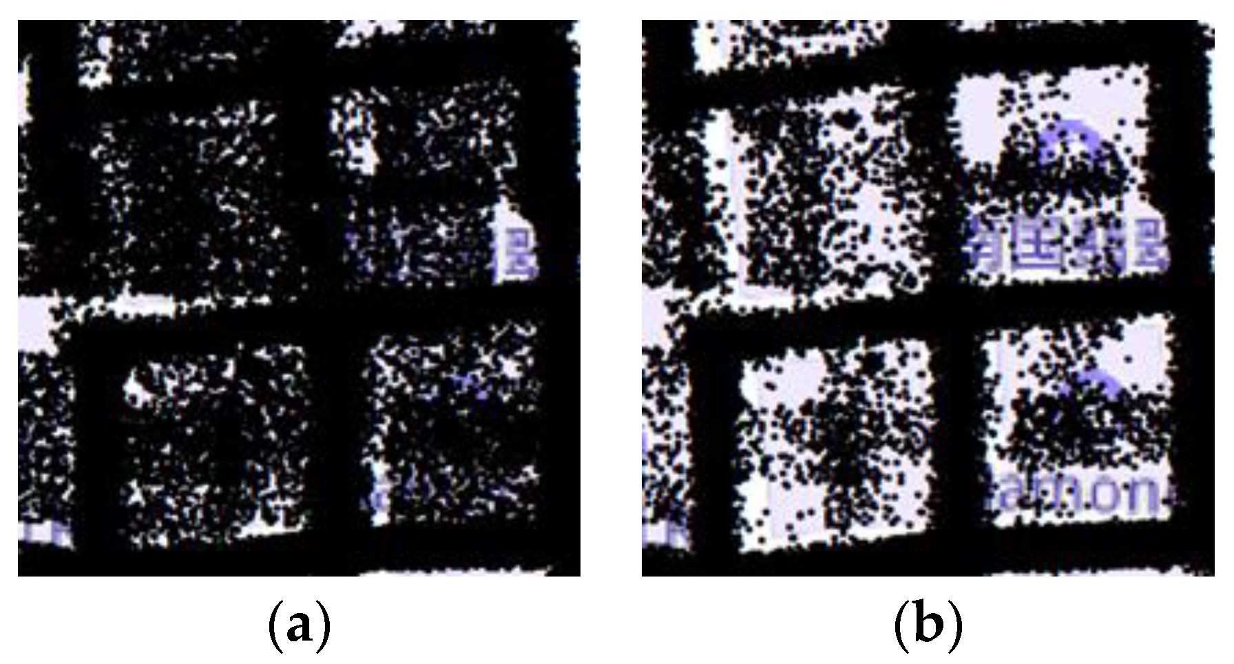
where $m$ is the number of indoor pixels in the neighbor, and $\overline{x}$ denotes the average value. Figure 5 shows an example of indoor bitmap construction.

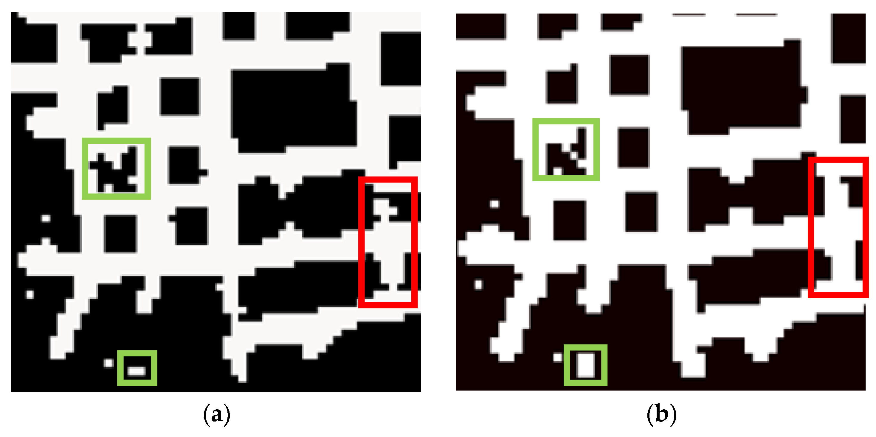
After constructing the indoor bitmap $IBP$, we adopted two morphological opening and morphological closing operators to further erase noises in the images. Next, we will briefly describe the two morphological operations. Morphological opening is the dilation of the erosion of indoor image $IBP$ A by $N\times N$ convolution kernels $CK$. Morphological closing is the erosion of the dilation of indoor image $IBP$ A by $N\times N$ convolution kernels $CK$. The calculation formula is as follows:

$$IBP\circ CK=(IBP\ominus CK)\oplus CK$$

(7)

$$IBP•CK=(IBP\oplus CK)\ominus CK$$

(8)

Generally, in the indoor bitmap, there are some small, jagged lines at the edge of the indoor corridor. We apply morphological opening to remove the sawtooth and obtain a smoother corridor image. Some morphological closing operators are conducted in small, closed spaces such as rooms to reduce the noisy data. After this transformation, a more accurate indoor bitmap is constructed, as shown in Figure 6.

3.2.2. 2D Indoor Navigation Graph Extraction

The thinning algorithm is a useful tool for calculating the skeleton of a binary bitmap in image processing. There are already many thinning algorithms to extract a road network skeleton in outdoor space. However, these common thinning algorithms still need to be improved and further optimized for the construction of indoor navigation graphs. For example, the traditional thinning results cannot ensure the pixel width, and the burrs phenomena are worse. Considering the small indoor space, the indoor navigation graph usually has a more complex structure than an outdoor road network. We introduce a new concept of a pixel’s neighbors binary code and propose a new improved thinning algorithm to compute the 2D navigation graph structure of a single indoor floor, based on the fast-parallel thinning algorithm proposed by Zhang [44]. We describe our algorithm as follows.

Definition 3. 

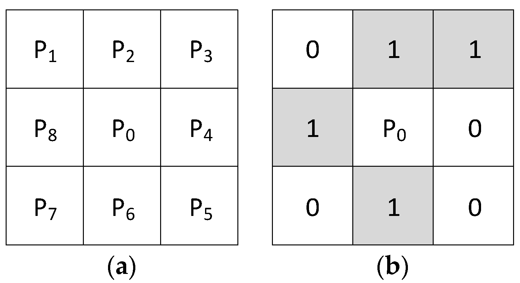
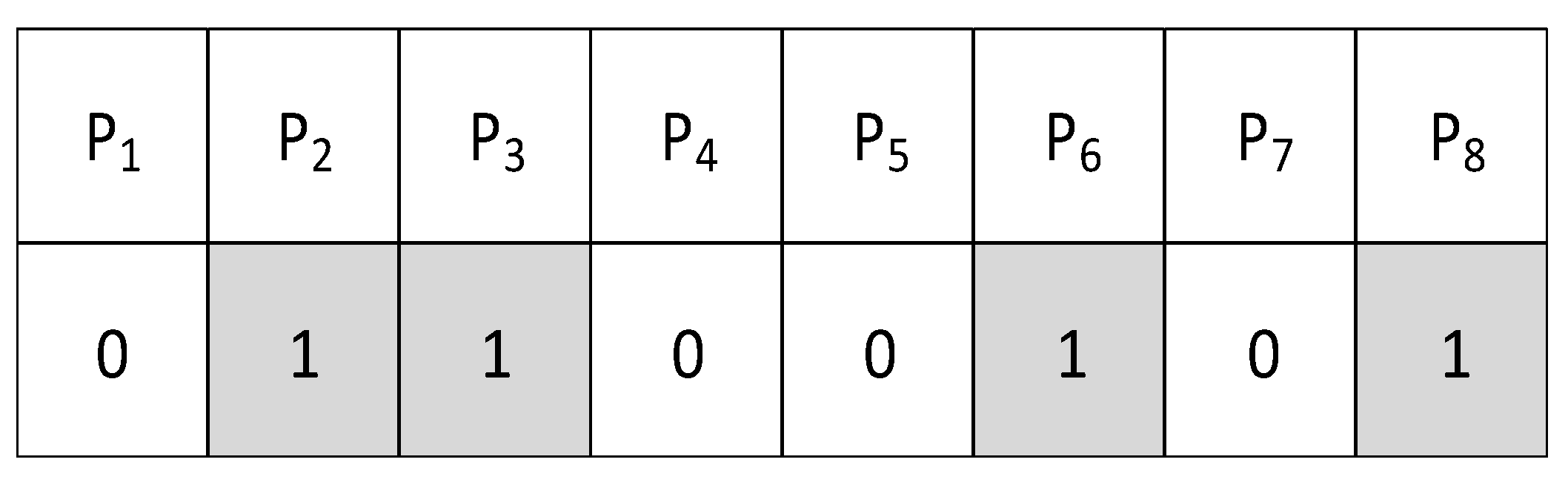
(Eight-connection neighbors of indoor pixel). It is assumed that the neighbors of pixel $INZ\left(P_0\right)$ are $P_1$, $P_2$, $P_3$, $P_4$, $P_5$, $P_6$, $P_7$ and $P_8$, as shown in Figure 7. In addition, when the pixel value of $P_i$ is zero, $P_i$ is defined as the blank point, when the pixel value of $P_i$ is 1, $P_i$ is defined as the target point.

Definition 4. 

(Indoor pixel’s binary code). Figure 8 illustrates an example of binary code $IZB\left(P_0\right)$ for an indoor pixel’s eight-connection neighbors. The code ranges from 0 to 255. The eight-connection neighbors of $P_0$ are transformed into one byte in the clockwise direction. The upper-left pixel $P_1$ is put into the first byte place.

The traditional fast parallel thinning algorithm adopts the following conditions to extract the network skeleton:

(1)

$2⩽INZ\left(P_0\right)⩽6$

(2)

$IZ\left(P_0\right)=1$

(3)

$P_2\times P_4\times P_6=0$

(4)

$P_4\times P_6\times P_8=0$

where $INZ\left(P_0\right)$ denotes the number of pixels among $P_0$. The value of $IZ\left(P_0\right)$ must examine the frequency of target points among the eight-connection neighbors. To overcome the problem of a single pixel width in an indoor space and to keep the skeleton maximally connected, the pattern of target points around eight-connection neighbors are further classified into two categories in our methodology.

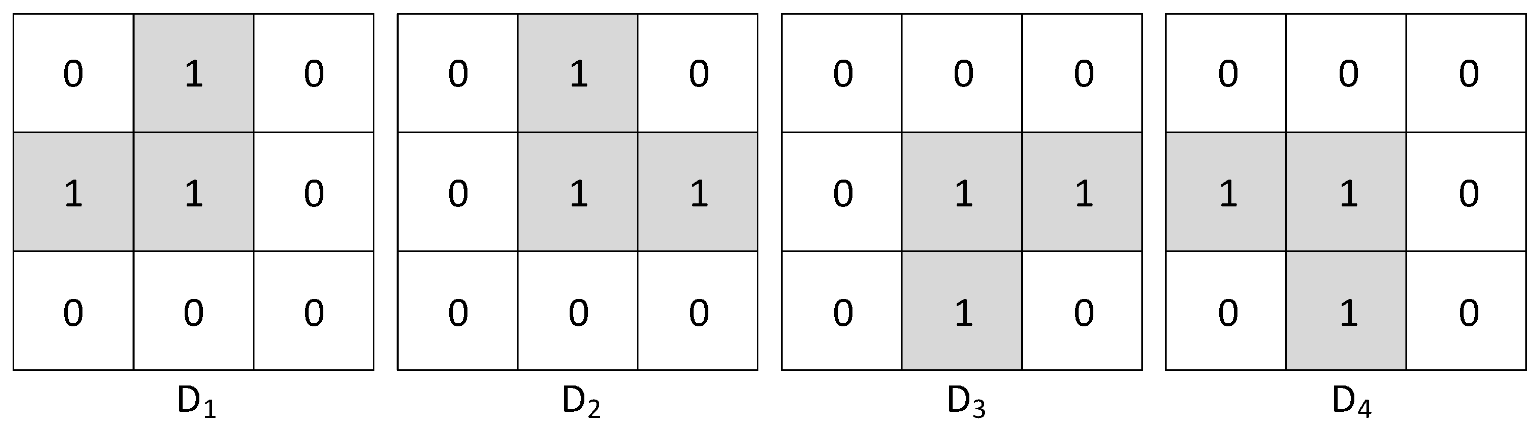
The first category has two target points around eight-connection neighbors, as shown in Figure 9. In all 4 sequence patterns, the target points $D=\left\{D_1,D_2,D_3,D_4\right\}$ are involved in this category. Then, the binary code of indoor pixel $P_0$ may be defined as $IZB\left(P_0\right)\in \left\{5,20,80,65\right\}$.

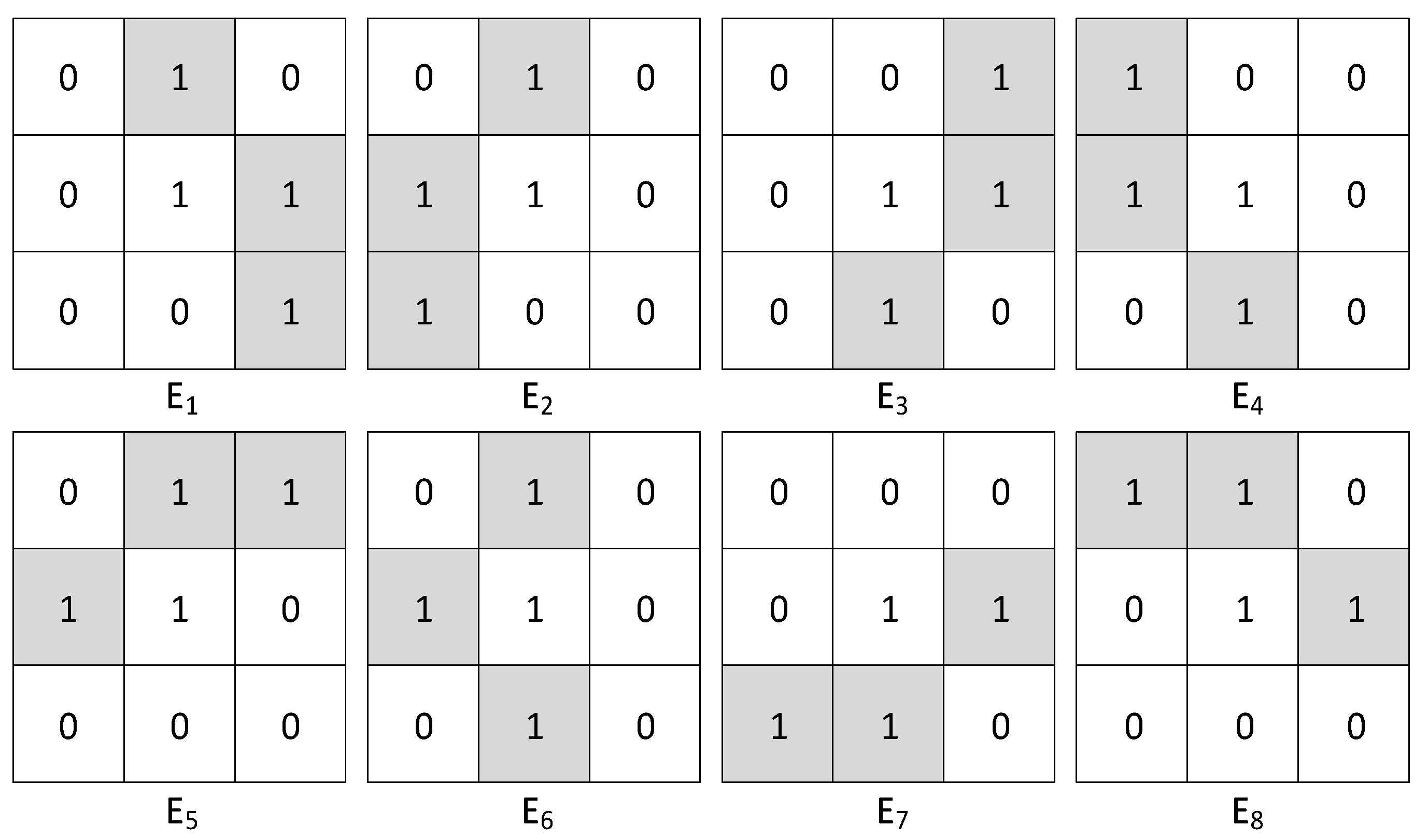
The first category has three target points around eight-connection neighbors, as shown in Figure 10. There are 8 sequence patterns of target points in this category, and it may be defined as $E=\left\{E_1,E_2,E_3,E_4,E_5,E_6,E_7,E_8\right\}$. Then, the binary code of indoor pixel $P_0$ may be defined as:

$$IZB\left(P_0\right)\in \left\{13,22,52,67,88,97,133,208\right\}$$

The optimized fast parallel thinning algorithm introduces new two conditions as follows:

(1)

$IZB(P_0)\in \{13,22,52,67,88,97,133,208\}$

(2)

$IZB\left(P_0\right)\in \left\{5,20,80,65\right\}$

The process of extracting a 2D navigation graph of an indoor space may be defined as $S_n\left(X\right)$:

$$S_n\left(X\right)={\displaystyle \bigcup }_{i=1}^{4}J\left(X,D,E,n,i\right)n=0,1,\cdots ,N$$

(9)

$$\begin{array}{c}J\left(X,D,E,n,i\right)=\{\left(\left(X_n⊝D^i\right)-\left(\left(X_n⊝D^i\right)\circ D^i\right)\right)\cup \left(\left(X_n⊝D^{i+1}\right)-\left(\left(X_n⊝D^{i+1}\right)\circ D^{i+1}\right)\right)\cup \\ \left(\left(X_n⊝E^i\right)-\left(\left(X_n⊝E^i\right)\circ E^i\right)\right)\}\end{array}$$

(10)

$$X_n=X⊝n\left(D^1\oplus D^2\oplus D^3\oplus D^4\oplus E^1\oplus E^2\oplus E^3\oplus E^4\right)n=0,1,\cdots ,N$$

(11)

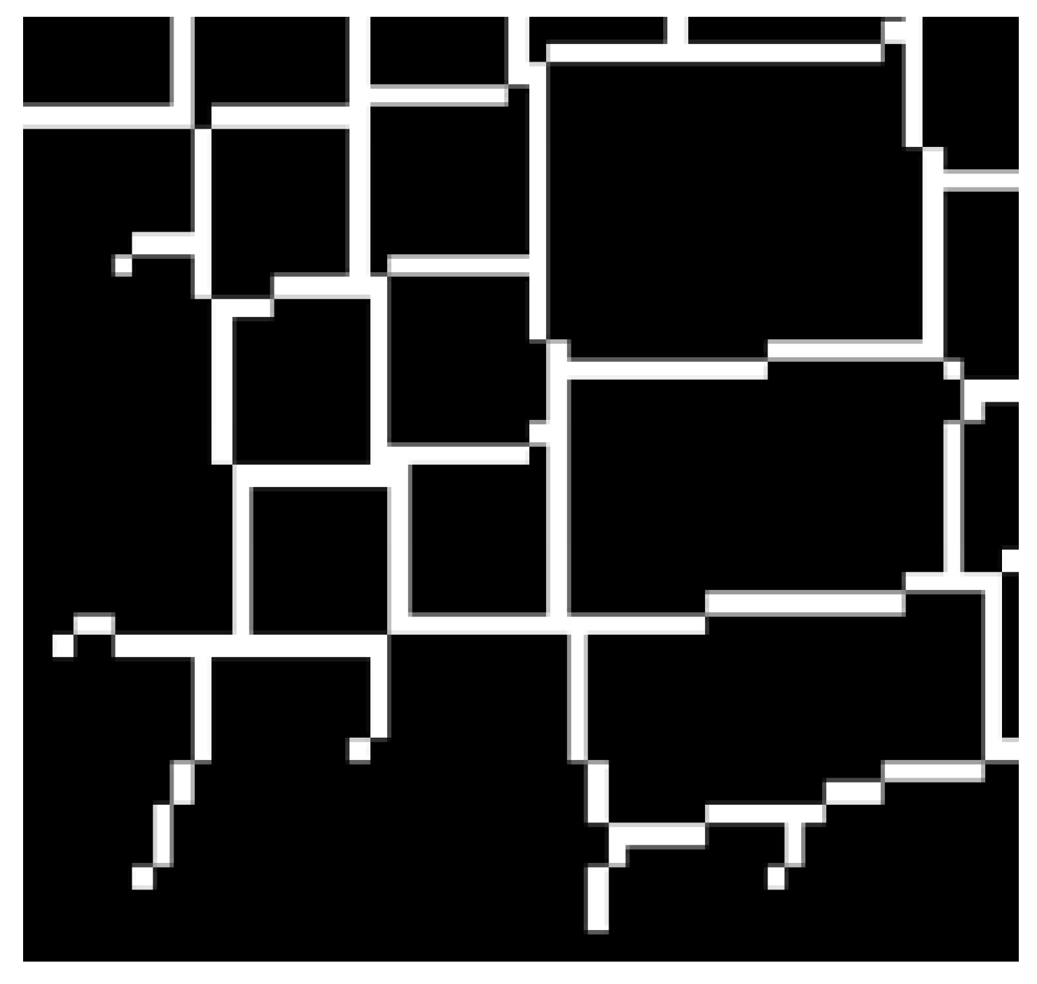
As previously stated, when we iteratively execute the algorithm throughout each indoor pixel, the 2D navigation graph of the indoor space may be extracted. Figure 11 illustrates an example of an indoor navigation graph.

3.3. 3D Indoor Navigation Graph Reconstruction Step

Indoor space usually has a complicated 3D topological structure. Two different floors are connected through points such as elevators, stairs or escalators. In this section, we propose a vector-based 3D navigation graph reconstruction method to capture these topological connection points from crowd-sourced indoor trajectories. We observe that moving objects often spend time waiting around these 3D connection areas because they need to transfer from one floor to another. Inspired by this behavior of moving objects, applying clustering algorithms to indoor trajectories that have removed the impact of stay points in the step of trajectory simplification may be beneficial for identifying connection points.

Clustering has been widely studied and many effective algorithms have been developed, such as ST-DBSCAN [45], K-Means [46] and BIRCH [47]. To select an appropriate clustering algorithm for identifying the 3D connection points, we put forward the following selection criteria: (1) The clustering algorithm should be automated as much as possible, without manually choosing the density threshold. Determining an appropriate threshold in a complicated 3D space is difficult. (2) The clustering algorithm can find different shapes of density distributions. It has a strong robustness of processing cluster centers for different types of indoor topological connection points.

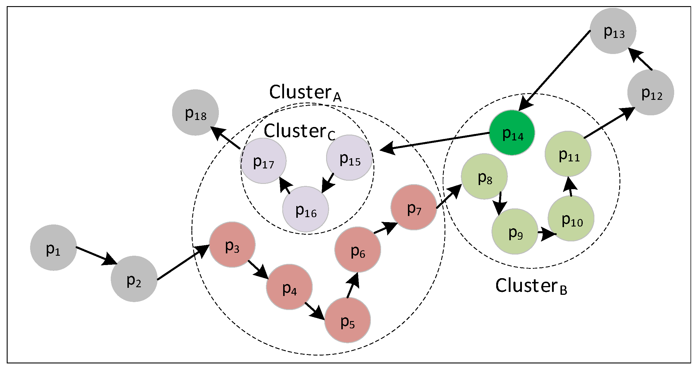
CFSFDP was developed by Rodriguez and Laio [48], and it basically meets our selection criteria. The classical CFSFDP clustering algorithms maintain the advantages of partition-based and density-based clustering algorithms. However, it does not apply to indoor location points with spatial-temporal characteristics because it does not consider the time constraints. Figure 12 shows the clustering results of CFSFDP without time constraints. The clusters A and B are correctly recognized. However, if we consider the sequence and time intervals of indoor location points, the cluster should be split into three clusters: A, B and C.

In our methodology, we proposed improved CFSFDP algorithms with time constraints to identify the 3D topological connection points between two different floors. We now describe the algorithm as follows. We group each simplified indoor trajectory into one floor into a dataset of indoor location points $IP{T}_{floor}$. It is defined as follows:

$$IP{T}_{floor}=\left\{ip{t}_1,ip{t}_2,\dots ,ip{t}_N\right\}$$

$$ip{t}_i=\left(lat,lon,time,floor\right)$$

where $lat$ denotes latitude, $lon$ is the longitude, $time$ denotes the timestamp and $floor$ is the floor identifier in the indoor space.

In the improved CFSFDP, the cluster centers gave the following selection characteristics: (1) The cluster centers have a higher local density than their neighbors. (2) The cluster centers have smaller time interval densities than their neighbors. (3) There is a relatively larger distance between the cluster center and other points within higher densities. Algorithm 2. gives a formal description of our improved CFSFDP with time constraints.

Algorithm 2 The Improved CFSFDP Algorithm

Input:  Indoor Trajectories Output:  The clusters $CS$ 1. Compute the spatial distance matrix $stDisMat$ 2. Compute the time distance matrix $tmDisMat$ 3. $denseArray=null$ 3. while there is at least one unprocessed indoor point $ipt$ do 4.      Compute the local density ${\rho }_i$ and ${\delta }_i$ 5.      $denseArray.append\left({\rho }_i,{\delta }_i\right)$ 5. end while 6. $dentistySort= argsort\left(denseArray\right)$ 7. for each element $ele$ in $dentistySort$ do 8.      Compute the parameter $\gamma =ele.{\rho }_i\ast ele.{\delta }_i$ 9. end for 10. Calculate the number of clusters based on the decision graph $classNum$ 11. $CS=extract\_clustering\left(\gamma ,classNum,stDisMat,tmDisMat\right)$ 12. return$CS$

First, for each indoor location point $ip{t}_i\in IP{t}_{floor}$, we calculate its local density ${\rho }_i$ and its distance ${\delta }_i$ from the indoor location points of higher density:

$${\rho }_i={\displaystyle \sum }_j^N\chi \left(i{d}_{ij}-i{d}_c,i{t}_{ij}-i{t}_c\right)$$

(12)

$$\chi \left(id,it\right)=\{\begin{array}{c}1,id<0,it<0\\ 0,id⩾0,it⩾0\end{array}$$

(13)

where if $i{d}_{ij}<i{d}_c$, and $i{t}_{ij}<i{t}_c$, $\chi \left(id,it\right)=1$. If $i{d}_{ij}⩾i{d}_c$ and $i{t}_{ij}⩾i{t}_c$, $\chi \left(id,it\right)=0$. A very critical component in this processing is the cutoff distance value $i{d}_c$. We calculate the distance $i{d}_{ij}$ and time intervals $i{t}_{ij}$ between any indoor location points as follows:

$$i{d}_{ij}=dis{t}_d\left(ip{t}_i,ip{t}_j\right)$$

(14)

$$i{t}_{ij}=dis{t}_t\left(ip{t}_i,ip{t}_j\right)$$

(15)

Then, the distance sequence $id$ and times interval sequence $it$ are sorted in ascending order:

$$id=\left\{\left(i{d}_1,i{d}_2,\dots ,i{d}_M\right)|i{d}_i⩽i{d}_{i+1}\right\}$$

(16)

$$it=\left\{\left(i{t}_1,i{t}_2,\dots ,i{t}_M\right)|i{t}_i⩽i{t}_{i+1}\right\}$$

(17)

The cutoff distances $i{d}_c$ and $i{t}_c$ are defined as follows:

$$i{d}_c=f\left(id\right)\mathrm{and}i{t}_c=f\left(it\right)$$

(18)

According to the methods of [48], the function is defined as the average number of neighbors being approximately 1 to 2% of the total number of points in the dataset. After the calculation of local density ${\rho }_i$, the local density sequence $\rho$ is sorted in descending order, and its distance ${\delta }_i$ from the indoor location points of higher density is defined as follows:

$$\rho =\left\{\left({\rho }_{q_1},{\rho }_{q_2},\dots ,{\rho }_{q_N}\right)|{\rho }_{q_i}⩾{\rho }_{q_{i+1}}\right\}$$

(19)

$${\delta }_i=\{\begin{array}{c}\underset{q_j}{\min }\left(i{d}_{q_i{q}_j}\right),i⩾2\\ \underset{j⩾2}{\max }\left({\delta }_{q_i{q}_j}\right),i=1\end{array}$$

(20)

According to the decision graph and assumptions, when the indoor location points $ipt$ are larger than the local density ${\rho }_i$ and its distance ${\delta }_i$, the indoor location point $ipt$ is prone to pop up as a cluster center.

To quantitatively define the number of cluster centers, we define a new parameter ${\gamma }_i$. Hence, a higher number of indoor location points will make cluster centers more likely to pop up:

$${\gamma }_i={\rho }_i{\delta }_i$$

(21)

4. Computational Experiments

4.1. Experimental Settings

Our proposed approach was implemented based on Java as the main program language and used Eclipse 4.7 as the development environment. The experiments were conducted on a personal computer with an Intel Xenon CPU E5-2620 v4 @2.10 GHz, 8GB of memory and 512GB solid-state drives, using Windows 10 operating system. The real-world experimental data came from a commercial harmony shopping plaza in Jinan, Shandong Province, China, which contains 4000 indoor trajectories and 5 million location points over a period of two days. The data was provided by the Shanghai Palmap Science and Technology Company Limited Company, an indoor location-based service supplier. The data adopted Wi-Fi indoor positioning systems, and the location errors of points were approximately 3 m.

Table 1. Example of indoor trajectories in the dataset.

ID	Time	X	Y	Floor
000C437231	2017/11/9 10:00:01	135946675	45097102	1
000C437230	2017/11/9 10:00:03	135946016	45097229	1
000C437219	2017/11/9 10:00:04	135946008	45097219	1
000C437267	2017/11/9 12:20:44	135946979	45097371	2

shows an example of an indoor moving object’s movements in the dataset, including fields for the hardware address, latitude, longitude, time and floor. Figure 13 illustrates the number of location points on different floors at different times of the day. The activity time distribution of the indoor moving objects focuses on the section between 9:00 and 22:00.

4.2. Evaluation Approaches

To evaluate the performance of our proposed approach and quantitatively estimate the accuracy of the results, we compared the experimental results with a stand indoor map from the Shanghai Palmap Corporation in a shapefile format. We apply the measurement method of Zhang [26]. The indoor map was split into line segments, and then each line segment was given a 0.2, 0.5 and 0.7 m buffer. We employ an accuracy measure, which is defined as follows:

(1)

Extraction Accuracy $Acc$. The indoor map $SIM=\left\{l{s}_1,l{s}_1,\dots ,l{s}_M\right\}$, and an extracting indoor navigation graph $EIM=\left\{el{s}_1,el{s}_1,\dots ,el{s}_N\right\}$, the extraction accuracy is defined as follows:

$$Acc=\frac{{{\displaystyle \sum }}_{j=1}^{P}length\left(el{s}_j\right)}{{{\displaystyle \sum }}_{i=1}^{M}length\left(l{s}_i\right)}$$

(22)

where $M$ is the line segment number in the stand indoor map, $N$ is the number of line segments in the extraction map, and $P$ is the number of correct results. $length$ represents the function of calculating line segments.

(2)

Topology validation. The topology of the indoor navigation graph will decide whether the construction results can be used in a real-world application. We define topological rules to find topological errors by using the topology rules check toolbox in ArcGIS. Hence, we define a topological accuracy, which is defined as follows:

$$TopoloyAcc=\frac{{{\displaystyle \sum }}_{j=1}^{Q}length\left(el{s}_j\right)}{{{\displaystyle \sum }}_{i=1}^{M}length\left(l{s}_i\right)}$$

(23)

where Q denotes the number of line segments in the indoor navigation graph with the correct topology.

(3)

Baselines. Comparing the road network construction from crowd-sourcing trajectories, few studies were done on generating indoor navigation graphs. Inspired by the ideas of Davies [49] and Kuntzsch [33], we apply the classical KDE for the 2D indoor navigation graph as the baselines to evaluate our proposed approach. In the step of the 3D navigation graph construction, the extracted topological connection points will be compared with the real key points in the stand indoor map. The distance between these points was calculated to evaluate the extraction accuracy in this step.

4.3. Experimental Results

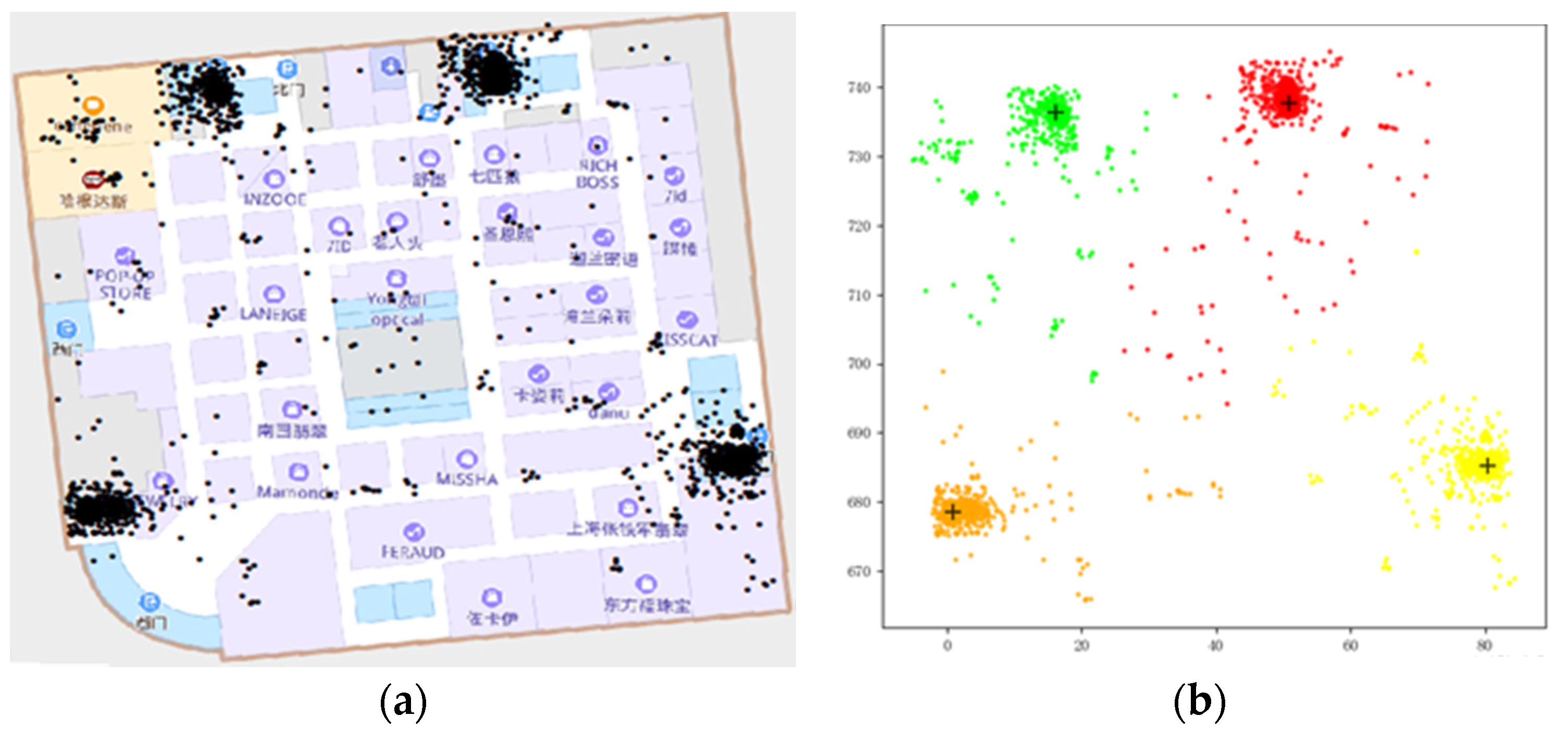
Compared with the original distribution of indoor location points in Figure 14a, the results of the indoor trajectory simplification were refined to a more accurate representation, as shown in Figure 14b. Many stay points were reduced. This result provides the base data for the follow-up extraction algorithms.

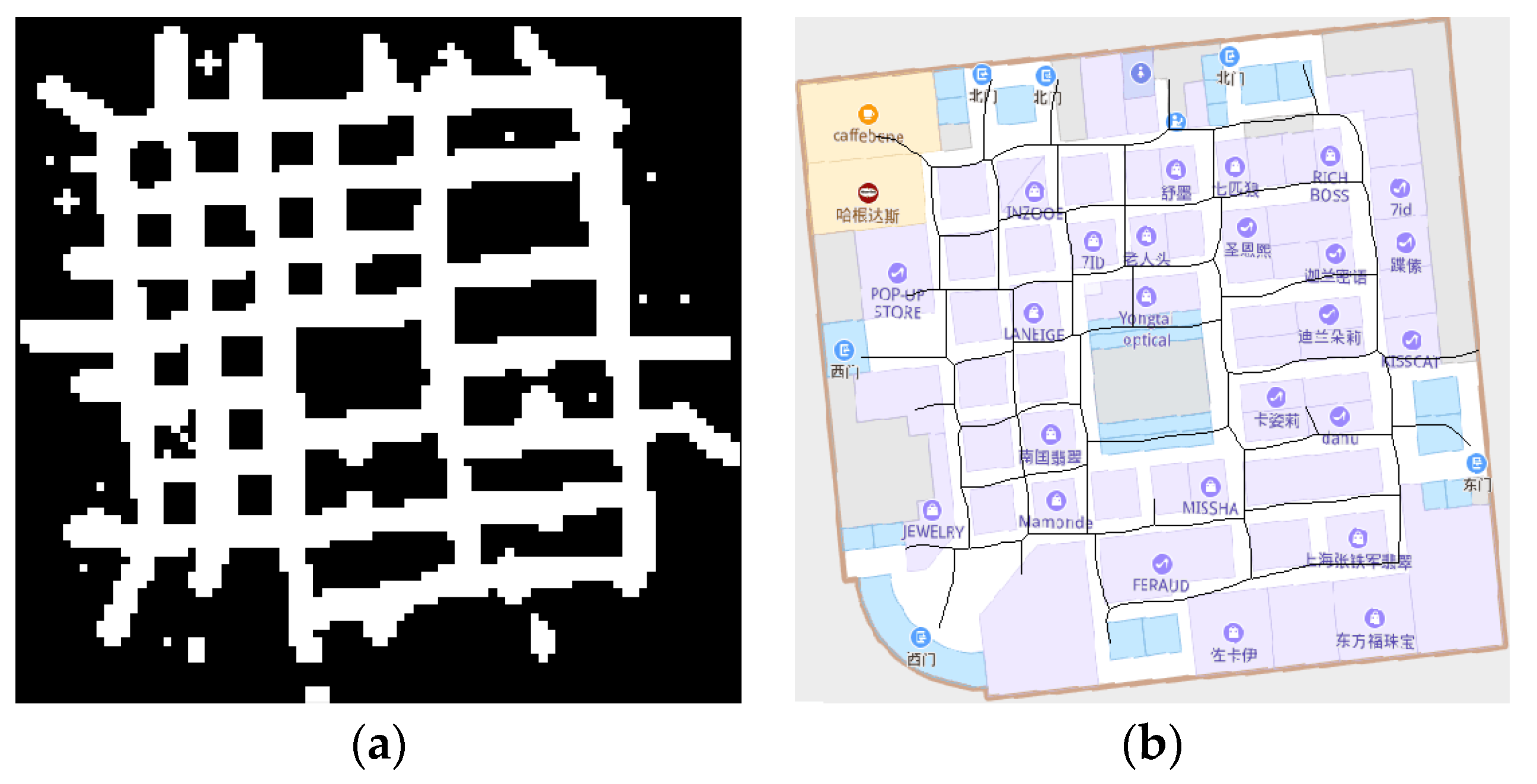
Figure 15a shows the result of the indoor trajectory bitmap construction. Because we adopted self-adaptive Gaussian filter operators, considerable noise in the indoor bitmap images was removed. Meanwhile, some morphological opening and morphological closing operators were conducted to further erase the burrs and noises in the images. Finally, we obtained the 2D navigation graph by using a new improved thinning algorithm, as shown in Figure 15b. However, in an area of fewer indoor location points, our proposed approach cannot capture its structure.

The scalable map generation approach proposed by Davies included four basic stages: generating 2D histogram, deducing the road edges’ positions, computing centerlines and determining the direction, as shown in

Table 2. Experimental results of generating the 2D navigation graph.

	Buffer Size (Meter)			TopologyAcc
	0.2	0.5	0.7
Davies	32.1	66.5	74.1	82.50
Our proposed approach	32.9	68.6	76.6	96.20

. The accuracy of our proposed approach increased by 0.8%, 2.1% and 2.5%. If we only judge the accuracy, the efficiency improvement of our proposed approach is not obvious. That means both approaches could extract some results of the navigation networks. However, after further analysis of topological relations of experimental results, we found that there are more topological errors such as dangling lines and self-intersect in the Davies’s scalable map generation approach,. After the topology validation, the topology accuracy of our proposed approach increased by 13.7%. The main reason is that scalable map generation approach only considers the density of location points. However, more points do not mean more moving objects in the indoor space. Our proposed approach adopted many measurements such as trajectory simplification, self-adaptive Gaussian smooth and morphological operators to reduce these redundancies and errors.

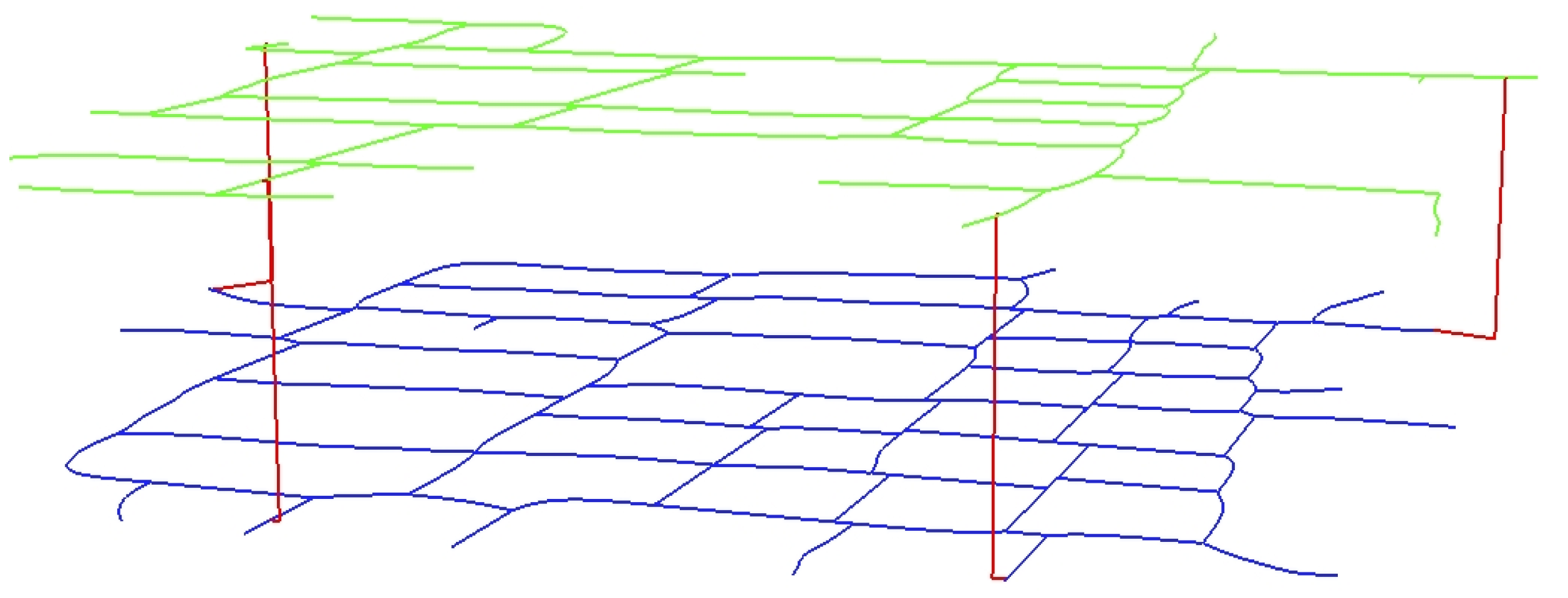
Figure 16 shows the extraction results of topological connection junctions. Our proposed approach only found four cluster areas in the F2 shopping area floor. The cluster areas were near the elevator. This limitation is due in part to the data quality of the indoor location points being lower than the outdoor trajectories. The distances from the extracted points to the real-world positions are 2.14, 2.93, 2.57 and 2.01, respectively. Figure 17 illustrates the results of the generated 3D indoor navigation graph.

4.4. Discussions

This study shows that our proposed approach can construct a 3D indoor navigation graph in a complicated indoor space. However, there are still limitations to our approach that are worthy of discussion.

(1)

Generating indoor navigation graphs by only leveraging crowd-sourcing low-frequency trajectories faces many challenges. Compared with indoor building models and mobile sensor data, the accuracy of an extracted indoor navigation graph is comparatively lower; however, indoor trajectories are timelier and have lower acquisition costs. This study represents a step towards enhancing indoor location-based services by obtaining ubiquitous indoor navigation graphs over larger areas. Moreover, our proposed approach has the advantage of discovering changes in complicated indoor spaces.

(2)

The position error of indoor location points affected the experimental results. If the position error is lower, and the data quality of indoor location points is higher, our proposed approach will achieve a better extraction accuracy. Next, we must perform a deeper analysis of the relationships between the position error and extraction accuracy.

(3)

The extracted results of the 2D and 3D indoor navigation graphs still mainly focus on the corridor or arterial streets. The reason for this focus lies in our proposed approach belonging to a raster-based solution, although we adopted a vector-based improved CFSFDP algorithm to obtain the topological connection points. Inferring the network in an area of fewer location points still faces challenges. More researchers will be inspired and encouraged to benefit from the ubiquitous generation of indoor trajectories.

5. Conclusions

Increasing massive indoor trajectories have provided new opportunities to generate indoor navigation graphs. These trajectories also pose great challenges to indoor navigation graph reconstructions. In this paper, we only leveraged the large-scale and low-frequency indoor trajectories to reconstruct indoor navigation graphs and did not require any other auxiliary information. The automatic indoor navigation graph construction mechanism includes three steps: an indoor trajectory simplification, a 2D Indoor floor plan extraction and a 3D navigation graph construction. To reduce the impact of stay points, a novel ST-Join-Clustering algorithm was developed to refine the collected indoor trajectories to a more accurate representation of indoor objects’ movements. Then, considering the indoor trajectory special characteristics, we proposed an indoor bitmap construction based on self-adaptive Gaussian filtering to transform the indoor trajectories to a smoothing bitmap and developed a new improved thinning algorithm introducing the new concept of a neighbor’s binary code to extract a high-precision 2D indoor floor plan. Finally, topological connection points between two different floors are crucial to constructing a 3D navigation graph. The traditional CFSFDP algorithm is improved to identify these topological key points by adding the time constraints to more effectively adapt to indoor trajectories.

Several directions for future studies are suggested. The location error of indoor trajectories will affect the precision and coverage of the extracted indoor navigation graph. Future research will focus on improving the robustness of our approach to handle different indoor trajectories with various position errors. In addition, the extracted topological connection points mainly focus on the higher density of indoor trajectories. In an area with sparse location points, our proposed approach needs to be improved to solve these dead zones and increase the coverage range.

References

- Ahmed, M.; Karagiorgou, S.; Pfoser, D.; Wenk, C. A comparison and evaluation of map construction algorithms using vehicle tracking data. GeoInformatica 2015, 19, 601–632. [Google Scholar] [CrossRef] [Green Version]
- Klepeis, N.E.; Nelson, W.C.; Ott, W.R.; Robinson, J.P.; Tsang, A.M.; Switzer, P.; Engelmann, W.H. The National Human Activity Pattern Survey (NHAPS): A resource for assessing exposure to environmental pollutants. J. Expo. Sci. Environ. Epidemiol. 2001, 11, 231. [Google Scholar] [CrossRef] [Green Version]
- Diakité, A.A.; Zlatanova, S. Spatial subdivision of complex indoor environments for 3D indoor navigation. Int. J. Geogr. Inf. Sci. 2018, 32, 213–235. [Google Scholar] [CrossRef] [Green Version]
- Vanclooster, A.; de Weghe, N.V.; Maeyer, P.D. Integrating Indoor and Outdoor Spaces for Pedestrian Navigation Guidance: A Review. Trans. GIS 2016, 20, 491–525. [Google Scholar] [CrossRef]
- Yang, L.; Worboys, M. Generation of navigation graphs for indoor space. Int. J. Geogr. Inf. Sci. 2015, 29, 1737–1756. [Google Scholar] [CrossRef]
- Elhamshary, M.M.; Alzantot, M.F.; Youssef, M. JustWalk: A Crowdsourcing Approach for the Automatic Construction of Indoor Floorplans. IEEE Trans. Mob. Comput. 2018, 8, 1523–1536. [Google Scholar] [CrossRef]
- Karimi, H.A.; Ghafourian, M. Indoor routing for individuals with special needs and preferences. Trans. GIS 2010, 14, 299–329. [Google Scholar] [CrossRef]
- Alzantot, M.; Youssef, M. CrowdInside: Automatic construction of indoor floorplans. In Proceedings of the 20th International Conference on Advances in Geographic Information Systems, Redondo Beach, CA, USA, 6–9 November 2012; pp. 99–108. [Google Scholar]
- Qiu, C.; Mutka, M.W. iFrame: Dynamic indoor map construction through automatic mobile sensing. Pervasive Mob. Comput. 2017, 38, 346–362. [Google Scholar] [CrossRef]
- Zhou, B.; Elbadry, M.; Gao, R.; Ye, F. Towards Scalable Indoor Map Construction and Refinement using Acoustics on Smartphones. IEEE Trans. Mob. Comput. 2019, 19, 217–230. [Google Scholar] [CrossRef]
- Zhou Bing Elbadry, M.; Gao, R.; Ye, F. BatMapper: Acoustic sensing based indoor floor plan construction using smartphones. In Proceedings of the 15th Annual International Conference on Mobile Systems, Applications, and Services, Niagara Falls, NY, USA, 19–23 June 2017; pp. 42–55. [Google Scholar]
- Lin, W.Y.; Lin, P.H.; Tserng, H.P. Automating the generation of indoor space topology for 3D route planning using BIM and 3D-GIS techniques. In Proceedings of the International Symposium on Automation and Robotics in Construction, Taipei, Taiwan, 28 June–1 July 2017; pp. 437–444. [Google Scholar]
- Jamali, A.; Abdul Rahman, A.; Boguslawski, P.; Kumar, P.; Gold, C.M. An automated 3D modeling of topological indoor navigation network. GeoJournal 2017, 82, 157–170. [Google Scholar] [CrossRef] [Green Version]
- Lin Will, Y.; Lin, P.H. Intelligent generation of indoor topology (i-GIT) for human indoor pathfinding based on IFC models and 3D GIS technology. Autom. Constr. 2018, 94, 340–359. [Google Scholar]
- Deng, M.; Huang, J.; Zhang, Y.; Liu, H.; Tang, L.; Tang, J.; Yang, X. Generating urban road intersection models from low-frequency GPS trajectory data. Int. J. Geogr. Inf. Sci. 2018, 32, 2337–2361. [Google Scholar] [CrossRef]
- Yang, X.; Tang, L.; Stewart, K.; Dong, Z.; Zhang, X.; Li, Q. Automatic change detection in lane-level road networks using GPS trajectories. Int. J. Geogr. Inf. Sci. 2018, 32, 601–621. [Google Scholar] [CrossRef]
- Tang, L.; Yang, X.; Dong Zh Li, Q.Q. CLRIC: Collecting Lane-Based Road Information via Crowdsourcing. IEEE Trans. Intell. Transp. Syst. 2016, 17, 2552–2562. [Google Scholar] [CrossRef]
- Tang, L.; Yang, X.; Kan, Z.; Li, Q. Lane-Level Road Information Mining from Vehicle GPS Trajectories Based on Naïve Bayesian Classification. ISPRS Int. J. Geo-Inf. 2015, 4, 2660–2680. [Google Scholar] [CrossRef] [Green Version]
- Wang, J.; Wang, C.; Song, X.; Raghavan, V. Automatic intersection and traffic rule detection by mining motor-vehicle GPS trajectories. Comput. Environ. Urban Syst. 2017, 64, 19–29. [Google Scholar] [CrossRef]
- Luo, H.; Zhao, F.; Jiang, M.; Ma, H.; Zhang, Y. Constructing an Indoor Floor Plan Using Crowdsourcing Based on Magnetic Fingerprinting. Sensors 2017, 17, 2678. [Google Scholar] [CrossRef] [Green Version]
- Ahmed, M.; Wenk, C. Constructing Street Networks from GPS Trajectories. Eur. Symp. Algorithms 2012, 7501, 60–71. [Google Scholar]
- Gao, L.; Song, W.; Dai, J.; Chen, Y. Road Extraction from High-Resolution Remote Sensing Imagery Using Refined Deep Residual Convolutional Neural Network. Remote Sens. 2019, 11, 552. [Google Scholar] [CrossRef] [Green Version]
- Gao, R.; Zhao, M.; Ye, T.; Ye, F.; Luo, G.; Wang, Y.; Li, X. Multi-Story Indoor Floor Plan Reconstruction via Mobile Crowdsensing. IEEE Trans. Mob. Comput. 2016, 15, 1427–1442. [Google Scholar] [CrossRef]
- Gao, R.; Ye, F.; Luo, G.; Cong, J. Indoor Map Construction via Mobile Crowdsensing. Smartphone Based Indoor Map Constr. Princ. Appl. 2018, 3–30. [Google Scholar]
- Liang, J.; He, Y.; Liu, Y. SenseWit: Pervasive floorplan generation based on only inertial sensing. In Proceedings of the 2016 International Conference on Distributed Computing in Sensor Systems, Washington, DC, USA, 26–28 May 2016; pp. 26–28. [Google Scholar]
- Khan, A.A.; Donaubauer, A.; Kolbe, T.H. A multi-step transformation process for automatically generating indoor routing graphs from existing semantic 3D building models. In Proceedings of the 3D GeoInfo Conference, Dubai, United Arab Emirates, 11–13 November 2014; pp. 1–20. [Google Scholar]
- Zhang, L.; Thiemann, F.; Sester, M. Integration of GPS traces with road map. In Proceedings of the Third International Workshop on Computational Transportation Science, San Jose, CA, USA, 12 November 2010; pp. 17–22. [Google Scholar]
- Karagiorgou, S.; Pfoser, D. On vehicle tracking data-based road network generation. In Proceedings of the 20th International Conference on Advances in Geographic Information Systems, Redondo Beach, CA, USA, 6–9 November 2012; pp. 89–98. [Google Scholar]
- Cao, L.; Krumm, J. From GPS traces to a routable road map. In Proceedings of the 17th ACM SIGSPATIAL International Conference on Advances in Geographic Information Systems, Seattle, WA, USA, 4–6 November 2009; pp. 3–12. [Google Scholar]
- Huang, J.; Deng, M.; Tang, J.; Hu, S.; Liu, H.; Wariyo, S.; He, J. Automatic Generation of Road Maps from Low Quality GPS Trajectory Data via Structure Learning. IEEE Access 2018, 6, 71965–71975. [Google Scholar] [CrossRef]
- Tang, L.; Ren, C.; Liu, Z.; Li, Q. A Road Map Refinement Method Using Delaunay Triangulation for Big Trace Data. ISPRS Int. J. Geo-Inf. 2017, 6, 45. [Google Scholar] [CrossRef] [Green Version]
- Krylov, V.A.; Nelson, J.D.B. Fast Road Network Extraction from Remotely Sensed Images. Adv. Concepts Intell. Vis. Syst. 2013, 227–237. [Google Scholar]
- Kuntzsch, C.; Sester, M.; Brenner, C. Generative models for road network reconstruction. Int. J. Geogr. Inf. Sci. 2016, 30, 1012–1039. [Google Scholar] [CrossRef]
- Liu, X.; Biagioni, J.; Eriksson, J.; Wang, Y.; Forman, G.; Zhu, Y. Mining large-scale, sparse GPS traces for map inference: Comparison of approaches. In Proceedings of the 18th ACM SIGKDD International Conference on Knowledge Discovery and Data Mining, Beijing, China, 12–16 August 2012; pp. 669–677. [Google Scholar]
- Wang, W.; Yang, N.; Zhang, Y.; Wang, F.; Cao, T.; Eklund, P. A review of road extraction from remote sensing images. J. Traffic Transp. Eng. Engl. Ed. 2016, 3, 271–282. [Google Scholar] [CrossRef] [Green Version]
- Zhao, H.; Comer, M. A Hybrid Markov Random Field/Marked Point Process Model for Analysis of Materials Images. IEEE Trans. Comput. Imaging 2016, 2, 395–407. [Google Scholar] [CrossRef]
- Li, L.; Li, D.; Xing, X.; Yang, F.; Rong, W.; Zhu, H. Extraction of Road Intersections from GPS Traces Based on the Dominant Orientations of Roads. ISPRS Int. J. Geo-Inf. 2017, 6, 403. [Google Scholar] [CrossRef] [Green Version]
- Wang, J.; Rui, X.; Song, X.; Tan, X.; Wang, C.; Raghavan, V. A novel approach for generating routable road maps from vehicle GPS traces. Int. J. Geogr. Inf. Sci. 2015, 29, 69–91. [Google Scholar] [CrossRef]
- Munoz-Organero, M.; Ruiz-Blaquez, R.; Sánchez-Fernández, L. Automatic detection of traffic lights, street crossings and urban roundabouts combining outlier detection and deep learning classification techniques based on GPS traces while driving. Comput. Environ. Urban Syst. 2018, 68, 1–8. [Google Scholar] [CrossRef] [Green Version]
- Aly, H.; Basalamah, A.; Youssef, M. Map++: A crowd-sensing system for automatic map semantics identification. In Proceedings of the 2014 Eleventh Annual IEEE International Conference on Sensing, Communication, and Networking, Singapore, 30 June–3 July 2014; pp. 546–554. [Google Scholar]
- Zheng, Y.; Zhang, L.; Xie, X.; Ma, W.-Y. Mining interesting locations and travel sequences from GPS trajectories. In Proceedings of the 18th International Conference on World Wide Web, Madrid, Spain, 20–24 April 2009; pp. 791–800. [Google Scholar]
- Ashbrook, D.; Starner, T. Using GPS to learn significant locations and predict movement across multiple users. Pers. Ubiquitous Comput. 2003, 7, 275–286. [Google Scholar] [CrossRef]
- Zhou, C.; Frankowski, D.; Ludford, P.; Shekhar, S.; Terveen, L. Discovering Personally Meaningful Places: An Interactive Clustering Approach. ACM Trans. Inf. Syst. 2007, 25, 212–242. [Google Scholar] [CrossRef]
- Zhang, T.Y.; Suen, C.Y. A fast parallel algorithm for thinning digital patterns. Commun. ACM 1984, 27, 236–239. [Google Scholar] [CrossRef]
- Birant, D.; Kut, A. ST-DBSCAN: An algorithm for clustering spatial–temporal data. Data Knowl. Eng. 2007, 60, 208–221. [Google Scholar] [CrossRef]
- Likas, A.; Vlassis, N.; Verbeek, J.J. The global k-means clustering algorithm. Pattern Recognit. 2003, 36, 451–461. [Google Scholar] [CrossRef] [Green Version]
- Zhang, T.; Ramakrishnan, R.; Livny, M. BIRCH: A new data clustering algorithm and its applications. Data Min. Knowl. Discov. 1997, 1, 141–182. [Google Scholar] [CrossRef]
- Rodriguez, A.; Laio, A. Clustering by fast search and find of density peaks. Science 2014, 344, 1492–1496. [Google Scholar] [CrossRef] [Green Version]
- Davies, J.J.; Beresford, A.R.; Hopper, A. Scalable, Distributed, Real-Time Map Generation. IEEE Pervasive Comput. 2006, 5, 47–54. [Google Scholar] [CrossRef]
Figure 1.
Architecture of the proposed approach.
Figure 2.
An example of ST-Join-Clustering. (a) indoor location points; (b) clustering results.
Figure 3.
An example of stay points. (a) trajectory points; (b) center of stay points.