
A Cellular Automata Model for Integrated Simulation of Land Use and Transport Interactions


1
Spatial Policy and Analysis Laboratory, Manchester Urban Institute, The University of Manchester, Manchester M13 9PL, UK
2
CITTA, Department of Civil Engineering, University of Coimbra, 3030-790 Coimbra, Portugal
3
Centre of Land Policy and Valuation, Technical University of Catalonia, 08028 Barcelona, Spain
*
Author to whom correspondence should be addressed.
ISPRS Int. J. Geo-Inf. 2021, 10(3), 149; https://0-doi-org.brum.beds.ac.uk/10.3390/ijgi10030149
Submission received: 30 December 2020
/
Revised: 22 February 2021
/
Accepted: 1 March 2021
/
Published: 8 March 2021
(This article belongs to the Special Issue Measuring, Mapping, Modeling, and Visualization of Cities)
Abstract
:Cellular automata (CA) models have been used in urban studies for dealing with land use change. Transport and accessibility are arguably the main drivers of urban change and have a direct influence on land use. Land use and transport interaction models deal with the complexity of this relationship using many different approaches. CA models incorporate these drivers, but usually consider transport (and accessibility) variables as exogenous. Our paper presents a CA model where transport variables are endogenous to the model and are calibrated along with the land use variables to capture the interdependent complexity of these phenomena. The model uses irregular cells and a variable neighborhood to simulate land use change, taking into account the effect of the road network. Calibration is performed through a particle swarm algorithm. We present an application of the model to a comparison of scenarios for the construction of a ring road in the city of Coimbra, Portugal. The results show the ability of the CA model to capture the influence of change of the transport network (and thus in accessibility) in the land use dynamics.
1. Introduction
Land use and transport are two areas of urban planning that share many common attributes and mutually exert a continuous interdependency that encompasses a high level of complexity. Land use and transport (LUT) interaction has been an intensive topic of research, combining planning, transport and economic theories and making use of different approaches that aim to analyze and simulate the interdependencies of the two areas. Many studies were developed around this topic with a strong focus on theoretical and more operational modeling [1,2,3,4,5].
Cellular automata (CA) models are among the most researched urban simulation models. Along with other approaches to simulate urban systems, such as agent-based models, system dynamics or discrete choice models, CA models are capable of capturing spatial interactions, but perhaps less so in dealing with transport and its impact in urban change. For this reason, CA models need to be coupled with dedicated transport models to capture LUT interactions. The literature indicates some examples of parallel calibration of CA and transport models, but it is absent of cases where both models are fully integrated.
CA models have been under intensive research for the past two decades. CA is a very simple mathematical concept, introduced by Von Neumann and Ulam [6,7], that simulates the evolution of a system under a set of rules and can be represented in a given space. The conceptual definition of a CA includes two main concepts: (1) an automaton, which is “a processing mechanism with characteristics that change over time based on its internal characteristics, rules and external input” [8], and (2) a partition of space, the cell, which has a given state (e.g., occupied or unoccupied) that can change over time.
In practical terms, a CA model is based on a discrete set of spatial units: the cells that together form a cell space. Each cell takes a given (cell) state from a finite set of states. Time is considered in a discrete manner. Each cell, which works as an automaton, then may or may not experience state changes over time, according to a finite set of transition rules that can be of various types (deterministic, stochastic, unconstrained or constrained). State transition results from the application of these rules to each cell, considering the neighboring cells.
Waldo Tobler introduced the concept of CA to geography by defining a series of geographical models that dealt with space and time dynamics in different ways [9]. His consideration of a CA model allowed the modeling of what he has called the first law of geography, which states that everything is related to everything else, but closer things are more related than distant things [10]. The intrinsic spatial character of CA models makes them quite suitable for analyzing land use change, in which transport and accessibility play an obvious key role.
Despite examples of models where CA were coupled with transport models in parallel calibration procedures with retro-feed loops (as in [11]), there are no records of full integration of a transport model within the core structure of a CA model. In LUT models, the aim of capturing the complex interdependencies between land use and transport recommend the integrated calibration of their parameters.
The aim of our research is to show the feasibility of the integration of CA and transport models with a combined calibration to capture the interdependencies of change in both land use and the transport system. We present a CA model in which accessibility is not just an exogenous cell attribute, but it is calculated and calibrated considering travel times over a real road network, thus transforming accessibility into an endogenous variable of the CA model, allowing the effective and integrated calibration of drivers of land use and transport.
We test our model’s capacity to deal with change in land use and transport using a case study in the municipality of Coimbra, Portugal. We use two scenarios that consider the possible construction of a new ring road to explore the capacity of the model to capture the interactions between land use change and changes in the transport system. Our scenarios were designed to explore the performance of our model and are not meant to be used in a real planning process. Nonetheless, our results were presented and discussed at a research workshop, where planning officials and decision makers discussed with modelers the value and potential of these tools.
Following the introduction, Section 2 presents a brief review of the relevant literature on CA and CA models that deal with land use and transport interactions. Section 3 presents a description of the model with its formulation and calibration procedure. Section 4 is dedicated to presenting the results for the application of the model to simulate different scenarios for the construction of an important urban road in the city of Coimbra, Portugal. Finally, Section 5 presents the discussion about the results and about the inclusion of accessibility in CA models, as well as its potential and limitations.
2. A Brief Literature Review of Cellular Automata and Transport Models
CA models are, despite their conceptual simplicity, one of the most capable tools to simulate any kind of phenomena with an intrinsic spatial nature. The works of Von Neumann and Ulam [7,12] and later of Tobler [9] were the foundations for a period of intensive theoretical development that gave birth to the first applications of CA in both theoretical instances and real-world case studies [13,14,15,16]. These theoretical foundations boosted numerous variations and improvements to geographic CA models that are now widely used for simulating increasingly more complex problems [17,18,19,20,21,22]. The vast majority of these applications use regular cells derived from remotely sensed imagery, and even today, there is only a minority of studies that have considered irregular cellular fabrics [23,24,25,26,27,28,29,30,31,32,33]. This is mainly due to the practicalities of operating raster images against the complexities of dealing with complex topologies in vector models.
The ability CA models have to integrate spatial change and neighborhood effects (illustrating Tobler’s first law of geography [10]) suggests their effectiveness in the simulation of the complex interdependencies of spatial phenomena. By being a privileged tool to model spatial interactions—as generically defined in Tobler’s first rule—CA models are conceptually well suited to deal with changes in land use and transport and their complex relationships, as both depend on spatial interactions that drive the correspondent demand for land and for accessibility.
Understanding changes in land use and transport implies the analysis of measures of the level of performance of the transport system and its implications in land use demand. Accessibility is a complex concept and can be defined and measured in multiple ways [34]. One definition, given by Dalvi, identifies “the ease with which any land use activity can be reached from a location, using a particular transport system” [35]. Bhat et al. defined accessibility as a “measure of the ease of an individual to pursue an activity of a desired type, at a desired location, by a desired mode, and at a desired time.” [36] Bertolini et al. defined accessibility as “the amount and diversity of places that can be reached within a given travel time and/or cost” [37]. These definitions highlight activities and their land use and locations as an origin and a destination, the time to travel from and to these locations and the modes as the key components of land use and transport interactions.
Accessibility has therefore been classified as a major driver of urban growth for a long time. A significant number of models that simulate urban growth have different methods to incorporate accessibility and its interdependent effects with a series of other factors, such as land price or household and activity location, just to name a few [1,38,39]. A large number of CA models of land use change incorporate some form accessibility in their formulations, with leading authors acknowledging that accessibility is a key driver of land use change (for a list of CA models that consider some sort of accessibility measure as a driver of urban change, see Table 7 of Santé et al. [40]).
Accessibility is usually included as one of the components in the formulation of CA transition rules, which play the role of the engine that drives CA evolution. However, the majority of these models consider accessibility as a simple cell attribute, defined as the linear distance from a cell to the nearest road or rail (and sometimes the airport) infrastructure [17,24,41,42,43,44,45,46,47,48]. This somewhat simplistic approach discards the effects that infrastructure capacity and travel demand have on the performance of the transport system and their consequences on land use. Other models use a parallel calibration procedure for the land use model based on CA and for the transport model using, for example, the four steps transport model [11,49] or existing dedicated transport models [50]. This lack of full integration between CA models and transport models may be a consequence of the difficulties of calibrating both models as a single model due to the very high number of model parameters.
CA models do not focus on simulating the performance of transport systems, being good at simulating land use change. It is, however, possible to use CA to deepen the integration of land use simulation with more explicit transport models that can provide more elaborate measures of accessibility. These measures of accessibility can include infrastructure capacity, travel demand or multimodal systems, thus capturing the complexity of the land use and transport interaction.
3. Model Formulation
Our CA model was designed to maintain the simplicity of the original CA concept. The model was programmed as a standalone application for Windows OS using the Visual Basic 6 programming language. This section presents the different components of the model.
The cell is the first of the five key CA components. Our model uses irregular cells that aim to simulate real-world irregular spatial partitions. The cells are designed considering census units which take into account urban form (i.e., the most relevant urban features such as streets, buildings or topographic features), thus combining form and reliable data about population or employment. The neighborhood, another key component of CA, is a parameter (δ) calibrated by the model. It is a radial distance and represents the extent to which spatial interactions between land uses are considered to influence cell state transition. By considering the neighborhood as a calibration parameter (and not as a user-defined measure, as the majority of CA models do), the model is more representative of the importance of spatial interactions in land use dynamics. The set of cell states includes six aggregate cell states (or land use classes): urban low density (UL) and urban high density (UH), which aggregates all the land uses located inside urban areas, including public facilities and public spaces; non-built urban areas (XU), which are empty areas that can be developed; industry (I); non-built areas for industrial uses (XI); and areas where urbanization and construction of any type is highly or totally restricted (R). The transition rules are another component of the CA model which play a key role, as they simulate the way the system evolves. The model uses a measure of state transition potential that is used for selecting which cells will change states at each simulation step. The higher the transition potential for a given state (land use) located in a given cell at a given time step t is, the more probable it is for this cell to change to that given state. The potential function computes a weighted value of accessibility, land use suitability and the neighborhood effect, considering a number of calibration parameters affected by a stochastic function to include random decision patterns:
where for each cell i from the set of cells C, and for each state s from the set of states S, Pi,s is the transition potential for state s of cell i; Si,s is the land use suitability value for state s of cell i; Ai is the accessibility value of cell i; Ni,s is the neighborhood effect for state s of cell i considering its neighborhood Vi; νP is the calibration parameter for land use suitability; χP is the calibration parameter for accessibility; θP is the calibration parameter for the neighborhood effect; and ξ is the stochastic parameter. Land use suitability is a binary value that has a value of one if a cell is suitable for a given land use and zero otherwise, as defined by land use regulations in force, representing planning decisions.
Our CA model is designed to be coupled with any transport model that simulates the transport system, using an aggregated value of accessibility per cell that is then used in the CA transition potential as indicated in Equation (1). In this application, and due to the lack of available data for public transport for the case study, we have modeled the road network and its hierarchy to compute travel times to the main urban services and employment centers. Accessibility is used as the aggregate transport indicator, and it is measured by a function of cumulative opportunities considering the travel time between cells (defined by their centroids), measured over the road network considering its hierarchical structure as follows:
where f(T*i) is an impedance function of an aggregate measure of the travel time that differentiates the relative importance of access to where employment or the main urban functions (services, business and public facilities) are located. This function is given by
where Ti,C is the travel time from cell i to the municipality’s main city or town; Ti,V is the travel time from cell i to the closest second-tier town or village in the municipality (simulating smaller administrative units like civil parishes); Ti,In is the travel time from cell i to the industrial site n located in the municipality (out of all industrial sites N); and αA, βA and γA are calibration parameters.
The neighborhood effect Ni,s simulates the spatial interaction between each pair of land uses and is an aggregate value of the interactions Ni,s|j,r between the states s and r, located in two neighboring cells i and j. It is calculated through the following expression:
where the neighborhood effect Ni,s is the sum of the interactions Ni,s|j,r between state s in cell i and all the states of neighboring cells j that belong to neighborhood Vi, considering the neighborhood distance parameter δ (which means that attraction or repulsion will only be taken into account if the cell is located within the neighborhood Vi), and di,j is the distance between cells i and j.
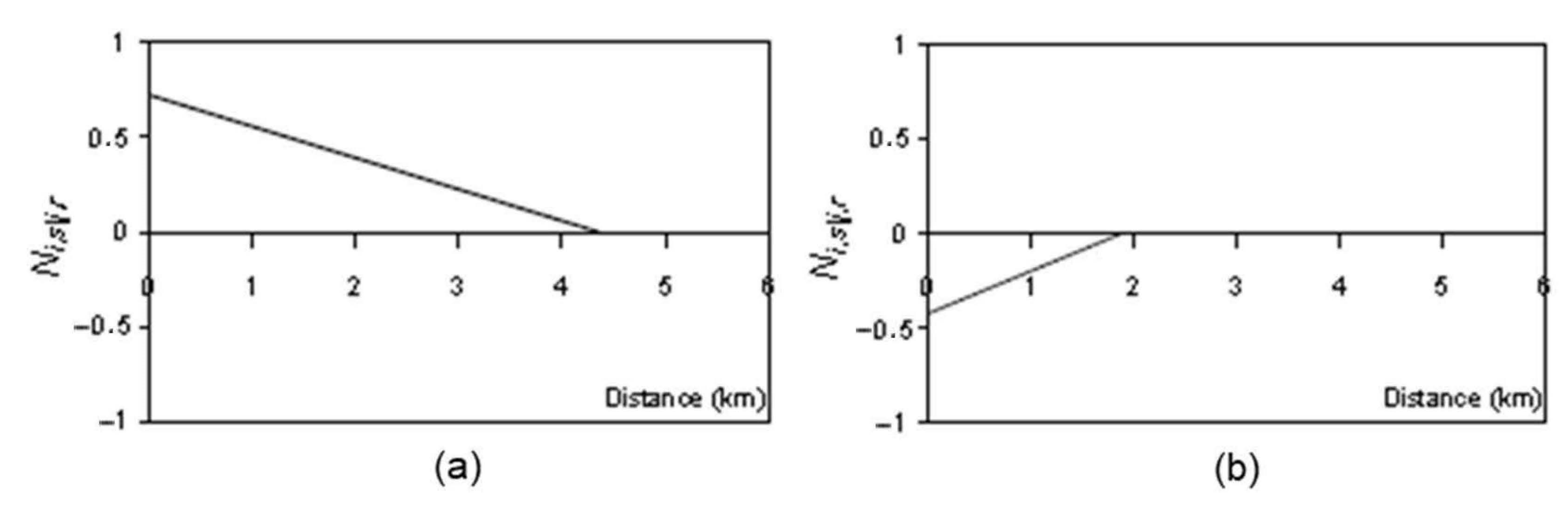
These interactions represent the attraction or repulsion that each pair of cell states mutually exerts. They have a normalized value, ranging from 0 if two cell states do not interact up to +1 if they exert maximum attraction (e.g., cell states UL and R, as depicted in Figure 1a) or from −1 if two land uses exert maximum repulsion (e.g., cell states I and UL, as depicted in Figure 1b) to 0 if they do not interact. These linear functions decay from the maximum value (of attraction or repulsion) at a distance of zero between two cells (with the two cell states) to 0 at a distance where interaction between the cell states in the two cells is no longer observed. The neighborhood effect for a given cell is the sum of all the neighborhood interactions of this cell with all its neighboring cells within its own neighborhood Vi.
Land use demand is proportional to the increase of population and employment, as well as to the variation of built-up areas. We have considered that land use demand varies in time due to the variation of the average built-up area per inhabitant, which tends to include larger housing units with more public spaces and facilities, along with a decrease in the size of households. To represent this variation, we considered a measure of built-up density that took into account the variation of the population and employment, along with the need for space for the corresponding land uses. The use of this measure without constraint would lead to a quick allocation of new developments in cells with higher potential values and more vacant land. Larger cells with higher transition potentials would attract a larger amount of development, eventually leaving no need for new developments elsewhere. The model has a mechanism to tackle this attractiveness of larger cells. Land demand is balanced using a standard logit model that distributes the demand while considering the existent land supply. The logit is applied to the value of the potential P*i,s considering a control variable αL calibrated by the model:
where P*i,s is the value of transition potential in cell i for state s; αL is the logit parameter; and e is the Euler number.
Model performance is assessed using contingency matrices and the corresponding kappa index (see Couto [51] for a comprehensive definition of the measure proposed originally by Cohen [52]). The use of kappa statistics has been the subject of strong academic debate. An indicative sample of the ongoing debate can be illustrated by Congalton and Green [53] advocating for its utility and Pontius and Millones [54] providing evidence of the problems and lack of accuracy of kappa when compared with other metrics derived from contingency matrices. Our decision to use kappa statistics derives from the possibility of establishing some degree of comparison with the overall performance of other CA models (for example, Kang et al. [55], Grinblat, Gilichinsky and Benenson [56] and Petrov, Lavalle and Kasanko [57]).
We have used a modified measurement of kappa (the kMod) that does not take into consideration cell states that cannot change state:
where n is the total number of elements in the contingency matrix, mij is a generic element of the matrix, S is the finite set of cell states and R is the land use class that cannot change.
Some land uses (for example, cell state R, where construction is totally restricted) cannot change but still influence the land use dynamics. The consideration of cells with cell state R for the calculation of the kappa index would produce an overestimation of similarity, as they have the same state in the simulation and in reality. This innovation has been applied in other models [58] and given good results in previous applications of our model [59].
Model calibration uses an optimization procedure called particle swarm (from now on referred to as PS) with the goal of producing an extensive search of the set of calibration parameters that optimize the fitness function chosen for the model (maximizing the value of kMod). It simulates the movement of a group of individuals toward some goal, where the success of each individual influences its own searches and those of their peers [60]. For an in depth reading about PS, see Parsopoulos [61].
The use of PS to calibrate CA models is not common and is usually applied in cases where the number of calibration parameters is considerably high. Pinto et al. [62] have used PS for calibrating a CA model based on a transition potential applied to small urban areas. Feng et al. [63] and Liao et al. [64] developed more traditional CA models based on regular cells and probabilistic transition rules calibrated by a PS algorithm.
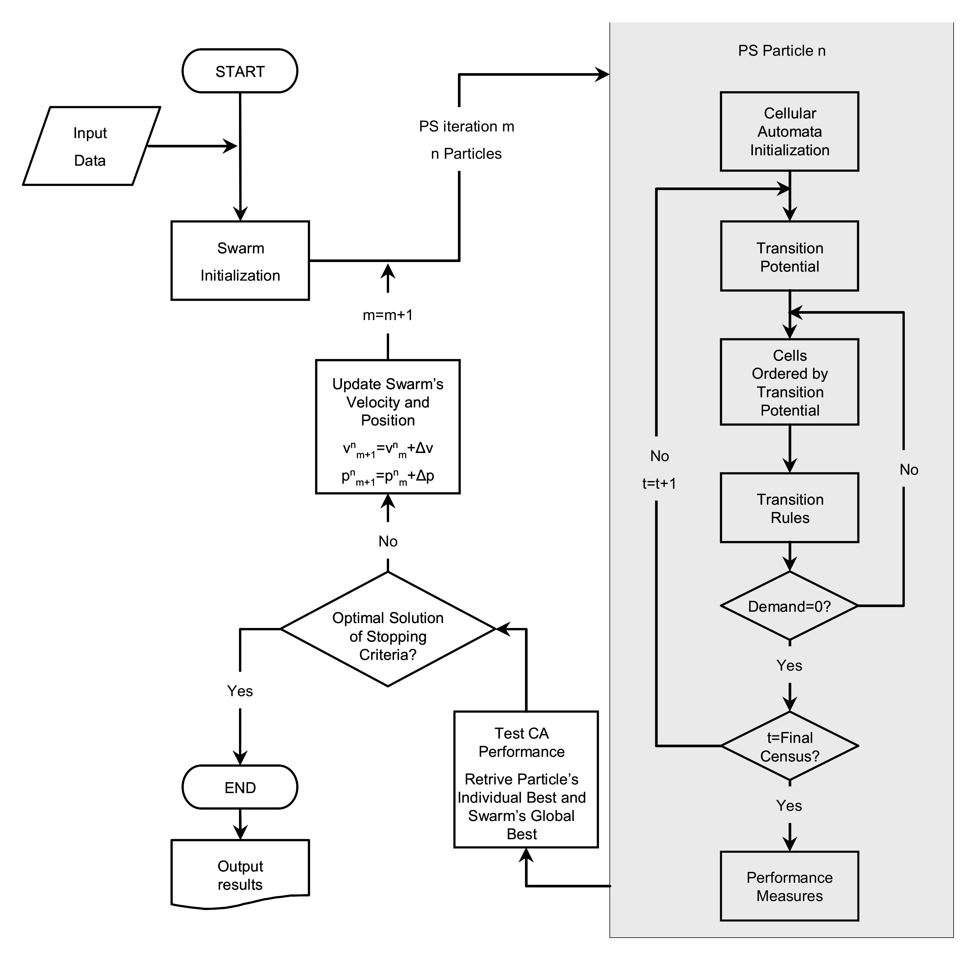
Our implementation of the PS algorithm contains the CA model and searches for an optimal set of calibration parameters for the CA model, as depicted in Figure 2. Each particle is an admissible point of the space of the solutions of the CA model, and the swarm of particles (different admissible points of the solution space) flies along a series of iterations until a given stopping criterion is met. PS has a very simple mathematical formulation based on the position and velocity of the particles in the space of the solutions, which are updated for every iteration. The CA model runs with the set of calibration parameters of each particle in every iteration, and a value of kMod is calculated, being used as the fitness function for the optimization procedure. The process is repeated until the difference between two iterations is smaller than a given threshold. A detailed explanation of our implementation of the PS algorithm to calibrate CA models can be found in Pinto et al. [62].
4. Model Application and Results
The model was applied to a real-world case study to simulate the impact on urban growth of the construction of an important ring road in the urban area of Coimbra, Portugal. The goal was to use this application to exemplify the potential use of the model for scenario evaluation. The model was calibrated for a set of reference data that included census data on demographics and employment for the years 1991 and 2001 and considered the approved municipal master plan, legally in force by 2009. Two simple scenarios were designed to make a proof of concept about the possibilities of the model.
4.1. The Case Study of Coimbra, Portugal
The model was applied to study possible scenarios of urban growth for the city of Coimbra, in the Centro Region of Portugal (Figure 3).
Coimbra is a second-tier, mid-size Portuguese city of around 100,000 inhabitants, according to the 2001 censuses [65]. The city is the regional capital for the central area of Portugal, due to the very high concentration of public administration, healthcare and higher education institutions. The city headed a municipality of about 150,000 inhabitants in 2001 [66] and is the main attractor of a larger influence area of more than 470,000 inhabitants, mainly from the Região de Coimbra (an European Union’s Unit of Territorial Statistics Level 3, or NUTS 3) but also from municipalities of the surrounding NUTS 3 regions.
The data was formatted into a specific dataset that complied with the model requirements. This dataset used statistical data obtained from both the national censuses of 1991 and 2001 [66], provided by Statistics Portugal, and data from the official statistics on employment provided by the Ministry of Labour and Social Security [67].
Land use was classified after the municipal master plan in force. Cells were designed from the intersection of the official census blocks from both 1991 and 2001 with the official urban boundaries marked in the master plan. These cells combined urban form, derived from the urban boundaries and from census blocks, with reliable data from all the aforementioned statistical data providers. The dataset had 5160 cells. Between 1991 and 2001, the municipality had land use variations (in area) of −3.1% for the UL (low density urban) state, +24.2% for the UH (high density urban) state, +39.2% for the I (industrial) state, −9.2% for the XU (expansion for urban uses) state and −16.4% for the XI (expansion for industrial uses) state. This indicated a strong trend of densification and loss of less dense urban areas, combined with some expansion of the industrial areas. Land use maps were depicted for the reference years of 1991 (Figure 4a) and 2001 (Figure 4b). The road network covered all the territory of the municipality and included collector, distributor and local roads, as depicted in Figure 5a.
4.2. Model Calibration
The model was calibrated using the reference datasets for 1991 and 2001 and was able to achieve a kMod value of 0.767 (for a standard kappa value of 0.876). The land use map with the simulation results is depicted in Figure 4c. This kMod value represents a very good adjustment of the simulation to reality, considering the common thresholds for the use of the standard kappa statistics commonly accepted in the literature, as illustrated, for example, with the application of the CA model MOLAND for analyses of land use change in Europe [17]. The value of the calibration parameter for accessibility in the potential function, χP was 0.665, while the parameter for the neighborhood effect θP achieved a value of 0.841. The third parameter for land suitability νP only reached a value of 0.278. These values illustrate the importance of both accessibility and the interactions between different land uses as drivers of land use dynamics against the much less important influence of zoning options dictated by the master plan and reflected in the land suitability for each land use (or cell state).
4.3. Scenario Design and Evaluation
There is a baseline scenario—called the Baseline—which does not consider any change in the road network. A second scenario considers the construction of the ring road, called Anel (the name of both the road and the scenario). Both scenarios take into account the same values for the population and employment growth rates, which were illustrative of the general trends considered in the support studies for the planning processes that led to the master plan in force for the municipality of Coimbra.
Model calibration produced an optimal set of calibration parameters that could be used as the input for the application of the model to generate a prospective simulation of land use change for 2011 and beyond. While it was still a very simple formulation of both the land use dynamics and of the performance of the transport system, this application worked as a proof of concept of the integrated simulation of land use and transport interactions in urban development.
The two scenarios were designed considering a very simple pair of alternatives. Despite not having been designed as planning scenarios, they verified the main components that Xiang and Clarke [68] (p. 886) identified as features of a land use scenario: they include (few) alternatives; they have clear consequences on the transport system and, as expected, in the land use structure; they allow the model to explore causations; they include a period of time; and they produce recognizable geographic footprints. The scenarios were (1) the Baseline scenario that maintained the same road network and, therefore, the same accessibility conditions; (2) the Anel scenario, which considered building the Anel da Pedrulha ring road, enhancing accessibility for many origin–destination (OD) pairs in the city’s OD matrix. The road maps for the two scenarios in 2021 are depicted in Figure 5a for the Baseline scenario and in Figure 5b for the Anel scenario. For both scenarios, it the same macro-conditions in terms of population and employment growth were established, considering two periods of ten years that would coincide with the next two inter-census periods (2001–2011 and then onward to 2021), which are presented in Table 1. These values were in line with the forecast for population and employment evolution for the next 50 years in Portugal in the pre-crisis period, and this data was used in the studies that supported the next version of the municipal master plan, which has been under development since 2004 and, as of the date of this research, has not been approved yet.
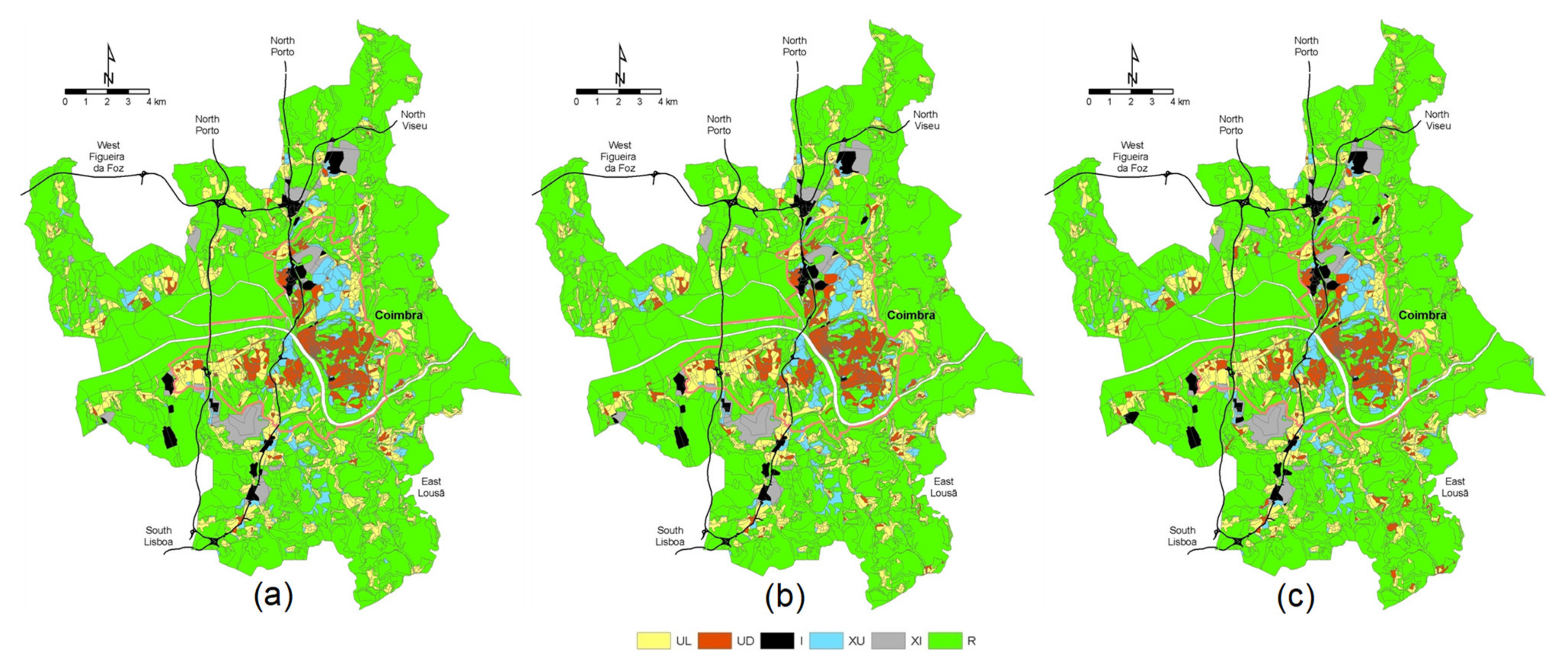
The model used the set of calibration parameters obtained from the calibration stage, with reference data to run forecast analysis for both scenarios starting from a reference situation in 2001 to the simulated map of 2021. It is possible to see the land use maps for the Baseline scenario for the two ten-year periods, with a starting reference situation in 2001 (Figure 6a) and simulation results for both 2011 (Figure 6b) and 2021 (Figure 6c). Likewise, land use maps for the simulation of the Anel scenario for the same years and starting from the same reference point of 2001 (Figure 7a) are depicted in Figure 7b for 2011 and in Figure 7c for 2021.
An overall analysis of these maps showed a spread distribution of land use change for urban land uses (UL and UH) across the main city of Coimbra and also the smaller settlements in both the urban and rural peripheries, especially in the Baseline scenario. However, the difference of the attractiveness of the region directly served by the new ring road for these urban land uses was also observable.
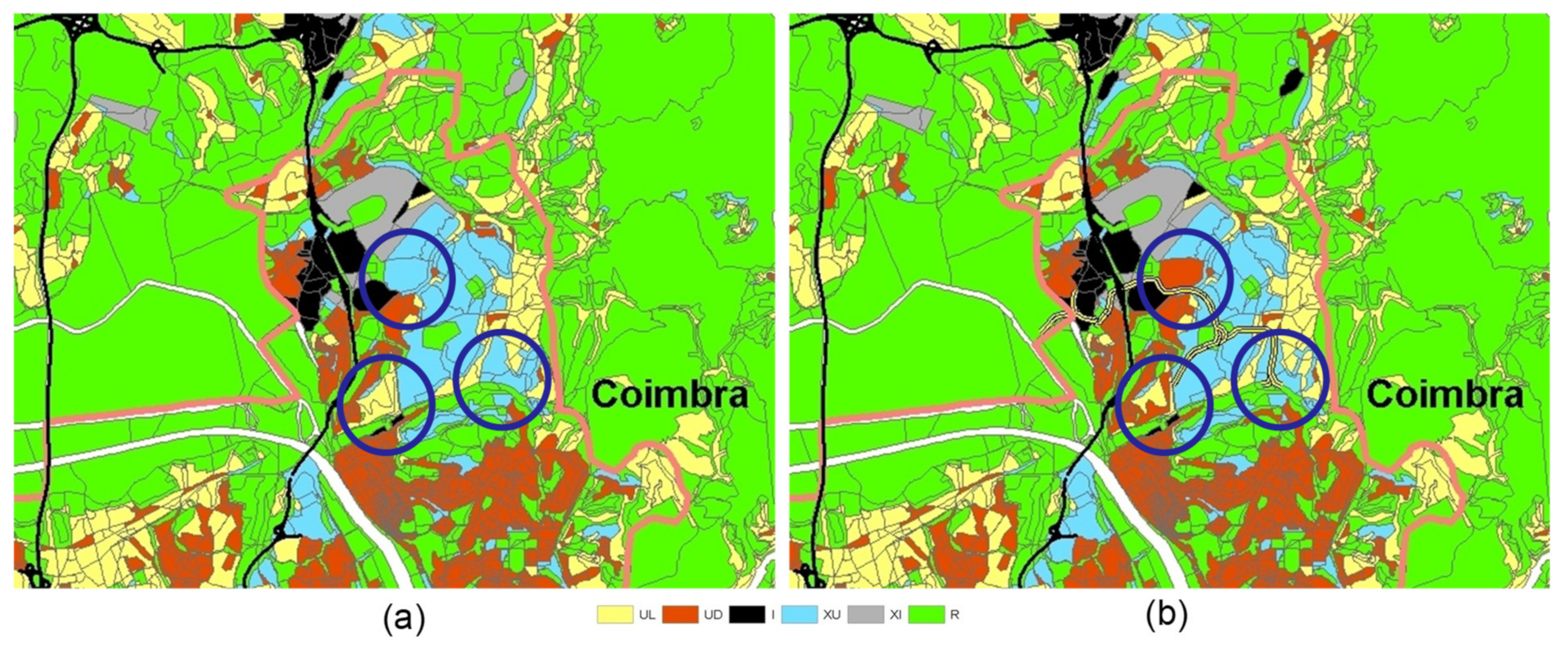
An enhanced detail of the area directly served by the new road is depicted in Figure 8a for the Baseline scenario and Figure 8b for the Anel scenario. These results show that the impact of the construction of the ring road was significant, as the higher attractiveness of cells directly served by the new road due to increased accessibility was well illustrated in the land use change in the Anel scenario, with more cells changing their states to more dense urban uses. This favoring of more dense urban uses followed what was considered in the planning documents to support the expansion of the northern area of the city of Coimbra, which was directly served by the ring road. The impact on the industrial land uses was less significant, as they were generally located at significant distances from the road and usually very close to the main collector roads, thus experiencing smaller increases in accessibility that benefited the central urban area more. The effect of neighborhood interaction (higher importance than accessibility) also played a significant role in this reduced attraction for industrial land uses in the area directly served by the ring road, which was mainly covered by urban (UL, UH and XU) land uses.
5. Conclusions
The model was applied to simulate the impact on urban growth of the construction of an important urban ring road in the city of Coimbra, Portugal. The main goal of this application was to illustrate the possibilities of using this type of modeling approach to capture and forecast the complex interactions between land use dynamics and changes in transport systems. The two scenarios designed for this application were quite simple, and they were meant to test the capacities of the model and not to support any planning process. Our model can be applied to similar case studies where irregular, vector-based cells can be used to model space, namely when the data and geography of census units are available at a resolution similar to that of our model. It can also be applied to multiple types of scenarios using the same data attributes as the ones presented in this article.
The results were useful for exemplifying what types of analysis could be made in order to support a discussion of different planning choices. These results were presented in a workshop about the application of land use and transport interaction models to both practitioners and elected officials of different backgrounds (spatial planning and transport planning) and different origins (local administration and governmental agencies). Although these scenarios were not designed for use in a real planning context, the results were useful for triggering a debate between modelers and potential users, who engage in preliminary discussions about strategic options in urban development.
There is great potential in using more complex transport models to provide better accessibility indicators to CA models. First, with the use of transport models and not just spatial measures (mainly distances), accessibility is no longer just an exogenous variable; it becomes a reliable measure of the performance of the transport system by (1) taking into account the effect of land use change on transport demand and (2) providing not only an input for the CA model, but also an effective lever to produce and evaluate changes in the transport system. Second, it is possible to relate land use parameters with transport parameters, testing different settings for their values in order to evaluate their interdependencies. This provides more robust tools to simulate the complexity of land use and transport interactions, enhancing the possibilities of performing policy testing with a combination of planning and transport policies and programs.
The results show that there is no particular barrier for coupling CA and transport models, other than some level of computational demand due to the increased number of calibration parameters. This can be solved by using calibration procedures based on optimization approaches that are able to deal with high numbers of parameters, such as the particle swarm algorithm. The literature on CA models already includes many models where transport and accessibility are modeled with more complex models. However, they use parallel procedures to calibrate these models and generate inputs to the CA model, and vice versa.
Future developments of this coupled application of CA-based land use models with accessibility modeling will take into account different aspects of the transport systems, namely service levels, different scales of analysis and multimodality, where variables such as pricing or new service areas can be simulated to understand the impact on land use change. At the same time, the CA model needs to incorporate procedures that trigger changes in the transport systems due to new demand, such as inducing the construction of new infrastructure or requiring a new transport service in a given mode.
Author Contributions
Conceptualization, Nuno Pinto, António P. Antunes and Josep Roca; data curation, Nuno Pinto; formal analysis, Nuno Pinto; funding acquisition, Nuno Pinto; investigation, Nuno Pinto; methodology, Nuno Pinto; project administration, Nuno Pinto; supervision, António P. Antunes and Josep Roca; visualization, Nuno Pinto; writing—original draft, Nuno Pinto; writing—review and editing, Nuno Pinto, António P. Antunes and Josep Roca. All authors have read and agreed to the published version of the manuscript.
Funding
This research was funded by the Fundação para a Ciência e Tecnologia (Portugal) under grant SFRH/BD/37465/2007.
Institutional Review Board Statement
Not applicable.
Informed Consent Statement
Not applicable.
Data Availability Statement
Publicly available datasets were analyzed in this study. This data can be found here: [www.ine.pt] and [http://bte.gep.mtsss.gov.pt/bteonline.php] (accessed on 30 December 2020).
Acknowledgments
The authors would like to thank the reviewers for their valuable comments.
Conflicts of Interest
The authors declare no conflict of interest.
References
- Alonso, W. Location and Land Use: Toward a General Theory of Land Rest; Harvard University Press: Cambridge, MA, USA, 1964; Volume 42, pp. 277–279. [Google Scholar]
- De la Barra, T. Integrated land use and transport modelling: The TRANUS experience. In Planning Support Systems: Integrating Geographical Information Systems, Models and Visualization Tools; Brail, R.K., Klosterman, R.E., Eds.; ESRI Press: Redlands, CA, USA, 2001; pp. 129–156. [Google Scholar]
- Halden, D. Using accessibility measures to integrate land use and transport policy in Edinburgh and the Lothians. Transp. Policy 2002, 9, 313–324. [Google Scholar] [CrossRef]
- Latuso, K. The SPARTACUS system for defining and analysing sustainable land use and transport policies. In Planning Support Systems in Practice; Geertman, S., Stillwell, J., Eds.; Springer: Heidelberg, Germany, 2003; pp. 453–463. [Google Scholar]
- Noth, M.; Borning, A.; Waddell, P. An extensible, modular architecture for simulating urban development, transportation, and environmental impacts. Comput. Environ. Urban Syst. 2003, 27, 181–203. [Google Scholar] [CrossRef]
- Neumann, J. The general and logical theory of automata. In Cerebral Mechanisms in Behavior; The Hixon Symposium; Taub, A.H., Ed.; Wiley: New York, NY, USA, 1951; pp. 1–41. [Google Scholar]
- Ulam, S.M. Some Ideas and Prospects in Biomathematics. Annu. Rev. Biophys. Bioeng 1972, 1, 277–292. [Google Scholar] [CrossRef] [PubMed]
- Benenson, I.; Torrens, P.M. Geosimulation—Automata-Based Modeling of Urban Phenomena, 1st ed.; John Wiley & Sons Ltd.: Chechester, UK, 2004; 287p. [Google Scholar]
- Tobler, W.R. Cellular Geography. In Philosophy in Geography; Gale, S., Olsson, G., Eds.; D. Reidel: Boston, MA, USA, 1979; pp. 379–386. [Google Scholar]
- Tobler, W.R. A Computer Movie Simulating Urban Growth in the Detroit Region. Econ. Geogr. 1970, 46, 234–240. [Google Scholar] [CrossRef]
- Aljoufie, M.; Zuidgeest, M.; Brussel, M.; van Vliet, J.; van Maarseveen, M. A cellular automata-based land use and transport interaction model applied to Jeddah, Saudi Arabia. Landsc. Urban. Plan. 2013, 112, 89–99. [Google Scholar] [CrossRef]
- Von Neumann, J. Theory of self-reproducing automata. In Information Storage and Retrieval; University of Illinois Press: Urbana, IL, USA, 1969; p. 403. [Google Scholar]
- Batty, M.; Xie, Y. From Cells to Cities. Environ. Plan. B Plan. Des. 1994, 21, S31–S48. [Google Scholar] [CrossRef]
- Couclelis, H. Cellular Worlds: A Framework for Modeling Micro—Macro Dynamics. Environ. Plan. A 1985, 17, 585–596. [Google Scholar] [CrossRef]
- Couclelis, H. Cellular dynamics: How individual decisions lead to global urban change. Eur. J. Oper. Res. 1987, 30, 344–346. [Google Scholar] [CrossRef]
- White, R.; Engelen, G. Cellular automata and fractal urban form: A cellular modelling approach to the evolution of urban land-use patterns. Environ. Plan. A 1993, 25, 1175–1199. [Google Scholar] [CrossRef] [Green Version]
- Barredo, J.; Kasanko, M. Modelling dynamic spatial processes: Simulation of urban future scenarios through cellular automata. Landsc. Urban. 2003, 64, 145–160. [Google Scholar] [CrossRef]
- Crols, T.; White, R.; Uljee, I.; Engelen, G.; Poelmans, L.; Canters, F. A travel time-based variable grid approach for an activity-based cellular automata model. Int. J. Geogr. Inf. Sci. 2015, 29, 1757–1781. [Google Scholar] [CrossRef] [Green Version]
- Liu, X.; Li, X.; Shi, X.; Wu, S.; Liu, T. Simulating complex urban development using kernel-based non-linear cellular automata. Ecol. Modell. 2008, 211, 169–181. [Google Scholar] [CrossRef]
- Silva, E.A.; Clarke, K.C. Complexity, emergence and cellular urban models: Lessons learned from applying sleuth to two Portuguese metropolitan areas. Eur. Plan. Stud. 2005, 13, 93–116. [Google Scholar] [CrossRef]
- Wu, F.; Webster, C.J. Simulation of land development through the integration of cellular automata and multicriteria evaluation. Environ. Plan. B Plan. Des. 1998, 25, 103–126. [Google Scholar] [CrossRef]
- Campos, P.B.R.; de Almeida, C.M.; de Queiroz, A.P. Educational infrastructure and its impact on urban land use change in a peri-urban area: A cellular-automata based approach. Land Use Policy. 2018, 79, 774–788. [Google Scholar] [CrossRef]
- Abolhasani, S.; Taleai, M.; Karimi, M.; Rezaee Node, A. Simulating urban growth under planning policies through parcel-based cellular automata (ParCA) model. Int. J. Geogr. Inf. Sci. 2016, 30, 2276–2301. [Google Scholar] [CrossRef]
- Barreira-González, P.; Gómez-Delgado, M.; Aguilera-Benavente, F. From raster to vector cellular automata models: A new approach to simulate urban growth with the help of graph theory. Comput. Environ. Urban. Syst. 2015, 54, 119–131. [Google Scholar] [CrossRef]
- Barreira-González, P.; Barros, J. Configuring the neighbourhood effect in irregular cellular automata based models. Int. J. Geogr. Inf. Sci. 2017, 31, 617–636. [Google Scholar] [CrossRef]
- Moreno, N.; Ménard, A.; Marceau, D.J. VecGCA: A vector-based geographic cellular automata model allowing geometric transformations of objects. Environ. Plan. B Plan. Des. 2008, 35, 647–665. [Google Scholar] [CrossRef] [Green Version]
- Moreno, N.; Wang, F.; Marceau, D.J. Implementation of a dynamic neighborhood in a land-use vector-based cellular automata model. Comput. Environ. Urban Syst. 2009, 33, 44–54. [Google Scholar] [CrossRef]
- O’Sullivan, D. Exploring spatial process dynamics using irregular graph-based cellular automaton models. Geogr. Anal. 2001, 33, 1–18. [Google Scholar] [CrossRef]
- Semboloni, F. The growth of an urban cluster into a dynamic self-modifying spatial pattern. Environ. Plan. B Plan. Des. 2000, 27, 549–564. [Google Scholar] [CrossRef]
- Stevens, D.; Dragicevic, S.; Rothley, K. iCity: A GIS-CA modelling tool for urban planning and decision making. Environ. Model Softw. 2007, 22, 761–773. [Google Scholar] [CrossRef]
- Wang, F.; Marceau, D.J. A Patch-based Cellular Automaton for Simulating Land-use Changes at Fine Spatial Resolution. Trans. Gis. 2013, 17, 828–846. [Google Scholar] [CrossRef]
- Zhu, J.; Sun, Y.; Song, S.; Yang, J.; Ding, H. Cellular automata for simulating land-use change with a constrained irregular space representation: A case study in Nanjing city, China. Environ. Plan. B Urban. Anal. City Sci. 2020, 1–19. [Google Scholar]
- Chen, Y.; Liu, X.; Li, X. Calibrating a Land Parcel Cellular Automaton (LP-CA) for urban growth simulation based on ensemble learning. Int. J. Geogr. Inf. Sci. 2017, 31, 2480–2504. [Google Scholar] [CrossRef]
- Antunes, A.; Seco, Á.; Pinto, N. An accessibility-maximization approach to road network planning. Comput. Civ. Infrastruct. Eng. 2003, 18, 224–240. [Google Scholar] [CrossRef]
- Dalvi, M.Q. Behavioural modelling, accessibility, mobility and need: Concepts and measurement. In Behavioural Travel Modelling; Croom Helm: London, UK, 1978; pp. 639–653. [Google Scholar]
- Bhat, C.R.; Handy, S.L.; Kockelman, K.M.; Mahmassani, M.; Chen, Q.; Weston, L. Development of an Urban Accessibility Index: Literature Review. 2000. Available online: https://trid.trb.org/view/719047 (accessed on 30 December 2020).
- Bertolini, L.; le Clercq, F.; Kapoen, L. Sustainable accessibility: A conceptual framework to integrate transport and land use plan-making. Two test-applications in the Netherlands and a reflection on the way forward. Transp. Policy 2005, 12, 207–220. [Google Scholar] [CrossRef]
- CURR. Mandebus—Manchester Decision Based Urban Simulator: Final Report to SSRC. Results from a Single Zone Model; Centre for Urban and Regional Research, University of Manchester: Manchester, UK, 1981; unpublished work. [Google Scholar]
- Waddell, P. Between politics and planning: UrbanSim as a decision-support system for metropolitan planning. In Planning Support Systems: Integrating Geographical Information Systems, Models and Visualization Tools; Brail, R.K., Klosterman, R.E., Eds.; ESRI Press: Redlands, CA, USA, 2001; pp. 201–228. [Google Scholar]
- Santé, I.; García, A.M.; Miranda, D.; Crecente, R. Cellular automata models for the simulation of real-world urban processes: A review and analysis. Landsc. Urban. Plan. 2010, 96, 108–122. [Google Scholar] [CrossRef]
- Basse, R.M. A constrained cellular automata model to simulate the potential effects of high-speed train stations on land-use dynamics in trans-border regions. J. Transp. Geogr. 2013, 32, 23–37. [Google Scholar] [CrossRef]
- Clarke, K.C.; Hoppen, S.; Gaydos, L. A self-modifying cellular automaton model of historical urbanization in the San Francisco Bay area. Environ. Plan. B Plan. Des. 1997, 24, 247–261. [Google Scholar] [CrossRef] [Green Version]
- He, C.; Okada, N.; Zhang, Q.; Shi, P.; Li, J. Modelling dynamic urban expansion processes incorporating a potential model with cellular automata. Landsc. Urban Plan. 2008, 86, 79–91. [Google Scholar] [CrossRef]
- Li, X.; Yeh, A.G.O. Modelling sustainable urban development by the integration of constrained cellular automata and GIS. Int. J. Geogr. Inf. Sci. 2000, 14, 131–152. [Google Scholar] [CrossRef]
- Sakieh, Y.; Salmanmahiny, A.; Jafarnezhad, J.; Mehri, A.; Kamyab, H.; Galdavi, S. Evaluating the strategy of decentralized urban land-use planning in a developing region. Land Use Policy 2015, 48, 534–551. [Google Scholar] [CrossRef]
- Yang, Q.S.; Li, X.; Shi, X. Cellular automata for simulating land use changes based on support vector machines. Comput. Geosci. 2008, 34, 592–602. [Google Scholar] [CrossRef]
- Navarro Cerrillo, R.M.; Palacios Rodríguez, G.; Clavero Rumbao, I.; Lara, M.Á.; Bonet, F.J.; Mesas-Carrascosa, F.-J. Modeling Major Rural Land-Use Changes Using the GIS-Based Cellular Automata Metronamica Model: The Case of Andalusia (Southern Spain). ISPRS Int. J. Geo-Inf. 2020, 9, 458. [Google Scholar] [CrossRef]
- Zhao, L.; Shen, L. The impacts of rail transit on future urban land use development: A case study in Wuhan, China. Transp. Policy 2019, 81, 396–405. [Google Scholar] [CrossRef]
- RIKS. Metronamica. Maastricht, The Netherlands. 2015. Available online: http://www.metronamica.nl/ (accessed on 30 December 2020).
- Zhao, L.; Peng, Z.R. LandSys: An agent-based Cellular Automata model of land use change developed for transportation analysis. J. Transp. Geogr. 2012, 25, 35–49. [Google Scholar] [CrossRef]
- Couto, P. Assessing the accuracy of spatial simulation models. Ecol. Modell. 2003, 167, 181–198. [Google Scholar] [CrossRef]
- Cohen, J. A coeficient of agreement for nominals scales. J. Educ. Meas. 1960, 20, 37–46. [Google Scholar] [CrossRef]
- Congalton, R.G.; Green, K. Assessing the Accuracy of Remotely Sensed Data: Principles and Practices. The Photogrammetric Record; Wiley: New York, NY, USA, 2009; Volume 2, 183p. Available online: http://www.loc.gov/catdir/enhancements/fy0744/98029658-d.html (accessed on 30 December 2020).
- Pontius, R.G.; Millones, M. Death to Kappa: Birth of quantity disagreement and allocation disagreement for accuracy assessment. Int. J. Remote Sens. 2011, 32, 4407–4429. [Google Scholar] [CrossRef]
- Kang, J.; Fang, L.; Li, S.; Wang, X. Parallel Cellular Automata Markov Model for Land Use Change Prediction over MapReduce Framework. ISPRS Int. J. Geo-Inf. 2019, 8, 454. [Google Scholar] [CrossRef] [Green Version]
- Grinblat, Y.; Gilichinsky, M.; Benenson, I. Cellular Automata Modeling of Land-Use/Land-Cover Dynamics: Questioning the Reliability of Data Sources and Classification Methods. Ann. Am. Assoc. Geogr. 2016, 106, 1299–1320. [Google Scholar] [CrossRef]
- Petrov, L.O.; Lavalle, C.; Kasanko, M. Urban land use scenarios for a tourist region in Europe: Applying the MOLAND model to Algarve, Portugal. Landsc. Urban Plan. 2009, 92, 10–23. [Google Scholar] [CrossRef]
- Van Vliet, J.; Bregt, A.K.; Hagen-Zanker, A. Revisiting Kappa to account for change in the accuracy assessment of land-use change models. Ecol. Modell. 2011, 222, 1367–1375. [Google Scholar] [CrossRef]
- Pinto, N.N.; Antunes, A.P. A cellular automata model based on irregular cells: Application to small urban areas. Environ. Plan. B Plan. Des. 2010, 37, 1095–1114. [Google Scholar] [CrossRef]
- Eberhart, R.; Kennedy, J. A new optimizer using particle swarm theory. In MHS’95 Proceedings of the Sixth International Symposium on Micro Machine and Human Science; IEEE: New York, NY, USA, 1995; pp. 39–43. Available online: http://0-ieeexplore-ieee-org.brum.beds.ac.uk/document/494215/ (accessed on 30 December 2020).
- Parsopoulos, K. Recent approaches to global optimization problems through particle swarm optimization. Nat. Comput. 2002, 1, 235–306. [Google Scholar] [CrossRef]
- Pinto, N.; Antunes, A.P.; Roca, J. Applicability and calibration of an irregular cellular automata model for land use change. Comput. Environ. Urban Syst. 2017, 65, 93–102. [Google Scholar] [CrossRef] [Green Version]
- Feng, Y.; Liu, Y.; Tong, X.; Liu, M.; Deng, S. Modeling dynamic urban growth using cellular automata and particle swarm optimization rules. Landsc. Urban Plan. 2011, 102, 188–196. [Google Scholar] [CrossRef]
- Liao, J.; Tang, L.; Shao, G.; Qiu, Q.; Wang, C.; Zheng, S.; Su, X. A neighbor decay cellular automata approach for simulating urban expansion based on particle swarm intelligence. Int. J. Geogr. Inf. Sci. 2014, 28, 720–738. [Google Scholar] [CrossRef]
- INE. As Cidades em Números. 1.0; Instituto Nacional de Estatística: Lisbon, Portugal, 2004. [Google Scholar]
- INE. Censos 2001. 1.0; Instituto Nacional de Estatística: Lisbon, Portugal, 2001; Available online: http://www.ine.pt (accessed on 30 December 2020).
- GEP. Boletim do Trabalho e Emprego. Available online: http://bte.gep.mtsss.gov.pt/bteonline.php (accessed on 30 December 2020).
- Xiang, W.N.; Clarke, K.C. The use of scenarios in land-use planning. Environ. Plan. B Plan. Des. 2003, 30, 885–909. [Google Scholar] [CrossRef] [Green Version]
Figure 1.
Two examples of neighborhood effect interactions between pairs of cell states: (a) attraction), (b) repulsion.
Figure 1.
Two examples of neighborhood effect interactions between pairs of cell states: (a) attraction), (b) repulsion.

Figure 2.
Calibration flowchart with the particle swarm (PS) structure encapsulating the cellular automata (CA) model.
Figure 2.
Calibration flowchart with the particle swarm (PS) structure encapsulating the cellular automata (CA) model.

Figure 3.
Location of the municipality of Coimbra, Portugal.
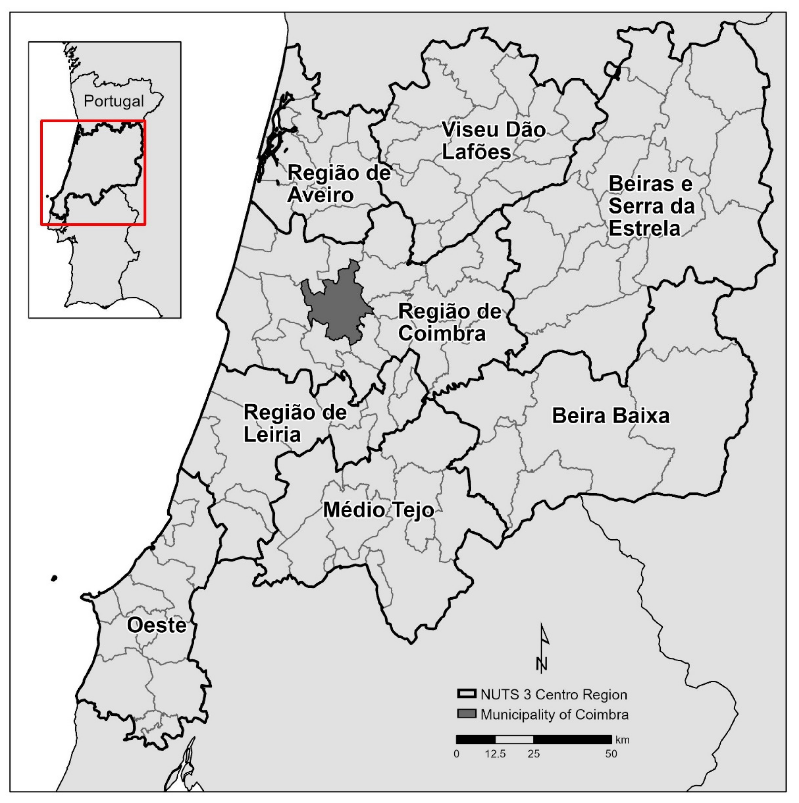
Figure 4.
Land use maps for the municipality of Coimbra, with references for (a) 1991 and (b) 2001, as well as (c) the simulation results for 2001.
Figure 4.
Land use maps for the municipality of Coimbra, with references for (a) 1991 and (b) 2001, as well as (c) the simulation results for 2001.
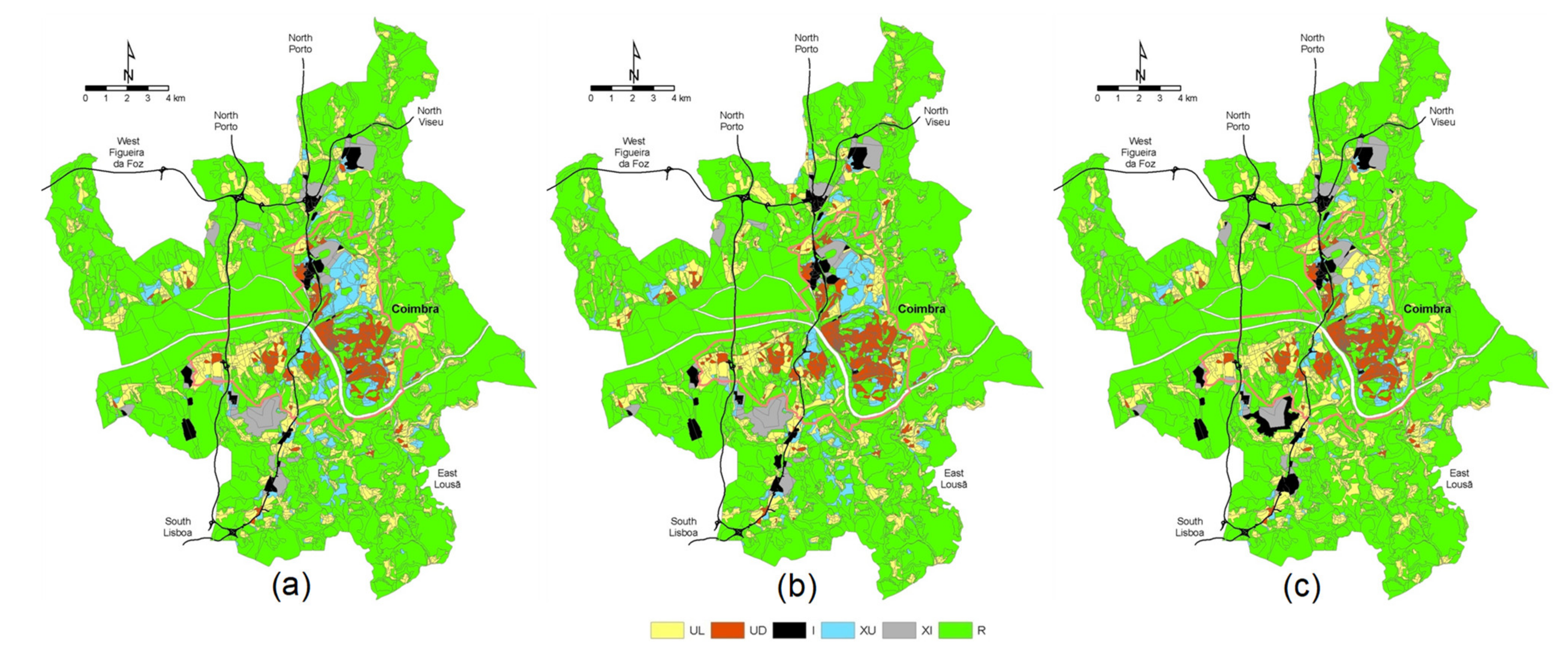
Figure 5.
Road network of the municipality of Coimbra in 2021 for (a) the Baseline scenario and (b) the Anel scenario.
Figure 5.
Road network of the municipality of Coimbra in 2021 for (a) the Baseline scenario and (b) the Anel scenario.
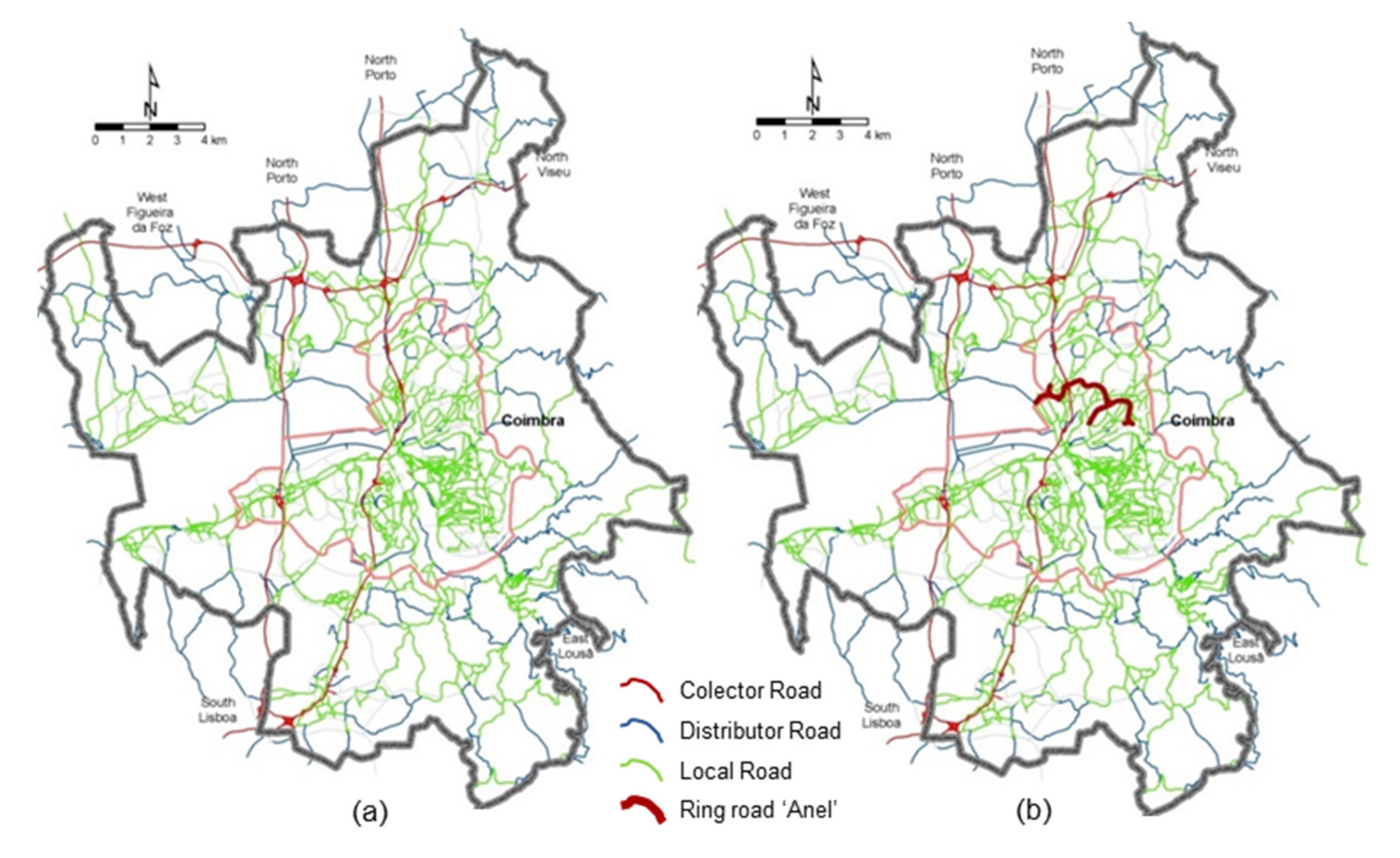
Figure 6.
Land use maps for the municipality of Coimbra in the Baseline scenario, showing (a) a reference for 2001 and simulations for (b) 2011 and (c) 2021.
Figure 6.
Land use maps for the municipality of Coimbra in the Baseline scenario, showing (a) a reference for 2001 and simulations for (b) 2011 and (c) 2021.
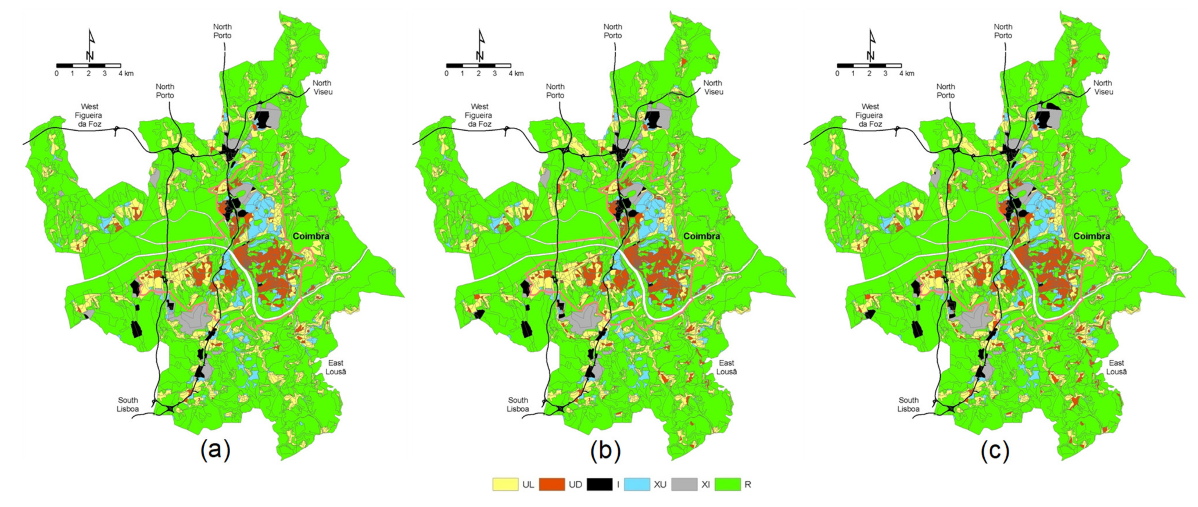
Figure 7.
Land use maps for the municipality of Coimbra in the Anel scenario, showing (a) a reference for 2001 and simulations for (b) 2011 and (c) 2021.
Figure 7.
Land use maps for the municipality of Coimbra in the Anel scenario, showing (a) a reference for 2001 and simulations for (b) 2011 and (c) 2021.

Figure 8.
Land use maps for the area directly served by the new ring road in (a) the Baseline scenario and (b) the Anel scenario.
Figure 8.
Land use maps for the area directly served by the new ring road in (a) the Baseline scenario and (b) the Anel scenario.


Table 1.
Macro-indicators for population and employment growth for both scenarios.
| 2001–2011 | 2011–2021 | |
|---|---|---|
| Population | +3% | +2% |
| Employment | +2% | +2% |
Publisher’s Note: MDPI stays neutral with regard to jurisdictional claims in published maps and institutional affiliations. |
© 2021 by the authors. Licensee MDPI, Basel, Switzerland. This article is an open access article distributed under the terms and conditions of the Creative Commons Attribution (CC BY) license (http://creativecommons.org/licenses/by/4.0/).
Share and Cite
MDPI and ACS Style
Pinto, N.; Antunes, A.P.; Roca, J. A Cellular Automata Model for Integrated Simulation of Land Use and Transport Interactions. ISPRS Int. J. Geo-Inf. 2021, 10, 149. https://0-doi-org.brum.beds.ac.uk/10.3390/ijgi10030149
AMA Style
Pinto N, Antunes AP, Roca J. A Cellular Automata Model for Integrated Simulation of Land Use and Transport Interactions. ISPRS International Journal of Geo-Information. 2021; 10(3):149. https://0-doi-org.brum.beds.ac.uk/10.3390/ijgi10030149
Chicago/Turabian StylePinto, Nuno, António P. Antunes, and Josep Roca. 2021. "A Cellular Automata Model for Integrated Simulation of Land Use and Transport Interactions" ISPRS International Journal of Geo-Information 10, no. 3: 149. https://0-doi-org.brum.beds.ac.uk/10.3390/ijgi10030149
Note that from the first issue of 2016, this journal uses article numbers instead of page numbers. See further details here.