
A Century of French Railways: The Value of Remote Sensing and VGI in the Fusion of Historical Data


CNRS UMR 8049 LIGM, Université Gustave-Eiffel, Cité Descartes, 5 Descartes, 77454 Marne-la-Vallée, France
ISPRS Int. J. Geo-Inf. 2021, 10(3), 154; https://0-doi-org.brum.beds.ac.uk/10.3390/ijgi10030154
Submission received: 27 December 2020
/
Revised: 2 March 2021
/
Accepted: 6 March 2021
/
Published: 10 March 2021
Abstract
:Providing long-term data about the evolution of railway networks in Europe may help us understand how European Union (EU) member states behave in the long-term, and how they can comply with present EU recommendations. This paper proposes a methodology for collecting data about railway stations, at the maximal extent of the French railway network, a century ago.The expected outcome is a geocoded dataset of French railway stations (gares), which: (a) links gares to each other, (b) links gares with French communes, the basic administrative level for statistical information. Present stations are well documented in public data, but thousands of past stations are sparsely recorded, not geocoded, and often ignored, except in volunteer geographic information (VGI), either collaboratively through Wikipedia or individually. VGI is very valuable in keeping track of that heritage, and remote sensing, including aerial photography is often the last chance to obtain precise locations. The approach is a series of steps: (1) meta-analysis of the public datasets, (2) three-steps fusion: measure-decision-combination, between public datasets, (3) computer-assisted geocoding for ‘gares’ where fusion fails, (4) integration of additional gares gathered from VGI, (5) automated quality control, indicating where quality is questionable. These five families of methods, form a comprehensive computer-assisted reconstruction process (CARP), which constitutes the core of this paper. The outcome is a reliable dataset—in geojson format under open license—encompassing (by January 2021) more than 10,700 items linked to about 7500 of the 35,500 communes of France: that is 60% more than recorded before. This work demonstrates: (a) it is possible to reconstruct transport data from the past, at a national scale; (b) the value of remote sensing and of VGI is considerable in completing public sources from an historical perspective; (c) data quality can be monitored all along the process and (d) the geocoded outcome is ready for a large variety of further studies with statistical data (demography, density, space coverage, CO2 simulation, environmental policies, etc.).
1. Introduction
Transport infrastructure for people and goods is as old as urban civilizations, e.g., Via Appia, Aemilia, Aurelia, etc. have helped in structuring the European landscape for centuries. From 1920 to 2020, the evolution of road and rail networks is a well known element of their competition [1,2,3]. Today climate challenges reignite that century-old debate:for instance the European Union (EU) transportation white paper [4] notes that in 2010 rail yielded11 million tons of CO2, versus road: 191 m tons, but regrets “… that only limited data are available …” for measuring the impact of measures by member states. Linking railway data with socio-eco-demographic data in historical geographic information systems (GIS), would contribute to understanding long-term trends. This approach has been developed by Siebert [5], and, in Europe by Gregory et al. [6], and Morillas-Torné [7] with a very similar goal, and uses several European public datasets, which record main rail lines (no secondary rail lines).
This paper describes a method for building a digital representation of all the ‘stations’ (we use the French term ‘gare’) that have existed, between the maximum extent of the French railway network (1920s) and now, a century later. The goal is to deliver a dataset to answer questions such as: Does a commune possesses a gare? How far from the closest gare? Also, the aim is to give a comparison at different dates. For that we need: (a) to link gares to each other along their ‘rail line’ (we use French term ‘ligne’), (b) to link every gare to a ‘city or town’: we use the French term ‘commune’, the smallest French administrative level at which most basic statistical data are collected.
There is no digital dataset providing all French gares at the maximum extent of the network, and even their number is unknown. There are two kinds of source: public records (open data from French public institutions: SNCF, Insee, IGN over 2014–2020), and a lot of volunteered geographic information (VGI), either collective through Wikipedia, or individual, providing sparse data about old gares (even simple stops) and lignes.
Section 2 and Section 3 present materials and methods, respectively for public and VGI sources, with the goal to “geocode” all the gares, in a reliable, controllable way; as “points-of-interest” multi-source matching is presented in Li et al. [8].
Multi-source datasets are expected to show discrepancies between names (toponym changes), as investigated by Tian-Lan and Longley [9], and locations (existence and geocoding) of each individual gare. In order to resolve discrepancies, target constraints are formulated, and a schema is proposed. Each source is scrutinized by a “meta-analysis” [10,11], in order to identify what may conflict the constraints. Then public datasets are inputted in a fusion process, following Bloch [12], which more precisely is an asymmetric revision, as in Benferhat et al. [13], in a background similar to Reichgelt [14].
Issues raised by VGI have been addressed, e.g., by Johnson and Iizuka [15] successfully combining OpenStreetMap features and Landsat image classification; by Younghoon et al. [16] integrating several crowdsourcing sets in a single graph,or possibly developing collaborative platform such as FeatureHub [17]; or multiple platforms as in Juhász et al. [18]. The specific goal assigned to VGI in this paper is to gather data for revising some already geocoded gares (whose quality is questioned), and mostly for integrating more gares, not recorded in public datasets. Chen et al. [19] have developed CrowdFusion, a framework aiming at data refinement (a hard non-polynomial task), while Gouvëa et al. [20], and Hastings [21], have focused on toponym conflation and gazetteer-based geo-referencing.
Section 3 describes routines querying Wikipedia for coordinates of gares, and mostly to parsing railway-oriented “Infobox” [22]. There are some inspiringpapers about how to populatethem [23], or to extract information based on common-sense rules [24]. An Infobox is a very valuable means to obtain at once the information about a ligne, the other lignes it connects with, and the gares it encompasses. The parsing of the information that complies with target constraints is one important contribution of the present work, because, beyond French peculiarities, railway semantics is shared by most countries. Next, Section 3 describes several ways in querying various VGI sources, mostly about gares on secondary lignes (e.g., the popular rural tramways in France, between WWI and WWII). The last opportunity to resolve failed geocoding issues, is to exploit remote-sensing images, old aerial photographs, and contemporary or 20th-century maps.
Issues of enacting data quality within a data collection process have been addressed by Vasseur et al. [25], who evaluates the quality in the context of a target use, and [26,27], two reviews about quality control in crowdsourcing, by Daniel et al. and Senaratne et al.
The mix of manual and software steps presented above, combines into what we name the computer-assisted reconstruction procedure (CARP). Finally, the resulting CARP dataset is cleaned up by an assisted data quality control.
2. Materials and Methods. Part 1: Public Data, Revision and Control
2.1. Shaping the Expected Target
2.1.1. Target Goal, Constraints and Initial Schema
The target should allow us to answer questions such as:
- -
- For each of the French communes, how far from its center is the closest gare?
- -
- Between closest garesof communes A and B, what is the closest path (kilometers)?
- -
- Comparing today and a century ago.
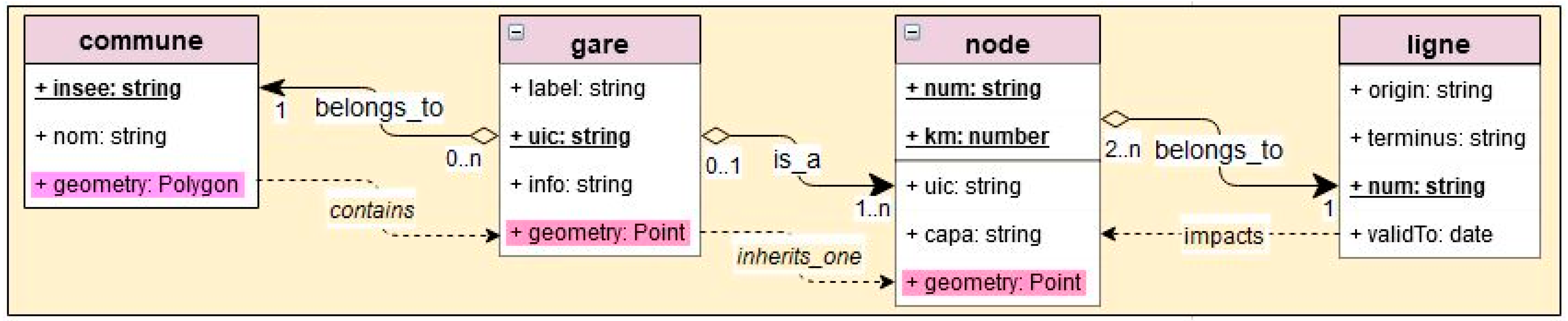
For that purpose, we need the minimal information to linking gares with communes, and to linking gares with lignes. That minimal information can be aligned with some components of the standards for transportation networks developed by the European infrastructure INSPIRE [28] or the Open geographic consortium OGC [29]. Four classes seem the minimum required: gare, commune, ligne, and a node class that allows one gare to be attached to several lignes (a “junction” gare).
The UML-class diagram (Figure 1) illustrates the relationships and their cardinalities, between these classes, and some additional constraints.
The “belongs_to” relationships of Figure 1, are very important:
- The gare–commune relationship is straightforward, once all gares are geocoded;
- The gare–ligne relationship is the challenge: how to find old lignes and all their gares.
Additional spatial constraint (contains) controls that a gare ‘belongs_to’ a commune, and (inherits_one) states that at least one node gives its coordinates to the gare (what about the other ones, if any? This is anissue studied in the sequel).
Some target concepts matching some INSPIRE ones (Figure 2), e.g.,
- -
- node → RailwayNode || RailwayStationNode;
- -
- gare → [RailwayNode(West), RailwayStationNode, RailwayNode(East)];
- -
- km (point kilométrique) → linear referencing,
- -
- uic (Union Internationale des Chemins de fer, the Worldwide Railway Organization (UIC) code) → RailwayStationCode, etc.
2.1.2. Target Attributes for Classes Commune, Gare, Ligne
Main attributes (mandatory) are:
- -
- insee = [primary key] official unique code for a commune, (may evolve with time);
- -
- num = [primary key] official number for a ligne, or any given unique code.;
- -
- uic = [primary key] official RailwayStationCodefor a gare, given by the UIC, the international railway organization, or any given unique code;
- -
- km = linear referencing, French:”point kilométrique”, German: “Streckenkilometer”;
- -
- the couple (num, km) is [primary key] for a gare (not two equal km for one num);
Geographical attributes (mandatory):
- -
- point = geocode of a node, and for the associated gare;
- -
- polygon = contour of a commune;
- -
- geometry in the sequel, is used to denote either point, or polygon.
Time attributes (mandatory, only one by now):
- -
- validTo = year of end of service of a ligne (hence of all its gares). A ligne can be disused partly (% of full length) at different dates, definitively (French: déclassement) or reversibly. Most recent year is used (INSPIRE: validTo).
Additional attributes (useful for display purposes, quality control):
- -
- label = name given to a gare (should be in bijection with uic) or a node;
- -
- nom = toponym for a commune (when used for a gare, may differ from the label);
- -
- capa = use status, e.g., ‘cargo only’, ‘border point’, etc. used for display purposes.
Summing up the constraints that must be satisfied:
- (1).
- (2).
- A couple (num, km) must be unique;
- (3).
- A couple (num, label), must be unique (see Section 2.3.1 and Appendix B);
- (4).
- The subset of all nodes of a same ligne (= num) must be strictly ordered by km;
- (5).
- Every gare belongs to one commune, whose polygon contains the garepoint. Sometimes, purposely, a gare has been built at the border of two communes (only one is recorded);
- (6).
- Every ligne has two ends: an origin node, and a terminus node. One ligne either is “active”, or has a “validTo” (alias “end”) date;
- (7).
- Every gare has one or more node(s), but a node may have no gare (e.g., a fork);
Constraints (1–4) are checked a priori (go/no-go), also a posteriori for quality control.
Constraint (5) can be checked a posteriori, setting, or controlling the insee value.
Constraint (6): a failure must trigger a search for additional information (Section 3).
Constraint (7): several nodes attached to the same gare, may differ in geometry, what is a major cause of indecision in the fusion process.
2.1.3. Target Notation and Generic Step-by-Step Approach for Collecting Values
The overall objective is to gather as many gares as possible that have ever existed. Therefore, the process starts with an initial dataset, then grow it, in a logical consistent way, by adding complementary or supplementary information from more available data.
To add a gare, means to create a node and to fill in attribute data step by step (Table 1), starting with the knowledge that a gare named label belongs to the ligne identified by num. In general, information about a ligne contains a list of the gares in between origin and terminus, which allows to set km values in correct order, although approximate in kilometers.
Attribute uic, is either given and the node is linked to this gare, or derived from (num, km).
Attribute insee, is either given or derived from geometry of gare and,commune.
Attributes capa, info are merely informative (voidable).
The baseline goal is to build a dataset, compliant with the above target constraints.
Constraints are flexible enough for semi-structured VGI (Section 3), while allowing consistency checking at every stage, for every source, and for the result as well.
Connectivity is not explicit in that model, but can be retrieved from the existence of several couples (num, uic) for a same uic, which denotes a “junction-gare”, or by the explicit identification of a fork between 2 lignes (see Discussion and Appendix B).
2.2. Public Open Data Sources, and the Information Revision Problem
In a project it is customary to define a baseline, which encompasses: goal, constraints (listed above), resources (listed below), estimated cost (time to target goal).
Baseline resources are versions (2020, 2017, 2014) of a public datasets originating from SNCF-Réseau (French national operator) [30], somewhat similar to the target schema.
Baseline cost is the cost per gare times the number of expected gares. The cost for one gare, depends on the steps outlined in Table 1. The number of expected gares, has not been found in the literature: for instance Auphan [31] estimates the maximum length of the network at 70,000 km in 1920, but does notmention a number of gares or communes impacted at that time. An estimation can use length and density of the network, e.g., 24,000 km today, serving 3029 “gares du réseau français” [32], gives a gare every 7.92 km. That inter-gare distance was lower in 1920, with stops in every crossed commune: a sampling on already reconstructed data gives about 6 km. Therefore, the number can be up to 12,000 gares.
2.2.1. Description of the Available Public and Administrative Sources
2.2.2. Matching Attributes of the Public Sources with Target Attributes
Among the attributes, there are some direct, or some indirect matches:
- Target.num: matches SNCF*|Lignes:code_ligne, primary key for lignes. Mandatory;
- Target.label: matches SNCF1:nom, and SNCF2*:libelle;
- Target.km: matches SNCF2*:pk. Mandatory. Order must reflect the strict order of the nodes on the ligne;
- Target.uic: matches SNCF2*:code_uic. In SNCF1, uses Target.label instead;
- couples SNCF1:(code_ligne, nom) and SNCF2:(code_ligne, pk), are used as primary key for nodes what requires to check its uniqueness;
- Target.capa: derived from SNCF:nature, SNCF*:fret,voyageurs or Lignes:mnemo, whichever available;
- Target.geometry: matches SNCF1:(latitude,longitude), SNCF2*:geometry:point,
- Target.insee: present in Insee-geo or Insee-new datasets, is primary key for communes, and must be retrieved for a gare, by identifying which commune verifies Point_in_Polygon(geometry(gare), geometry(commune));
- Target.nom: matches SNCF2:commune, would rather be retrieved via Target.insee;
2.3. Meta-Analysis of Public Sources, Building a Similarity Measure, and Corrections
The various Sncf versions provide scarce metadata [28], only about their lineage: how to check if a dataset complies with the target constraints? the only way is to perform a “meta-analysis”, a technique using “individual participant data” (IPD-MA), mainly developed in medicine [9,10].
The math behind meta-analysis uses variance-covariance matrices. In this application, “individual participants” are nodes of gares, and data are qualitative: hence, only equality can be checked, leading to true/false values. Therefore mathematics boils down to simple counts of items sharing equal attribute values. The meta-analysis is applied directly on the individual items of each dataset, and proves useful in the subsequent fusion.
Counting single attribute occurrences performs anunivariate meta-analysis, counting joint occurrences by a couple of attributes performs a multivariate meta-analysis.
This subsection is devoted to detailing what issues are revealed by the meta-analysis, helping to design the steps of a fusion approach. For aquick read, skip directly to Section 2.4 to discover the fusion, and return later to understanding the reasons why.
2.3.1. Meta-Analysis of Each Dataset, and Comparison
This is performed by the metaAnalysis routine (Appendix A).
- Step 1: univariate meta-analysis with num and label values. Result: each node has a num and a label value, in both 2014 and 2017, what fulfills the target first requirement. All 6442 nodes have a geometry in 2014, but only 6812 nodes have a geometry in 2017.
- Step 2: multivariate meta-analysis with uic, label, and (uic-label) values: 2017 only.
There are 6813 different label, but 6817 different (uic-label) values, what means that 4 couples (=label, ≠uic) are denoting a toponym ambiguity, e.g.,: "Cernay". Ambiguity is inherent to toponymy (in most countries): this is a well known issue [20,21]. Several mismatching examples and an explanation are proposed in Appendix B for what is named the “toponym-pattern”.
- Step 3: multivariate meta-analysis with (label-num) and (uic-num) couples
In both 2014 and 2017, 6 nodes have equal values (=label, =num) or (=uic, =num), meaning data duplication e.g.,“Saintes” (cf. routine disDuplicate in Appendix A).
- Step 4: inspect the geometry of Step3 couples: if a same label or uic occurs in several nodes, it denotes a junction-gare (=uic, ≠num). Associated geometryare expected to be equal: the computed deviation is broken down into five distance intervals (Table 4).
The choice of the values (150 m, 300 m, 1 km, 2 km) is explained in Section 2.4.
In 2014, among 642 nodes, 93% are “close enough”, and 1% “rather far”. For instance, above 2 km, the “Bauvin-Provin” case, is named a “fork-pattern”, for the closure of a ligne has “moved” the node to a remote location at the last fork on that ligne. An analysis of the “fork-pattern” is proposed in Appendix B.
In 2017, among 1360 nodes, 53% are “close enough”, but 635 are not (47%). The cause of so many discrepancies is that more “fork-patterns” are taken into account in 2017.
It’s impossible to choose the right geometry without extra information, moreover, the wrong location is not an error, but a meaningful node: the solution is to mark it (Section 2.4).
- Step 5: inspect the cardinal of Step3 couples, for every num value: thisgives the number of nodes per ligne (Table 5).
A ligne with one gare denotes an “isolated” gare, which is a conflicting constraint. Most of these errors correspond to lignes now closed to traffic (fork-pattern again), which requires extra information, not available at that stage.
2.3.2. Conclusion of the Meta-Analysis
The meta-analysis has been applied to the two main public datasets providing gare information: the result is a better understanding of what data must be handled, which helps designing a fusion approach to merging data from 2014 and 2017. In particular, it helps in understanding that the “toponymy-patter” and the “fork-pattern” constitute hurdles in the fusion process, and will require additional information from external VGI sources.
The meta-analysis can be used as a quality control tool at any time at any stage of the reconstruction process, and will be used to control the result (Section 4).
The outcome of the meta-analysis of the initial datasets, is that 890 nodes are not geocoded, and 635 otherhave a poor geometry (Table 4), and would rather be avoided in the fusion process.
2.4. Combining the Available Sources: The Fusion/Revision Problem
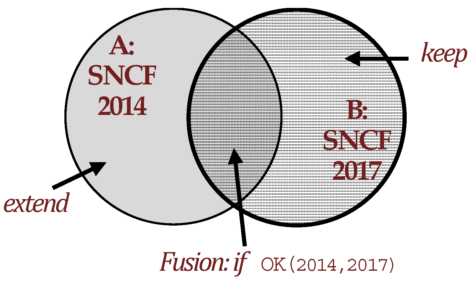
Versions Sncf2014 and Sncf2014 probably have a same origin, then evolved separately. Sncf2017 has more attributes, notably the km, and uic, and a few more geocoded features (6812 versus 6442) although we do notknow which version would provide the best quality.
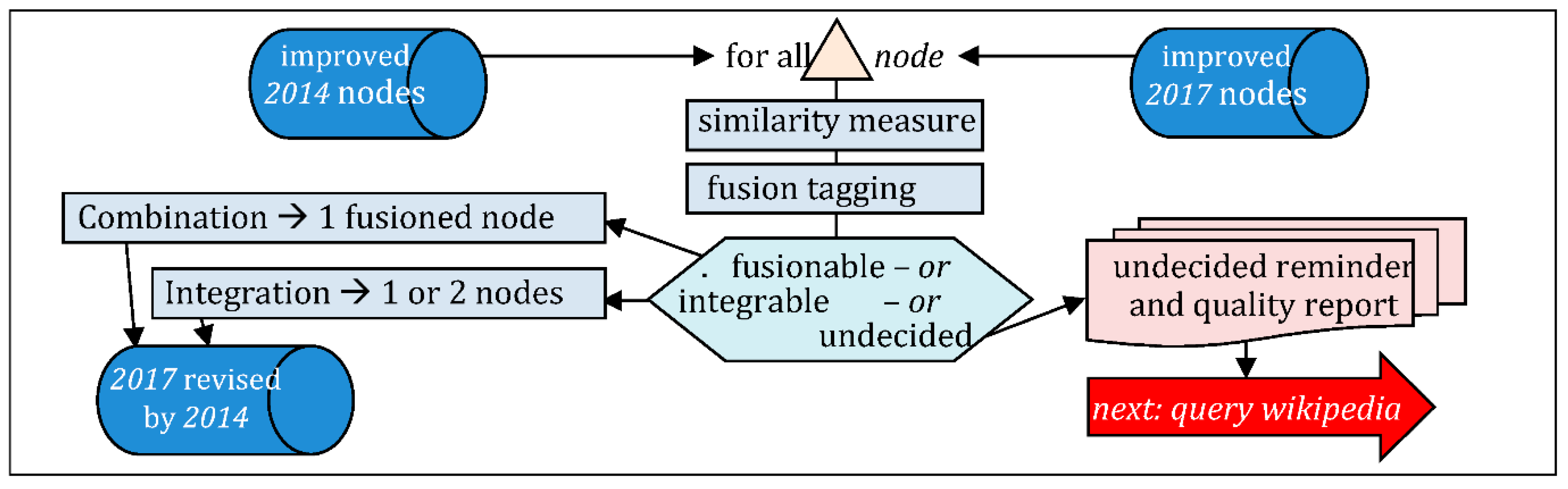
The expectation is that Sncf2014 and Sncf2017, either confirm each other on some nodes, or add up unique nodes (Figure 3).
The relational approach, although natural with tabular-like datasets, has been refuted by the meta- analysis, which revealed that 1525nodes have poor or no geometry, and that label is not a reliable attribute.
Let’s consider instead the fusion approach, following Bloch [12]:
definition.
Fusion of information consists of combining information originating from several sources in order to improve decision making.
More precisely, let usconsider the context of Revision, or reverse-Updating [13] for we aim at reconstructing the past. Revising Sncf2017 by Sncf2014, means to compute in order to undertake “pairing” (2014) with a (2017), then merging attributes with those of , or “impairing” , if no fits, then adding into Sncf2017, after some conversion. All “impaired” of Sncf2017 remain unchanged.
Following Bloch, three steps are required: measure, decision, combination.
2.4.1. Knowledge Representation and Measure of Similarity
Consider a declarative approach based on the notion of neighborhood V(x) of a node x, and a measure of membership to that neighborhood:|y∈V(x)|, degree of similarity of another node y to x.
The meta-analysis tells us that, once duplicates and ambiguities are solved, a dataset is complying with the target constraints, and has an attribute space into which to define “neighborhoods”, and to build a “similarity” measure (Table 7), which is a function , where 0 can be interpreted as false and 1 as true.
Let usdescribe that similarity/dissimilarity measure components:
- (a)
- and () quantify num, label, geometry for both x and y, into the [0, 1] interval;
- (b)
- is qualitative (true/false: 1/0). Checking equality on slug(label) rather than on label;
- (c)
- uses threshold values D1and D2, () uses D3 and D4, whichmeans that dissimilarity is not the complement of the similarity measure.
The initial step is to seek, for each 2017 nodey, the closest 2014 nodex:
to form a pair of “closest nodes”, using the GreatCircle algorithm, whose precision is sufficient in this application, in the range [0, 100 km]. This routine is part of Annex A.
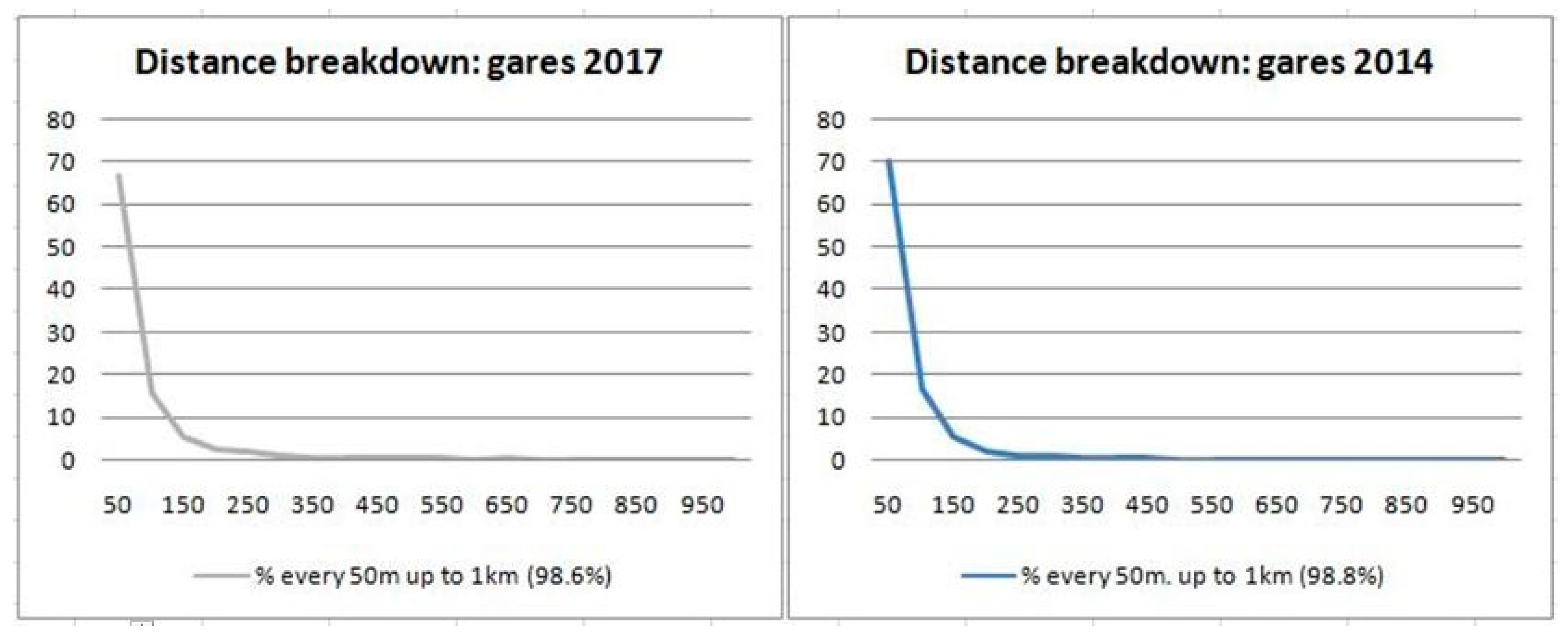
Table 8 gives the distance breakdown for “direct pairs” = pairs of closest nodes with the same label, and “reverse pairs”, with the closest 2017 counterpart of each 2014 node.
The histogram of the distances grouped by 50 m intervals (Figure 4), provides a clue about choosing relevant thresholds:
- the number of directpairs (left) decreases rapidly up to 150 m (88%), and slows down after 300 m (93%); and for reversepairs (right): 92% at 150 m, 96% at 300 m;
- both kinds of pair are less than 1.5% after 1 km; and only a few after 2 km.
Therefore the choice for D1–D2 is 150–300 m, and 1–2 km or D3–D4.
2.4.2. Decision to Include a Node in the Similarity Neighborhood
To include x in class Ci according to the absolute majority (or threshold rule):
- α means: at least % of the nodes of V(x) must be in Ci
The inferential aspect of the declarative approach [14] ensures that:
- (a)
- rules are independent of the actual knowledge in the knowledge base;
- (b)
- rules are not restricted to the conceptual schema representation.
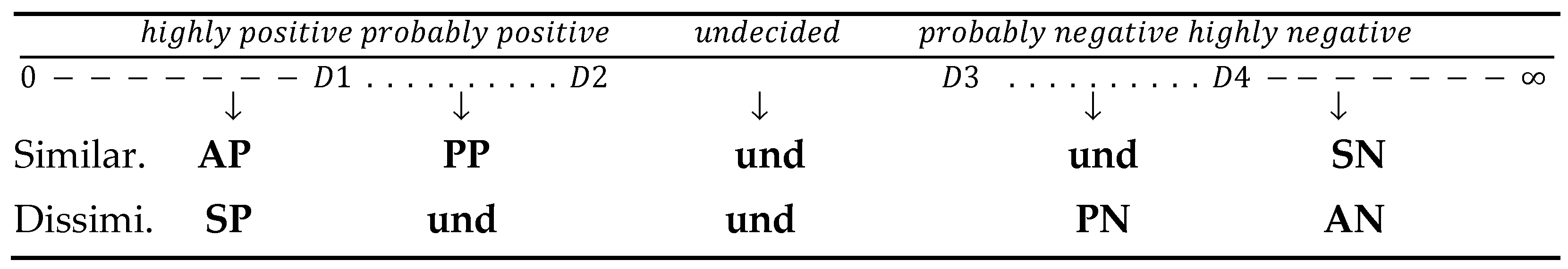
The choice to “pair” x and y is made by comparing |y∈V(x)| to some threshold, causing to keep x and y whose distance is α between D1 and D2: x and y are “positive” candidates to fusion. The uncertainty is that some of them can be “false positives”. Similar nodes, whose dist≥ D4, are tagged “supposed negative” (SN).
The choice to “impair” an x, is to consider, using D3 and D4, that xcannotbe compared to any y, and is candidate to be “integrated” to the final result. However, we may get “false negatives”. Dissimilar x whose dist ≤ D1, are tagged “supposed positive” (SP).
About “undecided” (und) nodes, the choice is between: (1) to reduce the D2–D3 gap, even to D3 = D2, whichreduces the number of und, but increases the number of both false negatives and false positives; or (2) to obtain only a few FNs and FPs, and many undecided.
The overall tagging decision is sketched in Figure 5, with different possible tags.
Corresponding results for direct and reverse revision, are provided in Table 9 (a,b), where signs + and ¬ denote respective use of similarity or dissimilarity measure. Undecided cases (und) are grey cells. Counts for the direct revision do not include the nodes with no geometry.
The role of the fusionTags routine (Appendix A), is to set the tag value (AP, AN, PP, PN, SP, SN or und), of every node and to store it together with the closest counterpart node and distance of that pair, resulting in:
- 2017-node: f + {“tag”:tag(f), “dist”:dist(f,g′), “closest”:link_to-2014(g′)}
- 2014-node: g + {“tag”:tag(g), “dist”:dist(g,f′), “closest”:link_to-2017(f′)}
dist(a,b) measures the distance between node from A and its closest B counterpart.
Then a fusion sort is made into three classes, fusionable, integrable or undecided:
- fusionable: means that the node and its counterpart (closest is ok) are supposed to inform the same real gare and we can proceed with the fusion of their data;
- integrable: means that the node has no counterpart (closest is irrelevant) and can be kept as is (if in the right set), or adapted for integration (if from the other set).
Using f for 2017 and g for 2014, the decision follows the rules:
- -
- direct revision:
- -
- reverse revision (for integration of “forgotten nodes”):
Among the tags, only AP, PP, AN, and PN are reliable enough to be used in the decision. Indeed, we must question the SP-pairs (dist < D1, ≠label), for most uncertainty is due to the toponym-pattern (Appendix B.1). Also we must question SN-pairs (dist > D4, =label): see fork-pattern (Appendix B.2).
Theses tags and distances are helpful when confronting extra open data, for instance with a specific lexicon, e.g.,: Insee-new list of toponym changes, SNCF list of gares at different dates (see Section 3). Also helpful for further processing is the quality of the fusion decision which can be a fuzzy measure between [D1, D2] or [D3, D4] respectively:

2.4.3. Fusion Combination, Integration, Revision and Conclusion
The last fusion step is to make a single “fused” node from a node pair, that is choosing appropriate values for every attribute, e.g., best coordinates?, or to convert into the attribute schema of the other dataset.
The fusion-combination of 2014 attributes concerns:
- -
- nature: which can be translated into a capa value (though losing some specificity).
- -
- geometry: the maximal distance being D2, use 2017 coordinates;
- -
- info: add approximation info about geometry (depending on dist).
The integration of 2017 nodesis straightforward.
The integration of 2014 nodesis more difficult, concerning:
- -
- geometry: straightforward, use 2014 coordinates;
- -
- nature: translate into a capa value (rather easy);
- -
- km: seek for the closest 2 nodeson the same ligne, then interpolate a value;
- -
- uic: build a unique code using numand km;
- -
- info: add uncertainty info about km and uic.
The revised dataset is the new “baseline-resource” for the rest of this work. It complies with target constraints (see metadata: Table 10). Quality information is added whenever an approximation is made.
Overall conclusion before Section 3:
- -
- Software fusion is safe (6415 AP + PP tags = almost no false positives);
- -
- Software integration is safe (74 AN + PN tags = almost no false negatives).
- -
- The remaining 250 nodesfrom 2014 and 564 from 2017 for which the fusion decision is too uncertain, plus 718 with no geometry, from 2017are in total 1532.
The important information after the fusion is that:
- -
- 6489 nodes have been qualified;
- -
- 1532 nodes (label-num-km) -i.e.,: about 950 gares− can be confronted to VGI and remote sensing imagery for setting a controlled geometry.
3. Materials and Methods Part 2: Voluntary Geographic Information (VGI) Data Integration and Control
So far, the revision process has yield an important and consistent dataset, complying with target constraints (unique code, revised label, correct km, …), plus some quality information. However, the target horizon, amounts to twice as manynodes.
Doubling up the total, starting by investigating the 1532 nodesleft behind, then discovering thousands more “forgotten” gares, and further improving the overall quality are the challenges that we ask the VGI to help us overcome.
This section investigates Wikipedia, focusing on its semantic aspect, which makes profit of the UIC ontology (Section 3.1), then investigates various VGI sources, developing some helpers to integratesparse data from less structured and less semantic web data, and it takes advantage of the aerial pictures archives made publicly available by the French IGN.
3.1. Gathering Information from Wikipedia Railway Specific Pages
There are many pages devoted to railways. Luckily, standardization efforts of the UIC (UIC: Union Internationale des Chemins de fer, the Worldwide Railway Organization, since 1922) propose an international ontology (thousands terms in the UIC railway Dictionary), allowing the design of semantic Wikipedia “templates” for gares, lignes and communes.
3.1.1. Extracting Coordinates from Wikipedia
Let usstart with a simple use: the extraction of the coordinates of a gare named label.
The Wikipedia API (application program interface) gives access to the coordinates, at the highest level. Querying it with “Gare de label”, returns the coordinates (if any), or “missing”.
The wikiCoordinates routine (Annex) is an asynchronous code that must be used in a “Promise” (technology to awaiting answer, provided by most computing languages).
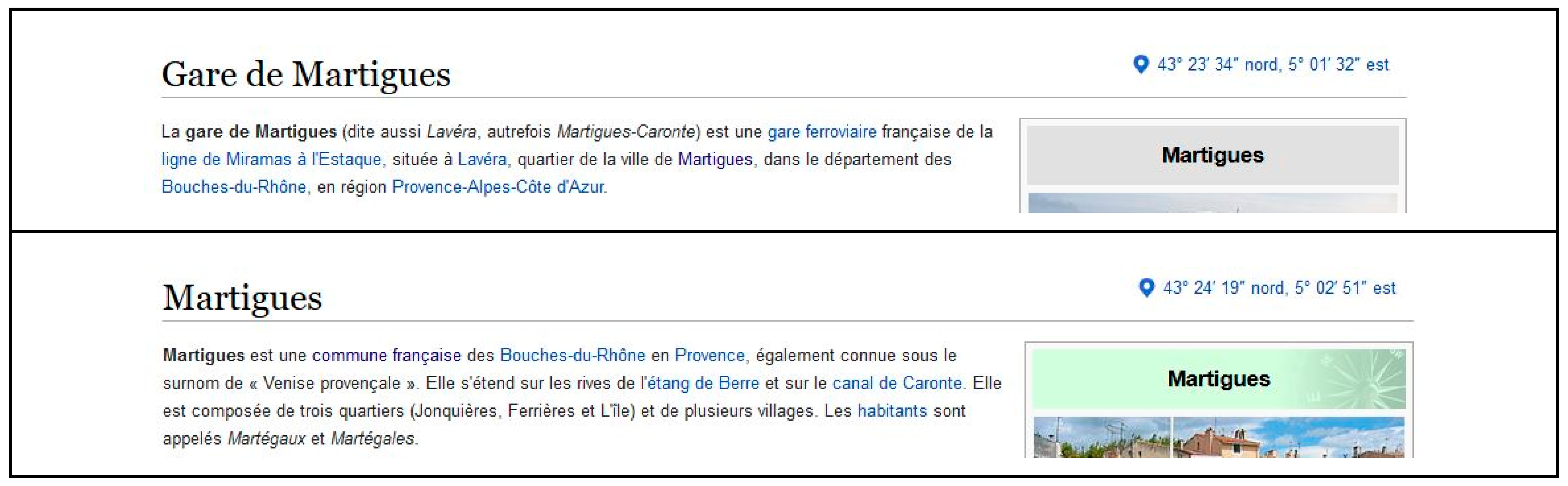
In case of a “missing”result, we can query the API with “label” as commune toponym, for quite often a gare is labeled by its commune name. However the gare can be somewhat far from the center. For instance, with Martigues (Figure 6), the distance is 5.3 km (great-circle distance). Therefore, coordinates obtained by that means provides only a rough positioning, which may help when using remote-sensing imagery.
The wikiCoordinates routine is used for improving the “revised” dataset, when several location compete for one label, for instance, in the case of Saintes (Section 2.3), the distance between the duplicates was 348 m, and the answer of wikiCoordinates is:
Query:”Gare de Saintes” → geometry:[−0.617596,45.748672], Quality:”good”
That result is removing the uncertainty.
3.1.2. Extracting Semantic Information Using Wikipedia’s Infobox
The Wikipedia API-v2 provides much richer information from an “ontology-driven” Infobox [22].
An Infobox is a panel, usually next to the lead section, which uses a specific ontology:
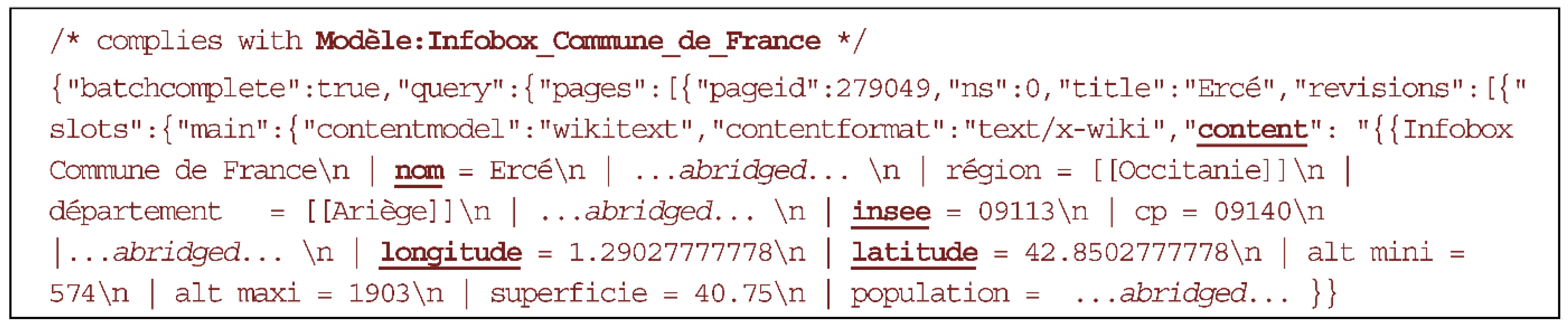
- commune:{{Infobox Commune de France}} contains coordinates, insee and more (Figure 7);
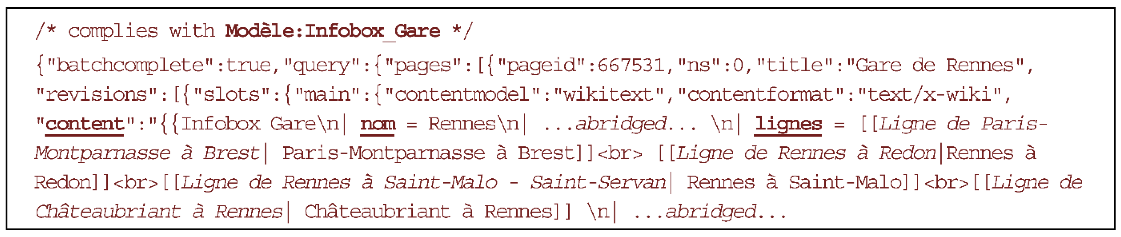
- gare: {{Infobox Gare …}}, contains coordinates, nom of the including commune, all or some of the lignes that connect to that gare (Figure 8).
- ligne:{{Infobox Ligne ferroviaire …}} see next Section 3.1.3.
The routine wikiInfobox (Appendix A) can parse both types of Infobox.
3.1.3. Extracting Data for all the Garesof a Same Ligne: The Routemap Semantics
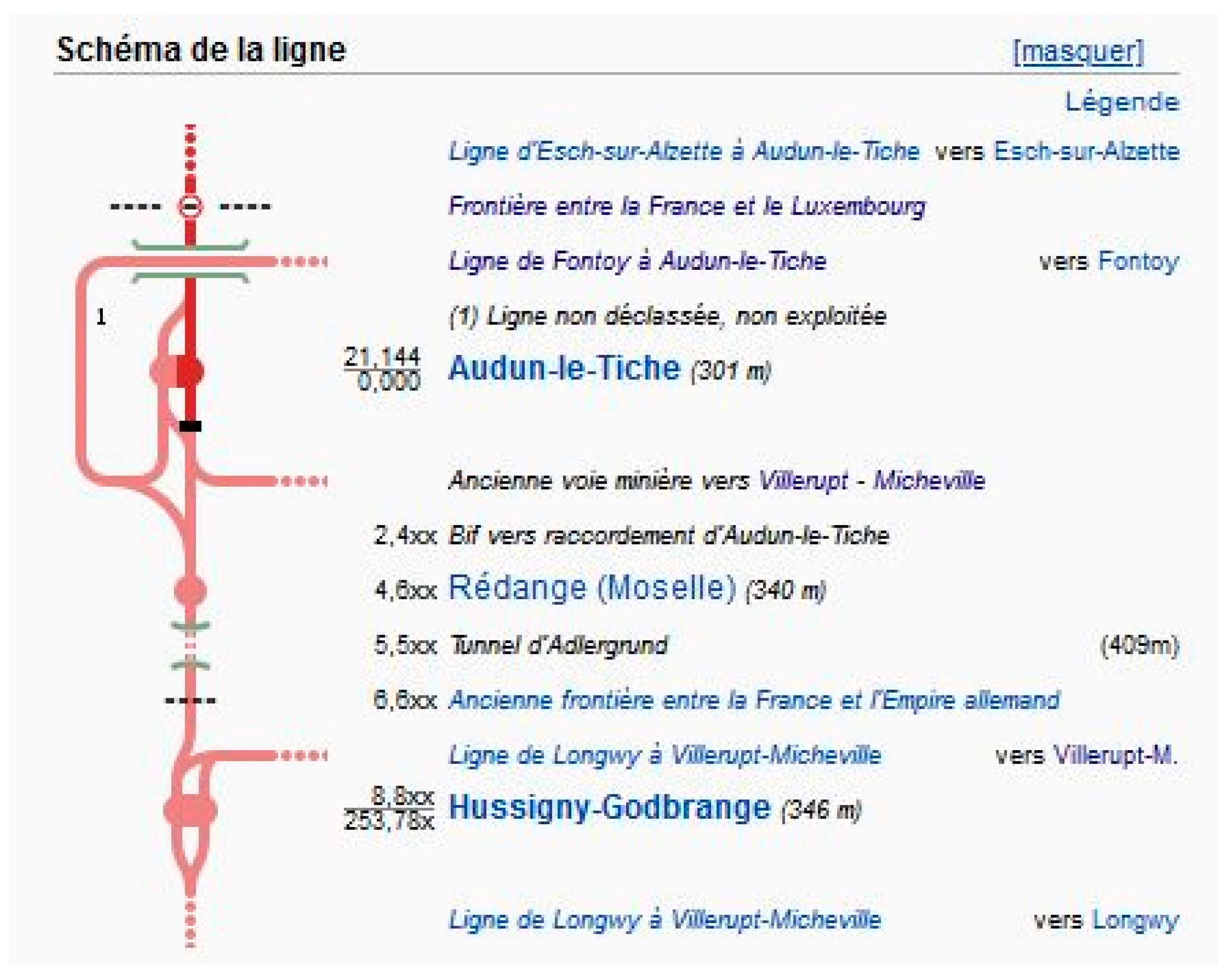
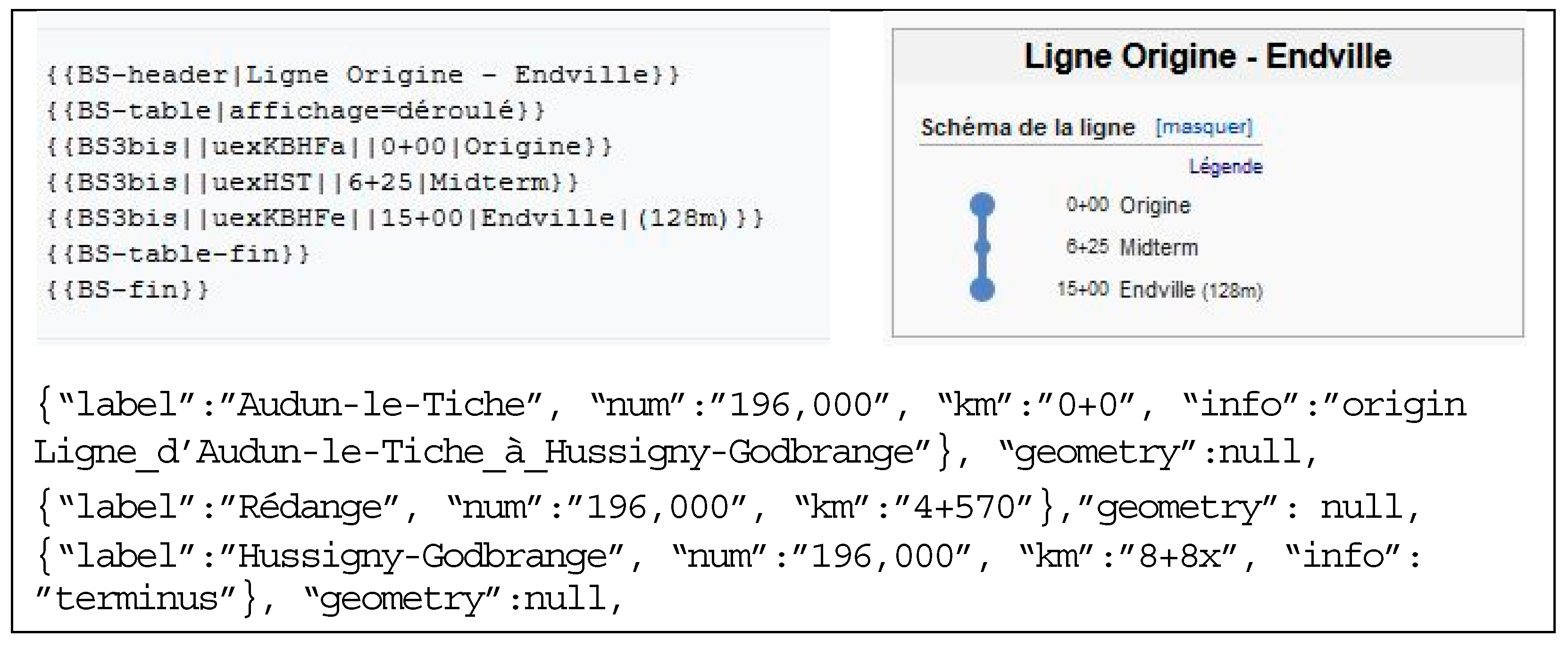
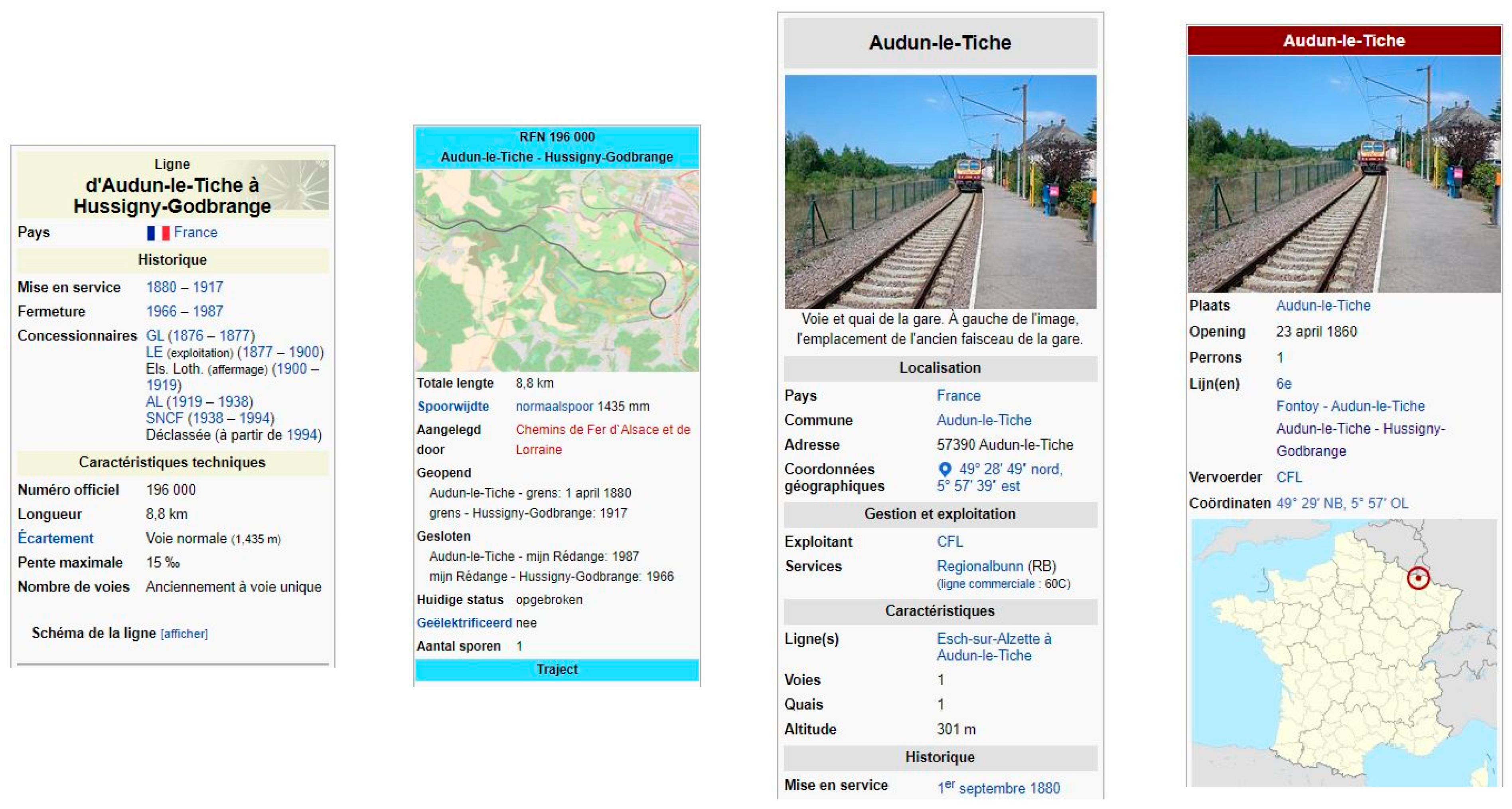
Given a ligne name, e.g., Ligne_d’Audun-le-Tiche_à_Hussigny-Godbrange, we can query the Wikipedia API, and get an {{Infobox Ligne ferroviaire …}} description.
That Infobox (French template) contains simple items, such as length (longueur), gauge (écartement), the official num (numéro), closing date (fermeture), …, and a much more complex item: a table whose syntax is intended to display a “routemap” (schéma) of that ligne.
The routemap semantics (French sites,) refers to Modèles/BS (“BS” stands for BahnStrecke for the model has been initiated by Germans). English sites refer to the general Route diagram template description [33,34].
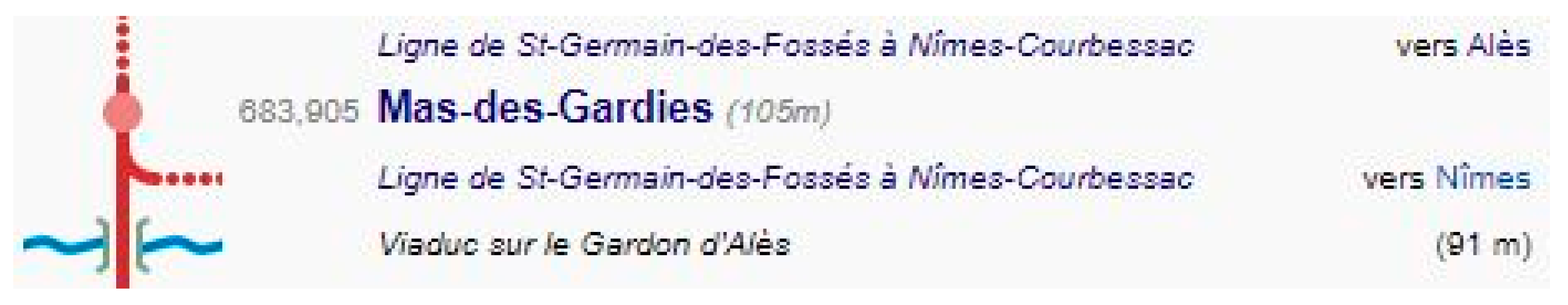
A simplified version of a ligne Infobox, is in Table 11. The “schéma” extracted from this Infobox, is presented in a simplified version, in Table 12: it is a {{BS-table}}, complying with the BS model, which gives the ordered list of nodes, along that ligne.
The right column indicates which attribute to be parsed (values underlined on left): origin to terminus, gares with label, km, also forks to other lines, bridges, international border crossings, etc.and most of the expected information, except the geometry.
Wikipedia parses the BS-table to draw a graphic representation of the ligne (Figure 9).
There are 1000 such Wikipedia pages for French lignes, each ligne being linked to one or several other lignes. Therefore, it is worth developing a specific routine for the parsing of an Infobox and its BS-table.
However, the hard part is twofold:
- the Infobox BS-table complies with Modèles/BS, whose syntax is somewhat tricky, but was parsed successfully in most cases: only a few code failures, hard to overcome, have been met. Figure 10 illustrates a simple case of {{BS-table}}, code and result.
- The other difficulty is to deal with the cascade of asynchronous Internet requests for processing a single line.
Attributes are set from the parsing:
- num is in the Infobox main part (Infobox attribute numéro = 196,000);
- label, kmare in the BS-table, and km can be interpolated, if absent;
- nom is often given (if differing from label), insee must be determined later;
- geometry is null, but can be seekon ‘Gare d’Audun-le-Tiche’, ‘Gare de Rédange’, etc.
Routine wikiBSTable (Appendix A) shows how the parsing of one table can trigger a cascade of asynchronous requests: initial fetch, possible second fetch if there is an indirection on the BS-table, then a fetch trying to get the geometry of each individual gare found in the BS-table. The full code is much longer, and out of the scope of that paper.
Moreover, when parsing a ligne, one or several connected lignes can be found, and for every such ligne, we can trigger a new request for that new ligne, and so on. Piling up these requests should in theory allow us to browse the entire network, but in practice rapidly saturates memory and computing resources, at least on a personal computer.
To develop a full scale “big-data” procedure would improve greatly the time spent linking data, from lignes to gares, and from gares to their geocoded location. Instead, we are querying Wikipedia with only a few (2 to 4) lignes requests at a time.
3.2. Gathering Information from VGI Pages
Wikipedia is a great, irreplaceable source of collaborative VGI, covering almost the full range of the lignes that have been included in the main French railway network. However, “secondary” lignes (rural lines and tramways), which were never embraced in the nationalization of 1937 into what became the SNCF [27], have not yet been treated so extensively: a dozen or two are fully described (with BS-table). About 100 are qualitatively described in the page of their owning operator, e.g., “Voies_ferrées_des_Landes” lists 12lignes, only two having their specific page (w/o BS-table).
However, in France as in most countries, railways arouse vocations for “volunteers”, and a lot of French websites (Table 13) are devoted to keep track of past gares, lignes, viaducts and tunnels. Even the collection of street-signs (“place de la gare”, “rue du petit-train”) is valuable: it is the toponymy-memory of the location of a past gare.
The variety of information, and unstructured representation, make it difficult to code any generic software. But some routines may help, which are proposed in thissection.
There are two critical steps in the overall process described in Section 2.1.3:
- -
- First step(a): identifying the existence of a gare onto a ligne;
- -
- Last step(d): obtaining coordinates data.
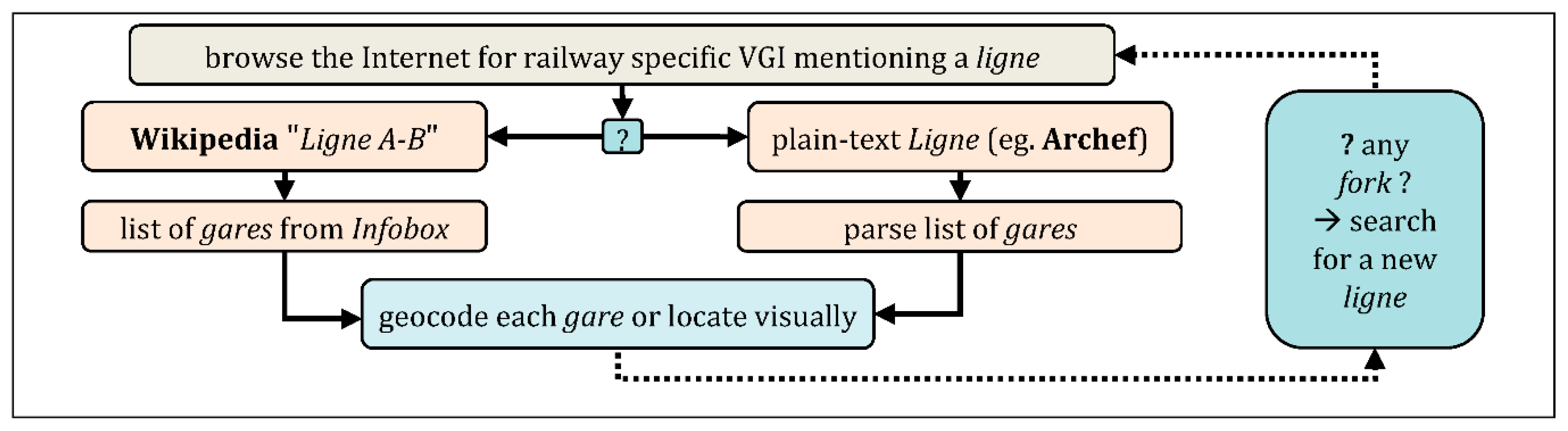
The generic approach to extracting gare information from VGI starts with step(a): fortunately, most mentioned VGI providesome data, loosely structured by ligne (be a text or a table), for instance:
- “ligne A to B has such characteristics, and comprises: gare1, gare2 ... ”,
- The challenge is then to code a “parser” that delivers a list of nodes such as:
- {label:“A”, num:“AtoBcode”, km:“0”, info:“origin of A to B, characteristics“}
- {label:“gare1_name”, num:“AtoBcode”, km:“somerank information, or 1”}
- {label:“gare2_name”, num:“AtoBcode”, km:“somerank information, or 2”}
- …
- {label:“B”, num:“AtoBcode”, km:“max = length, or max rank”, info: “terminus”}
Here, follow three cases that are common among several VGI.
3.2.1. HTML-Style Tables
As opposed to a Wikipedia Infobox, the HTML <table> tag is not a semantic tag, and it is uneasy to determine its content, unless by direct reading (no simple artificial intelligence (AI) routine at hand, although research is becoming active). For decision making, the most important question is:
- is there a relevant key in that table? (e.g., num, insee, label?).
A few cases, from Routes or RDrail, were processed this way, giving information only about origin-terminus, and some ligne characteristics (closing date, gauge, length):
- visual: make a decision about relevance;
- manual: copy and paste the table text into a spreadsheet; convert into CSV format;
- software: fetch CSV file; join objects with routine mergeLigneInfo (Appendix A).
3.2.2. Coordinates Lists (Polyline for a Ligne) in Google KML or GPX Format
Some contributors have digitalized lignes using the GoogleMyMaps facility, and sometimes, gare are individualized in such kinds of data. The procedure is:
- manual: export the ligne data into KML format (from the Google page);
- software: convert into geojson, and if the gare is individualized: add it directly, or:
- manual: copy and paste the relevant geojson of the ligne;
This has been used with source Traver and a few lignes from cdfFR (Table 13).
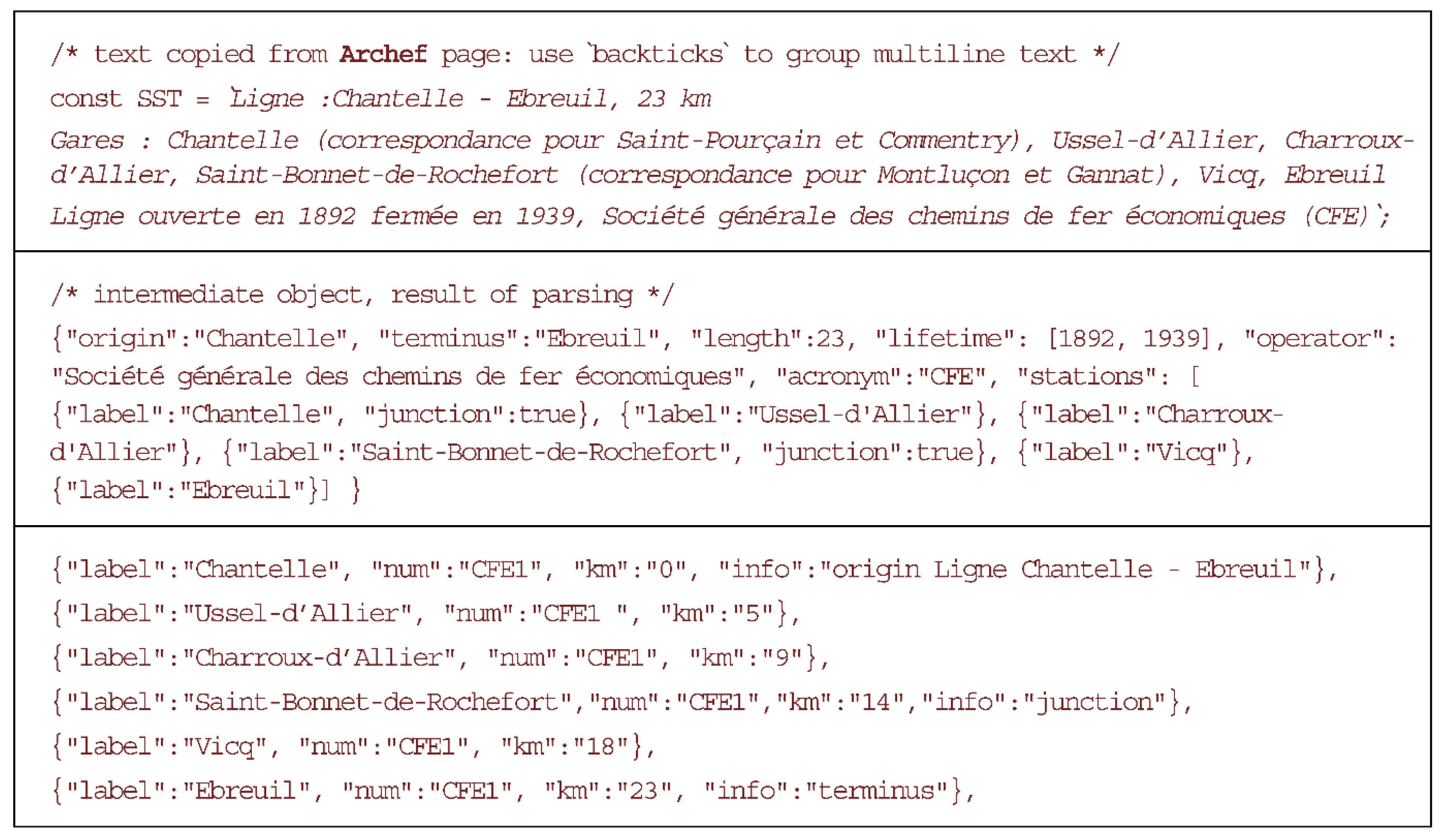
3.2.3. Simple Lists of gares in Plain Text
It is not easy to automate a detection, but the result proves useful in obtaining a list of gares along a same ligne:
- manual: copy-paste the text into a string constant;
- software: check if that ligne is already documented, or add a new ligne number num.
The routine stationsAlongLine (Annex) is used in parsing the example of (Figure 11).
Parsing the text extracted from one page of Archef provides an ordered list of gares, from origin to terminus, a length, creates the lignenum, and two dates for its lifetime.
3.3. Remote-Sensing Information for the Assisted Visual Geocoding of Gares
If the direct geocoding of a gare (wikiCoordinates) has failed, the last opportunity is to visually inspect maps or aerial pictures to locate that gare, in a way similar to [35] with land-cover.
For geocoding a gare, there is a two-step procedure:
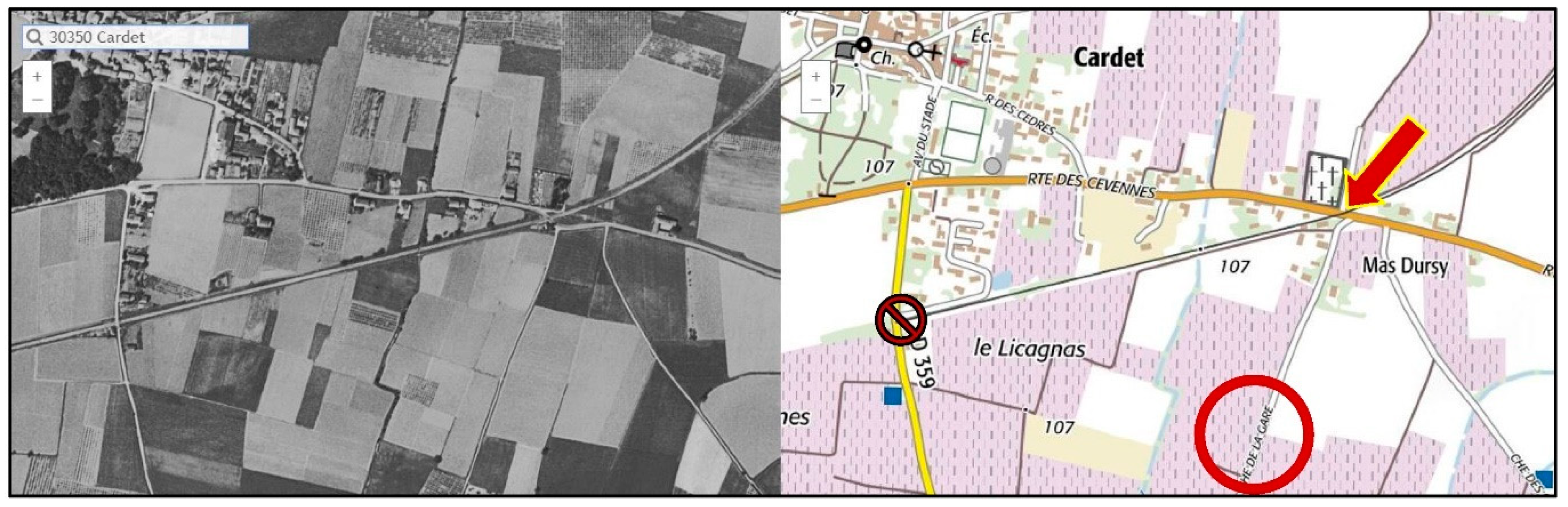
- (1) software: use a geocoder API (e.g., Google), querying coordinates for: French word “gare” + label. For instance, with Cardet (Gard), we can try a few query variants (Table 14). It is impossible to know which query will give the best answer (distance data have been added in Table 14, only after visual inspection);
- (2) manual/visual: use any approximation, or skip first step, and input the toponym into an online map facility providing, preferably ancient, maps and aerial photos.
In France, the best data source for historic (mid-20th century) aerial images and maps, is IGN, the French national geographic organization, which provides the website: https://remonterletemps.ign.fr, giving access to:
- Today (2016–2018): Aerial image (≈1 m resolution), Vector cartography (≈1/10,000)
- Past (1947–1960): Aerial image (≈10 m resolution), Digitized map (≈1/25,000)
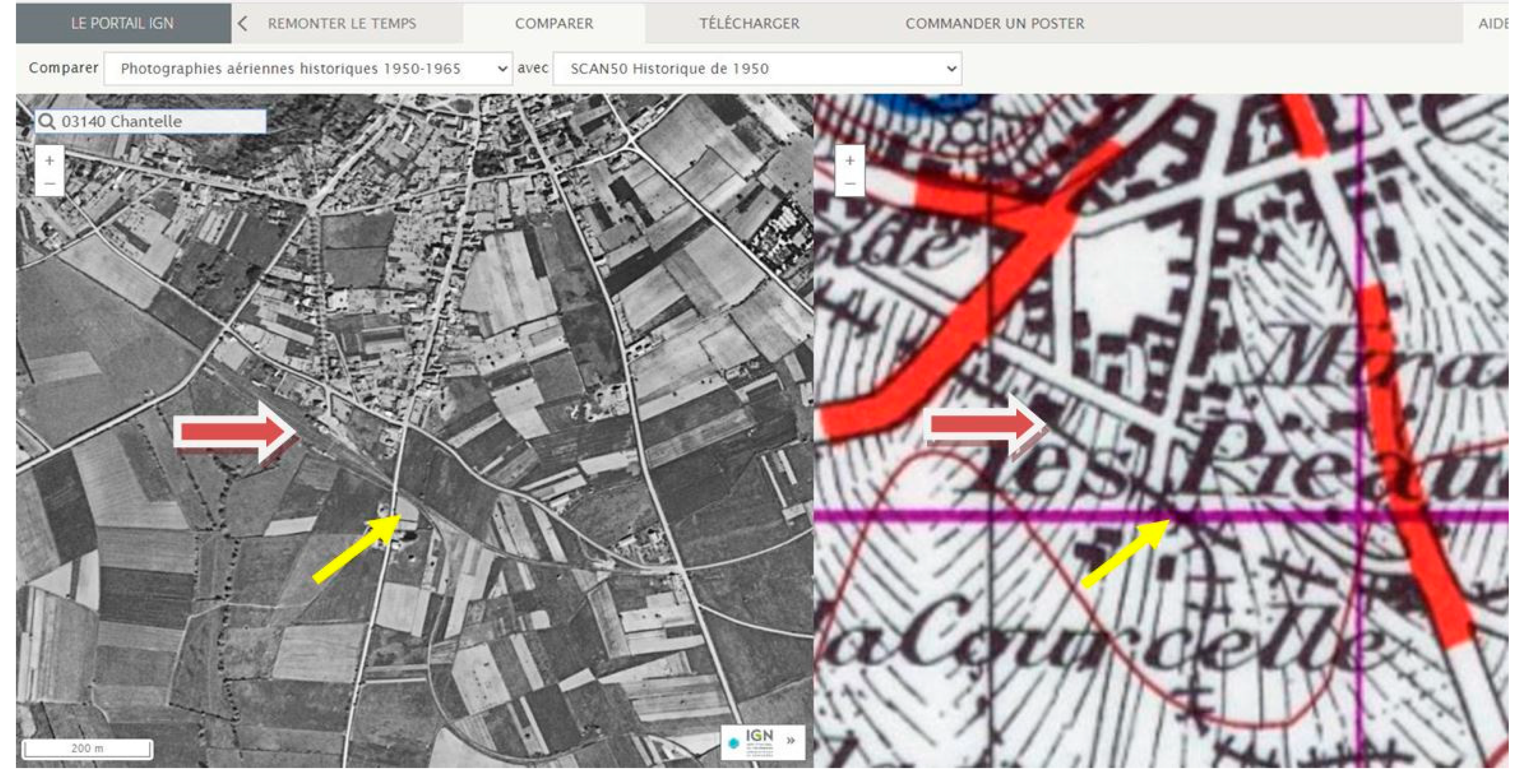
Figure 12 illustrates this website with toponym ‘Chantelle’ (cf. Section 3.2.3), at zoom = 16, and two sources (1954-aerial and 1952-map): the gare is visible (big arrow) and the fork between lines (yellow arrow), about 200 m SW of the gare (scale at bottom-left corner).
3.3.1. Dual Use of the Website RemonterLeTemps, (a) Direct Geocoding of Toponyms
Routine checkToponymAt (Appendix A) encodes the identifier URI pointing to the relevant remonterLeTemps data for a given nom, what we did above with Chantelle (Figure 12).
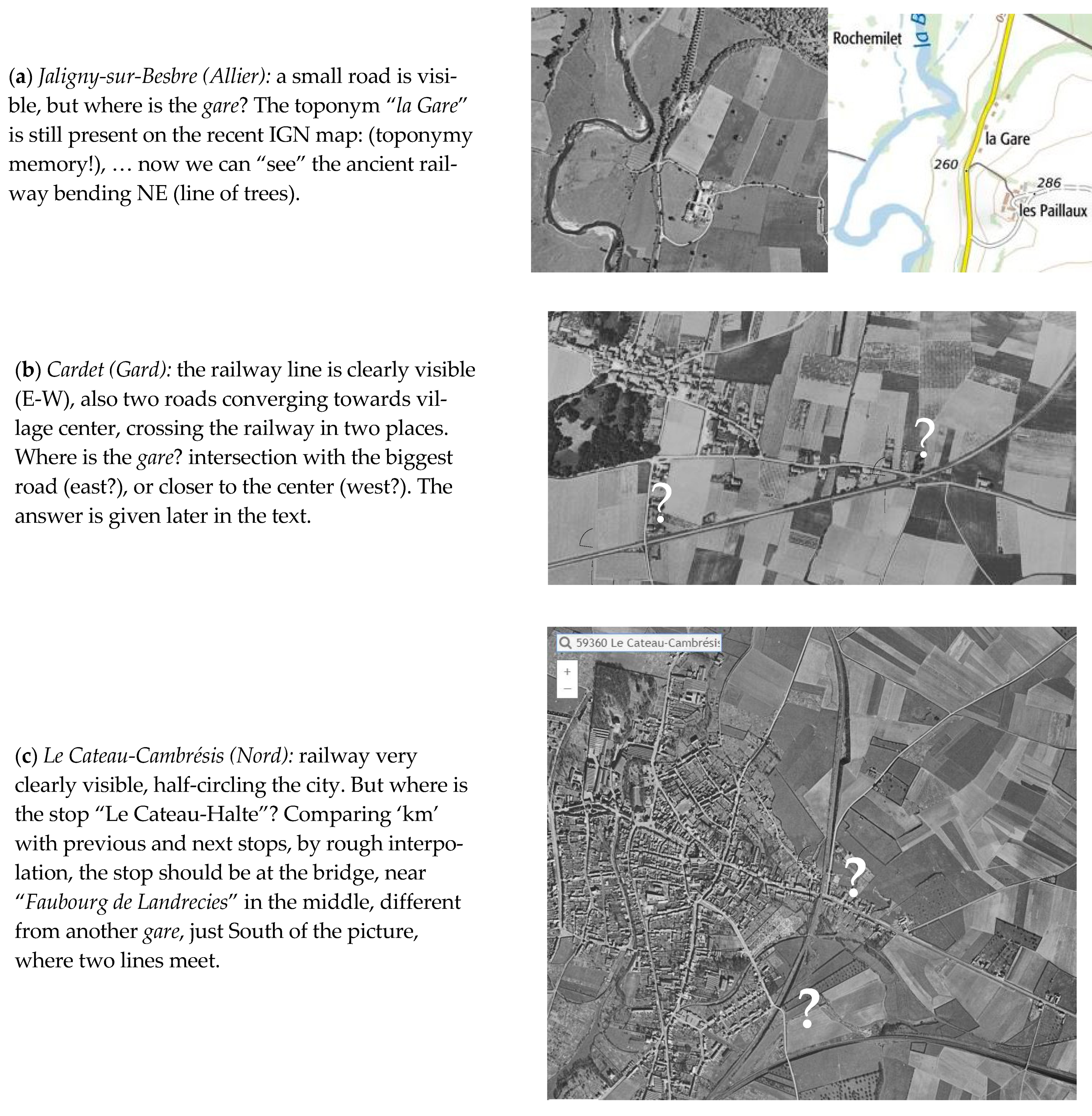
The next step to detecting a gare, is visual: quite often rather easy, sometimes more difficult (cf. examples in Figure 13a–c). A gare is always at the junction of several linear elements (rail + road), easier to detect when finding the appropriate zoom level.
Therefore, the different steps of the procedure can be summarized as:
- software: generate URI using routine checkToponymAt;
- visual: start with an intermediate zoom (e.g., z = 16) and focus on the section where the line is expected to reach the commune (e.g., SW corner);
- visual: inspect map-aerial photo combinations, focus on road-rail intersections;
- manual: input back coordinates into geometry of the gare.
Adding more automation is beyond the scope of this study. The care brought to this task, must insure a high quality, for it will be very difficult to detect errors later.
3.3.2. Dual Use of the Website RemonterLeTemps: (b) Visual Reverse-Geocoding
To show where a geometry points to in aerial or map representation at a given date:
- software: generate URI using routine checkGeocodeAt (Annex), cross-check with a geocoder, to get commune name;
- visual: start with a high zoom (e.g., 19), and inspect map-aerial photo combinations, zoom-out to get neighbor toponyms (railway terminology may appear);
- manual: confirm, or infirm, the quality of the information for that node.
3.3.3. Hints for Alternatives
Cartography is notan exact science, even at “the scale of a mile to the mile!” (Lewis Carroll), different maps may choose to display different toponyms. Sometimes Bingmaps or Googlemaps may help to solve an indecision, sometimes the “carte IGN”, what is the case for the Cardet indecision (from Figure 13b): the gare is at the East intersection, “Chemin de la Gare” (Figure 14, right), not at the West intersection, although closer to the center of the village.
The problem is to find the right zoom level, which displays the street name.
Note: to the same query: “Chemin de la Gare, Cardet”, the Google geocoder answers a location 563 m (more South), versus 50 m with the IGN geocoder. In that particular case, we have the visual result exactly at the crossing with the road.
4. Results: The Overall Procedure, the Reconstructed Network, and Its Quality Control
There are four main results out of this study:
- the dataset “CARP” of French gares, over the 1920–2020 time span;
- the developed routines combined in a computer-assisted reconstruction procedure;
- quality controls increase confidence, or point out odd/missing data, to be fixed later.
4.1. The Reconstruted Network (CARP)
The Computer-Assisted Reconstruction Procedure –CARP- data result from the fusion (Section 4.2.1) and from the VGI integration (Section 4.2.2). So far, as of January 2021: the CARP dataset contains about 10,900 nodes, accounting for about 9100 different gares (about 100 in neighbor countries), 450 fork nodes, and 68 border-crossing nodes.
Displaying the CARP Dataset
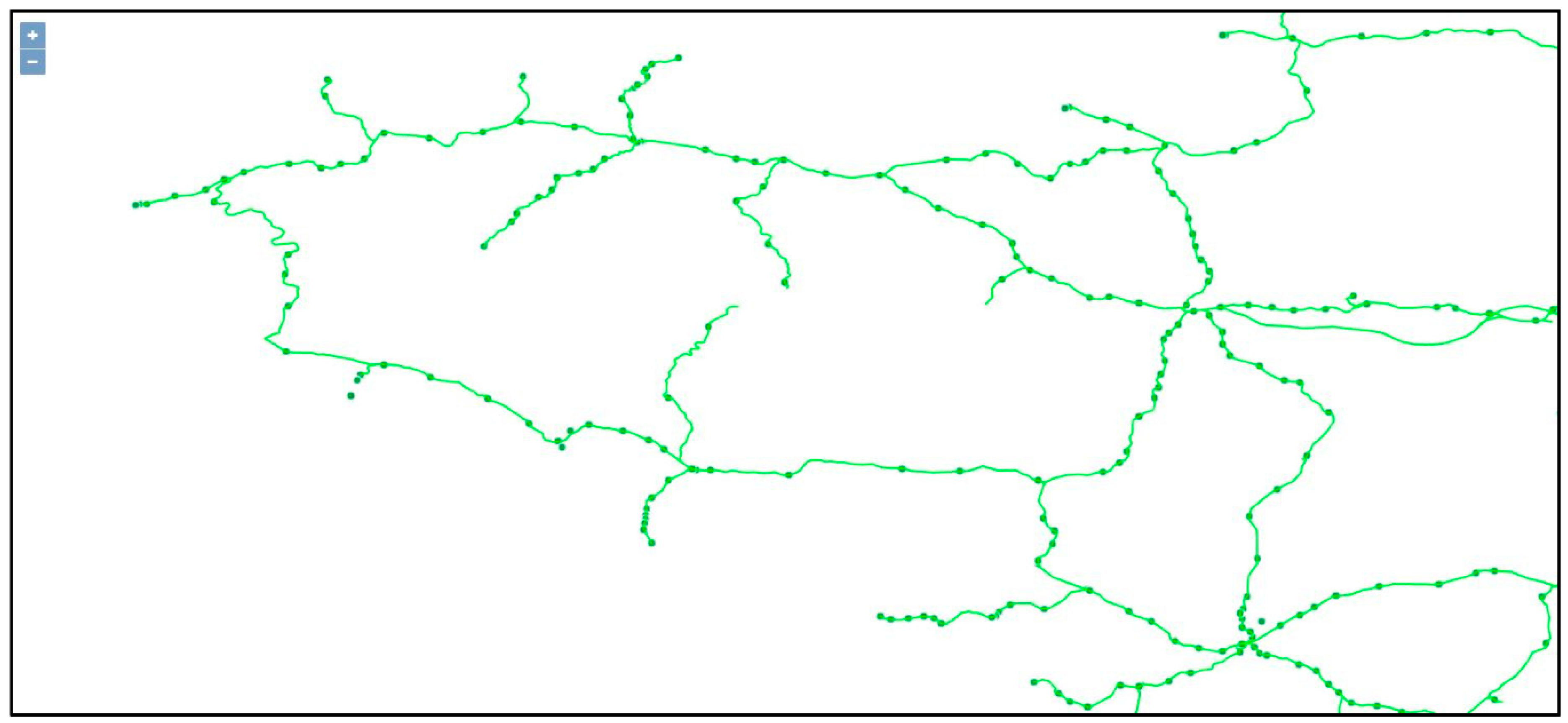
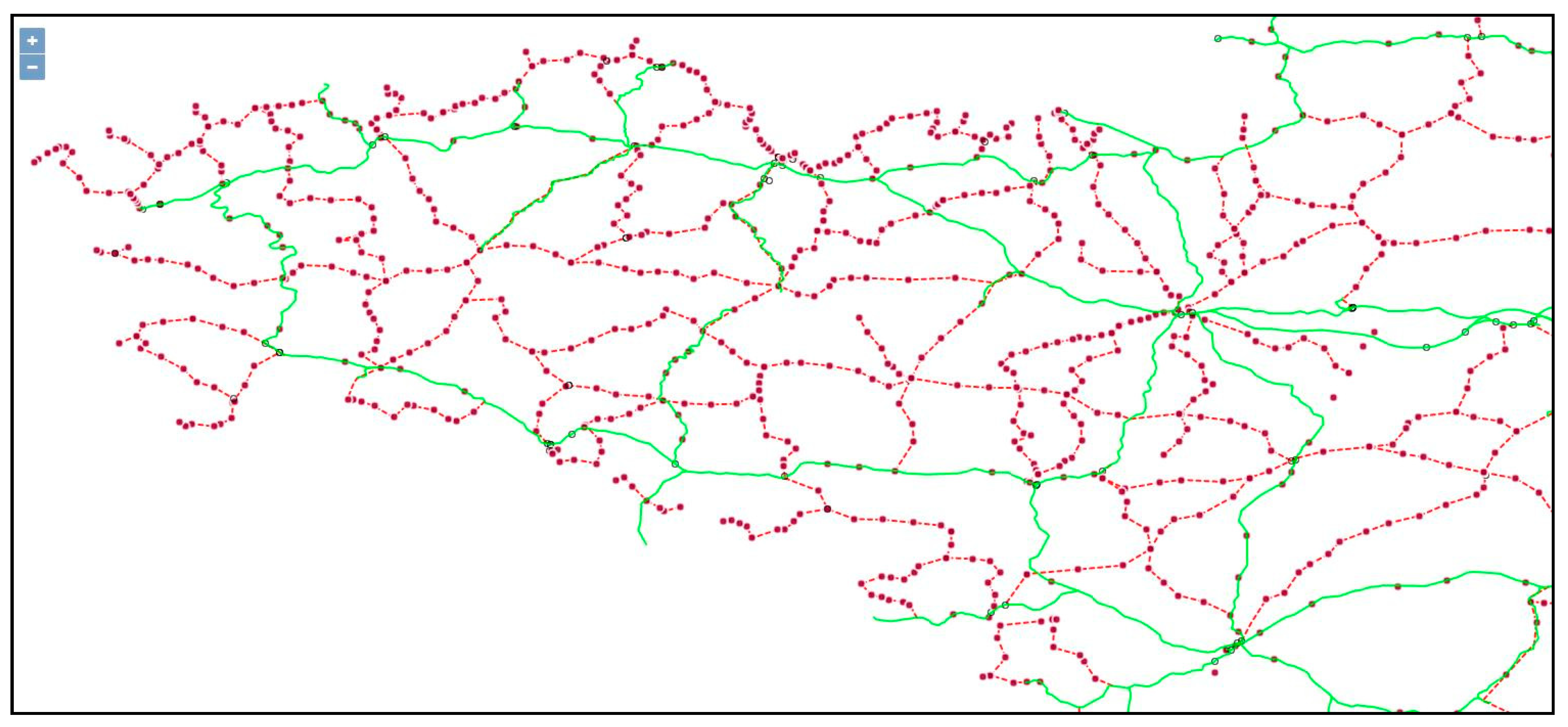
Figure 15 illustrates a part of the CARP on the Region-Bretagne, active gares only are on Figure 16, and disused gares on Figure 17. All data are plotted on top of a classical tiled OpenStreetMap, and green lignes are from the LignesSNCF dataset.
All gares are sorted by ligne, and by km increasing order: it allows a simple routine to convert these sequences into a line-string, plotted as dotted red lines that approximate the disused lignes: no extra information is added.
The Region Bretagne has been thoroughly processed: the CARP data represent almost 100% of what has ever existed. Region Provence is almost complete as well.
The CARP dataset is deposited, under open license, on the data.gouv.fr website. The format is geojson. Periodic revisions will bring additional data until full completion.
The meta-analysis appliedto CARP, has helped in understanding more discrepancies (systematic bias rather than arbitrary errors):
- label disparity due to change between dates: the toponym-pattern (Appendix B.1);
- geometry deviation, due to network evolution and “fork-pattern” (Appendix B.2).
The CARP tries to restore the evolution of the data as best as possible, and to bring additional corrections wherever identified.
4.2. The Computer-Assisted Reconstruction Procedure for Past Railway Stations
4.2.1. The Generic Procedure for Reconstruction from Public Datasets: CARP-Main
Procedures described in Section 2 and Section 3 result in that CARP, summarized in the next two paragraphs:
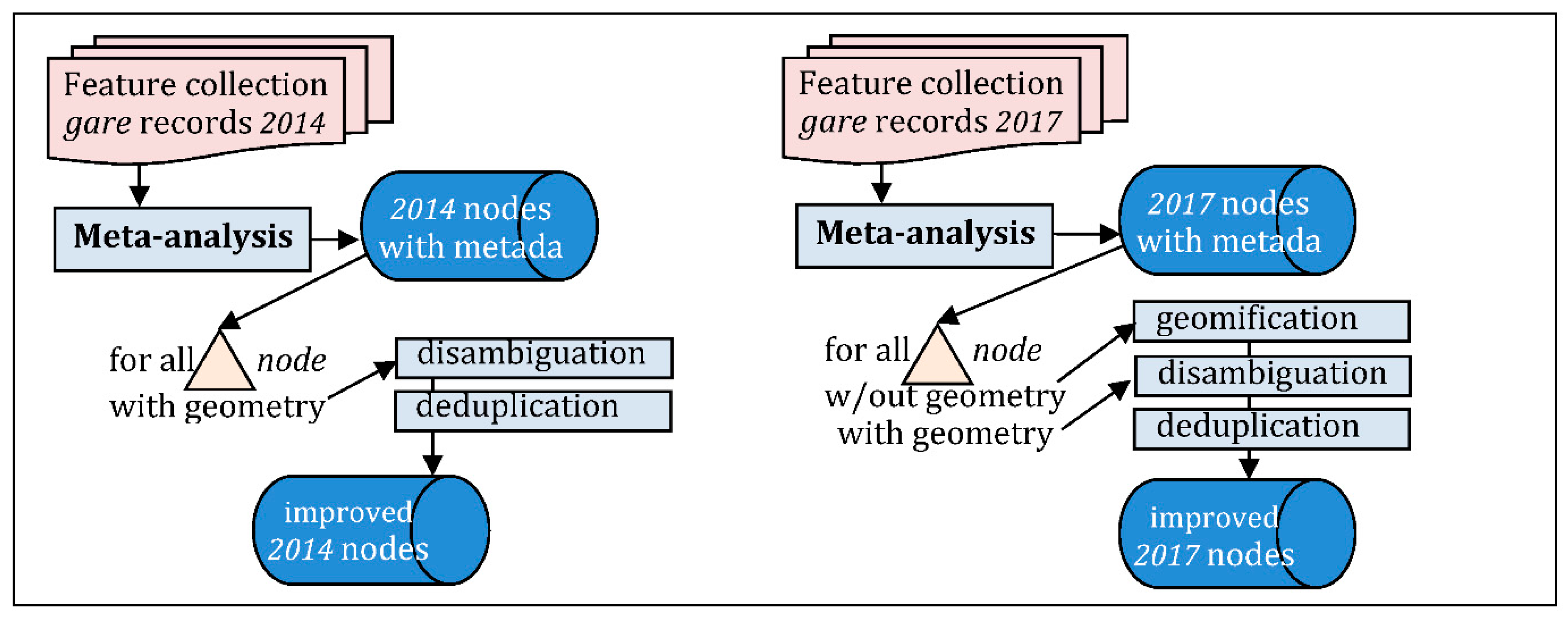
- Meta-analysis (Figure 18): production of metadata, counting missing attributes, checking constraints (e.g., uniqueness), correction of ambiguities and duplicates, possibly completing some geometry, per-node addition of quality information;
- Three-steps fusion: similarity–measure, fusion–decision, attribute–combination (Figure 19), whichyields the revised dataset (=6489 nodes), plus dataset of remaining undecidednodes, i.e.,: no geometry (718), or too uncertain (250 in 2014, 564 in 2017);
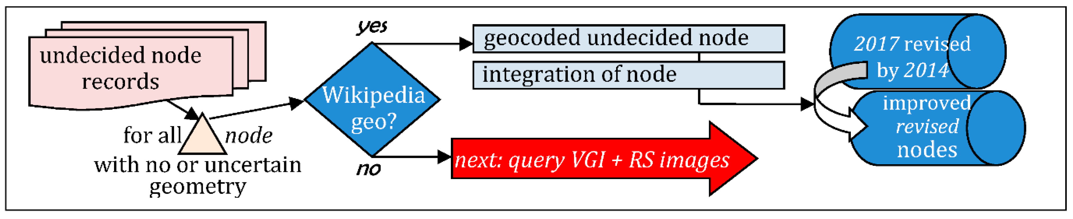
- Quest for geometry of undecided nodes (Figure 20), using Wikipedia or any direct geocoder, to get gare coordinates: it helped to integrate about 400 additional nodes;
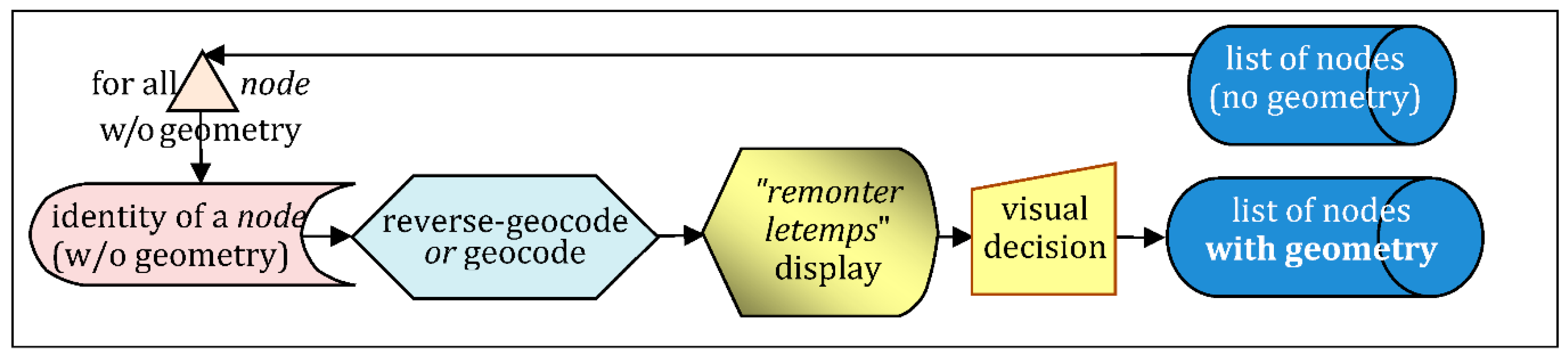
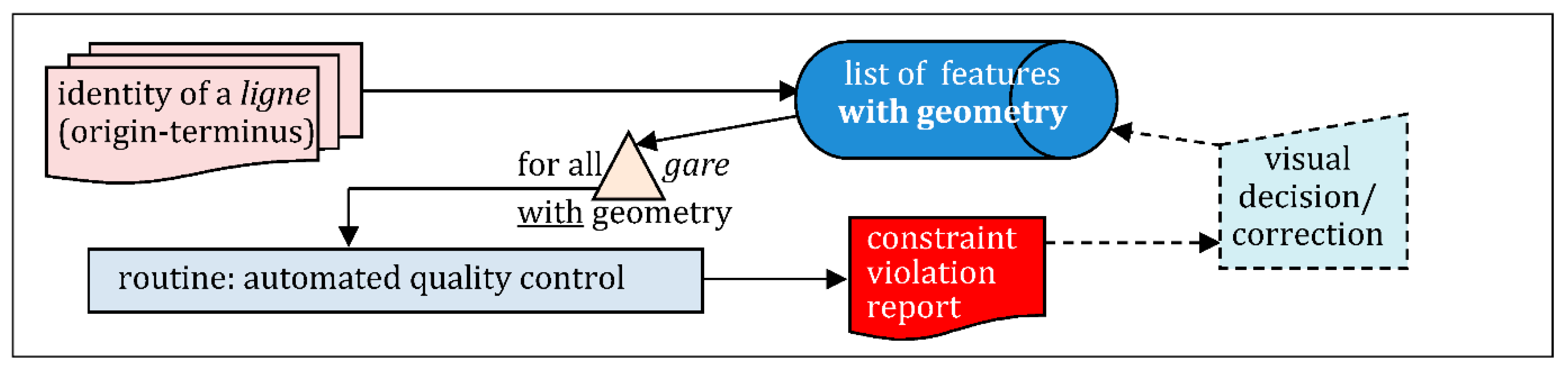
- Visual inspection of Remote Sensing/old maps, for final improvements: it gave about 600 additional nodes originally in public datasets but without geometry (Figure 21).
Only the last step (Figure 21) is “manual/visual”, although assisted by some direct or reverse geocoding, depending on what is available first (toponym, or closest geometry).
The dataset built at this step is named “CARP-main”.
4.2.2. Addition of New Lignesand Gares, from VGI
A gare exists only if a ligne exists to which that gare belongs. Most of the ‘secondary’ lignes are not recorded in public datasets, and have no official num code. VGI has recorded many of them. Depending on what can be found, various routines may apply.
- (a)
- from a ligne: list of nodes (routines executed on the server):f[i] = {“label”:”l”, “num”:”n”, “km”:”k”, “info”:”…”}, “geometry”:null;
- (b)
- f[i].geometry = {“type”:”Point”, “coordinates”:[lon,lat]};
- (c)
- for each node with geometry (Figure 23), check nom and insee, check km strict order, check label uniqueness in CARP dataset, check geometry deviation if a gare of the same label exists already. Report control result in info:{f[i].nom, f[i].insee} = getCommuneFromPoint(f[i].geometry?.coordinates);f[i].info += “ (commune_ok | commune_inconsistent) (km_checked) …”;The dataset built at this step is named “CARP-VGI”.
4.3. Posterior Quality Control, Revealing Additional Errors
4.3.1. Enacting Quality through Constraint Checking
The automated constraint checking is performed a posteriori, checking:
- a gare has a label, a num, and a km, identifying it and the ligne to which it belongs;
- all gares sharing the same num, have their km in strict increasing order, from the gare tagged origin to the gare tagged terminus, what means at least two gares per ligne;
- a gare with an inseecommune code, has its geometry-point inside the geometry-polygon of that commune; every gare located in France can receive an inseecommune code;
- a garelabel is consistent with its communenom and insee. Quite often a label is the name of an existing commune (sometimes 2 communes names).
Rules 1–4 were implemented, It helped to reporting a few dozen inconsistencies, e.g.,: about 60 ambiguities, and a dozen duplicates were identified and corrected. Only a few having required a manual correction, and only one was interpreted as an arbitrary error identified so far. Some cases revealed a ‘fork-pattern’ again, such as this example:
- {“label”:”Lézan”, “nom”:”Lézan”, …“coordinates”:[4.11488, 44.04241]},
Checking coordinates, rule 4 answers: nom = Vézénobres, about 7 km East of Lézan.
The Wikipedia Infobox:schéma (Figure 24) indicates the fork just before the viaduct.
Result: fork-pattern again, discovered by the final computer-assisted quality control.
4.3.2. A Posteriori Control of the Reconstructed Network
The result for CARP is everywhere better than Sncf2017, and in particular the lignes are much better represented with CARP.
5. Discussion
This paper has focused on designing a computer-assisted reconstruction procedure with the goal to gather as many gares as possible from any kind of available source of information. Several software solutions were considered and then abandoned forrequiring too much development (concurrent cascading queries), or for having too little expected benefit (deep machine-learning gare detection, based on already learned gare locations).
Because the spectrum is rather large, we need some guidelines to assess the overall method from an organizational point of view (Section 5.1). Then, to open some perspectives in possible applications, one example is given in Section 5.2, and in European cooperation, because it was the initial motivation of starting this work: to understand how a century of French transportation policies has led to shrinkage of the national coverage so much, what shifts cargo transportation to roads, and what scientific arguments to reverse that policy trends are important. This can be grounded on historical analysis, in comparison with other European countries that have, or have not, followed the same trend in rail transportation policies (the author’s feeling is that important differences can be revealed).
5.1. Theoretical Issues in Building a Comprehensive Dataset from Internet Sources
The problem of building a dataset from the vast amount of information available on the Internet has been theorized, noticeably in the medical sector, for instance by Sreenivasaiah et al. [36], which lists four categories of a total 11 issues for integrating information. This present work is confronted with at these categories.
5.1.1. Data Representation and Standards; Interoperability; Data Visualization; Issues in the Development of Tools
These four issues are very critical in geographic information in general, because geography by itself is a reservoir of very strong constraints, which must be consistent with all other constraints: e.g., linear referencing, digraph connectivity, etc. whichhas been studied extensively for decades, leading to the definition of standards by INSPIRE or OGC [28,29], or implementations as in OSM [37]. The CARP dataset compliance with such standards should be more extensively checked, whichwould help interoperability [38], in particular if considering other European past railway datasets. For instance, Linear referencing (km attribute), and Network interconnections (≠gares-same node “tolerance”), are explicit terms of INSPIRE Transport Networks. Moreover, adding time constraints, as happens with a historical railway network, should also be treated more carefully: so far, only an “end” (validTo) date is provided, when a gare is no longer active. We indirectly use the standardization efforts of the UIC (Section 2.4): today railway ontology in Wikipedia benefits from it for keepinghomogeneity in representation, visualization and associated tools (e.g., Infobox/BS-tables). However, toponymy is much less standardized: changes in names and boundaries of administrative objects is accelerating in France, without real retrospective help for data reconstruction (e.g., simple list of communes merging, see Section 2.3). Overall, interoperability should be improved with a better compliance with INSPIRE, especially if a European collaboration is foresighted.
Data visualization: has been limited to the use of geojson, which can be displayed on line, by many websites, and which is easily read as an open source. Examples are displayed with OpenLayers, on top of OpenStreetMap tiles.
Issues in the development of tools: the code is in JavaScript, well suited to direct interaction with the web, with web-workers (what allows some parallelism if the computer supports this), but the maximum number of actually possible Internet requests is rapidly reached on a personal computer. Any perspective of development would imply working on a stronger architecture more adapted to Big Data. We have not yet started research in that direction although this is a bottleneck issue.
5.1.2. Data Quantity; Computation Intensivity
These two issues are met all along this work: we are working with about 1000 lignes 10,000 gares, 35,000 communes and a gare-commune join requires 350 M possibly complex tests. For instance, when seeking for insee codes of the gares, the process (point-in-polygon) should, and can, be parallelized for 90% of data, because most gares of a same ligne are in the same area (5 or 6 large parts of France), excepting a few very long lignes (e.g., Paris-Nice). The technology of web-workers has been used successfully on a personal computer with 4 processors. In the Wikipedia realm, it is rather easy to obtain gares from a ligne, then posting asynchronous queries about coordinates of these gares, which is computationally difficult beyond a dozen concurrent gares: see above comment about better Big Data access (Section 5.1.1). In the crowd of VGI, where the most sophisticated structure isoften a list of names, the rule is to work “schemaless”, as proposed in [39], possibly after a text analysis looking for words ligne and gare (in French, or other language of course), and a “text pattern” identifying a list, then deriving for instance a ligne–gare relationship. Important work is yet to be done in the future, in particular if aiming at handling more European countries.
5.1.3. Data Quality; Version Control
Undoubtedly big issues. Data quality issues are addressed in almost every stage of this work, for different quality components:
- -
- Attribute accuracy: label (cf. both toponym-pattern and fork-pattern);
- -
- Logical consistency e.g., label, uic and (num,km) consistency (cf. ambiguities, duplicates);
- -
- Completeness: e.g., creating missing km by interpolation;
- -
- Positional accuracy: cf. fork pattern, computer-assisted visual geocoding;
- -
- Time period and contemporaneousness: e.g., comparing capa/gare with mnemo and validTo/ligne.
Most standard quality metadata components are concerned and have been used, and a posteriori quality control is largely automated by the systematic constraint checking.
Version control should be better taken into account, in order to track:
- -
- the evolution of the CARP dataset: a Git-type solution would improve it;
- -
- the lineage of data used in setting attribute values. Some retrospective information could be retrieved, partially, for that lineage mixes software and non-reproducible manual steps.
5.1.4. Data Availability; Data Access; Security
These issues are not really addressed in this work. We are considering sources only from public datasets (excepting an author copy of a dataset that is no longer on-line), or Internet accessible open data, and the outcome is archived on a public portal. Together with version control, these aspects should be given more attention.
5.2. A Dataset for Further Social Sciences Studies
The CARP resulting dataset is open, accessible on a public website, and is intended as a tool, for geographers and transportation specialists to further investigate how long-term trends form and evolve. The present version (January 2021) is about 80% complete (?), but compared to the previous public datasets, already shows an increase in all total counts:
- nodes: +56%, lignes (≠num): +30%, communes (≠insee): +39%.
One typical question used as an example of the opportunity to reconstruct this past network, was: Does a commune possess a gare? Today? A century ago? The CARP dataset can list, and count the number of such gares (Table 17).
To date, 20% of communes, have been checked as having been connected to the railway network, at least by a simple stop for some time between 1920 and now. This is already significant material for demographic, socio-economicand even electoral studies. Almost 4000 additional nodes have been geocoded and quality checked.
Also in CARP: every national border crossing with neighbor countries (68 such places), showing how European rail liaisons, from or to France have evolved since WWII (Figure 25).
In particular, surprisingly, some French gares are still in operation only because they are served by foreign trains from Luxembourg (Audun-le-Tiche, Volmerange), or Germany (SaarBahn to Sarreguemines) or Switzerland (Line 10 of the Basel tramway).
5.3. Similar Past Railway Network Reconstruction for European Countries
Though the present work has been specifically developed, for France, several aspects demonstrate that similar work can be undertakenin other countries.
For instance, a Wikipedia entry for a same ligne or gare, may exist in many languages, because the different Infobox-templates, share a common semantics for a ligne (e.g., num, gauge…) translated in spoorlijn, or a gare (e.g., label, ...) translated in station. Example: (all accessed 8 March 2021)
- and
Presentation may differ (Figure 26), but the underlying semantics is quite the same, what would make translatable most of the procedures presented in this paper.
In Belgium, some lignes, near the border with France, have been processed directly with wikiInfoBox., e.g., https://fr.wikipedia.org/wiki/Ligne_73_(Infrabel).
In Germany routemap tables are used instead, instead of BS-tables, e.g.,: https://de.wikipedia.org/wiki/Stuttgart_Hauptbahnhof, uses Infobox_Bahnhof a similar template, whose Strecken entry (=list of lignes), has a different syntax.
Other templates have been developed for most European countries, also Russia, China, … (total 22 different), whichmeans that analogs to the wikiInfobox routine (Section 3.1.2), tailored for the French template, can be developed, at the cost of some adaptations.
5.4. Conclusions
Making observations about the long evolution of the network is important, in particular for environmental policies.
The deviation between the EU White Paper objectives [4], and decisions made by member states cannot be understood without understanding in turn the combination of multiple factors, by multiple actors, over several decades. In France, rail carried 9.9% of inland freight transport in 2018, versus 18.7% for average EU [41], while the EU report observes that road freight is about 100 times more polluting than rail, and that between 2008–2013 road freight increased from 70% to 72%, which was opposite to the goal of shifting 30% freight from road to rail/maritime by 2030.
An EU recent update [42] states: “National projections compiled by the European Economic Area (EEA) suggest that transport emissions in 2030 will remain above 1990 levels, even with measures currently planned in Member States. Further action is needed particularly in road transport, the highest contributor to transport emissions, as well as aviation and shipping …”, whichwe can read as: rail is the only transportation mode able to significantly decrease CO2 and greenhouse gas (GHG) emissions.
The first sentence of the EU report’s executive summary states: “ The fact that only limited data are available and that the impacts of most of the initiatives cannot yet be observed do not allow the proper assessment of the effectiveness of the measures adopted so far and their contribution to reaching the goals “. Therefore, better long-term data could help the EU to better measure the adoption of its recommendations by the member states, and better understand what hurdles exist on the route.
Funding
This research received no specific external funding.
Institutional Review Board Statement
Not applicable: no humans or animals involved in this study.
Informed Consent Statement
Not applicable: no humans involved in this study.
Data Availability Statement
The data presented in this study can be found here: https://www.data.gouv.fr/fr/datasets/gares-du-reseau-ferroviaire-francais-en-service-fermees-ou-disparues/ (accessed date 8 March 2021).
Acknowledgments
Work initiated with the help of the sophomores 2018 at IUT-Marne-la-Vallée, and pursued with the encouraging comments from IGN (seminar on patrimonial data), SNCF-Réseau and several VGI contributors. First version of the manuscript submitted in August 2020, extensively rewrote thanks to the acute, thorough and highly relevant comments of two rounds of reviewers, who deserve heartfelt thanks.
Conflicts of Interest
The author declares no conflict of interest.
Appendix A. Code Description for Routines Mentioned in the Text
Routines A1–A7 are components of the meta-analysis and fusion, both methods applied to the public datasets. and meta-analysis applied to the CARP result.
Routines A8–A15 are components of methods for gathering data from VGI, and assisting location geocoding from remote-sensing visual inspection.

Table A1.
The metaAnalysis routine (pseudo JavaScript).
| const metaAnalysis = (ff) => { /* maps nodes by same value of single attribute: (f.properties[key] = v) or couples of attributes: [k1,k2] with (v,w) */ }; metaAnalysis(gares); // analyzes quality based on keys and values |
Table A2.
The disDuplicate routine.
| const disDuplicate /* marks “duplicate”= to be removed / to be kept */ gares.map(f =>disDuplicate(f)) |
Table A3.
The slugify routine.
| const slugify = (lib) => { /* light version, more rules may apply */ const dia = “éèêàâ...”, nodia = “eeeaa...”; /* diachritics */ lib.replace(“St-”,”Saint-”); /* also:“Ste-”,”Sainte-” */ lib = lib.toLowerCase(lib); dia.split().forEach((x,i) =>lib.replace(x,nodia[i]) /* removes */ return lib;} const similName = (fp, gp) => slugify(fp.label) == slugify(gp.label); |
Table A4.
The specific disAmbiguous routine.
| const disAmbiguous /* adds the correct department, marks “disambig” */ gares.map(f =>disAmbiguous(f)); |
Table A5.
The geom_ify routine.
| const sameuic = (uicf) => /* lists nodes whose uic = uicf, with geometry */ const bestgeo /* choose best geometry among list, or null */ const geom_ify /* if(bestgeo(list)) return (f.geometry = geo) or void */ gares.filter(hasGeometry).map(f =>geom_ify(f, sameuic(f.properties.uic)); |
Table A6.
The checkIsolated routine.
| const uniques = (ff) => /* array of nodes whose num is unique */ const checkIsolated = (f,ff) => { const garesOnNum = (ff,num) =>ff.filter(f =>f.properties.num == num); const is_closest = (f,g,cum) => /* returns g, or cum, if closest to f */ const getClosest /* extracts: is_closest(f,g,cum) for each node */ f.properties.unic = getClosest(f, garesOnNum(ff, num)); return f;} uniques(ff).map(f =>checkIsolated (f,ff)); |
Table A7.
The fusionTags routine.
| const closestNode /* gets: closest node to f (f,old,new) */ const breaks = [ D1, D2, D3, D4, Infinity]; /* thresholds */ const pos = [“AP”,”PP”,”und”,”und”,”SN”], neg = [”SP”,”und”,”und”,“PN”,”AN”]; const dd = /* geographic “greatCircle distance” in meters */ const tt = /* starts with “und”, then update tag[i] depending on: similar label and rank in breaks[i-1] */ const fusionTags /* returns {fuse: tt; dist: dd; closest: closestNode } */ const garesA = fetch(“A_dataset”), garesB = fetch(“B_dataset”); garesB.filter(hasGeometry).map(f =>fusionTags (f,closestNode(f,garesA))); |
Table A8.
Routine prefixWithGare for preparing Wikipedia API to get “article” coordinates.
| /* Wikipedia English sites postfix any toponym N →N_railway_station, French sites have a variety, e.g.,: Gare_de_Martigues, Gare_d’Audun, Gare_des_Aubrais, Gare_du_Havre ... */ const prefix = [Gare_de_, Gare_d’, Gare_des_, Gare_du_]; const prefixWithGare = N => prefix[correctIndexOf(N)] + articleRemoved(N); |
Table A9.
Routine wikiCoordinates: get geometry of “topon” from Wikipedia.
| const Q1 =“.../api.php?action=query&prop=coordinates&format=json&titles=“; const ccOf /* get coordinates */ const ggOf = (cc,k) => cc? ({“coordinates”: cc, ”quality”:k}): null; const P1 = fetch(encodeURI(Q1 + prefixWithGare(topon)) .then(a =>a.json()).then(b => !b.contains(“missing”)? ggOf(ccOf(b.query.pages),”ok”): fetch(encodeURI(Q1 + topon)) // no prefix .then(a =>a.json().then(b =>ggOf(ccOf(b.query.pages),”approx”)); /* then use that promise P1 in combination with other promises */ |
Table A10.
Routine wikiInfobox: parsing a simple Wikipedia Infobox (no tables) for “topon”.
| const Q2 = Q1.replace(“prop=coordinates”, “prop=revisions&rvslots=*&rvprop=content&formatversion=2”); const boxOf = json =>json.query.pages[0]?.revisions[0]?.slots?.main?.content; const addItem /* seek for item in boxOf */ const parseBox = (box, list) => box &&list&&list.length> 0 && list.reduce((acc,x) =>addItem(acc,x,box), {}) || ({“missing”:true}); const P2 = fetch(encodeURI(Q2 + topon)).then(a =>a.json) .then (b => parseBox(boxOf(b), [“latitude”, “longitude”, “insee”, “lignes” /* and as many as available */ ]); |
Table A11.
Routine mergeLigneInfo: get additional info (e.g., dates) from VGI.
| const A = “URI_of_LignesSNCF”, B = “URI_of_CSV_file”; function CSV2Json(txt) /* returns JSON from CSV [{num, enddate},..] */ function mergeLigneInfo(a, b){ const match = (s,r) => r.enddate? (s.enddate= r.enddate&& s): s; return a.map(s => match(s, b.find(r =>r.num === s.num)[0])) } const P3 = Promise.all([fetch(A).then(a=>a.json()), fetch(B).then(a=>a.text()).then(CSV2Json)]) .then(([a,b])=> mergeLigneInfo(a,b)) |
Table A12.
Routine stationsAlongLine: from VGI list of gares to list of geojson nodes.
| const SST = ‘semi_structured_text‘, Q2 = “cf A.10”, num = “unique_number”; function prefixLigne (A,B) { /* returns “Ligne_de_A_à_B” …*/ } function SSTtoJSON /* returns {origin, terminus, length, gares} from SST */ function stationsAlongLine (json, num) { const km = /* interpolates km according to length and rank */ const info = /* sets: “origin” or “terminus” or ... */ const properties = {“label”:json.gares[i], num, km, info}; return json.gares.map((s,i,t) => ({properties, “geometry”:null}); } const json = SSTtoJSON(SST); /* check if line exists, apply wikiBSTable, or stationsAlongLine */ fetch(Q2 + prefixLigne(json.origin, json.terminus))).then(a =>a.json()) .then(b => wikiBSTable(boxOf(b)), /* resolve with Routine */ b =>stationsAlongLine (json, num)); /* process the reject */ |
Table A13.
Direct geo-location of an expected gare around a given commune toponym.
| /* GEO-LOCATION: open a window with RLT around toponym location – if found */ const RLT = “https://remonterletemps.ign.fr/comparer/basic?mode=doubleMap” + “&layer1=ORTHOIMAGERY.ORTHOPHOTOS.1950-1965” + “&layer2=GEOGRAPHICALGRIDSYSTEMS.MAPS.SCAN-EXPRESS.STANDARD”; /* then locate visualy */ |
Table A14.
Reverse geo-location from a given (lon-lat) couple of coordinates.
| /* REVERSE GEO-LOCATION: open window at mkURI(lon,lat) */ const RLT = “as above”; const nom = reverseGeocode(lon,lat); // fromany online geocoder (or via API) const mkURI = (x,y) => RLT + “&x=“+x +”&y=“+y +”&z=20”; /* then locate visualy */ |
Table A15.
Routine wikiBSTable: from Wikipedia list of gares to list of geojson features.
| /* const Q2, constboxOf(json) from A.10 */ function prefixLigne (A,B) /* returns “Ligne_de_A_à_B” or “Ligne_d’A …*/ function parseBStable(box){ /* get relevant items using parseBox(box, itemlist) */ const share = parseBox(box, [“num”, …, “schema”, “schema2”]); if(share.missing) return null; // page doesn’texist if(share.schema) return processBStable(share.schema); if(share.schema2) /* thereis an indirection to another page */ returnfetch(schema2).then(a =>a.json()).then(processBStable); //recursion! } constlineName = prefixWithLigne(“Audun-le-Tiche”, “Hussigny-Godbrange”); const P3 = fetch(encodeURI(Q2 + lineName)).then(a =>a.json()) .then(b =>parseBStable(boxOf(b)), b =>reject (b, “some comment”)); |
Appendix B. The Toponym-Pattern, the Fork-Pattern, and Graph Representation Issues
Two recording patterns, not documented in the public datasets, were causing headaches until it has been possible to analyze them, and to name them, respectively the toponym-pattern and the fork-pattern.
Appendix B.1. Revealing “Toponym-Patterns” from Suspect Fusion Examples
There are multiple causes of toponymy ambiguities. With French toponyms, here are some usual ones:
- accents: e.g., Benauge is sometimes recorded with an accent Bénauge;
- abbreviations: e.g., St-Paul instead of Saint-Paul;
- non-standard way of associating two names, e.g., the gare “Ermont-Eaubonne” is between two communes in Val d’Oise, sometimes written Ermont-Eaubonne (hyphen w/o space);
- non-uniqueness of a commune name: e.g., Cernay exists in five French départements. To distinguish them, add a department name: Cernay (Haut-Rhin);
- commune merging (2500+ merges in 2015–2019, versus 50 splits) in France, implies using a lexicon (Insee-geo) for converting to today’s nom and insee values;
- also: Paris-Nord can be Paris Gare du Nord and many similar cases of a base-name plus a specifier (no rule applies).
The accents, extra spaces, and “St.e” versus “Saint.e”, and space around hyphen, can be handled using what is named a “slug” version of the toponym. Also, a specific lexicon (department names) can be used to “specify” a toponym in order to removing ambiguity (the case of Cernay, La Joux, etc.). These two techniques are mixed into slugify and disAmbiguous routines (Annex.A) useful when confronting gares and communes datasets.
However, the negation slug(a)≠slug(b) does notprove that related gares are really different. More complex string distances (Hamming or Levenshtein), did not prove satisfactory on the remaining ambiguities, which are too scarce, to deserve specific software development.
Besides the cases of Cernay/Cernay (Haut-Rhin) and other department-specified toponyms, let us recall some other examples of suspected false negatives (SP) in Table A16.
Table A16.
Cases for false negatives out of the (2014, 2017) direct pairs (top); and lists (bottom).
Table A16.
Cases for false negatives out of the (2014, 2017) direct pairs (top); and lists (bottom).
| Cause | Label2017 | Dist(m) | Label2014 |
|---|---|---|---|
| SP: label ≠ and dist ≤2 m. | Ambérieu-en-Bugey | 0 | Ambérieu |
| Arras | 0 | Achicourt | |
| Paris-Nord-Surface | 0 | Paris-Nord-Souterraine | |
| Bainville-sur-Madon | 0 | Bainville | |
| Paris-Austerlitz | 1 | Paris-Austerlitz (Banlieue) |
- Question is: Why different names at a same place?
Some pairs: Ambérieu-en-Bugey/Ambérieu, Bainville-sur-Madon/ Bainville, Crécy-en-Brie-La Chapelle/Crécy-La Chapelle, Vernon (Eure)/Vernon-Giverny,… have a “base” name with or without a “specifier”. The difference is explained by a change in the name, as it occurs from time to time. The pair should be “fusionable”.
Other pairs: Blanzy/Blanzy-Canal, Châteaulin/Châteaulin-Ville, Huningue/Huningue (IE), Paris-Nord-Surface/ Paris-Nord-Souterraine, Argenteuil-Triage/Le Val-d’Argenteuil, St-Césaire/St-Césaire (MIN)… have a precise “typespecifier”: a French word (Ville, Canal, Banlieue, Surface …), or an acronym (IE, MIN, TT, TER, TGV …), pointing the specific function of a nearby but different gare (e.g., cargo-only. vs. voyager, or tram-train. vs. conventional train). Then, both nodes of the pair should be kept as “integrable”.
We have now an identified list: accents, Saint.e abbreviations, spaced-hyphens, three kinds of basename - specifier association (department, new name, gare-type), which may explain toponym changes. We name that recording pattern thetoponym-pattern.
To distinguish cases and resolve pairs either “fusionable” or “integrable” is difficult.The solution is to undertake manual editing, or to keep both nodes as if really different.
Appendix B.2. Revealing “Fork-Patterns” from Suspect Fusion Examples
Let us name fork-pattern, the recording pattern consisting in attributing the label of some gare, to the last (active) node located where the ligne forks towards that gare. This is the case with the INSPIRE illustration in Figure 2: a RailwayNode just before a RailwayStationNode.
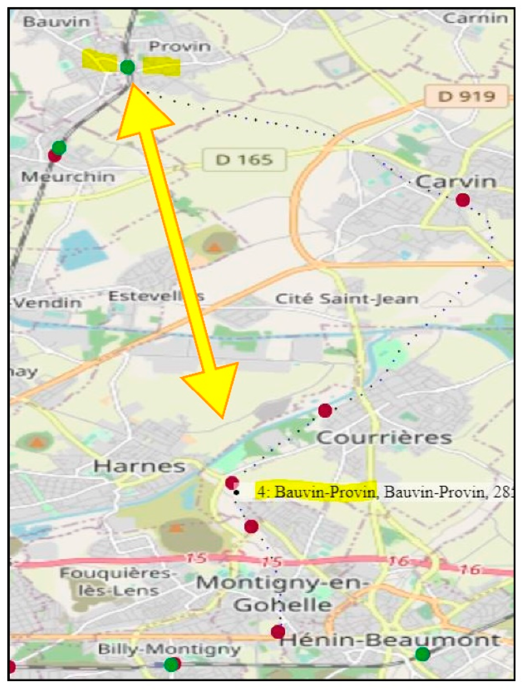
The case Bauvin-Provin is also a fork-pattern: a former, partly dismantled ligne, going to that gare, ends then (at recording date) at a forknode, therefore this is the last fork before Bauvin-Provin (see Figure A1). The case of Saintes, mentioned with the duplicates, is also a fork-pattern.
Figure A1.
The Bauvin–Provin “fork-pattern”.

The gare location is on top of the image, between toponyms Bauvin and Provin, the same label in a pop-up print, near the Harnes toponym is explained by the history of the ligne (small blue dots passing through Harnes, Courrières and Carvin).
That lignen°285,000 (ligned’Hénin-Beaumont à Bauvin-Provin) has been closed by segments between 1960 and 1970, and the geometry of the terminus has been attributed twice: (1) the original terminus Bauvin–Provin, was at km = 233.0, (2) then the segment end was near the Harnesgare, at km = 222.39, but with the Bauvin–Provin label, although 11.6 km further.
Let’s use some examples in Table A17, of the suspected false positives (SN) that were mentioned in Section 2.4.2.
Table A17.
Cases for false negatives out of the (2014, 2017) direct pairs (top); and lists (bottom).
Table A17.
Cases for false negatives out of the (2014, 2017) direct pairs (top); and lists (bottom).
| Cause | Label | Dist (m) |  |
SN: label = & dist > 2.2 km | Reims | 2273 | |
| Champdôtre-Pont | 2299 | ||
| Sillé-le-Guillaume | 2342 | ||
| Argentan | 2355 | ||
| Toucy-Ville | 3446 | ||
| Épinal | 3644 | ||
| Fougères | 4964 |
- Question is: Why the same gare names so far away?
In the example of Reims, there are 4 nodes, two being very close (Reims on picture Table A16), one for the North ligne, and the farthest fork (N-E) being 2.273 km away.
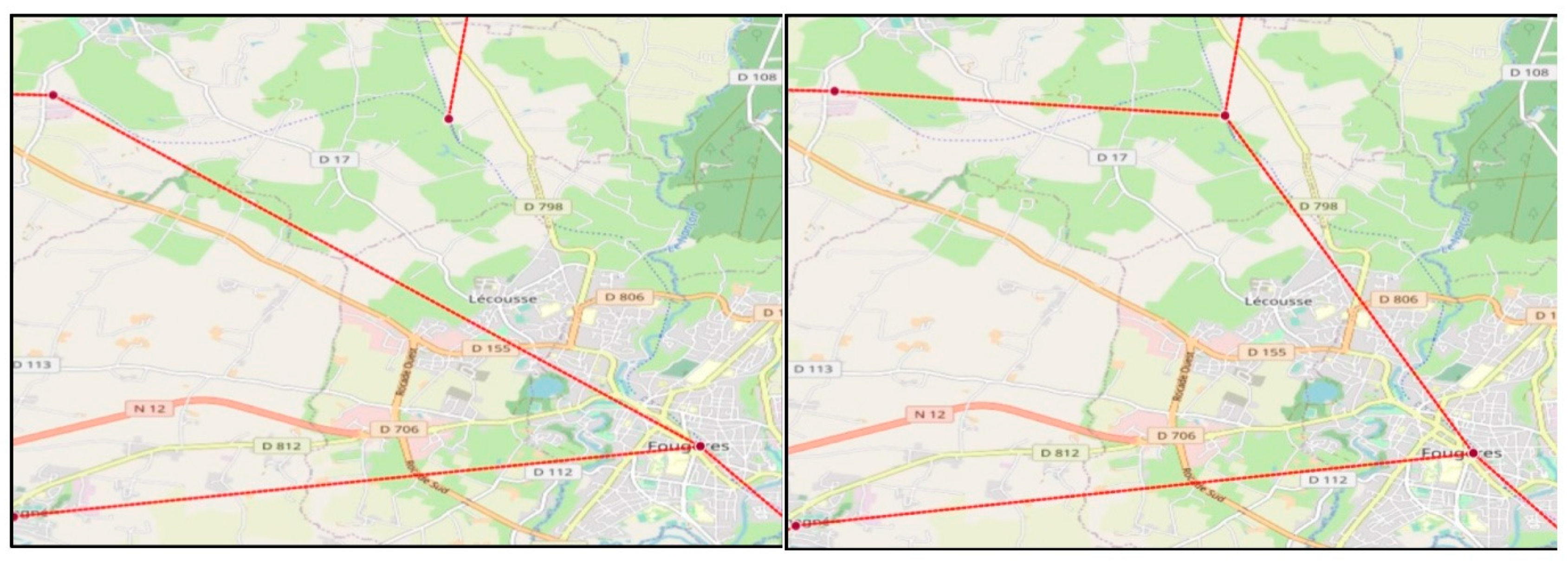
In the example of Fougères (Figure A3, next section), two locations are 4.964 km apart: one is the now a closed gare, the other is the last fork of the former ligne, still located on an active ligne.
All cases in the list (Table A17) result from the fork-pattern. It was right to tag them “suspected negatives”, and to not fusion them with their respective gares.
Appendix B.3. The Target Schema and the Graph Representation of the Network
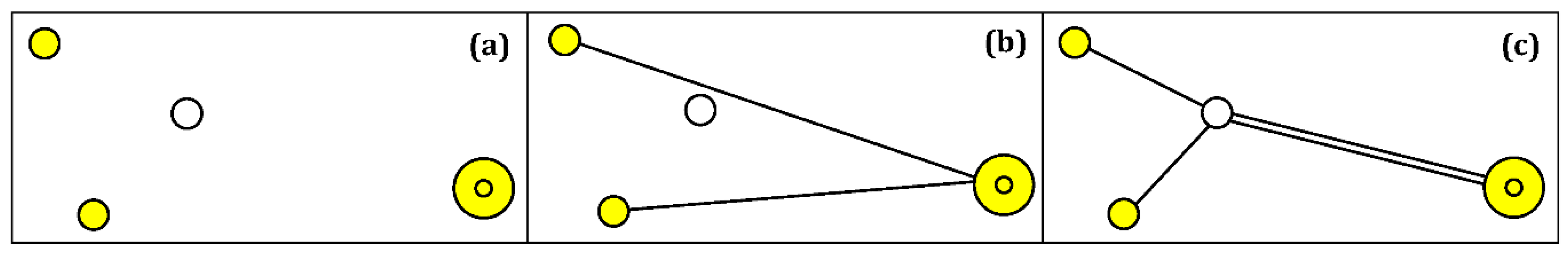
The case with the initial UML-class diagram is that it is does nottake into account correctly the difference between a gare-node, and a non-gare-node, such as a fork. This is not an issue, for instance when confronting gares and communes, which requires a simple “point_in_polygon” algorithm. But a simple example (Figure A2) illustrates the problem: one gare (yellow double circle) is at the junction of two lignes coming from two simple gares (yellow simple circle), and a fork (white circle) gives the exact location of where the two lignes meet (Figure A2-case a).
Figure A2.
Mixing [simple]gare-node, [junction]gare-node and fork-node: (a) no link, (b) links ignoring the forks, (c) links preserving forks.
Figure A2.
Mixing [simple]gare-node, [junction]gare-node and fork-node: (a) no link, (b) links ignoring the forks, (c) links preserving forks.

Case (b): the fork is ignored and a simple “digraph” representation will work correctly with algorithms: shortest-path (well known algorithm also named after Dijkstra), or path-contraction, an algorithm to build the minor graph of the original graph, which ignores intermediate [simple] gares and nodes (not terminus, not junction).
Case (c) is more complex: it preserves the information of the fork, whichleads to a better visual result. With an historical viewpoint, archiving more geographical information about the past network is much better.
The fork-pattern example of Fougères (Figure A3), involves four lignes (N, S-E, S-W, N-W). In the original data, the fork North was the last node in the list, hence plotted as the terminus: this is solution (b), illustrated on the left. Solution (c) is on right.
Figure A3.
Example of the gare of Fougères before and after addition of the fork on ligne North-West.
Figure A3.
Example of the gare of Fougères before and after addition of the fork on ligne North-West.

References
- De Block, G.; Polasky, J. Light railways and the rural–urban continuum: Technology, space and society in late nineteenth-century Belgium. J. Hist. Geogr. 2011, 37, 312–328. [Google Scholar] [CrossRef]
- Martí-Henneberg, J. European integration and national models for railway networks (1840–2010). J. Transp. Geogr. 2013, 26, 126–138. [Google Scholar] [CrossRef]
- Auphan, E. La contraction du réseau ferré français dans le temps et dans l’espace. In Colloque international Le secteur des transports ferroviaires dans la mondialisation; Univ. Versailles-Saint-Quentin-en-Yvelines: Versailles, France, 2013; Available online: https://f-origin.hypotheses.org/wp-content/blogs.dir/2536/files/2015/03/auphan-etienne-atelier-f.pdf (accessed on 14 September 2020).
- Report on implementation of the 2011 EU White Paper on Transport. Roadmap to a Single European Transport Area—Towards a Competitive and Resource-Efficient Transport System. Five Years Later: Achievements and Challenges. 2016. Available online: https://ec.europa.eu/transport/sites/transport/files/themes/strategies/doc/2011_white_paper/swd(2016)226.pdf (accessed on 14 September 2020).
- Siebert, L. Using GIS to Map Rail Network History. J. Transp. Hist. 2004, 25, 84–104. [Google Scholar] [CrossRef]
- Gregory, I.; Ell, P.S. Historical GIS: Technologies, Methodologies and Scholarship; (Cambridge Studies in Historical Geography); Cambridge University Press: Cambridge, UK, 2007; p. 227, (Cambridge Studies in Historical Geography). [Google Scholar]
- Morillas-Torné, M. Creation of a Geo-Spatial Database to Analyse Railways in Europe (1830–2010). A Historical GIS Approach. J. Geogr. Inf. Syst. 2012, 4, 176–187. [Google Scholar] [CrossRef] [Green Version]
- Li, C.; Liu, L.; Dai, Z.; Liu, X. Different Sourcing Point of Interest Matching Method Considering Multiple Constraints. ISPRS Int. J. GeoInf. 2020, 9, 214. [Google Scholar] [CrossRef] [Green Version]
- Normand, S.-L.T. Meta-analysis: Formulating, evaluating, combining, and reporting. Stat. Med. 1999, 15, 321–359. [Google Scholar] [CrossRef] [PubMed]
- Riley, R.D.; Price, M.J.; Jackson, D.; Wardle, M.; Gueyffier, F.; Wang, J.; Staessen, J.A.; White, I.R. Multivariate meta-analysis using individual participant data. Res. Syn. Meth. 2015, 6, 157–174. [Google Scholar] [CrossRef] [PubMed] [Green Version]
- Lan, T.; Longley, P. Geo-Referencing and Mapping 1901 Census Addresses for England and Wales. ISPRS Int. J. Geo-Inf. 2019, 8, 320. [Google Scholar] [CrossRef] [Green Version]
- Bloch, I. Information Fusion in Signal and Image Processing: Major Probabilistic and Non-Probabilistic Numerical Approaches; Wiley- Online Library: Hoboken, NJ, USA, 2008; ISBN 9781848210196. [Google Scholar]
- Benferhat, S.; Kacia, S.; LeBerre, D.; Williams, M.-A. Weakening conflicting information for iterated revision and knowledgeintegration. Artif. Intell. 2004, 153, 339–371. [Google Scholar] [CrossRef] [Green Version]
- Reichgelt, H. Knowledge Representation: An AI Perspective; AblexPublishing: New York, NY, USA, 1991; ISBN 10:0893915904. [Google Scholar]
- Johnson, B.A.; Iizuka, K. Integrating OpenStreetMap crowdsourced data and Landsattime-series imagery for rapid land use-land cover (LULC) mapping: Case study of the Laguna de Bay area of the Philippines. Appl. Geogr. 2016, 67, 140–149. [Google Scholar] [CrossRef]
- Younghoon, K.; Woohwan, J.; Kyuseok, S. Integration of graphs from different data sources using crowdsourcing. Inf. Sci. 2017, 385–386, 438–456. [Google Scholar] [CrossRef]
- Smith, M.J.; Wedge, R.; Veeramachaneni, K. FeatureHub: Towards collaborative datascience. In Proceedings of the IEEE International Conference on Data Science and Advanced Analytics (DSAA), Tokyo, Japan, 19–21 October 2017; pp. 590–600. [Google Scholar]
- Juhász, L.; Rousell, A.; Jokar Arsanjani, J. Technical Guidelines to Extract and Analyze VGI from Different Platforms. Data 2016, 1, 15. [Google Scholar] [CrossRef] [Green Version]
- Chen, Y.; Chen, L.; Zhang, C. CrowdFusion: A Crowdsourced Approach on Data Fusion Refinement. In Proceedings of the IEEE 33rd International Conference on Data Engineering (ICDE), Tokyo, Japan, 19–21 October 2017; pp. 127–130. [Google Scholar]
- Gouvêa, C.; Loh, S.; FortesGarcia, L.F.; Brasil da Fonseca, E.; Wendt, I. Discovering Location Indicators of Toponyms from News to Improve Gazetteer-Based Geo-Referencing. In Proceedings of Brazilian Symposium on Geoinformatics; 2008; pp. 51–62. Available online: http://www.geoinfo.info/portuguese/geoinfo2008/artigos/p13.pdf (accessed on 8 March 2021).
- Hastings, J.T. Automated conflation of digital gazetteer data. Int. J. Geogr. Inf. Sci. 2008, 22, 1109–1127. [Google Scholar] [CrossRef]
- Wikipedia. Route-Diagram. Available online: https://simple.wikipedia.org/wiki/Template:Infobox_rail_line (accessed on 8 February 2021).
- Lange, D.; Böhm, C.; FelixNaumann, F. Extracting Structured Information from Wikipedia Articles to Populate Infoboxes. In Proceedings of the 19th ACM International Conference on Information and Knowledge Management, Toronto, CA, USA, 26 October 2010; pp. 1661–1664. [Google Scholar] [CrossRef] [Green Version]
- Auer, S.; Lehmann, J. What Have Innsbruck and Leipzig in Common? Extracting Semantics from Wiki Content. In The Semantic Web: Research and Applications; Franconi, E., Kifer, M., May, W., Eds.; Lecture Notes in Computer Science; Springer: Berlin/Heidelberg, Germany, 2007; Volume 4519. [Google Scholar] [CrossRef] [Green Version]
- Vasseur, B.; Jeansoulin, R.; Devillers, R.; Frank, A. External quality evaluation of geographical applications: An ontological approach. Fundam. Spat. Data Qual. 2006, 255–270. [Google Scholar] [CrossRef]
- Daniel, F.; Kucherbaev, P.; Cappiello, C.; Benatallah, B.; Allahbakhsh, M. Quality Control in Crowdsourcing: A Survey of Quality Attributes, Assessment Techniques, and Assurance Actions. ACM Comput. Surv. 2018. [Google Scholar] [CrossRef] [Green Version]
- Senaratne, H.; Mobasheri, A.; Ali, L.; Capineri, C.; Haklay, M. Are view of volunteered geographic information quality assessment methods. Int. J. Geogr. Inf. Sci. 2017, 31, 139–167. [Google Scholar] [CrossRef]
- INSPIRE Thematic Working Group Transport Networks. Data Specification on Transport Networks—Technical Guidelines (D2.8.I.7). European Commission Joint Research Centre. April 2014. Available online: https://inspire.ec.europa.eu/id/document/tg/tn (accessed on 8 February 2021).
- Axelsson, P.; Wikström, L. OGC, InfraGML1.0: Part5 Railways—Encoding Standard. 2017. Available online: http://www.opengis.net/doc/standard/infragml/part5/1.0 (accessed on 8 February 2021).
- SNCF Réseaux. Available online: https://ressources.data.sncf.com/explore/dataset/liste-des-gares (accessed on 13 September 2020).
- Auphan, E. L’apogée des chemins de fer secondaires en France: Essai d’interprétation cartographique. Rev. D’histoire Des Chemins De Fer 2002, 24–25, 24–46. Available online: https://journals.openedition.org/rhcf/2028 (accessed on 8 February 2021). [CrossRef]
- SNCF. Available online: https://fr.m.wikipedia.org/wiki/SNCF_Gares_&_Connexions (accessed on 17 August 2020).
- Wikipedia. Available online: https://en.wikipedia.org/wiki/Wikipedia:Route_diagram_template (accessed on 17 August 2020).
- Wikipedia. Available online: https://de.wikipedia.org/wiki/Wikipedia:Formatvorlage_Bahnstrecke (accessed on 8 February 2021).
- Comber, A.; Wulder, M. Considering spatiotemporal processes in big data analysis: Insights from remote sensing of land cover and land use. Trans. GIS 2019, 23, 879–891. [Google Scholar] [CrossRef]
- Sreenivasaiah, P.K.; Kim, D.H. Current Trends and New Challenges of Databases and Web Applications for Systems Driven Biological Research. Front. Physiol. 2010, 1, 147. [Google Scholar] [CrossRef] [PubMed] [Green Version]
- OSM. Available online: https://wiki.openstreetmap.org/wiki/Railway_stations (accessed on 8 February 2021).
- Gervais, M.; Bédard, Y.; Levesque, M.; Bernier, E.; Devillers, R. Data Quality issues and Geographic Knowledge Discovery. In Geographic Data Mining and Knowledge Discovery; Miller, H.J., Han, J., Eds.; 2009; Chapter 5; pp. 99–115. Available online: http://yvanbedard.scg.ulaval.ca/wp-content/documents/publications/518.pdf (accessed on 8 February 2021).
- Yang, S.; Wu, Y.; Sun, H.; Yan, X. Schemaless and Structureless Graph Querying. In Proceedings of the 40th International Conference on Very Large Databases (VLDB); 2014; Available online: https://yinghwu.github.io/mat/papers/Schemaless_and_Structureless_graph_querying-vldb14.pdf (accessed on 8 February 2021).
- Auphan, E.; Dupuy, G. Vingt ans de travaux scientifiques sur les réseaux et la mobilité ferroviaires. Rev. D’histoire Des Chemins De Fer 2009, 39, 95–101. [Google Scholar] [CrossRef]
- Eurostat. Modal Split of Inland Freight Transport. Statistics Explained Website. 2018. Available online: https://ec.europa.eu/eurostat/statistics-explained/index.php?title=File:Modal_split_of_inland_freight_transport,_2018_(%25_share_in_tonne-kilometres).png (accessed on 18 September 2020).
- European Environment Agency. Greenhouse Gas Emissions from Transport in Europe. 2020. Available online: https://www.eea.europa.eu/data-and-maps/indicators/transport-emissions-of-greenhouse-gases-7/assessment (accessed on 8 February 2021).
Figure 1.
Conceptual target schema for communes, gares, lignes and nodes(primary key: bold font).

Figure 2.
an illustration from the INSPIRE railway network standard (excerpted from [28]).
Figure 2.
an illustration from the INSPIRE railway network standard (excerpted from [28]).

Figure 3.
Matching Sncf2014 and Sncf2017.

Figure 4.
Breakdown by 50 m distance intervals: typical shape and best inflection position.

Figure 5.
Decision diagram depending on the distance in fusion-candidate pairs of nodes. Notations: AP:”assumed positive”, PP:”possible positive”, AN:”assumed negative”, PN:”possible negative”, SP:”supposed positive”, SN:”supposed negative”, und:”undecided”.
Figure 5.
Decision diagram depending on the distance in fusion-candidate pairs of nodes. Notations: AP:”assumed positive”, PP:”possible positive”, AN:”assumed negative”, PN:”possible negative”, SP:”supposed positive”, SN:”supposed negative”, und:”undecided”.

Figure 6.
The coordinates of a commune center and its gare (5.31 km apart in that example).

Figure 7.
Infobox for a commune (Ercé). Relevant items underlined (excerpt from screen console).

Figure 8.
Infobox for a gare (Gare de Rennes). Relevant items underlined.

Figure 9.
Infobox_Ligne_ferroviaire with Ligne_d’Audun-le-Tiche_à_Hussigny-Godbrange.

Figure 10.
Top: Infobox sample code (left) and display (right). Bottom: result of processing the Infobox of: ‘Ligne_d’Audun-le-Tiche_à_Hussigny-Godbrange’ (Figure 10).
Figure 10.
Top: Infobox sample code (left) and display (right). Bottom: result of processing the Infobox of: ‘Ligne_d’Audun-le-Tiche_à_Hussigny-Godbrange’ (Figure 10).

Figure 11.
Example of semi-structured input text with list of gares (top); result of the parsing (middle); and resulting geojson list of nodes (bottom).
Figure 11.
Example of semi-structured input text with list of gares (top); result of the parsing (middle); and resulting geojson list of nodes (bottom).

Figure 12.
Website ‘RemonterLeTemps’: geocoding Chantelle (Allier) at roughly 1/20,000, using a 1954 aerial image, and the scanned map (1952). The double arrow shows the gare, the smaller arrow points to a junction of two lignes (the line to Ebreuil makes a bend to the south).
Figure 12.
Website ‘RemonterLeTemps’: geocoding Chantelle (Allier) at roughly 1/20,000, using a 1954 aerial image, and the scanned map (1952). The double arrow shows the gare, the smaller arrow points to a junction of two lignes (the line to Ebreuil makes a bend to the south).

Figure 13.
Some examples where visual geocoding is not obvious.

Figure 14.
Using alternative maps to resolve indecision: there is a “Chemin de la Gare” indication.

Figure 15.
“Bretagne” region full set of gares, on top of OpenStreetMap: green dots are 2020 active gares on green 2018-active lignes; red dots are ‘past’ gares (mostly on rural tramways).
Figure 15.
“Bretagne” region full set of gares, on top of OpenStreetMap: green dots are 2020 active gares on green 2018-active lignes; red dots are ‘past’ gares (mostly on rural tramways).

Figure 16.
“Bretagne”: active gares (small green dots, 2018) on top of active lignes.

Figure 17.
“Bretagne”: disused or past gares, and lignes. Small black circles = forks.

Figure 18.
The meta-analysis: metadata and improved datasets.

Figure 19.
The full revision procedure: 3-steps fusion, integration and reminder.

Figure 20.
The improved revision procedure: Wikipedia querying, integration and reminder.

Figure 21.
The assisted computer-assisted reconstruction procedure (CARP) visual decision to geo-coding nodes.
Figure 21.
The assisted computer-assisted reconstruction procedure (CARP) visual decision to geo-coding nodes.

Figure 22.
the semi-automated CARP-VGI for integrating a new ligne in the network.

Figure 23.
The CARP posterior quality control.

Figure 24.
Quality control after automated identification of a geographic inconsistency (rule 4).

Figure 25.
Display of rail border crossings (bigger dots) North-East of France. Color indicate which border points are presently open (green).
Figure 25.
Display of rail border crossings (bigger dots) North-East of France. Color indicate which border points are presently open (green).

Figure 26.
Internationalization of the Wikipedia-Infoboxes for lignes (left), and gares (right).

Table 1.
Step-by-step generic approach for adding a gare into the reconstructed network.
|
Table 2.
Public data sources for stations: ‘gare’ or ‘node’ features.
| Sncf2020: “Réseau ferré de France”, last update: 2020, accessed: 8 March 2020 url: https://ressources.data.sncf.com/explore/dataset/liste-des-gares/ Schema (geojson) and counts (4148 features, with geometry): {code_ligne, libelle, fret, voyageurs, code_uic, pk, departemen, commune} +{geometry} |
| Sncf2017, orSNCF2: “Réseau ferré de France”, last update: 2017 url: (authors copy) not available anymore since end 2019, Schema (=Sncf2020) and counts (7702 features, only 6812 with geometry): |
| Sncf2014, orSNCF1: “Réseauferré de France”, last update: 2014, accessed: 8 March 2020 https://data.gouv.fr/fr/datasets/gares-ferroviaires-de-tous-types-exploitees-ou-non/ Schema (CSV) and counts (6442 features, all attributes: 6442): [code_ligne, nom, nature, latitude (WGS84), longitude (WGS84)] |
Table 3.
Public data sources for cities and towns: ‘commune’, and railway lines: ‘lignes’.
| Insee-new: official codes for commune (+2003–2021 administrative changes) url: https://www.insee.fr/fr/information/2028028 CSV, counts (35,589 features, 2577 changes in 2018, no geometry) |
| Insee-geo: commune contours (curated by G. David), accessed: 8 March 2020 url: https://france-geojson.gregoiredavid.fr/ geojson, counts (35,798 communes contours with geometry) |
| Lignes: “SNCF Réseau ferré de France”, created: (before 2017), accessed: 8 March 2020 https://ressources.data.sncf.com/explore/dataset/formes-des-lignes-du-rfn/ Schema (geojson) and counts (1779 features, with geometry): {libelle, code_ligne, mnemo}+{geometry} |
Table 4.
Breakdown of distances between the multiple nodes of gares.
| Intervals (nb. Nodes) | [0, 150 m] | [150, 300] | [300, 1 km] | [1 km, 2 km] | [2 km, ∞] |
|---|---|---|---|---|---|
| “Close Enough” | “Rather Far” | ||||
| SNCF2014 (642 nodes/6442) | 550 | 48 | 32 | 6 | 6 |
| SNCF2017 (1360 nodes/7702) | 541 | 184 | 375 | 157 | 103 |
Table 5.
Breakdown of lignes according to their number of nodes.
| Datasets and Link Attribute | Isolated Gare | 2-Gares Ligne | 3 to 7-Gares | 8 to 15-Gares | 16 to 30-Gares | 31 to Max Gares | (Total) |
| SNCF2017 num | 107 | 76 | 245 | 171 | 91 | 44 | 734 |
| SNCF2014 num | 94 | 62 | 191 | 130 | 76 | 40 | 593 |
Table 6.
Initial metadata after meta-analysis of the individual datasets.
| MetadataSncf2014: { “mime”:”csv”, “year”:”2014”, “nbfeatures”:6442, “schema#”: {“label”:6442, “num”:6442, “nature”:6442, “geometry”:6442}, (1) “unos#”: {“label”:6098, “num”:593},”duos#”{“num-label”:6436} (2) } |
| MetadataSncf2017: { “mime”:”geojson”, “year”:”2017”, “nbfeatures”:7702, “schema#”: {“label”:7702, “uic”:7702, “num”:7702, “km”:7702, “capa”:7702, “geometry”:6812}, “unos#”: {“label”:6813, “uic”:6817, “num”:734} } |
(1) notation schema# stands for: count of all occurrences of properties. (2) unos# and duos#: count of unique value occurrence for some properties or couple of properties.
Table 7.
The similarity measures membership to V(x). Dissimilarity measures non membership.
| |y∈V(x)| = |similarNumLabel(x,y)–normalizedShortDistance(x,y)| | (a) |
| similarNumLabel(x, y): (num(y) = num(x)) ∧ (slug(label(y)) = slug(label(x))) → 1 or 0 | (b) |
| normalizedShortDistance(x, y): let d = distanceGreatCircleInMeter(geometry(y), geometry(x)); if (d ≤ D1) → 1; elseif (D1 < d ≤ D2) → (D2 − d)/(D2-D1); elseif (d > D2) → 0 | (c) |
| |y∉V(x)|: |¬similarNumLabel(x,y)–normalizedGreatDistance(x,y)| | () |
| ¬similarNumLabel(x, y): (num(y) ≠ num(x)) ∨ (slug(label(y)) ≠ slug(label(x))) → 1 or 0 | () |
| normalizedGreatDistance(x, y): let d = distanceGreatCircleInMeter(geometry(y), geometry(x)); if (D4 ≤ d) → 1; elseif (D3 < d ≤ D4) → (D4 − d)/(D4 − D3); elseif (D3 > d) → 0 | () |
Table 8.
Breakdown by distance intervals of (2014, 2017) direct pairs; and (2014, 2017) reverse pairs.
Table 8.
Breakdown by distance intervals of (2014, 2017) direct pairs; and (2014, 2017) reverse pairs.
| Intervals | [0, 50 m] | [50, 100] | [100, 150] | [150, 200] | [200, 250] | [250, 300] | [300, 1 km] | [1 km, ∞] |
|---|---|---|---|---|---|---|---|---|
| direct positive | 4618 | 1082 | 375 | 161 | 113 | 72 | 321 | 58 |
| reverse positive | 4501 | 1072 | 348 | 135 | 70 | 48 | 129 | 18 |
Table 9.
(a) From 6979 direct pairs (only those with geometry among 7702). (b) From 6442 reverse pairs (all with geometry).
Table 9.
(a) From 6979 direct pairs (only those with geometry among 7702). (b) From 6442 reverse pairs (all with geometry).
| (a) | ||||||
| intervals | 0–D1 = 150 m. | D1–D2 = 250 m. | D2–D3 = 1000 m. | D3–D4 = 2000 m. | D4–∞. | |
| direct + | 6070 AP: 87.2% | 353 PP: 5.0% | total undecided | ← | 9 SN: 0.1% | |
| direct ¬ | 59 SP: 0.8% | → | 450 und: 6.4% | 18 PN: 0.2% | 25 AN: 0.4% | |
| (b) | ||||||
| intervals | 0–D1 = 150 m. | D1–D2 = 250 m. | D2–D3 = 1000 m. | D3–D4 = 2000 m. | D4–∞. | |
| reverse + | 5944 AP: 91.9% | 251 PP: 3.9% | total undecided | ← | 4 SNs: 0.3% | |
| reverse ¬ | 46 SP: 0.7% | → | 163 und: 2.5% | 4 PN: 0.2% | 30 AN: 0.8% | |
Table 10.
Updated metadata after the revision process (differences with Table 6 are underlined).
Table 10.
Updated metadata after the revision process (differences with Table 6 are underlined).
| MetadataSncf2014: { “mime”:”csv”, “year”:”2014”, “nbfeatures”:6442, “sch#”: {“label” … :6442, “closest”:6442, “fusable”:6189, “integrable”:33} } |
| MetadataSncf2017: { “url”:”g2017”, “mime”:”geojson”, “year”:”2017”, “nbfeatures”:7702, “sch#”: {“label” …:7702, “closest”:6984, “fusable”:6415, “integrable”:41, “coordinates”:6984} } |
Table 11.
Simplified version of an example of Infobox_Ligne_ferroviaire.
| {{Infobox Ligne ferroviaire\n| nomligne = d’Audun-le-Tiche à Hussigny-Godbrange\n| mise en service = 1880\n| fermeture = 1966\n| fermeture2 = 1987\n| numéro = 196000\n| longueur = 8.8\n| écartement = normal\n| … … (more items) … schéma = \n{{BS-table}}\n … {{BSnn}} … series of items describing the nodes along that line (see next Table) … \n{{BS-table-fin}}\n }} |
Table 12.
Simplified version of the BS-table (of the same ligne).
| {{BS-table}} | |
| {{BSbis|…| … … |Ligne d’Esch-sur-Alzette à Audun-le-Tiche}} | |
| {{BS3bis|…| … … |Frontière entre la France et le Luxembourg} | border |
| {{BS5bis|…| … … |Ligne de Fontoy à Audun-le-Tiche}} | |
| {{BS5bis|…| … … |(1) Ligne non déclassée, non exploitée}} | |
| {{BS5bis|…| 21,144|Audun-le-Tiche |(301 m)}} | origin |
| {{BS5bis|…| … … |Ancienne voie vers Villerupt-Micheville}} | |
| {{BSbis|…| 2,4xx| |Bif vers raccordement d’Audun-le-Tiche|}} | branch |
| {{BSbis|…| 4,6xx|Rédange |(340 m)}} | label |
| {{BSbis|…| 5,5xx| |Tunnel d’Adlergrund|(409m)}} | tunnel |
| {{BSbis|…| 6,6xx| |Ancienne frontière France - Empire allemand}} | km |
| {{BS5bis|…| … … |Ligne de Longwy à Villerupt-Micheville}} | |
| {{BSbis|…| 8,8xx|Hussigny-Godbrange |(346 m)}} | branch |
| {{BSbis|..| … … |Ligne de Longwy à Villerupt-Micheville}} | terminus |
| {{BS-table-fin}} |
Table 13.
Some websites about railway lignes and gares in France (short name on the left).
| Archef | http://archeoferroviaire.free.fr accessed on: 8 March 2021 records hundreds of secondary lines, including industrial, military lines, at a high-resolution |
| cdfFR | http://chemindeferenfrance.blogspot.com accessed on: 8 March 2021 gathers cartographic records about a hundred ancient lines |
| GeoCF | http://www.train.eryx.net/hscff/ accessed on: 8 March 2021 records hundreds of secondary lines (in revision) |
| Ligou | https://www.lignes-oubliees.com accessed on: 8 March 2021 “forgotten lines” records 1768 gares and 361 lignes |
| RDrail | http://rd-rail.fr/ by the author of “Les 400 profils des lignes voyageurs du réseau” (2 volumes) |
| Routes | https://routes.fandom.com/wiki/Portail:Transport_ferroviaire_français accessed on: 8 March 2021 several tables about ancient lines, about chronology |
| RuePT | https://rue_du_petit_train.pagesperso-orange.fr accessed on: 8 March 2021 records 6800 street signs mentioning the presence of a former gare (useful for disambiguating precise localization) |
| Traver | http://chemins.de.traverses.free.fr accessed on: 8 March 2021 gathers photographs and cartographic records about ancient lignes |
Table 14.
Example of geocoding queries for gare_de_Cardet (département: Gard).
| Query | [lat,lon] | dist |
|---|---|---|
| ... true coordinates (see: Figure 14 and Section 3.3.3) = | [44.023710, 4.088814] | 0 |
| [lat,lon] = geocode(“gare, Cardet, France”) | [44.026042, 4.081059] | 672 m |
| [lat,lon] = geocode(“rue de la gare, Cardet, France”) | [44.010420, 4.084597] | 1515 m |
| [lat,lon] = geocode(“chemin de la gare, Cardet, France”) | [44.019122, 4.086764] | 536 m |
Table 15.
Comparing breakdown of junction-gares, by distances between their nodes.
| Intervals (nb.Nodes) | [0, 150 m] | % | [150, 300] | [300, 1 km] | [1 km, 2 km] | [2 km, ∞] |
|---|---|---|---|---|---|---|
| 2014 (642 nodes/6442) | 550 | 85.7 | 48 | 32 | 6 | 6 |
| 2017 (1360 nodes/7702) | 541 | 40.0 | 184 | 375 | 157 | 103 |
| CARP (2116 nodes/10,747) | 1418 | 67.0 | 184 | 344 | 115 | 55 |
Table 16.
Comparing breakdowns of nodes according to their count per ligne.
| Datasets | Isolated Gare | % | 2-Gares Ligne | 3 to 7-Gares | 8 to Max- | (Total) |
|---|---|---|---|---|---|---|
| 2014 num | 94 | 15.8 | 62 | 191 | 130 | 593 |
| 2017 num | 107 | 14.6 | 76 | 245 | 171 | 734 |
| CARP num | 50 | 5.2 | 163 | 259 | 486 | 958 |
Table 17.
Communes reached by at least one gare according to public data versions and CARP.
| Sncf2014 (origin 2014) | 5266 | 14.7% | % of the 35,798 communes (updated year-2019) |
| Sncf2017 (origin 2014) | 5279 | 14.7% | |
| Sncf2020 (update 2020) | 3112 | 8.7% | |
| CARP (as of Jan.2021) | 7341 | 20.5% |
Publisher’s Note: MDPI stays neutral with regard to jurisdictional claims in published maps and institutional affiliations. |
© 2021 by the author. Licensee MDPI, Basel, Switzerland. This article is an open access article distributed under the terms and conditions of the Creative Commons Attribution (CC BY) license (http://creativecommons.org/licenses/by/4.0/).
Share and Cite
MDPI and ACS Style
Jeansoulin, R. A Century of French Railways: The Value of Remote Sensing and VGI in the Fusion of Historical Data. ISPRS Int. J. Geo-Inf. 2021, 10, 154. https://0-doi-org.brum.beds.ac.uk/10.3390/ijgi10030154
AMA Style
Jeansoulin R. A Century of French Railways: The Value of Remote Sensing and VGI in the Fusion of Historical Data. ISPRS International Journal of Geo-Information. 2021; 10(3):154. https://0-doi-org.brum.beds.ac.uk/10.3390/ijgi10030154
Chicago/Turabian StyleJeansoulin, Robert. 2021. "A Century of French Railways: The Value of Remote Sensing and VGI in the Fusion of Historical Data" ISPRS International Journal of Geo-Information 10, no. 3: 154. https://0-doi-org.brum.beds.ac.uk/10.3390/ijgi10030154
Note that from the first issue of 2016, this journal uses article numbers instead of page numbers. See further details here.