Applicability Evaluation of Several Spatial Clustering Methods in Spatiotemporal Data Mining of Floating Car Trajectory

Abstract

Spatial analysis is an important means of mining floating car trajectory information, and clustering method and density analysis are common methods among them. The choice of the clustering method affects the accuracy and time efficiency of the analysis results. Therefore, clarifying the principles and characteristics of each method is the primary prerequisite for problem solving. Taking four representative spatial analysis methods—KMeans, Density-Based Spatial Clustering of Applications with Noise (DBSCAN), Clustering by Fast Search and Find of Density Peaks (CFSFDP), and Kernel Density Estimation (KDE)—as examples, combined with the hotspot spatiotemporal mining problem of taxi trajectory, through quantitative analysis and experimental verification, it is found that DBSCAN and KDE algorithms have strong hotspot discovery capabilities, but the heat regions’ shape of DBSCAN is found to be relatively more robust. DBSCAN and CFSFDP can achieve high spatial accuracy in calculating the entrance and exit position of a Point of Interest (POI). KDE and DBSCAN are more suitable for the classification of heat index. When the dataset scale is similar, KMeans has the highest operating efficiency, while CFSFDP and KDE are inferior. This paper resolves to a certain extent the lack of scientific basis for selecting spatial analysis methods in current research. The conclusions drawn in this paper can provide technical support and act as a reference for the selection of methods to solve the taxi trajectory mining problem.

1. Introduction

Taxi trajectory data possess the characteristics of wide coverage, high sampling density, high position accuracy, large data scale, and rich information [1], and have become the main data set for floating car trajectory research [2,3]. Taxis are generally equipped with GPS receivers, which can record the trajectory points of the taxi movement at regular intervals. The trajectory point includes spatiotemporal information, such as latitude and longitude coordinates, the recording time of the current trajectory point, and this spatiotemporal information is widely used in related research. However, due to the complexity and the large scale of the trajectory data, it is necessary to use appropriate analysis methods to mine the hidden information [4,5].

The research of vehicle trajectory spatial analysis method is very extensive. However, the current research lacks scientific basis for the selection of methods. When solving practical problems, different methods have different characteristics, such as whether parameters need to be set and whether noise points can be eliminated. Therefore, the results obtained may be different and may have a greater impact on the conclusion. When facing specific problems, it is necessary to clarify the characteristics and applicability of each algorithm to choose the appropriate method, so as to improve the scientific nature of related research.

In trajectory data mining, commonly used methods include cluster analysis and density analysis [6,7,8], both of which follow the Tobler’s First Law of Geography, that is, everything is related to everything else, but near things are more related to each other [9]. The clustering method first measures the similarity between data based on specific criteria (such as distance). Secondly, the similarity divides the spatial data set, so that the entities in the same spatial cluster are as similar as possible, while the entities in different spatial clusters are as different as possible [10,11]. The representative of density analysis is Kernel Density Estimation (KDE), which is a nonparametric method that generates a smooth density surface to analyze the spatial distribution characteristics of the data [12]. Many types of spatial clustering algorithms are widely used in vehicle trajectory [13,14]. In the long-term development process, many classification systems have been formed based on different ideas, such as hierarchical and partitioning methods [15]. Hierarchical classification methods represented by hierarchical clustering mostly involve the structure of graphs and trees [16]. In the research on trajectory points, there is no similar parent–child relationship between them. Therefore, the hierarchical method is less applied in the research of floating car trajectory. Moreover, in the partitioning method, according to the number of citations of representative documents describing some classic clustering algorithms in Google Scholar, it can be seen that the application of KMeans and Density-Based Spatial Clustering of Applications with Noise (DBSCAN) algorithms are more extensive among many clustering algorithms; as of February 16, 2021, KMeans has been cited 12,725 times and DBSCAN has been cited 20,247 times. Among them, the KMeans algorithm is representative of clustering methods based on the distance between trajectory points [17], and the DBSCAN algorithm is a representative clustering method based on the distribution of trajectory points [18]. In recent years, a new clustering algorithm, Clustering by Fast Search and Find of Density Peaks (CFSFDP) has been proposed. Its basic idea is to select cluster centers based on distance and density for clustering, which is a clustering method combining density and distance [19]. The number of citations in Google Scholar shows that this algorithm has been cited a large number of times, showing an upward trend year on year. Therefore, this paper selects the four typical spatial clustering methods mentioned above to explore their applicability to specific problems.

Taxi trajectory contains a large amount of information about population flow and residents’ travel [20,21], and mining the hidden spatial information is also one of the hotspots in the study of taxi trajectory [22,23,24]. At the same time, mining the laws of residents’ travel behavior can also explore the spatial evolution of the city and provide references for urban planning [25,26]. Current research hotspots include discovering the hotspot areas where residents travel [27,28,29], identifying urban functional zoning [30,31], calculating the location of a Point of Interest (POI) and the identification of its status of the entrance [32,33], and the evaluation of the influence of an Area of Interest (AOI) according to the degree of aggregation of trajectory points [34], and so on. When solving problems, the time efficiency of the algorithm is also one of the important indicators to evaluate its applicability. Therefore, this paper applies four typical spatial analysis methods to the hotspot spatiotemporal mining problems of taxi trajectory, such as hotspot discovery, POI position extraction, hotspot classification, and time efficiency, along with experiments to verify the applicability of the spatial clustering method. It provides a clearer scientific basis and reference for selecting research methods related to sliding trajectories, and to a certain extent improves the current situation of indiscriminate use of spatial analysis methods, thereby increasing the depth and breadth of related research.

The main work of this paper includes:

(1)

Set the most appropriate parameters to make the four algorithms achieve the best results, and then apply them to the taxi trajectory points in the study area. We use these four algorithms to extract hotspots, and verify the accuracy through field investigations. Compare the result to evaluate the applicability of these algorithms in hotspots discovery.

(2)

Apply the four algorithms to the taxi trajectory point to extract the entrance type POI, and use the distance from the extracted position to the doorposts on both sides as the error to evaluate the applicability of the algorithm in the entrance type of POI position extraction.

(3)

Classify the heat of hotspots in the sample area, verify with Baidu city heat map (https://map.baidu.com/, accessed on 3 March 2021), and evaluate the applicability of the algorithm in the hotspot classification.

(4)

Set the optimal parameters to minimize the influence of the parameters on the running time of the algorithm, apply the four algorithms to different numbers of trajectory points, and compare the running time to evaluate the applicability of the algorithm in the time efficiency.

2. Materials and Methods

There are many spatial analysis methods, among which cluster analysis and density analysis are commonly used methods. This paper applies four typical spatial analysis methods to taxi trajectory data to explore their applicability in different scenes. This section will introduce the data and methods used in this paper in detail.

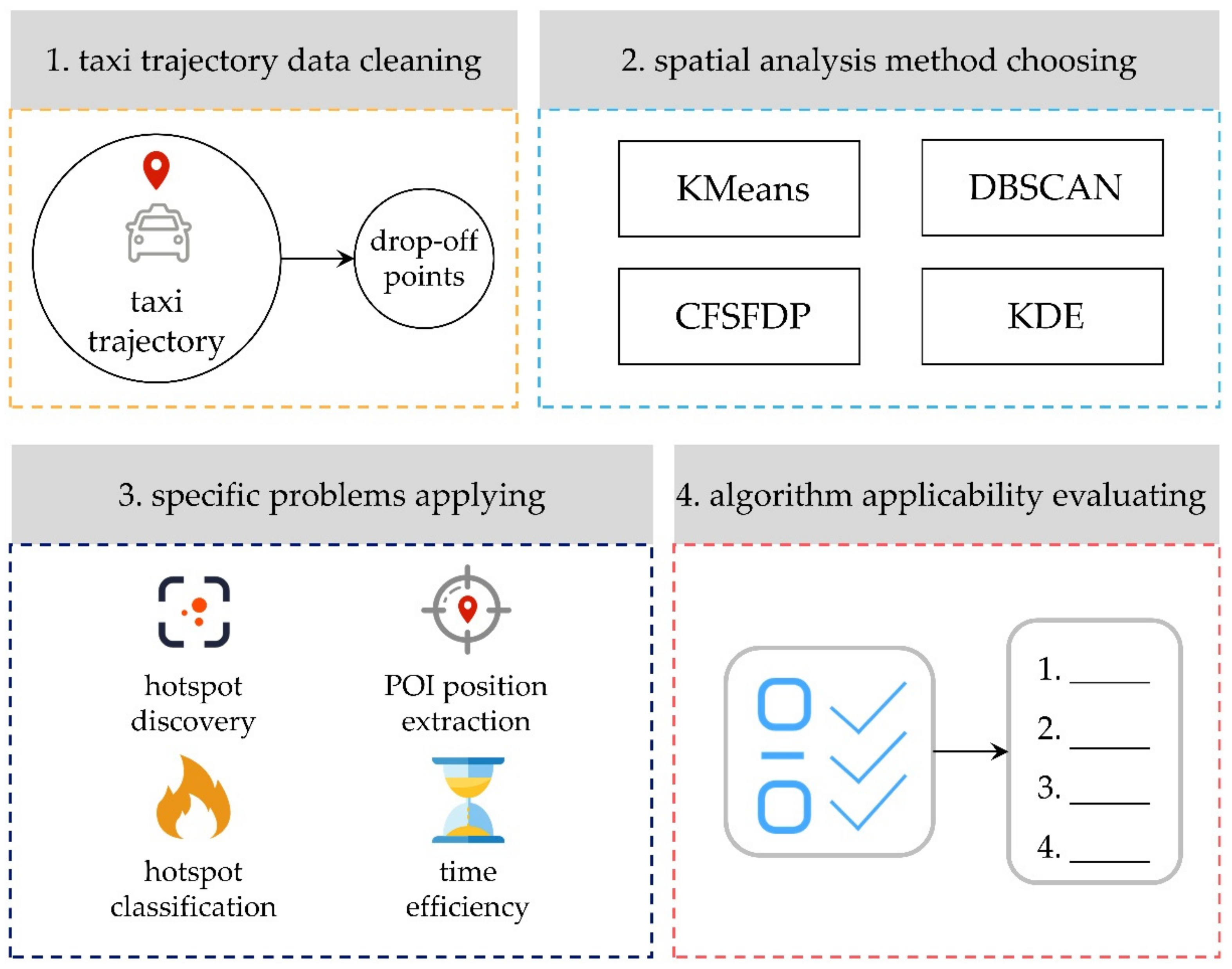
2.1. Research Framework

(1)

First, remove the empty data in the taxi trajectory points, and then extract the drop-off points from them and clean the data points with obvious spatial errors. Using the cleaned data for subsequent experiments can help improve the accuracy of the experiment.

(2)

Select a spatial analysis method and analyze the distribution of taxi drop-off points in the sample area.

(3)

Analyze the effect of the algorithm in solving specific problems through experiments.

(4)

Explore the applicability of each algorithm in different scene based on the experimental results.

Figure 1 illustrates the research framework and methods used in this paper, with the detail given below.

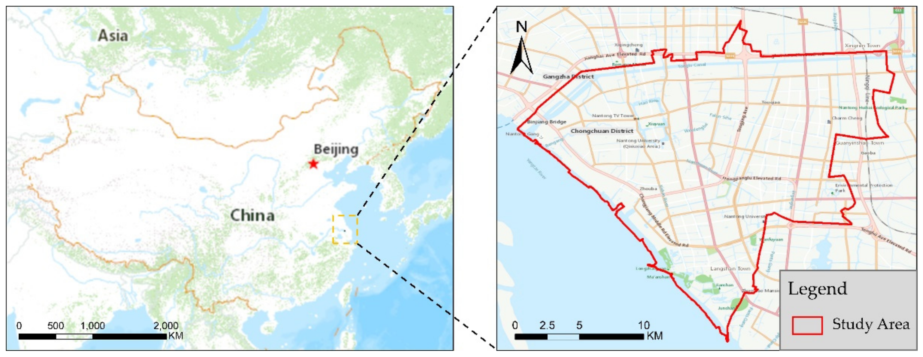
2.2. Study Area

The research area for this paper is shown in Figure 2. All experiments were conducted in Chongchuan District, Nantong City. Nantong City is a prefecture-level city in Jiangsu Province, of which Chongchuan District is the main urban area of Nantong City, with a total area of about 139 square kilometers. As Nantong City has not yet built a subway, and shared bicycles have not been popularized, the main public transportation methods for Nantong residents are taxis and buses. The total number of taxis is about 1200, and the total number of buses is about 3000.

2.3. Taxi Trajectory Data

Taxi trajectory data consist of continuous trajectory points: the set T = {${\mathrm{P}}_1$, ${\mathrm{P}}_2$ … ${\mathrm{P}}_n$}, where ${\mathrm{P}}_n$ is the trajectory point and n is the number of trajectory points. The on-board GPS collects trajectory point information every 30 s, including Plate Number, Phone Number, Time, Latitude and Longitude, Speed, Direction, and Passenger Status; the original data is shown in

Table 1. Original trajectory data.

Plate Number	Phone Number	Time	Latitude and Longitude (°)	Speed (km/h)	Direction	Passenger Status
Su FB3451	136****4156	2018/10/1 0:00	120.908617,31.976048	0	east	1
Su FB3451	136****4156	2018/10/1 0:30	120.911718,31.976479	25.3	east	0
⋮	⋮	⋮	⋮	⋮	⋮	⋮
Su FB3451	136****4156	2018/10/1 23:30	120.859515,32.011984	0	east	1
Su FB3451	136****4156	2018/10/2 0:00	120.859876,32.016244	18.1	northeast	1

.

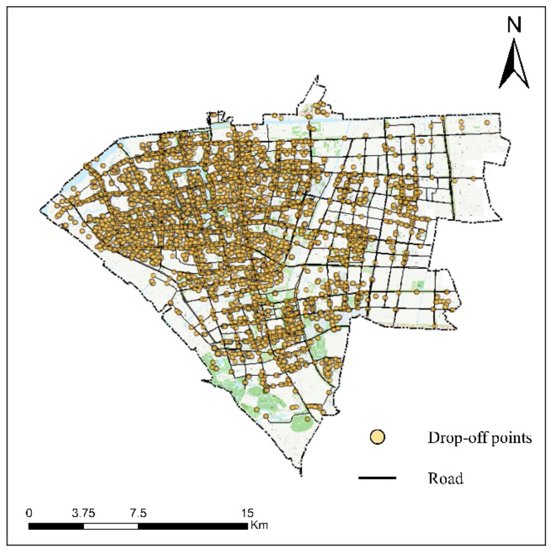
The passenger status indicates whether the vehicle is carrying passengers, 0 means there are no passengers, and 1 means there are passengers in the car. When the passenger status at trajectory point ${\mathrm{P}}_i$ to ${\mathrm{P}}_{i+1}$ changes from 0 to 1, it means point ${\mathrm{P}}_{i+1}$ is the drop-off point. Because some drivers stop pricing before reaching their destination, the recorded drop-off point is not accurate. This paper based on the trajectory data of 1000 taxis in Nantong City in October 2018. In October, ordinary working days, weekends, and National Day holidays are included, which makes trajectory data rich in types, covering a variety of travel purposes. The drop-off points with obvious spatial location errors are first removed, and then the drop-off points with a distance greater than 50 m from the previous record point are removed. Finally, we extracted 801,679 drop-off points for follow-up research.

The experimental sample area in this paper is Chongchuan District, one of the main urban areas of Nantong City, which contains various functional zones such as scenic spots, schools, hospitals, and shopping malls. The sample types are rich and a large number of taxi drop-off points are gathered, as shown in Figure 3.

2.4. Spatial Analysis Method

The purpose of comparing the pros and cons of the algorithms is to select their optimal parameters. When the spatial clustering algorithm is applied to the taxi trajectory, the clustering results with different parameters are also different. Therefore, to obtain better clustering results, a suitable algorithm with reasonable parameters should be configured. This paper configures the corresponding parameters of the four algorithms according to different scenes and compares the results, so as to explore the application of the spatial clustering algorithm to taxi trajectory research.

2.4.1. KMeans

The KMeans algorithm needs to set the parameter k and divide the data set into k clusters according to the parameters. It first selects k cluster centers, then calculates the distance from each data point to the them, and assigns each point to the closest cluster center until the sum of squares due to error (SSE) is the smallest. The best parameter value is usually determined by the elbow method [35,36], with the k as the horizontal axis, and the SSE as the vertical axis. Observe the mutation point to determine the best k value. The square deviation within the group is calculated as shown in Formula (1).

$$\mathrm{SSE} = {{\displaystyle \sum }}_{j=1}^{\mathrm{K}}{{\displaystyle \sum }}_{z\in {\mathrm{C}}_j}{\left|{z-\mathsf{\mu }}_j\right|}^2$$

(1)

where ${\mathsf{\mu }}_j$ is the cluster center of each cluster, ${\mathrm{C}}_j$ is the number of objects in each cluster, and z is the object in each cluster.

2.4.2. DBSCAN

The DBSCAN algorithm needs to set the radius Eps and the minimum number of samples MinPts. When the radius Eps is selected, the distances from all sample points to the i-th point can be arranged in descending order and a curve graph is drawn. A more reasonable Eps value is the distance from the mutation point to the sample point. The minimum sample number MinPts is usually set through experience to obtain better clustering results.

In clustering, this method can eliminate the influence of noise points and can find clusters of arbitrary shapes. This algorithm divides data points into the following three types:

(1)

Core points: points with the number of objects in the radius Eps more than the minimum number of samples MinPts.

(2)

Boundary points: points with the number of objects in the radius Eps is less than or equal to the minimum number of samples MinPts. Meanwhile, this point is within the neighborhood of the core point.

(3)

Noise point: a point that is neither a core point nor a boundary point.

At the same time, there are the following relationships between points and points in the algorithm:

(1)

Direct density: if point P is the core point, and Eps is the radius as its neighborhood, and Q is in this range, it is said that the density from point P to point Q is direct.

(2)

Density reachable: if there are core points ${\mathrm{P}}_1,{\mathrm{P}}_2,{\mathrm{P}}_3\dots {\mathrm{P}}_n$, the density of ${\mathrm{P}}_{n-1}$ to ${\mathrm{P}}_n$ is direct, and the density of point ${\mathrm{P}}_n$ to point Q is direct, then the density of point ${\mathrm{P}}_n$ to point Q is called density reachable.

2.4.3. CFSFDP

The basic idea of the CFSFDP algorithm is to find higher-density areas surrounded by lower-density areas.

The algorithm needs to set the parameter cutoff distance $d_c$. It first calculates the local density ${\rho }_i$ and distance ${\delta }_i$ of each data point. Then use the local density as the horizontal axis and the distance as the vertical axis to draw the decision diagram. Among them, the calculation formula of local density ${\rho }_i$ and distance ${\delta }_i$ is shown in Formulas (2)–(4).

$${\rho }_i={\displaystyle \sum }_j\chi \left(d_{ij}-d_c\right)$$

(2)

$$\mathsf{\chi }\left(x\right)=\left\{\begin{array}{c}1,\hspace{1em}x\le 0\\ 0,\hspace{1em}x>0\end{array}\right.$$

(3)

$${\delta }_i=\left\{\begin{array}{c}\min \left(d_{ij}\right),\hspace{1em}{\rho }_j>{\rho }_i\\ \max \left(d_{ij}\right),\hspace{1em}{\rho }_j<{\rho }_i\end{array}\right.$$

(4)

where $d_{ij}$ is the distance between point i and point j, and $d_c$ is the cutoff distance.

One of the shortcomings of the CFSFDP algorithm is that the parameters $d_c$ are difficult to determine and usually need to be selected manually based on experience. Therefore, the parameters of the CFSFDP algorithm in this paper are set separately according to the requirements of different scenes.

2.4.4. KDE

Kernel Density Estimation (KDE) converts the data points in the study area into a continuous surface representing density through a kernel function, that is, a raster form [37]. In this algorithm, two parameters need to be set, the kernel function and the bandwidth h, and the kernel function has a small influence on the result [38]. The kernel function selected in this paper is a quartic function.

The bandwidth reflects the overall smoothness of the data point distribution predicted by KDE. The larger the bandwidth, the more obvious the difference between the predicted data point distribution in hotspots and non-hotspots. The bandwidth in the paper is selected based on the “Silverman empirical rule” [39] bandwidth estimation formula, which is applicable to two dimensions, namely, the longitude and latitude of the coordinate point. This method can better reduce the influence of trajectory points that are too far away from the rest of the trajectory points. The calculation method is shown in Formulas (5) and (6).

$$\mathrm{h}=0.9*\min \left(\mathrm{SD},\sqrt{\frac{1}{\ln \left(2\right)}}*\mathrm{D}\right){*n}^{-0.2}$$

(5)

$$\mathrm{SD} = \sqrt{\frac{{{\displaystyle \sum }}_{i=1}^n{\left({\mathrm{x}}_i-\mathrm{X}\right)}^2+{{\displaystyle \sum }}_{i=1}^n{\left({\mathrm{y}}_i-\mathrm{Y}\right)}^2}{n}}$$

(6)

where D is the median of the distance from each trajectory point to the center point, $x_i$, $y_i$ are the longitude and latitude of the trajectory point $P_i$, X and Y are the longitude and latitude of the center point, and n is the number of trajectory points.

2.4.5. Characteristics of Spatial Analysis Methods

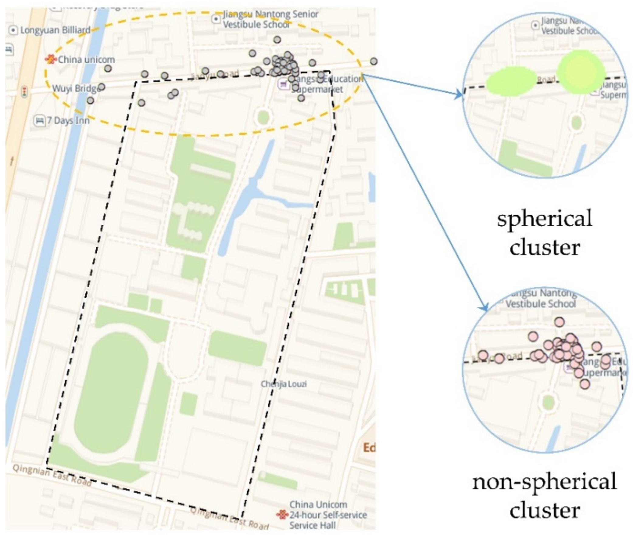
The four spatial clustering algorithms selected in this paper have their own characteristics. Among them, the DBSCAN and CFSFDP algorithms can eliminate the influence of noise points and can find non-spherical clusters. Meanwhile, the KDE and KMeans algorithm is not sensitive to noise points and can only find spherical clusters, as shown in

Table 2. Characteristics of four clustering methods.

Algorithm	Need Parameters	Can Handle Noise Points	Can Non-Spherical Clusters Be Found
KMeans	Yes	No	No
DBSCAN	Yes	Yes	Yes
CFSFDP	Yes	Yes	Yes
KDE	Yes	No	No

Note: In Table 2, DBSCAN refers to Density-Based Spatial Clustering of Applications with Noise, CFSFDP refers to Clustering by Fast Search and Find of Density Peaks, KDE refers to Kernel Density Estimation.

.

3. Results

This section introduces the experiment conducted and the parameter setting method of each algorithm in the experiment. The premise of comparing the applicability of the algorithms is that each algorithm has achieved the best results. When all algorithms have set the optimal parameters, the optimal result can be obtained. This paper combines the experimental results with theoretical analysis and explores the applicability of each algorithm in the four established problems. Since the four spatial analysis methods selected in this paper are all unsupervised methods, there is no need to set training samples. The test data set and verification methods used in each scene are shown in the

Table 3. Sample data and verification methods in each scene.

Scene	Test Data Set	Evaluation Method
Hotspot discovery	drop-off points in the sample area	Field inspection to verify accuracy
Point of Interest (POI) position extraction	drop-off points associated with Are of Interest (AOI)	Compare the error with the actual position
Hotspot classification	drop-off points in the sample area	Use Baidu city heat map to verify accuracy
Time efficiency	A preset number of drop-off point data sets	Compare running time

.

3.1. Hotspot Discovery

The discovery of hotspots is an area of concern in geographic research. In the related research of trajectory data mining, it is usually expressed as an area with a large flow of people and high data density. The drop-off points in the trajectory are usually gathered near the destination of passengers, so the cluster of drop-off points is probably a hotspot [40,41].

Refer to the paper [32] to set the DBSCAN algorithm parameters. Since the study area studied in this paper is larger than the paper [32], the radius Eps and the minimum number of samples MinPts are appropriately enlarged. The CFSFDP algorithm parameters $d_c$ and Eps both represent the search radius, so their settings are the same. After experiments, it is found that when the parameter MinPts of the DBSCAN algorithm is 100, while the clustering result is more consistent with the actual hotspot area distribution. In order to make the number of clustering results of the KMEANS and DBSCAN algorithms the same, we set the parameter k to be the same as the number of clusters in the clustering result of the DBSCAN algorithm. The method of selecting the bandwidth of the KDE algorithm is shown in Formulas (5) and (6) and can reduce the influence of abnormal trajectory points. The optimal parameters of each algorithm in this scene are shown in

Table 4. The optimal parameters of each algorithm in the discovery of hotspots.

Algorithm	Parameter Setting Method
KMeans	K: same number of clusters as DBSCAN algorithm
DBSCAN	Eps: 50, MinPts: 100
CFSFDP	$d_c$: 50
KDE	h: Formulas (5) and (6)

.

This paper selects multiple blocks in Chongchuan District of Nantong City, sets four algorithms according to preset parameters and applies them to the drop-off point data in the sample area. First, divide the experimental plot into multiple blocks according to the road. Randomly select a few blocks, conduct experiments on the drop-off points among them, and add the results to calculate the accuracy. We have verified the accuracy of each algorithm through field inspections, such as calculating the POI density in the area and examining the operating status of related POIs. The accuracy is shown in

Table 5. Verification of the accuracy of hotspot discovery.

Algorithm	KMeans	DBSCAN	CFSFDP	KDE
Number of hotspots found	92	92	34	77
Accurate number	68	87	29	73
Accuracy	73.9%	94.6%	85.3%	94.8%

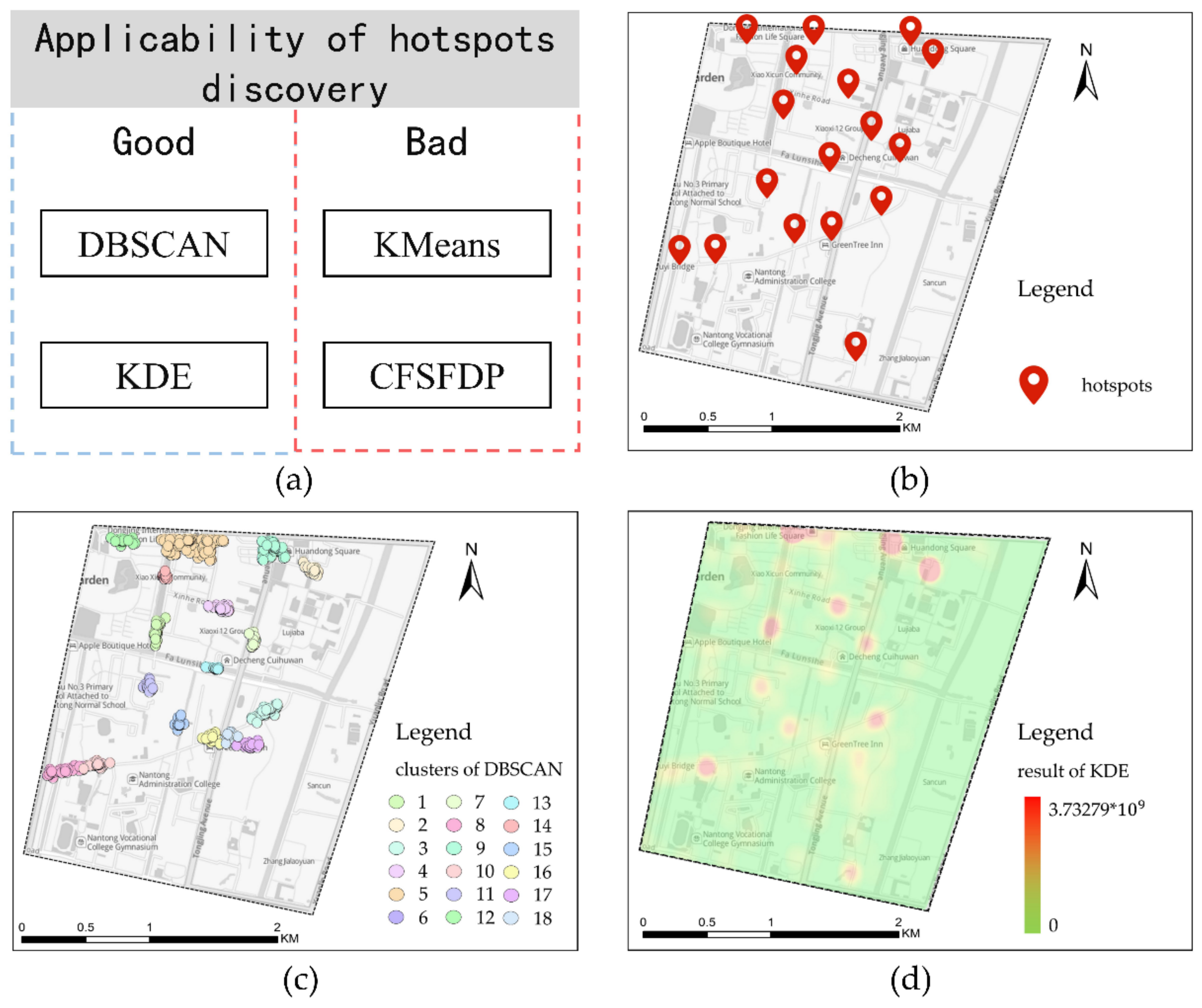
. It can be seen from Table 5 that the hotspots mined by the DBSCAN and KDE algorithms are more in line with the actual situation and more accurate. KMeans and CFSFDP algorithms have low accuracy in mining hotspots, and the number of hotspots that CFSFDP can find is far less than the other three algorithms. Therefore, DBSCAN and KDE algorithms are more usable in this scene.

The applicability of each algorithm in the hotspot discovery scene is shown in Figure 4a. Taking a block as an example, the distribution of hotspots is shown in Figure 4b. Because the DBSCAN and KDE algorithms can display the distribution characteristics of spatial data points based on their density, they can more accurately find hotspots where the drop-off points are gathered, as shown in Figure 4c,d. However, compared with the former, the KDE algorithm can only mine spherical clusters, as shown in Figure 5. Therefore, the shapes of the hotspots found are different from their real shapes, and the effect is poor when mining complex-shaped non-spherical hotspots.

3.2. POI Position Extraction

In the geographic information system, POI is a point representing geographic objects. When mining the spatial position of such points, the influence of other elements should be avoided as much as possible, and errors in the extraction results should be reduced. In this way, the spatial position or area of the POI point can be displayed more clearly. Entrance and exit points are special types of POIs. The method of [32] is used in this paper to extract the entrance and exit points of AOIs, using four spatial analysis methods to extract a variety of typical AOI entrances and exits, including shopping malls, scenic spots, residential areas, schools, and hospitals. The parameter settings of the four algorithms are shown in

Table 6. The optimal parameters of each algorithm in the discovery of the positions of POIs (Points of Interest).

Algorithm	Parameter Setting Method
KMeans	K: elbow method
DBSCAN	Eps: Observe the mutation points of the graph, MinPts:25
CFSFDP	$d_c$:25
KDE	h: Formulas (5) and (6)

. Because most of the street width in the study area is less than 25 m, and the drop-off points are mostly within the range of the road, the parameter $d_c$ of the CFSFDP algorithm is set to 25 m.

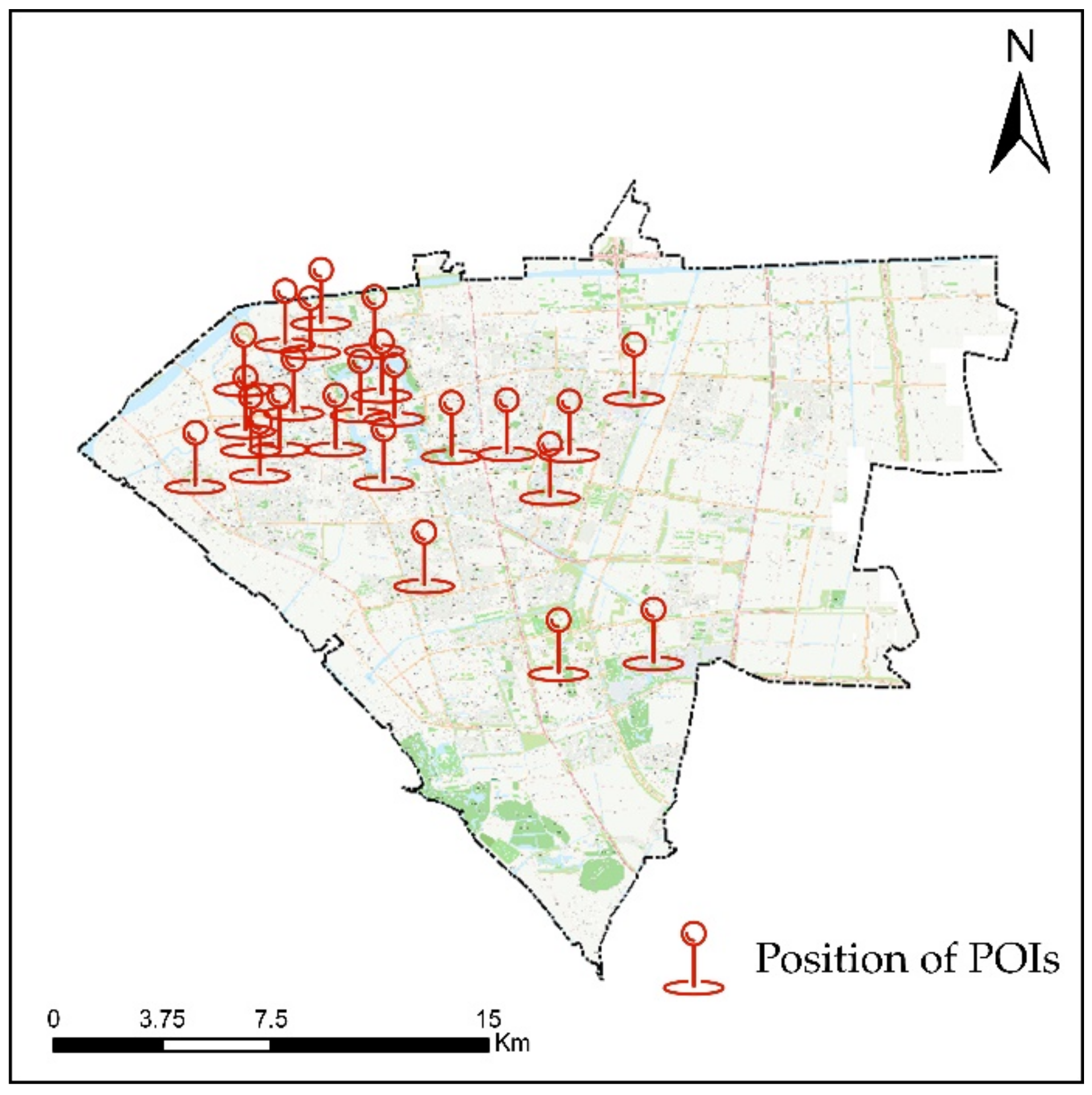
In this paper, a total of 33 entrances and exits are selected in the experimental area, and their position is shown in Figure 6. The extracted entrance and exit positions are compared with the actual ones, and the distance from the extracted position to the doorposts on both sides of the actual entrance and exit is used as the error to evaluate the applicability of the algorithm. The experimental results of various types of AOIs are shown in

Table 7. Average errors in the discovery of the positions of POIs.

Name of AOI	The Extraction Errors of Algorithm (m)
	KMeans	DBSCAN	CFSFDP	KDE
Wuzhou National Square	3.9	0.0	8.0	13.0
Baxian City	0.0	1.3	5.0	6.6
Haohe Museum	12.8	1.9	0.0	0.0
Chunhui Garden	10.0	17.9	1.3	2.0
⋮	⋮	⋮	⋮	⋮
Nantong Vocational University	14.2	3.9	24.8	20.3
Nantong University	0.0	0.0	0.0	3.3
Average Error	15.2	7.3	12.3	18.2

. Among them, the error between the entrance position extracted by the DBSCAN and CFSFDP algorithms and the actual position is 7.3 m and 12.3 m, and the accuracy is high. However, the KDE and KMeans algorithms are not as applicable in this scene as the former two due to larger error in the results.

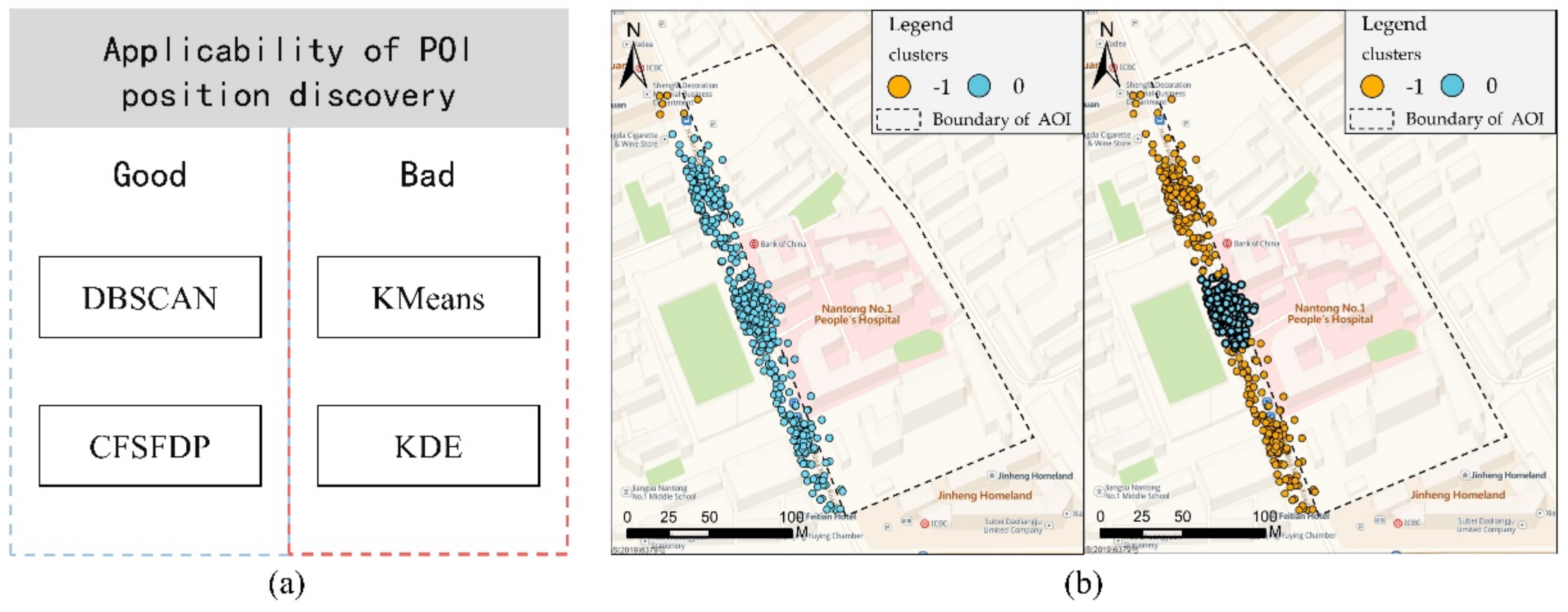
The applicability of the four algorithms in terms of POI position discovery is shown in Figure 7a. Since the spatial location of POI mining requires high accuracy, it is necessary to minimize the influence of abnormal points when performing spatial analysis. The DBSCAN and CFSFDP algorithms cluster drop-off points based on density, which are more sensitive to noise points, and can eliminate the influence of noise points on the results to a certain extent, so they can obtain the higher spatial accuracy requirements of this type of POI.

Although the KDE algorithm can simulate the distribution of trajectory points based on the density, it can find potential special point regions where a large number of trajectory points gather. However, noise points have a greater impact on the KDE algorithm, so this algorithm has poor applicability in the scene where POI locations are found. The KMeans algorithm is similar. Because it is not sensitive to noise points, the extracted POI position has a large error compared with the actual position. In this scene, the spatial accuracy requirement cannot be met, and the applicability is poor.

3.3. Hotspot Classification

Geographical objects usually have their own heat levels. Taxi trajectory points are more likely to cluster around geographical objects with high heat levels. The higher the heat, the more trajectory points there are [42,43]. The clustering results of the drop-off points in the study area in Section 2.1 are classified. The KDE algorithm covers a smooth surface for each trajectory data point, calculates the distribution of data points in its neighborhood, and outputs raster data to represent the study area. That is, pixels organized in rows and columns, each pixel contains a corresponding heat value. The raster data are classified to represent the popularity level of the AOI. The other three algorithms divide the data set into multiple clusters, and judge the level according to the number of trajectory points in the clusters, taking the top three regions of the heat level in each region, and verifying the classification results with the Baidu city heat map (https://map.baidu.com/, last accessed on 3 March 2021). The heat map displays the distribution density of people in the form of heat based on big data of geographic position, so the results of the hotspot classification can be verified. The accuracy of each algorithm is shown in

Table 8. The accuracy of each algorithm in the classification of hotspot.

Algorithm	Accuracy
KMeans	60.0%
DBSCAN	66.7%
CFSFDP	40.0%
KDE	86.7%

.

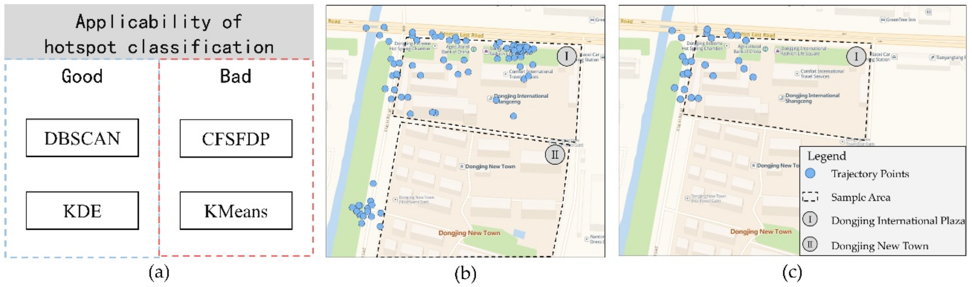
The applicability of the four algorithms for heat grading is shown in Figure 8a. In this sense, the KDE and DBSCAN algorithms are more effective in terms of accurately representing the AOI heat level in the research area. Since the KMeans algorithm clusters drop-off points based on distance, some adjacent AOIs are too close, so they will affect each other during clustering, and will be divided into the same hot area, as shown in Figure 8b. The CFSFDP algorithm searches for points with higher local density in the clustering process. When the data points are more concentrated, multiple high-density core points will be generated. Therefore, some AOIs cannot be completely divided due to the uneven distribution of peripheral trajectory points. In summary, the KMeans and CFSFDP algorithms have a poor applicability on the classification of heat levels.

3.4. Time Efficiency

Among the four spatial clustering algorithms selected in this paper, the parameter setting has little effect on the running time of the algorithm, so this paper uses the best method to set the parameters. The time complexity of the KMeans algorithm is O(ktn), where n is the number of drop-off points, k is the number of clusters, and t is the number of iterations. Since k and t are constants and do not affect the overall time complexity of the algorithm, the time complexity is usually expressed as O(n). However, for the KMeans algorithm, the number of clusters k has a greater impact on its running time. Where the same amount of data and the same number of iterations are used, the more clusters there are, the longer the running time is. According to the elbow method, the optimal parameters of the KMeans clustering algorithm are selected. The k value is concentrated in 2–3, which has little effect on the overall efficiency of the algorithm.

This paper implements four algorithms based on Python 3.7.3 and selects a real data set with 50, 100, 500, 1000, 2000, 5000, and 10,000 drop-off points. Comparing the running time based on the Windows 10 system and a 16GB memory environment, the results are shown in

Table 9. Running time of four algorithms.

Algorithm	Time Complexity	Running Time (ms)
		50	100	500	1000	2000	5000	10,000
KMeans	O(n)	24	43	466	821	1325	6325	18,877
DBSCAN	O(nlogn)	260	610	7550	27,570	106,400	671,610	2,065,351
CFSFDP	O(n2)	1300	6190	150,260	578,920	2,364,070	12,630,400	46,353,924
KDE	O(n2)	823	2659	70,700	292,079	1,116,964	7,233,842	30,246,038

.

It can be seen from Table 7 that, without considering the influence of other parameters, when the amount of data is large, the KMeans and DBSCAN algorithms are more time-efficient. On the other hand, the CFSFDP and KDE algorithms are less time efficient and show poor applicability when the amount of data is too large.

4. Discussion

This paper compares the applicability of the four algorithms in different scenes, and the specific results are shown in

Table 10. Applicability of each algorithm in different scenes.

	Algorithm	KMeans	DBSCAN	CFSFDP	KDE
Scene
Hotspot discovery		*	***	**	***
POI position extraction		*	***	**	*
Hotspot classification		*	**	**	***
Time efficiency		***	**	*	*

* indicates the level of applicability, * indicates poorer, *** indicates better.

. The DBSCAN algorithm uses the longitude and latitude of the trajectory points as characteristic values during clustering. It continuously expands and eliminates noise points according to the connectivity of the clusters. Therefore, it can better divide the data distribution in high density and low density regions. Among the problems related to trajectory points, high-density areas are usually typical areas or key research areas. In this context, the DBSCAN algorithm can better solve practical problems and has strong applicability. Although the KDE algorithm also displays data distribution based on density, it cannot eliminate the influence of noise points. So it has poor adaptability when solving practical problems with a small research area and high precision requirements, such as extracting POI positions. On the contrary, CFSFDP, which can eliminate noise points, is more applicable when solving problems with a small research area, but it is not as applicable as the KDE algorithm when facing problems with a large research area, such as hot spot discovery and heat classification. In terms of time efficiency of the four algorithms, the KDE algorithm and the CFSFDP algorithm involve double loops in the calculation process. So, when the amount of data increases, the time consumed increases significantly, and the applicability is not as good as the KMeans and DBSCAN algorithms.

5. Conclusions

Based on the important issues of the spatiotemporal mining of taxi trajectories, this paper summarizes the applicability of four typical spatial clustering algorithms in hotspot discovery, POI position extraction, hotspot classification, and time efficiency through theoretical analysis and experimental verification. Among them, the DBSCAN and KDE algorithms have higher accuracy in searching hotspots and hotspot classification, and the POI positions extracted by DBSCAN and CFSFDP are more accurate. When processing larger data sets, KMEANS and DBSCAN are more time-efficient.

By comparing the characteristics of the four algorithms, it can be found that whether clustering methods can eliminate noise points when solving practical problems has a greater impact on the results. Because the distribution of vehicle trajectories in real life is quite random, eliminating noise points is more important in trajectory-related research. However, the time efficiency of KMeans clustering is much better than other algorithms when faced with large datasets. Therefore, the amount of data when solving actual problems is also one of the criteria for method selection.

The relevant conclusions drawn in this paper can be directly used as a practical reference for similar research and, at the same time, may be helpful in improving the current situation of low-applicability spatial clustering in this field, providing a clearer standard for the selection of clustering methods and thereby improving the depth and breadth of the related research.