Spatio-Temporal Visual Analysis for Urban Traffic Characters Based on Video Surveillance Camera Data

Abstract

Urban road traffic spatio-temporal characters reflect how citizens move and how goods are transported, which is crucial for trip planning, traffic management, and urban design. Video surveillance camera plays an important role in intelligent transport systems (ITS) for recognizing license plate numbers. This paper proposes a spatio-temporal visualization method to discover urban road vehicle density, city-wide regional vehicle density, and hot routes using license plate number data recorded by video surveillance cameras. To improve the accuracy of the visualization effect, during data analysis and processing, this paper utilized Internet crawler technology and adopted an outlier detection algorithm based on the Dixon detection method. In the design of the visualization map, this paper established an urban road vehicle traffic index to intuitively and quantitatively reveal the traffic operation situation of the area. To verify the feasibility of the method, an experiment in Guiyang on data from road video surveillance camera system was conducted. Multiple urban traffic spatial and temporal characters are recognized concisely and efficiently from three visualization maps. The results show the satisfactory performance of the proposed framework in terms of visual analysis, which will facilitate traffic management and operation.

1. Introduction

With the advent of the era of big data, there has been an explosion in the amount of data in all industries, including transportation. Intelligent transportation system (ITS) is an effective means to improve the performance of urban traffic systems [1]. In recent years, an increasing number of traffic sensing devices (such as video surveillance cameras, loop coils, microwave detectors, etc.) have been deployed on urban roads. These traffic sensing devices collect a great quantity of traffic data, making the intelligent transportation system gradually evolve from technology-driven to data-driven [2,3,4]. The urban road video surveillance camera system generates billions of vehicles monitoring records every year, which contain massive spatio-temporal information of vehicles [5]. These data are stored for an additional 15 days or discarded directly [6]. Road video surveillance camera systems and related data storage devices are expensive to purchase and maintain, but the value of the data they generate has not been effectively utilized [7]. Guiyang is an important regional center city in southwest China, its road video surveillance camera system records more than tens of millions of license plate data every day. Mining urban residents’ traffic characters and travel rules from such an enormous amount of public travel data is of great reference significance for relevant government departments to optimize the road traffic network and formulate involved policies and regulations [8]. On the other hand, display the road traffic status in a more clear and visual friendly visualization map by deep processing of these abstract data resources can greatly improve the utilization efficiency of traffic data, help people intuitively understand urban road traffic conditions and efficiently plan the travel route, which further eases the current urban traffic pressure and traffic congestion. Consequently, it is essential to develop a visualization method for analysis of spatial and temporal characters of urban road traffic.

Existing urban road traffic data visualization technologies include aggregation visualization, direct visualization and feature visualization [9]. Many map service suppliers provide road traffic information visualization functions, such as the thermal diagram function and real-time traffic map. These visualization methods are mostly based on the acquisition of mobile-based stations to locate the number of users in the area [10], and then the map color is rendered by the number of users, instead of using the actual number of vehicles. For example, Baidu thermal map is a big data visualization product launched by Baidu in 2011. The product is based on the location data of mobile phone users on the location-based service platform [11,12,13]. When smartphone users visit Baidu products, the location information they carry will be recorded to form digital footprints. The visualization effect presented by these data mainly reflects the spatial and temporal clustering degree of the urban population but cannot accurately describe the actual situation of vehicle traffic patterns on the road. Moreover, these visualization technologies usually require users to download the application client, but people generally choose to use various tools to get information and browse real-time traffic status through the browser in their daily travel [14]. Even though these technologies provide the user with a browser-based view, they still have drawbacks in terms of efficiency, user experience, and functionality compared to the client products.

Many studies have been conducted on the visual analysis of vehicle spatial and temporal data under the web environment. Several urban road traffic attributes have been recognized through visualization effects from various data sources, such as road network, travel speed, travel volume and traffic congestion [15]. For example, Liu et al. [16] developed a traffic visual analysis method via spatio-temporal graphs, based on records of taxi global positioning system (GPS) devices. Zhang et al. [17] proposed a visualization method of urban hot routes based on license plate number data. These studies provide an effective visual analysis of urban traffic data. However, these methods mainly display road vehicle spatial and temporal traffic trajectories characters, have difficulty in revealing the aggregation characteristics of regional traffic aggregation.

Therefore, this paper aimed at the actual demands of accuracy, authenticity, and ease of use of urban road vehicle traffic data visualized as a map in the network environment. This was combined with computer graphics theory, a spatio-temporal data processing method, visual resource database, and Internet platform development technology, taking license plate data recorded by Guiyang road video surveillance camera system as data support, to systematically study the visualization method of urban road traffic data based on license plate data. Thereby, we presented the general vehicle traffic regulations of the spatial and temporal aggregation characteristics in Guiyang in an accurate and visually friendly way.

The main contributions of this study are summarized as follows:

•

A method for obtaining latitude and longitude data based on address semantic information is proposed.

•

In the process of matching location address information with maps, an algorithm based on outlier detection is developed for eliminating longitude and latitude deviation errors.

•

An urban road vehicle traffic index is designed to quantitatively evaluate the overall operation status of road network traffic.

•

Various friendly interactive visual analytics methods are devised for exploring urban road traffic spatial and temporal characters.

2. Materials and Methods

2.1. Data Sources and Pre-Processing

The visualization of urban road traffic data needs to deal with massive road data, and its accuracy is the basis of experiments [18]. However, traffic data are generally characterized by diversity, randomness and dynamics [19]. Therefore, to eliminate the interference of various uncertain factors and ensure the accurate and real design and completion of urban road traffic data visualization in the web environment, it is necessary to reasonably analyze and process the data recorded by the actual road monitoring system [20]. The data in this paper mainly comes from 13,094,552 license plate data recorded by the Guiyang road video surveillance camera system on 1 October 2018.

The process of data analysis and processing in this article is completed under the MySQL database and R language platform. In the road video surveillance camera data, a monitoring record contains many fields, such as license plate number recognized by the front-end equipment when the vehicle passes the monitoring point; timestamp recognized by the front-end equipment when the vehicle passes the monitoring point; device number responsible for identifying and generating entry monitoring records when the vehicle passes the monitoring point; speed measured by the monitoring equipment when the vehicle passes the monitoring point; access address of the pictures taken and saved by the road monitoring system [21,22,23]; geographic location information of surveillance camera and time when the system monitoring record is stored in the database [24]. Since surveillance camera data contains a variety of feature information, redundancy of information will further affect the accuracy of subsequent visual effects [25]. Therefore, field information in the data that is irrelevant to the visual analysis design needs to be filtered out. The fields used in this article are license plate number recognized by the front-end equipment when the vehicle passes the monitoring point (Hereinafter referred to as the license plate number, LICENCE_PLATE); timestamp recognized by the front-end equipment when the vehicle passes a monitoring point (Hereinafter referred to as the recognize time, RECOGNIZE_TIME) and geographic location information of surveillance camera (Hereinafter referred to as location information, LOCATION_INFORMATION). The data format is shown in

Table 1. Road vehicle license plate data structure.

Fieldname String	Field Type	Example
LICENSE_PLATE	NUMBER(10)	GUI AUD ***
RECOGNIZE _TIME	DATE	2018/10/1 12:02:42 AM
LOCATION_INFORMATION	VARCHAR2(50)	Intersection of Qingxi Road and Guizhu Road

.

2.2. Latitude and Longitude Acquisition

The first step in establishing traffic data visualization is to project geo-location points onto a map. It can be seen from the raw data library content that video surveillance cameras addresses are stored in text description. At present, the commonly used high-level programming language determines the position of point coordinates on the map by longitude and latitude [26]. Therefore, it is necessary to obtain the accurate longitude and latitude information of all geographic information data.

Road surveillance cameras are not distributed at all locations of urban roads. They are generally concentrated at intersections, high-speed entrances, entrances and exits of bridges and tunnels [24,27]. Therefore, 13,094,552 pieces of data in the database does not mean that there are 13,094,552 pieces of address information. Data source libraries are developed and managed in the MySQL database. By filtering address information data through SQL statements, 1063 geographic location sets are obtained. The number of license plates recorded by the monitoring system in unit time is equal to the number of vehicles passing through the point. The number of license plates corresponding to the address information is enumerated, and the geographic location information set with the weight value of the number of vehicles is finally acquired.

Based on the selected 1063 pieces of geographic location information sets, this paper applies R language platform and web crawler technology to obtain the corresponding latitude and longitude coordinate information of the address offered by the map service provider. R language platform has its unique advantages in grasping web information content. The crawler grammar written by it is relatively intuitive and concise, and the rules are more flexible [28]. At the same time, R language can easily handle millions of orders of magnitude of data, and it is a powerful tool for statistical calculation and statistical mapping [29]. By using R language to operate, the data collected from the crawler web page information can be directly used for statistical analysis and data mining, which saves the steps of data re-import or integration.

R language provides RCurl resource package for web crawler technology [30]. The RCurl resource package is an encapsulation of the cURL library (libcurl), enabling some of the functionality of HTTP, such as downloading files from the server, publishing forms, using HTTPS, maintaining connections, reading in binary format, handle redirection, and password authentication [31]. This paper mainly utilized the enc2Native(), URLencode() and readLines() function design algorithm in RCurl resource package to realize fetching the webpage information data. The whole cycle analysis process is as follows:

• Convert the text description address of the data into the encoding required by the URL through enc2Native() function.
• Create an address conversion URL [32], use the URLencode() function to encode strings in a manner suitable for uniform resource location system identifiers for encoding processing.
• Capture the connection object using the getURL() function, read the URL address provided with geographic coordinates in the web API using the readLines() function, parse the results in JSON format [33].
• The Geolocation tool is used to extract the latitude and longitude from the parsed results and store them in the fields that have been created.

With R language and RCurl resource package, the latitude and longitude information of geographical location field in Google map, Baidu map, Tencent map, Bing map and Gaode map were collected respectively. The partial results of longitude and latitude coordinates crawling under R language platform are shown in

Table 2. Partial results of longitude and latitude coordinates.

Location Information	Longitude	Latitude
Intersection of South Sanqiao Road and North Jiaxiu Road	106.6781	26.58608
Bayonet of Sanqiao Overpass	106.6762	26.58659
Intersection of Sanjiang Road and Aerospace Park Road	106.7039	26.50749
Shangmai Toll Station Bayonet	106.5939	26.63491
Xiazhai Road Intersectiont (Bus Station)	106.6717	26.56470
East Exit Expressway (Phase II)	106.7616	26.56996
Intersection of Dongfeng Avenue and Gaoxin Road	106.8204	26.64501
Intersection of Central Zhonghua Road and Provincial Capital Road	106.7189	26.58598
Intersection of North Zhonghua Road and Beijing Road	106.7166	26.60082
Intersection of North Zhonghua Road and Shahe Street (Phase II)	106.7173	26.59842
Intersection of North Zhonghua Road and West Qianling Road	106.7185	26.59248
Intersection of South Zhonghua Road and Zunyi Road	106.7207	26.57788
South Zhonghua Road (Wanguo Edifice) (Phase II)	106.7199	26.57825
South Zhonghua Road Starting Point (Post and Telecommunications Building—Da Nan Gate)	106.7205	26.57861
Intersection of Zhonghua Road and Zhongshan Road	106.7092	26.62991
Intersection of Zhonghua Road and Yan ’an Road (Phase II)	106.7189	26.59147
Intersection of East Zhongshan Road and Fushui Road	106.7215	26.58324
Intersection of East Zhongshan Road and Shidong Road (Phase II)	106.7278	26.58368
Intersection of East Zhongshan Road and Huguo Road (Phase II)	106.7238	26.58371
Intersection of West Zhongshan Road and Central Ruijin Road	106.7122	26.58312
Central Ring Road North (Xiao Guan Tunnel) (Phase II)	106.7033	26.62475
Intersection of Yunfeng Avenue and Middle Ring Road	106.6308	26.68217
Intersection of Yunfeng Avenue and Nanhu Road	106.6307	26.68001
Intersection of North Yuntan Road and West Jinzhu Road	106.6145	26.65848
Intersection of South Yuntan Road and West Xingzhu Road	106.6150	26.62996
Intersection of South Yuntan Road and East Shilin Road	106.6121	26.61759
Intersection of South Yuntan Road and West Guanshan Road	106.6171	26.63990
Intersection of South Yuntan Road and Jinxi Road	106.6126	26.61951
Bageyan Road (Bus Station)	106.7080	26.60136
Intersection of South Park Road and Dusi Road	106.7156	26.57934
South Park Road (Naobaixin Computer Mall)	106.7160	26.58217
Gongyuan Road (Shifu Road-Dusi Road)	106.7166	26.58477
Intersection of Gangyu Street and North Jintang Street	106.7178	26.59822
Yu ’an Tunnel Portal, East Beijing Road (Phase II)	106.7092	26.62991

.

2.3. Latitude and Longitude Precise Method

After obtaining the data of five groups of longitude and latitude coordinate points of address information, this paper utilizes these data to carry out precise calibration, and then visualizes each unique attribute of point data, such as spatial attribute, time attribute and other attributes [34]. Due to the offset error between some latitude and longitude data supplied by the map service provider and the actual location of addresses [35], in order to accurately restore the location of the video surveillance cameras to theirs corresponding road locations, correct and eliminate the influence of longitude and latitude drift on positioning accuracy, it is essential to design algorithm and reduce deviation error.

2.3.1. Map-Matching Algorithm

The existing methods for reconstruction and calibration of latitude and longitude are mainly map matching algorithms. The matching process is classified into two cases according to the sampling property of the data. The first is the point-oriented map matching technology, which includes the matching algorithm based on probability and statistics; the matching algorithm based on D-S evidence theory [36] and the map matching algorithm based on weight [37]. The second is the line-oriented matching technology, which includes the line matching algorithm based on rotational variation metric [38], an algorithm based on iterative multi-resolution trend metric [39], and a matching algorithm based on vehicle driving state and map matching algorithm based on neural network [40]. These matching techniques to eliminate the longitude and latitude deviation generally require multiple groups of continuous GPS trajectory data, such as taxi data or bus data [16,17]. Matching technology corrects deviations via the judgement of trajectory paths. However, the geo-information data in this paper are the longitude and latitude values of multiple map libraries from the same static address, the map matching algorithm mentioned above cannot be adopted.

Given the actual demand for the accuracy of static address latitude and longitude data, this paper utilizes the principle of statistics to design and adopt an outlier detection algorithm. The latitude and longitude data mean of the central trend is extracted, outliers that deviated from most longitude and latitude data due to differences in measuring instruments and geocoding standards are screened and discarded. This algorithm can help eliminate the location drift and inaccuracy of single group of longitude and latitude data and enhance the accuracy of information in the visualization method.

2.3.2. Dixon Detection Method

At present, the common outlier detection algorithms are based on statistics, distance, density, or clustering [41]. For entity data, the method based on probability and statistics is relatively intuitive [42]. The detection methods for abnormal outliers are mainly divided into two categories: consecutive test and block test. Consecutive test is a relatively simple detection method that detects whether one data is abnormal outlier data at a time. Block test is a detection method that can obtain several abnormal outlier values through one test. Regarding the multiple sets of latitude and longitude data in the address geo-information, considering the actual situation, there might be multiple outliers. The block test method with unknown number of outliers is adopted to improve the detection efficiency [43,44,45] To enhance the efficiency and accuracy of the algorithm, the Dixon detection method of outlier detection based on statistics is adopted in this paper.

The Dixon detection method is related to the number of samples, and the variables in the formula change with the number of samples, as shown in

Table 3. Dixon formula table.

$\mathbf{Sample}\mathbf{Size}\mathit{n}$	High-End Anomaly Test Formula	Low-End Anomaly Test Formula
3–7	$D=r10=\frac{X_{\left(n\right)}-X_{\left(n-1\right)}}{X_{\left(n\right)}-X_{\left(1\right)}}$	$D^{\prime }=r^{\prime }10=\frac{X_{\left(2\right)}-X_{\left(1\right)}}{X_{\left(n\right)}-X_{\left(1\right)}}$
8–10	$D=r11=\frac{X_{\left(n\right)}-X_{\left(n-1\right)}}{X_{\left(n\right)}-X_{\left(2\right)}}$	$D^{\prime }=r^{\prime }11=\frac{X_{\left(3\right)}-X_{\left(1\right)}}{X_{\left(n-1\right)}-X_{\left(1\right)}}$
11–13	$D=r21=\frac{X_{\left(n\right)}-X_{\left(n-2\right)}}{X_{\left(n\right)}-X_{\left(2\right)}}$	$D^{\prime }=r^{\prime }21=\frac{X_{\left(2\right)}-X_{\left(1\right)}}{X_{\left(n-1\right)}-X_{\left(1\right)}}$
14–30	$D=r22=\frac{X_{\left(n\right)}-X_{\left(n-2\right)}}{X_{\left(n\right)}-X_{\left(3\right)}}$	$D^{\prime }=r^{\prime }22=\frac{X_{\left(3\right)}-X_{\left(1\right)}}{X_{\left(n-2\right)}-X_{\left(1\right)}}$
$n$ > 30	$D=r22=\frac{X_{\left(n\right)}-X_{\left(n-2\right)}}{X_{\left(n\right)}-X_{\left(3\right)}}$	$D^{\prime }=r^{\prime }22=\frac{X_{\left(3\right)}-X_{\left(1\right)}}{X_{\left(n-2\right)}-X_{\left(1\right)}}$

. In the 1063 address data, each data contains five sets of different longitude and latitude values. Hence, the number of samples in this paper is 5.

The Dixon test method is designed and utilized to detect abnormal outliers. The main steps are as follows:

• Sort the group of data, set the ordered data sequence as $X_1$,$X_2$,$X_3$,$X_4$,$X_5$.
• According to Table 3, calculate the two statistics of this group of data according to the corresponding number of samples, judge the size of the two statistics, and set the larger statistic as $D^{″}$.
• Determine the test level, find the corresponding critical value $D_i$ in the critical value table (

  Table 4. Dixon threshold table.

  No. of Measurements $\mathit{n}$	Significance Level $\partial$
  	$\partial$ = 0.01	$\partial$ = 0.05
  3	0.994	0.970
  4	0.926	0.829
  5	0.821	0.710
  6	0.740	0.628
  7	0.680	0.569
  8	0.717	0.608
  9	0.672	0.564
  10	0.35	0.530
  11	0.709	0.619
  12	0.660	0.583
  13	0.638	0.557
  14	0.670	0.586
  15	0.647	0.565
  16	0.627	0.546
  17	0.610	0.529
  18	0.594	0.514
  19	0.580	0.501
  20	0.567	0.489

  ), and compare it with the relatively large statistic in step 2. If $D^{″}>D_i$ then the corresponding $X_i$ is an abnormal outlier.
• Cycle back to step 1 and continue processing until it is determined that there is no outlier in this group of data, or the number of samples is less than 3. Take the average value of the remaining data to complete the accuracy of longitude and latitude data.

2.3.3. Experimental Verification

Five groups of longitude data corresponding to one geographic location information are randomly selected from the address data library as samples, they are arranged from large to small as: 106.7182; 106.7179; 106.7166; 106.7160; 106.7076. According to the arranged sequence and the formula for detecting outliers in Table 3, the values of $D$ and $D^{\prime }$ are calculated.

$$D=r10=\frac{X_{\left(5\right)}-X_{\left(4\right)}}{X_{\left(5\right)}-X_{\left(1\right)}}=0.785,D^{\prime }=r^{\prime }10=\frac{X_{\left(2\right)}-X_{\left(1\right)}}{X_{\left(5\right)}-X_{\left(1\right)}}=0.037.$$

The significance level is determined to be 0.05 and the critical value $D_n$ is 0.710. According to the judgment rules, when $D$ > $D^{\prime }$ and $D$ > $D_n$, or $D^{\prime }$ > $D$ and $D^{\prime }$ > $D_n$, $X_5$ is determined to be an outlier. The remaining four sets of data continue to be detected, and the values of $D$ and $D^{\prime }$ are calculated.

$$D=r10=\frac{X_{\left(4\right)}-X_{\left(3\right)}}{X_{\left(4\right)}-X_{\left(1\right)}}=0.261,D^{\prime }=r^{\prime }10=\frac{X_{\left(2\right)}-X_{\left(1\right)}}{X_{\left(4\right)}-X_{\left(1\right)}}=0.174.$$

The significance level is determined to be 0.05, and the critical value $D_n$ is 0.829. According to the judgment rule, there is no outlier in this group of data, and the cycle ends. The actual calculation shows that there is one outlier in the five groups of precision data corresponding to the geographic location information. The longitude value after removing the outliers is averaged to obtain the final refined result: 106.717175.

2.3.4. Longitude and Latitude Precision Data Results

Processing of all video surveillance cameras addresses longitude and latitude data, and the optimization algorithm was implemented using the R language programming platform. The precise longitude and latitude data results of 1063 geographic locations in the database are obtained. Part of the data results after precision are shown in

Table 5. Accurate results of partial longitude and latitude data.

Location Information	Longitude	Latitude
Intersection of Qingxi Road and Guichuo Road	106.674136	26.4339128
Niulangguan Toll Station Bayonet	106.736734	26.475621
Intersection of Yuchang Road and West Jiefang Road	106.688973	26.5561462
Intersection of North Yuntan Road and West Jinzhu Road	106.6043572	26.65634893
Intersection of South Yuntan Road and West Xingzhu Road	106.604586	26.62733473
Intersection of South Yuntan Road and East Shilin Road	106.6022091	26.61553349
Intersection of North Jiaxiu Road and Guihuang Highway	106.665456	26.5629167
Intersection of South Jiaxiu Road and Xinqu Avenue	106.661794	26.4989778
Intersection of South Jiaxiu Road and Guizhu Road	106.662373	26.4330015
Intersection of South Jiaxiu Road and Yingbin Road	106.662239	26.4330791
Intersection of Central Baiyun Road and Yunfeng Avenue	106.627956	26.6859182
Intersection of Suocao Road and Jiefang Road	106.72177	26.5657043
Intersection of Jiefang Road and Nanchang Road	106.715209	26.5643663
Intersection of Jiefang Road and Jiarun Road	106.719789	26.5652463
Bayonet of Zazuo Toll Station on Guiyang-Bizhou Expressway	106.707019	26.868088
Intersection of Guizhu Road and Jiangjun Road	106.664953	26.432983
Intersection of East Jinzhu Road and Shibiao Road	106.629514	26.6583566
Intersection of North Jinyang Road and Lincheng East Road	106.619825	26.6489118
Intersection of North Jinyang Road and Jinzhu East Road	106.620301	26.6572878
Intersection of South Jinyang Road and West Xingzhu Road	106.61945	26.6255304

.

2.3.5. Longitude and Latitude Precision Data Results Verification

The accurate longitude and latitude information of some video surveillance cameras’ locations such as the entrances and exits of bridges as well tunnels, highway toll stations and checkpoints can be found according to the database provided by the Public Security Traffic Management Bureau [46]. For the same address, a comparison between the longitude and latitude data obtained by the above algorithm and the longitude and latitude data recorded in the official database from Public Security Traffic Management Bureau is shown in the

Table 6. Longitude and latitude precision data results verification comparison.

Location Information	Longitude (From Precise Algorithm)	Latitude (From Precise Algorithm)	Longitude (From Official Database)	Latitude (From Official Database)
Checkpoint of Guiyang North Toll Station Bayonet	106.668978	26.678813	106.66895	26.67882
Checkpoint of Zazuo Toll Station of Guiyang-Bixi Expressway	106.70702	26.86808837	106.70704	26.86806
Entrance of Daguan Tunnel on Qianlingshan Road	106.6745257	26.61805163	106.67453	26.61806
Checkpoint of Shibanshao Toll Station Bayonet	106.6125618	26.46976894	106.61255	26.46975
Checkpoint of Mengguan Toll Station Bayonet	106.7455599	26.40698916	106.74557	26.40696
Yuan Tunnel Entrance of Beijing East Road	106.7332749	26.59926328	106.73327	26.59925
Checkpoint of Shangmai Toll Station Bayonet	106.5861663	26.63075054	106.58615	26.63075
Guiyang East Exit Expressway Toll Station	106.7390401	26.57226328	106.73902	26.57225
Entrance of Xiaoguan Tunnel on Central Ring North Line	106.6924061	26.62214895	106.69242	26.62215
Military Area South Factory Road Longmen Viaduct	106.7270621	26.55347921	106.72708	26.55350

.

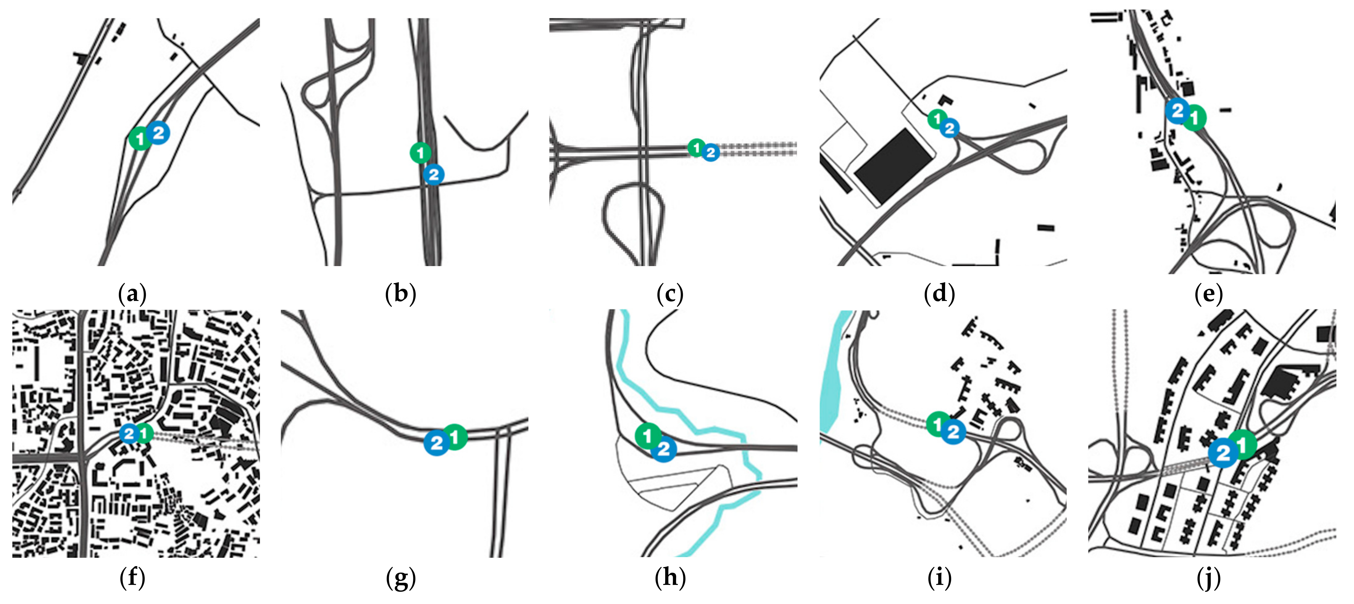
From the comparison between the longitude and latitude data determined by the algorithm and provided by the government, it can be seen that the difference of longitude and latitude is five to six decimal places. When the address information is projected on the map according to two groups of different data, the address points are overlapped on the map, as illustrated in Figure 1, which can prove the effectiveness of the method proposed in this paper.

2.4. Road Capacity Ratio

Road capacity ratio is a road traffic condition detection index based on traffic flow parameters [47]. It can be used as a coefficient to evaluate traffic congestion [48]. Road capacity ratio will change with the passage of time and the change of place (the change of space). According to this characteristic, road video surveillance camera can be utilized to obtain observation relevant data, and then analyze the characteristics and change rules of road capacity ratio in time and space, so as to obtain the basic characteristics of this section of traffic system.

Road capacity ratio refers to the ratio of the actual traffic flow and the maximum traffic flow that the road is designed to withstand. In the equation, $Volume$ represents the actual road traffic flow and $Capacity$ represents the maximum traffic flow limit of road design capacity [49].

$$\frac{V}{C}=\frac{Volume}{Capacity}$$

2.4.1. Traffic Service Level

Traffic capacity ratio is usually measured by traffic service level, as shown in

Table 7. Classification of traffic service level in China.

Service Level	Road Capacity Ratio	Traffic Condition
Level One	<10.4	The traffic flow is stable, basically without delay or a little delay
Level Two	0.4~0.6	Stable traffic flow, with some delays but acceptable
Level Three	0.6~0.75	Close to erratic traffic, with significant delays but tolerable
Level Four	0.75~0.9	Unsteady traffic flow, traffic congestion, delays are unacceptable

and

Table 8. Classification of traffic service level in the United States.

Service Level	Road Capacity Ratio	Traffic Condition
A	<10.4	Smooth traffic flow, basically no delay
B	0.4~0.6	Steady traffic with minor delays
C	0.6~0.75	Close to stable traffic flow, with some delay but tolerable
D	0.75~0.9	Close to unstable traffic flow, with large delay and intolerable
E	0.9~1	Unstable traffic flow, traffic congestion, great delay, unbearable
F	<1	Forced traffic, heavy congestion, stalled traffic

, which compares the difference between road capacity ratio and service level classification in China and the United States [50].

2.4.2. Classification of Location Information of Video Surveillance Camera

The grade of road is divided according to its use function and suitable traffic volume. The grade of roads in different countries is generally similar, but the classification indexes are not identical. Roads in mainland China are divided into five grades: highway, first grade road, second grade road, third grade road and fourth grade road [49]. Urban road video surveillance cameras are distributed on expressways, first grade roads, and second grade roads, as shown in Figure 2 [51].

Expressway is a road with special political significance. It has four or more lanes, with central separation, all grade separation, perfect traffic safety facilities, management facilities and service facilities. It is a multi-lane trunk road for vehicles to drive in different directions and lanes and to control all the entrances and exits. The four-lane expressway can generally adapt to the long-term design of converting various cars into passenger cars, with an average day and night traffic volume of 25,000–55,000. The six-lane expressway can generally adapt to the long-term design of converting various cars into passenger cars, with an average day and night traffic volume of 45,000–80,000. The eight-lane expressway can generally adapt to the long-term design of converting various cars into passenger cars, with an average day and night traffic volume of 60,000–100,000.

First grade road is the road connecting important political, economic and cultural centers and part of the interchange, which is a multi-lane highway for cars to drive in different directions and lanes and to control access according to needs. The four-lane first grade road can generally adapt to the long-term design of converting various cars into passenger cars, with an average day and night traffic volume of 20,000–40,000. The six-lane first grade road can generally adapt to the long-term design of converting various cars into passenger cars, with an average day and night traffic volume of 30,000–60,000.

Second grade road is the main road connecting the political and economic center, or the suburban road with busy transportation. It is a multi-lane road for vehicles. It can generally adapt to the long-term design life of converting various vehicles into passenger cars, with an average day and night traffic volume of 10,000–30,000 vehicles [52,53,54].

2.4.3. Test of the Relationship between Traffic Service Level and Road Capacity Ratio

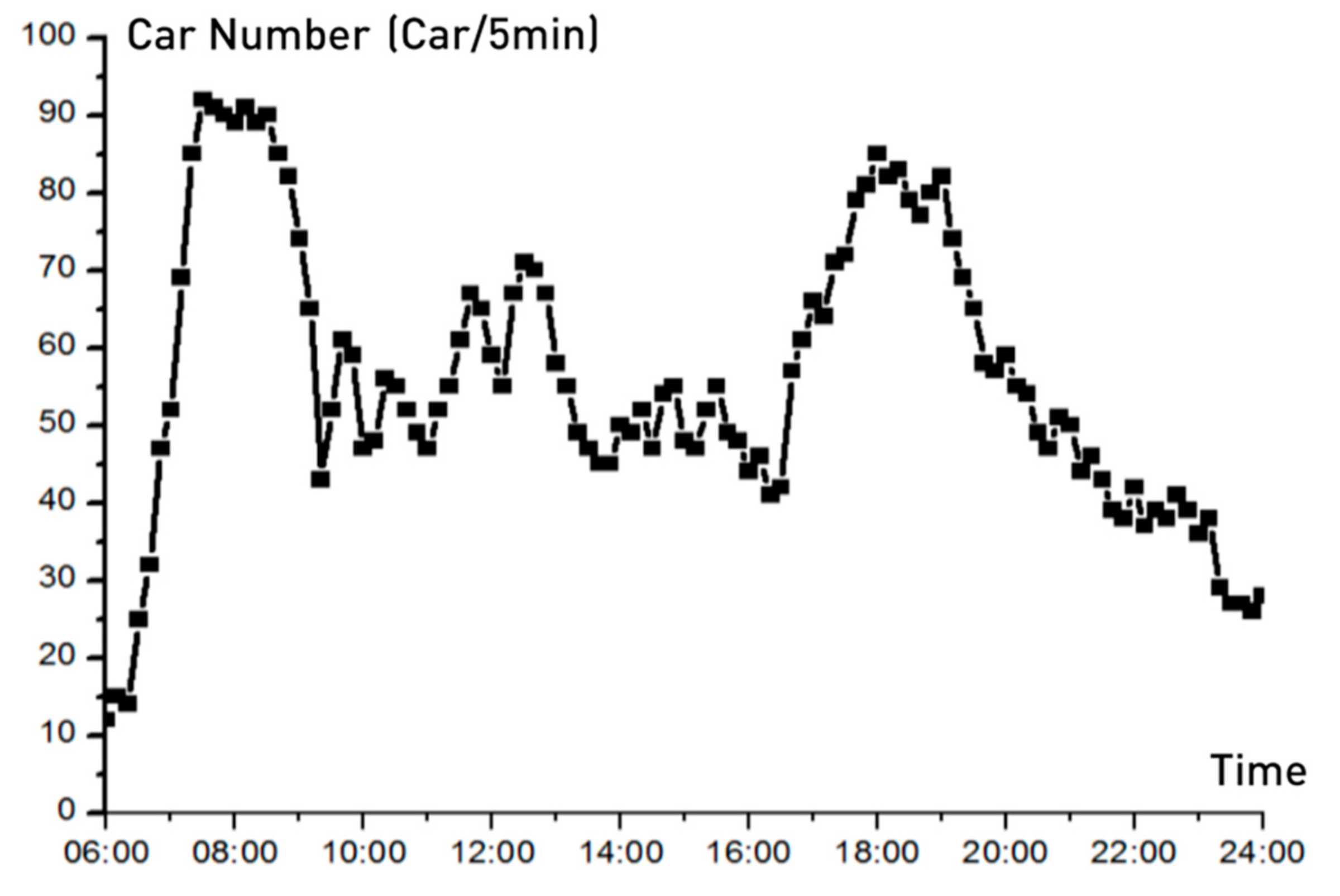
This paper selects East Qianling Road, a four-lane second grade road to verify the detection standard, the maximum traffic flow limit of road design capacity is 30,000, the speed limit on the road is 50 km per hour. According to the road traffic volume data detected by the road video surveillance camera, statistics are made every 5 min to calculate the number of vehicles passing this road Section 5 min before the time to represent the road traffic volume, as illustrated in Figure 3.

In addition, according to the time difference and distance information between multiple surveillance cameras, the average speed of vehicles passing through the road section is obtained, as shown in Figure 4.

By comparing the Figure 3 and Figure 4 and calculating the road occupancy ratio, it can be seen that the traffic condition is related to the traffic volume, and the road occupancy ratio can reflect the urban road traffic situation, the road occupancy ratio corresponding to the road vehicle density on the street is shown in

Table 9. The road occupancy ratio (China Standard).

Car Number (Every 5 Minute)	Road Capacity Ratio	Service Level
10	0.096	Level One
15	0.144	Level One
20	0.192	Level One
25	0.241	Level One
30	0.288	Level One
35	0.337	Level One
40	0.385	Level One
45	0.433	Level Two
50	0.481	Level Two
55	0.529	Level Two
60	0.577	Level Two
65	0.625	Level Three
70	0.673	Level Three
75	0.721	Level Three
80	0.769	Level Four
85	0.817	Level Four
90	0.865	Level Four
95	0.913	N/A
100	0.963	N/A
105	1.001	N/A

and

Table 10. The road occupancy ratio (United States Standard).

Car Number (Every 5 Minute)	Road Capacity Ratio	Service Level
10	0.096	A
15	0.144	A
20	0.192	A
25	0.241	A
30	0.288	A
35	0.337	A
40	0.385	A
45	0.433	B
50	0.481	B
55	0.529	B
60	0.577	B
65	0.625	C
70	0.673	C
75	0.721	C
80	0.769	D
85	0.817	D
90	0.865	D
95	0.913	E
100	0.963	E
105	1.001	F

.

3. Results

3.1. Visualization Map of Urban Road Vehicle Density

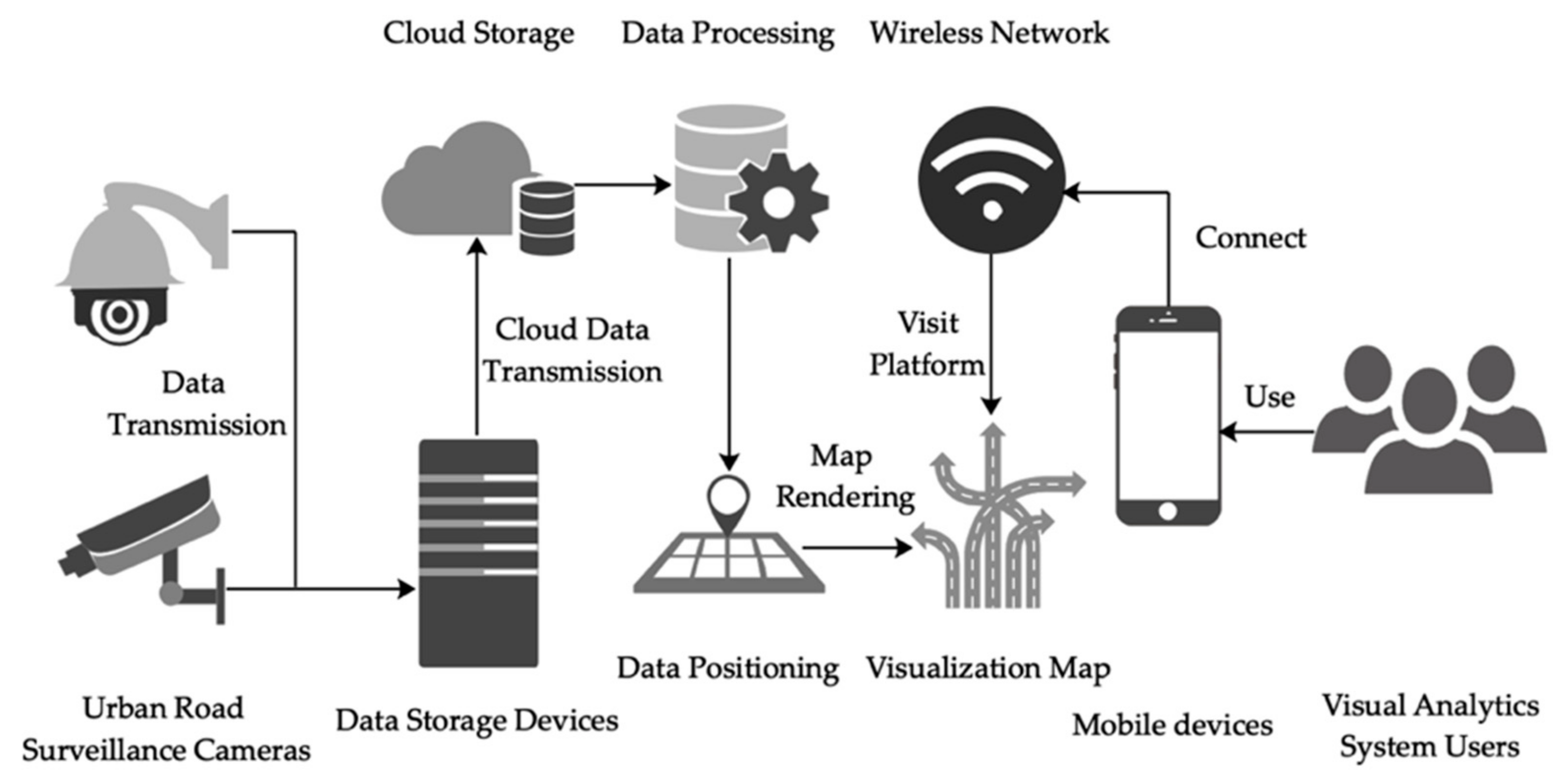
A web-based visual analytics system is developed for end users to explore the spatio-temporal distribution characteristics of urban road vehicles. The visualization system is based on the refined address information data, with the number of license plates captured by surveillance cameras in a unit time as the weight. The interface is designed to comply with the classic visual exploration: Overview first, zoom and filter, details on demand [46].

The visual analytic system was accomplished in JavaScript as a web-based system, the architecture of the system is shown in Figure 5. The system reads geo-information data from the MySQL database, the address geo-information of all 1063 road surveillance cameras in the database are projected to the corresponding positions on a map provided by OpenStreetMap according to latitude and longitude. Conventional map operations such as zooming and dragging are supported. Color transition effect was designed, the vehicle quantity in the corresponding position per unit time is displayed according to the color transition. The number of vehicles corresponding to different colors is displayed below the visualization. End users can set temporal interval, click a location point and obtain the accurate value of the vehicle quantity in this time quantum. As illustrated in Figure 6, the designed visual interface reveals the vehicle density at different road locations in parts of Guiyang from 8:00 a.m. to 9:00 a.m. on 1 October 2018.

3.2. Visualization Map of Urban Regional Vehicle Density

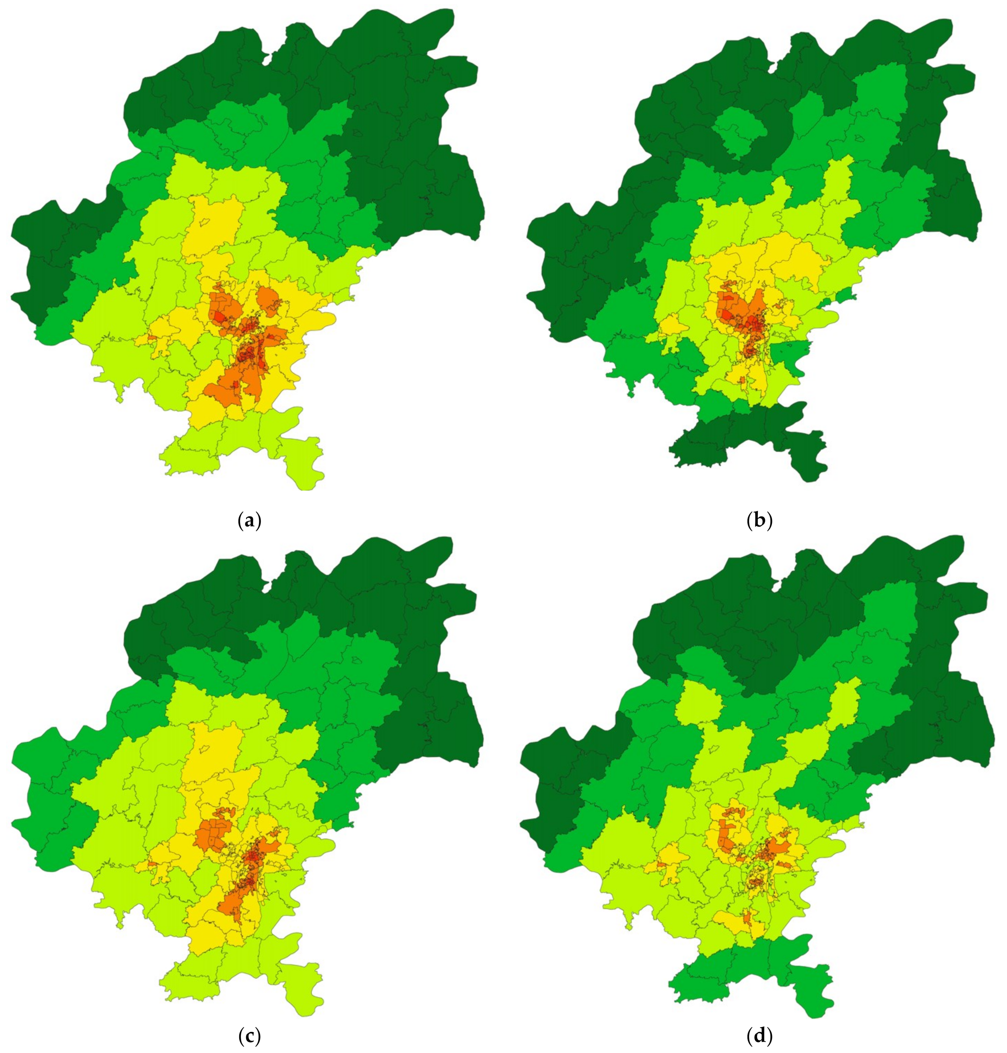
Guiyang has six municipal districts, three counties and one county-level city. There are 32 townships, 45 towns, and 90 communities. According to the scope of administrative divisions of townships, towns and communities in Guiyang provided by the Department of Natural Resources of Guizhou Province, this paper developed a web-based visual analysis system for end users to examine the vehicle density in different areas of the city at diverse times. The regional vehicle density is determined by the average number of license plates captured by all surveillance cameras per unit time in the area.

This paper proposes an urban road vehicle traffic index. The urban road vehicle traffic index is a comprehensive index that quantitatively evaluates the overall operation status of road network traffic. Compared with the traditional speed, flow and other data information, it is intuitive and plain. The urban road vehicle traffic index allows users not only to know whether the traffic is congested vaguely, but also to comprehend the degree of traffic congestion in the whole city and the specific area.

The traffic index consists of six levels: empty; unimpeded; basically unimpeded; slow; slightly congested; congested. The corresponding information of different levels in the urban road vehicle traffic index, such as the number of vehicles passing the detection point in unit time, the images captured by surveillance cameras and the corresponding colors on the map, are shown in

Table 11. Urban road vehicle traffic index information.

Index Level	Color	Road Capacity Ratio	Image
Empty	RGB (3,112,29)	0–0.4
Extreme Low Road Occupancy	RGB (0,182,43)	0.4–0.6
Low Road Occupancy	RGB (186,247,0)	0.6–0.75
Medium Road Occupancy	RGB (247,232,0)	0.75–0.9
High Road Occupancy	RGB (247,128,0)	0.9–1
Extreme High Road Occupancy	RGB (247,58,0)	≤

.

Based on the urban road vehicle traffic index, the visualization map of urban regional vehicle density is designed. End users can set time conditions, zoom and drag the visualization map.

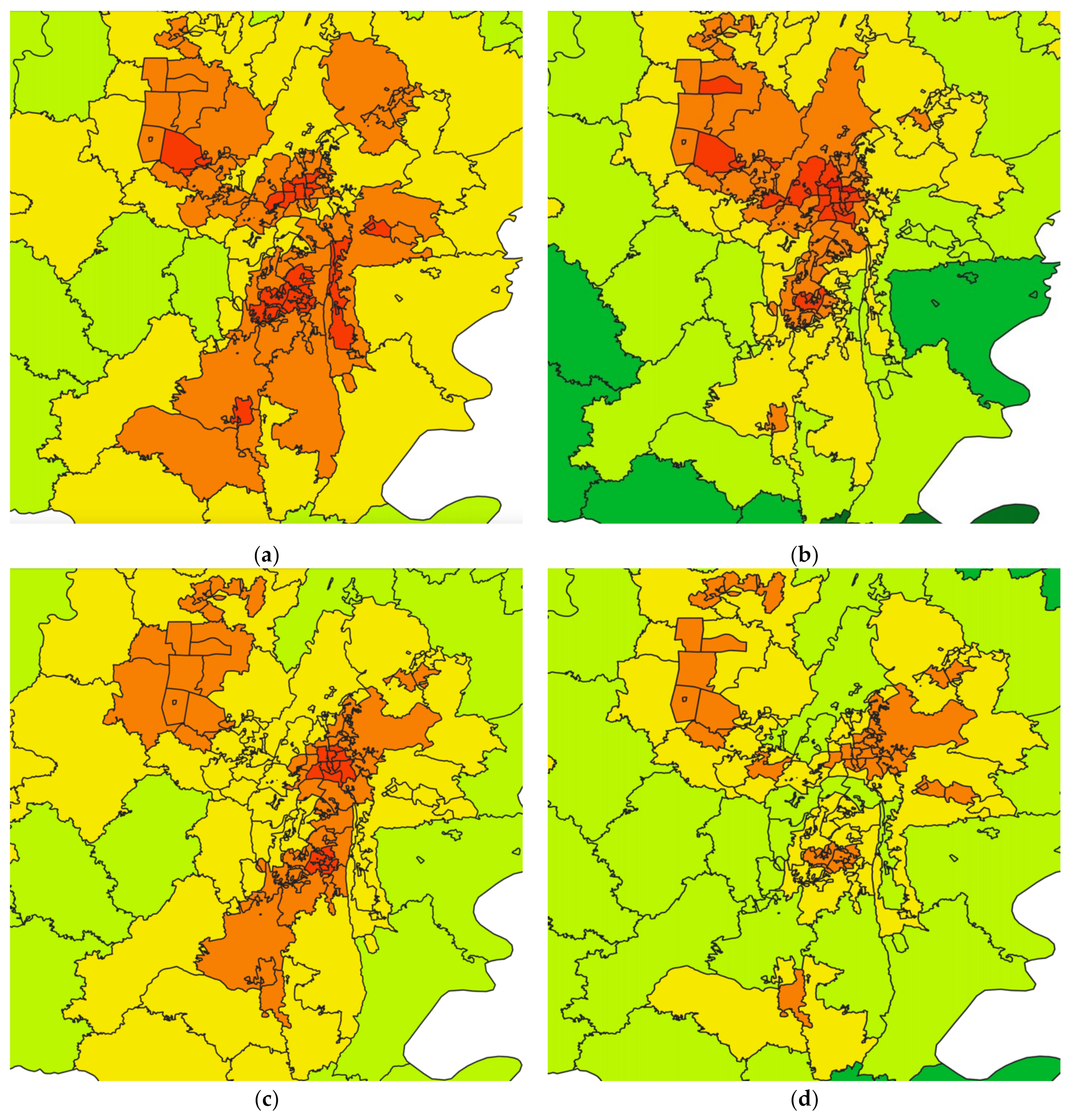
Figure 7 shows the traffic conditions at 8 o’clock, 12 o’clock, 18 o’clock and 22 o’clock on 1 October 2018 in each area of Guiyang respectively. Figure 8 shows the traffic conditions at 8 o’clock, 12 o’clock, 18 o’clock and 22 o’clock on 1 October 2018 in downtown area (within the Second Ring Road) of Guiyang respectively.

3.3. Visualization Map of Urban Hot Routes

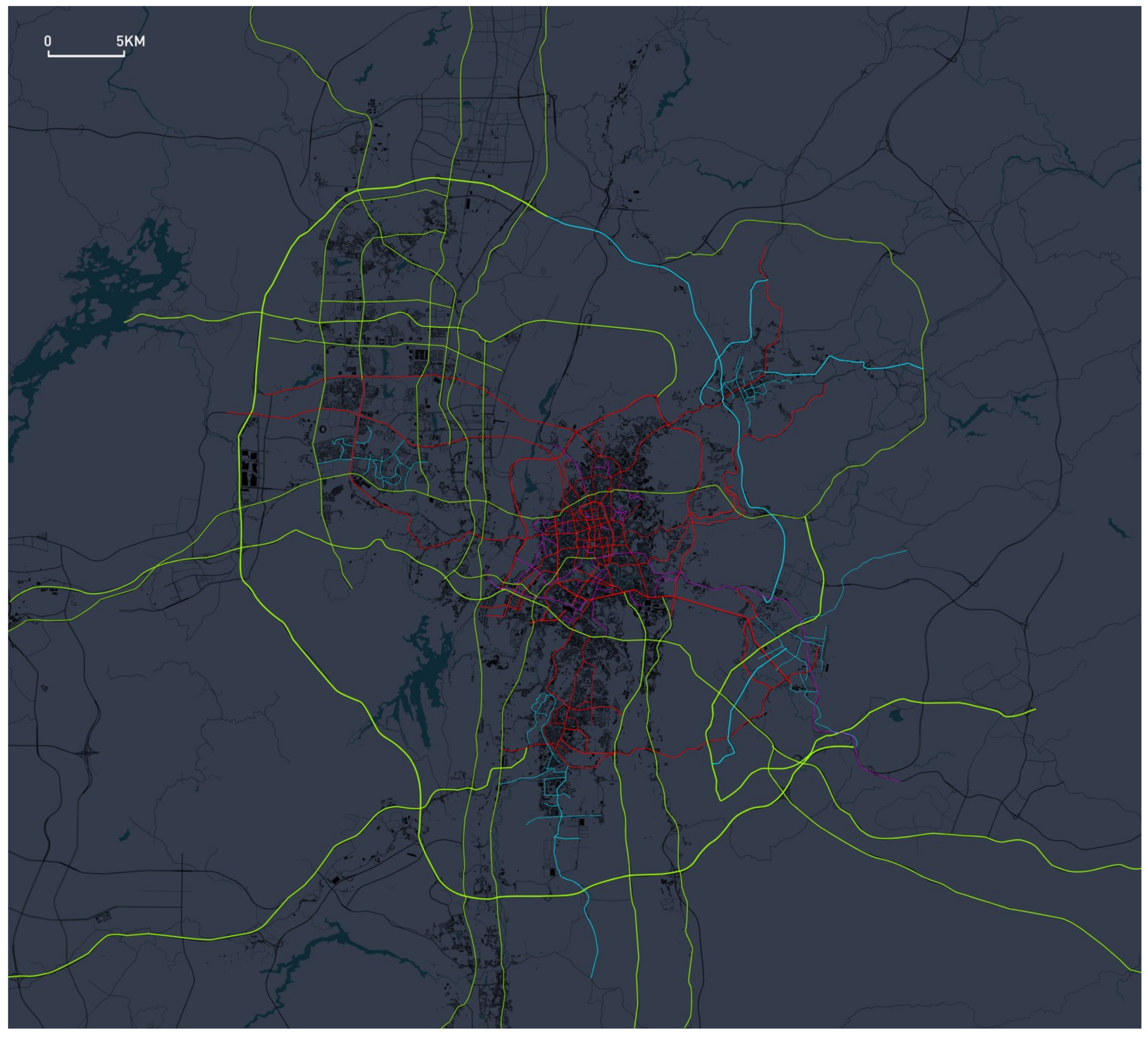
Video surveillance cameras are often located at the beginning and end of a road. Because of their unique locations, it is possible to mine hot routes. Based on the designed regional vehicle density visualization map and urban road vehicle traffic index, this paper picked 15 hot routes from areas with high traffic density. Surveillance camera data at the beginning and end of roads are screened separately. These data are then sorted according to the weight value of the number of vehicles. Determine the main traffic direction on the hot route based on the comparison of the number of vehicles at the starting point and the endpoint. The sparse distribution of surveillance cameras determines that the display of routes in the visualization map effect cannot be completed only by the connection of the surveillance camera address coordinates. This paper obtains the vector geo-information of roads from the State Geographic Information Center of China. With the help of GNU GPL license GIS software QGIS to acquire road shapes and JavaScript to design the Web-GIS page and visualization effects, a cross-platform access is finally realized. The shape of roads with high occupancy is shown in Figure 9.

Results are as shown in Figure 10, visualization map of urban hot routes reveals 15 hot lines in urban areas with high vehicle density at 8 o’clock on 1 October 2018. The main direction of traffic flow on the road is shown by moving light spots.

3.4. Mobile Devices Interface

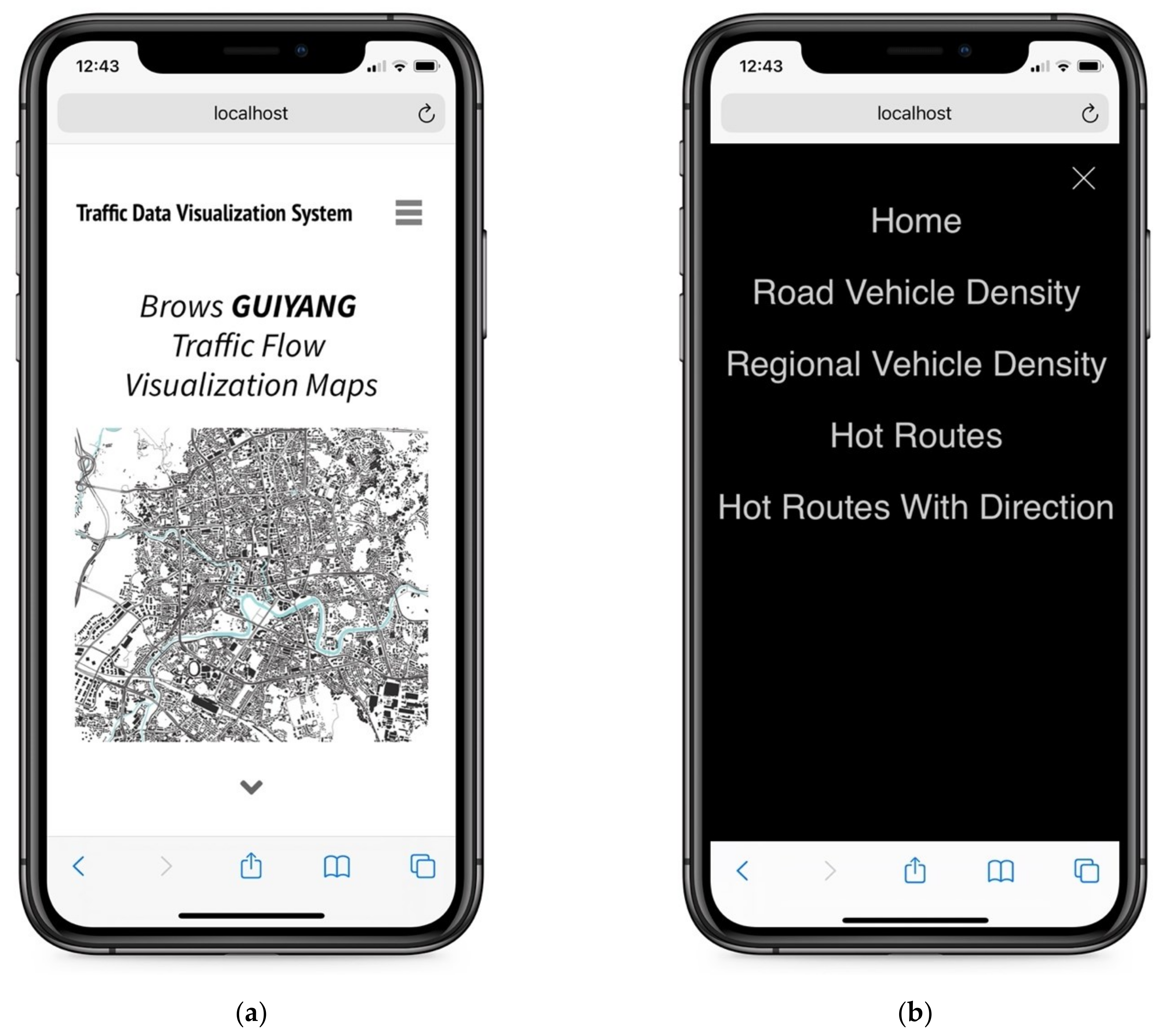
Various friendly interactive visual analytics methods are devised for exploring urban road traffic spatial and temporal characters. An interface is designed for mobile devices users to examine the analysis results as shown in Figure 11. The user can access the interface by opening the web page through a smartphone browser and select different visualization maps from the menu bar on the top.

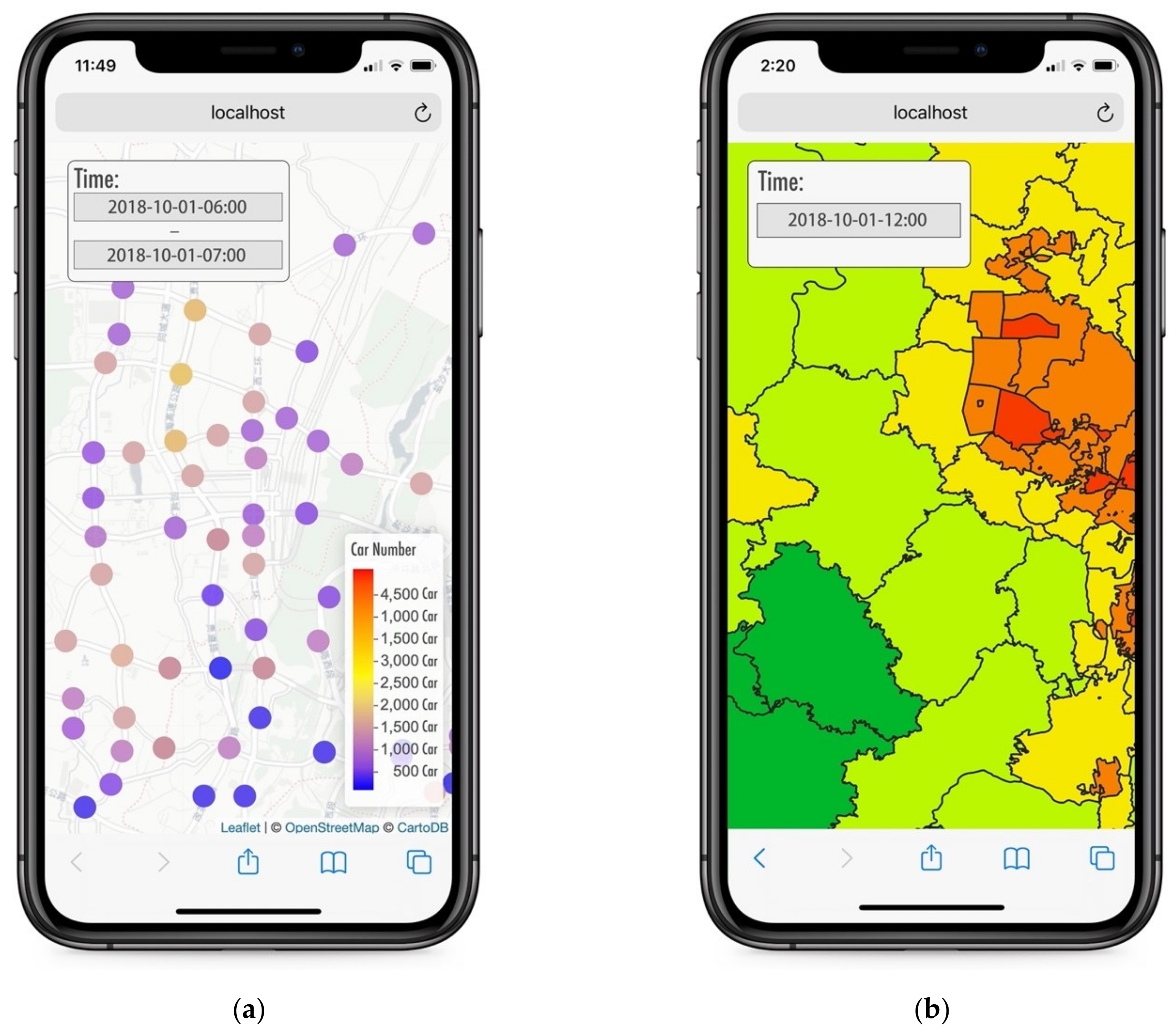
Figure 12 shows two interfaces for the road vehicle density visualization map and the regional vehicle density visualization map. User can type in a one-hour time period to check the vehicle density on urban road during that time span, the road vehicle density situation around Guiyang North Railway Station from 06:00 to 07:00 on 1 October 2018 is displayed in Figure 12a. User can also enter a specific hour time to examine the regional vehicle density information at that time, the vehicle density situation in Baiyun District at 12:00 on 1 October 2018 is displayed in Figure 12b. User can also interactively explore the analysis results of the urban hot routes visualization map as shown in Figure 13. All these map interfaces can be dragged or zoomed in and out by the user on a smartphone.

4. Discussion

The subject of this study was a spatio-temporal visualization method of urban road traffic based on video surveillance camera data. To focus on this research goal, first, we extracted the license plate data recorded by the Guiyang road video surveillance camera system, which was provided by Guiyang Transportation Department. Addresses in the license plate data are stored in text description, in order to project the address onto the map. Second, we obtained multiple groups of longitude and latitude values of address information based on Internet crawler technology. Third, we utilized the principle of statistics to design and adopt an outlier detection algorithm based on the Dixon detection method. Precise latitude and longitude information is obtained by the algorithm. Finally, based on the precise latitude and longitude of addresses information as well as the weight value of vehicles quantity, we developed three visual maps to show the spatio-temporal characteristics of vehicles on urban roads. In the design process, we established an urban road vehicle traffic index to improve the display effect of visualization map.

The current road vehicle traffic visualization methods provided by map service providers such as Google and Baidu mostly based on the data from location and quantity information of map users. Liu et al. [16] developed a traffic visual analysis method via spatio-temporal graphs, based on records of taxi global positioning system (GPS) devices. Compared with the above methods which rendering visualization map effects by user digital footprints or taxi global positioning system (GPS) devices data and display traffic trajectory information on map roads, the visualization method based on the license plate data recorded by the road surveillance camera system we designed can more directly reflect the real situation of the vehicle quantity on roads and reveal the spatial and temporal aggregation characteristics of urban regional traffic aggregation as complementary for the existing methods to understanding urban traffic characteristics.

In the process of location geo-information and map projection, the present commonly used map matching algorithm corrects the offset value of longitude and latitude according to the GPS spatio-temporal trajectory information. For the offset correction of static address longitude and latitude, we constructed an outlier detection technology based on statistics. The offset latitude and longitude values were eliminated according to the matching degree of the address geo-information and the designed model.

The spatio-temporal visualization method of urban road traffic has proven valuable. By accessing the visualization platform, citizens can clearly query and understand the traffic conditions in different areas of the city, districts, and roads. According to the visualization effects, urban residents can scientifically select travel destinations, travel times, travel modes, and travel routes, which will greatly improve travel efficiency and reduce waiting time caused by congestion. Our results suggest a possibility for urban traffic management departments to understand the general law of urban congestion and the trend of road traffic. Visualization maps can help urban road managers quickly identify traffic congestion areas, road sections and intersections, formulate and issue relevant management policies in a timely manner, and reasonably implement traffic improvement measures. Meanwhile, one important future direction of the urban road vehicle traffic index is to help urban planners systematically assess the impact of major traffic infrastructure (such as rail, trunk roads, etc.) and traffic events (special weather, traffic accidents, etc.) as the assessment objectives and quantitative evaluation means of major traffic policies.

Urban intelligent transportation system (ITS) is an effective means to improve the performance of urban traffic systems. An increasing number of traffic sensing devices are applied to it. We have tried to establish an efficient Internet of Things (IoT) platform to connect the traffic sensing devices such as urban road surveillance cameras with the visualization platform in real-time. However, this work requires multi-pronged efforts and cooperation to complete. The visualization method we designed in this paper is to read the data from the database, analyze and process the data, and finally achieve the visualization effect, there are defects in immediacy and processing speed. In the process of linearizing the point data, the method of hot spot route mining designed by us has some defects, such as consuming more resources, requiring more deo-information, relatively fixed starting and finishing points and a smaller number of routes. A future improvement in line with our research direction is to connect the visualization platform with the urban road surveillance camera systems, release the urban road traffic information in real time, and construct an efficient method for urban road hot routes mining with wide coverage and few required instances.

5. Conclusions

Understanding urban road vehicle traffic spatio-temporal characteristics benefits trip planning, traffic management and urban design. This paper proposes a visualization method for exploration of vehicle traffic spatio-temporal characteristics. Massive amounts of road video surveillance camera data are analyzed and processed to obtain geo-information. To address the problem of latitude and longitude positioning deviation, an outlier detection algorithm based on the Dixon detection method is designed for accurately projecting the geo-information to the corresponding position on the visualization map. User-friendly visualization maps are developed for the exploration of complex road traffic spatio-temporal characters in a mega-city in the spirit of visual analytics. An experiment in Guiyang was conducted using 13,094,552 pieces of data from traffic video surveillance cameras on 1 October 2018. The proposed visualization maps reveal the vehicle density on urban roads, the regional traffic conditions, and the flow of vehicles on urban hot routes. Results of the implementation and the experiment demonstrate that the presented framework provides advantageous tools for traffic analysis and future transport planning.

References

- Bui, K.H.N.; Yi, H.; Cho, J. A Multi-Class Multi-Movement Vehicle Counting Framework for Traffic Analysis in Complex Areas Using CCTV Systems. Energies 2020, 13, 2036. [Google Scholar] [CrossRef] [Green Version]
- Fernandez, S.; Hadfi, R.; Ito, T.; Marsa-Maestre, I.; Velasco, J.R. Ontology-Based Architecture for Intelligent Transportation Systems Using a Traffic Sensor Network. Sensors 2016, 16, 1287. [Google Scholar] [CrossRef]
- Sun, R.; Cheng, Q.; Xue, D.; Wang, G.; Ochieng, W. GNSS/Electronic Compass/Road Segment Information Fusion for Vehicle-to-Vehicle Collision Avoidance Application. Sensors 2017, 17, 2724. [Google Scholar] [CrossRef] [Green Version]
- Hsu, Y.W.; Chen, Y.W.; Perng, J.W. Estimation of the Number of Passengers in a Bus Using Deep Learning. Sensors 2020, 20, 2178. [Google Scholar] [CrossRef] [PubMed] [Green Version]
- Xue, Z.; Wu, W. Anomaly detection by exploiting the tracking trajectory in surveillance videos. Sci. China Inf. Sci. 2020, 63, 197–199. [Google Scholar] [CrossRef] [Green Version]
- Zhou, J.; Shen, J.; Zang, K.; Shi, X.; Du, Y.; Šilhák, P. Spatio-Temporal Visualization Method for Urban Waterlogging Warning Based on Dynamic Grading. ISPRS Int. J. Geo-Inf. 2020, 9, 471. [Google Scholar] [CrossRef]
- Fan, B.; Li, Y.; Zhang, R.; Fu, Q. Review on the Technological Development and Application of UAV Systems. Chin. J. Electron. 2020, 29, 199–207. [Google Scholar] [CrossRef]
- Wang, Q.; Lu, M.; Li, Q. Interactive, Multiscale Urban-Traffic Pattern Exploration Leveraging Massive GPS Trajectories. Sensors 2020, 20, 1084. [Google Scholar] [CrossRef] [Green Version]
- Ji, Y.; Gu, R.; Yang, Z.; Li, J.; Li, H.; Zhang, M. Artificial intelligence-driven autonomous optical networks: 3S architecture and key technologies. Sci. China Inf. Sci. 2020, 63, 7–30. [Google Scholar] [CrossRef]
- Villalpando, F.; Tuxpan, J.; Ramos-Leal, J.A.; Carranco-Lozada, S. New Framework Based on Fusion Information from Multiple Landslide Data Sources and 3D Visualization. J. Earth Sci. 2019, 31, 159–168. [Google Scholar] [CrossRef]
- Wu, S.; Tao, L. Building Height Trends and Their Influencing Factors under China’s Rapid Urbanization: A Case Study of Guangzhou, 1960–2017. Chin. Geogr. Sci. 2020, 30, 993–1004. [Google Scholar]
- Yang, J. Big data and the future of urban ecology: From the concept to results. Sci. China Earth Sci. 2020, 63, 1443–1456. [Google Scholar] [CrossRef]
- Niu, F.; Yang, X.; Zhang, X. Application of an evaluation method of resource and environment carrying capacity in the adjustment of industrial structure in Tibet. J. Geogr. Sci. 2020, 30, 319–332. [Google Scholar] [CrossRef]
- Triboan, D.; Chen, L.; Chen, F.; Wang, Z. Towards a Service-Oriented Architecture for a Mobile Assistive System with Real-time Environmental Sensing. Tsinghua Sci. Technol. 2016, 21, 581–597. [Google Scholar] [CrossRef]
- Altintasi, O.; Tuydes-Yaman, H.; Tuncay, K. Detection of urban traffic patterns from Floating Car Data (FCD). Transp. Res. Procedia 2017, 22, 382–391. [Google Scholar] [CrossRef]
- Liu, L.; Zhan, H.; Liu, J.; Man, J. Visual analysis of traffic data via spatio-temporal graphs and interactive topic modeling. J. Vis. 2018, 22, 141–160. [Google Scholar] [CrossRef]
- Zhang, X.; Zhang, Q.; Lv, M.; Li, S. Mining urban hot routes based on spatio-temporal license plate number data. Chin. High Technol. Lett. 2020, 30, 676–686. [Google Scholar]
- Andrienko, G.; Andrienko, N.; Bak, P.; Keim, D.; Wrobel, S. Visual Analytics of Movement; Springer Publishing Company: New York, NY, USA, 2013; pp. 1252–1263. [Google Scholar]
- Quek, C.; Pasquier, M.; Lim, B.B.S. POP-TRAFFIC: A novel fuzzy neural approach to road traffic analysis and prediction. IEEE Trans. Intell. Transp. Syst. 2006, 7, 133–146. [Google Scholar] [CrossRef]
- Pritchard, R.; Frøyen, Y.; Snizek, B. Bicycle Level of Service for Route Choice—A GIS Evaluation of Four Existing Indicators with Empirical Data. ISPRS Int. J. Geo-Inf. 2019, 8, 214. [Google Scholar] [CrossRef] [Green Version]
- Mo, B.; Li, R.; Zhan, X. Speed profile estimation using license plate recognition data. Transp. Res. Part C Emerg. Technol. 2017, 82, 358–378. [Google Scholar] [CrossRef]
- Liu, Z.; Li, R.; Wang, X. Effects of vehicle restriction policies: Analysis using license plate recognition data in Langfang, China. Transp. Res. Part A Policy Pract. 2018, 118, 89–103. [Google Scholar] [CrossRef]
- Zhan, X.; Li, R.; Ukkusuri, S.V. Lane-based real-time queue length estimation using license plate recognition data. Transp. Res. Part C Emerg. Technol. 2015, 57, 85–102. [Google Scholar] [CrossRef]
- Khan, P.; Byun, Y.-C.; Park, N. A Data Verification System for CCTV Surveillance Cameras Using Blockchain Technology in Smart Cities. Electronics 2020, 9, 484. [Google Scholar] [CrossRef] [Green Version]
- Mandal, V.; Mussah, A.R.; Jin, P.; Adu-Gyamfi, Y. Artificial Intelligence-Enabled Traffic Monitoring System. Sustainability 2020, 12, 9177. [Google Scholar] [CrossRef]
- Lin, C.B.; Hung, R.W.; Hsu, C.Y.; Chen, J.S. A GNSS-Based Crowd-Sensing Strategy for Specific Geographical Areas. Sensors 2020, 20, 4171. [Google Scholar] [CrossRef] [PubMed]
- Dahl, M.; Javadi, S. Analytical Modeling for a Video-Based Vehicle Speed Measurement Framework. Sensors 2019, 20, 160. [Google Scholar] [CrossRef] [PubMed] [Green Version]
- Beyer, K.S.; Ercegovac, V.; Gemulla, R. Jaql: A scripting language for large scale semi structured data analysis. Proc. VLDB Endow. 2011, 4, 1272–1283. [Google Scholar] [CrossRef]
- Harmon, L.J.; Weir, J.T.; Brock, C.D. GEIGER: Investigating evolutionary radiations. Bioinformatics 2008, 24, 129–131. [Google Scholar] [CrossRef] [Green Version]
- Demant, J.; Munksgaard, R.; Houborg, E. Personal use, social supply or redistribution? Cryptomarket demand on Silk Road 2 and Agora. Trends Organ. Crime 2018, 21, 42–61. [Google Scholar] [CrossRef]
- Okoampa-Larbi, R.; Twum, F.; Hayfron-Acquah, J.B. A Proposed Cloud Security Framework for Service Providers in Ghana. Int. J. Comput. Appl. 2017, 975, 8887. [Google Scholar] [CrossRef]
- Patel, R.; Bhatt, P. A Survey on Semantic Focused Web Crawler for Information Discovery Using Data Mining Technique. Int. J. Innov. Res. Sci. Technol. 2014, 1, 168–170. [Google Scholar]
- Boukadi, K.; Rekik, M.; Rekik, M.; Ben-Abdallah, H. FC4CD: A new SOA-based Focused Crawler for Cloud service Discovery. Computing 2018, 100, 1081–1107. [Google Scholar] [CrossRef]
- Ohana-Levi, N.; Knipper, K.; Kustas, W.P.; Anderson, M.C.; Netzer, Y.; Gao, F.; Alsina, M.D.M.; Sanchez, L.A.; Karnieli, A. Using Satellite Thermal-Based Evapotranspiration Time Series for Defining Management Zones and Spatial Association to Local Attributes in a Vineyard. Remote Sens. 2020, 12, 2436. [Google Scholar] [CrossRef]
- Takenaka, H.; Sakashita, T.; Higuchi, A.; Nakajima, T. Geolocation Correction for Geostationary Satellite Observations by a Phase-Only Correlation Method Using a Visible Channel. Remote Sens. 2020, 12, 2472. [Google Scholar] [CrossRef]
- Zhao, G.; Chen, A.; Lu, G.; Liu, W. Data Fusion Algorithm Based on Fuzzy Sets and D-S Theory of Evidence. Tsinghua Sci. Technol. 2020, 25, 12–19. [Google Scholar] [CrossRef]
- Zhao, X.; Cheng, X.; Zhou, J. Advanced topological map matching algorithm based on D–S theory. Arab. J. Sci. Eng. 2018, 43, 3863–3874. [Google Scholar] [CrossRef]
- Hashemi, M.; Karimi, H.A. A critical review of real-time map-matching algorithms: Current issues and future directions. Comput. Environ. Urban Syst. 2014, 48, 153–165. [Google Scholar] [CrossRef]
- Kavzoglu, T.; Tonbul, H. An experimental comparison of multi-resolution segmentation, SLIC and K-means clustering for object-based classification of VHR imagery. Int. J. Remote Sens. 2018, 39, 6020–6036. [Google Scholar] [CrossRef]
- Teng, W.; Wang, Y. Real-time map matching: A new algorithm integrating spatio-temporal proximity and improved weighted circle. Open Geosci. 2019, 11, 288–297. [Google Scholar] [CrossRef]
- Campello, R.J.G.B.; Moulavi, D.; Zimek, A. Hierarchical density estimates for data clustering, visualization, and outlier detection. ACM Trans. Knowl. Discov. Data 2015, 10, 1–51. [Google Scholar] [CrossRef]
- Kodinariya, T.M.; Makwana, P.R. Review on determining number of Cluster in K-Means Clustering. Int. J. 2013, 1, 90–95. [Google Scholar]
- Cohn, T.A.; England, J.F.; Berenbrock, C.E. A generalized Grubbs-Beck test statistic for detecting multiple potentially influential low outliers in flood series. Water Resour. Res. 2013, 49, 5047–5058. [Google Scholar] [CrossRef]
- Gupta, M.; Gao, J.; Aggarwal, C.C. Outlier detection for temporal data: A survey. IEEE Trans. Knowl. Data Eng. 2013, 26, 2250–2267. [Google Scholar] [CrossRef]
- Gupta, M.; Gao, J.; Aggarwal, C. Outlier detection for temporal data. Synth. Lect. Data Min Knowl. Discov. 2014, 5, 1–129. [Google Scholar] [CrossRef]
- Hongquan, S. Real-time monitoring for crowd counting using video surveillance and GIS. In Proceedings of the 2012 IEEE 2nd International Conference on Remote Sensing, Environment and Transportation Engineering, Nanjing, China, 1–3 June 2012; pp. 1–4. [Google Scholar]
- Demissie, M.G.; de Almeida Correia, G.H.; Bento, C. Intelligent road traffic status detection system through cellular networks handover information: An exploratory study. Transp. Res. Part C Emerg. Technol. 2013, 32, 76–88. [Google Scholar] [CrossRef]
- Yu, R.; Wang, G.; Zheng, J. Urban road traffic condition pattern recognition based on support vector machine. J. Transp. Syst. Eng. Inf. Technol. 2013, 13, 130–136. [Google Scholar] [CrossRef]
- Jia, S.; Peng, H.; Liu, S. Urban traffic state estimation considering resident travel characteristics and road network capacity. J. Transp. Syst. Eng. Inf. Technol. 2011, 11, 81–85. [Google Scholar] [CrossRef]
- Dong, Y.; Xu, J.; Liu, X.; Gao, C.; Ru, H.; Duan, Z. Carbon emissions and expressway traffic flow patterns in China. Sustainability 2019, 11, 2824. [Google Scholar] [CrossRef] [Green Version]
- Jiang, S.; Babovic, V.; Zheng, Y.; Xiong, J. Advancing opportunistic sensing in hydrology: A novel approach to measuring rainfall with ordinary surveillance cameras. Water Resour. Res. 2019, 55, 3004–3027. [Google Scholar] [CrossRef]
- Zhang, L.; Hu, X.; Qiu, R.; Lin, J. Comparison of real-world emissions of LDGVs of different vehicle emission standards on both mountainous and level roads in China. Transp. Res. Part D Transp. Environ. 2019, 69, 24–39. [Google Scholar] [CrossRef]
- Luo, J.; Du, P.; Samat, A.; Xia, J.; Che, M.; Xue, Z. Spatiotemporal pattern of PM 2.5 concentrations in mainland China and analysis of its influencing factors using geographically weighted regression. Sci. Rep. 2017, 7, 1–14. [Google Scholar]
- Chen, B.; Ye, Z.N.; Chen, Z.; Xie, X. Bridge vehicle load model on different grades of roads in China based on Weigh-in-Motion (WIM) data. Measurement 2018, 122, 670–678. [Google Scholar] [CrossRef]
Figure 1.
Visualization map of comparison between the longitude and latitude data determined by the algorithm and provided by the government. (a) Checkpoint of Guiyang North Toll Station Bayonet. (b) Checkpoint of Zazuo Toll Station of Guiyang-Bixi Expressway. (c) Entrance of Daguan Tunnel on Qianlingshan Road. (d) Checkpoint of Shibanshao Toll Station Bayonet. (e) Checkpoint of Mengguan Toll Station Bayonet. (f) Yuan Tunnel Entrance of Beijing East Road. (g) Checkpoint of Shangmai Toll Station Bayonet. (h) Guiyang East Exit Expressway Toll Station. (i) Entrance of Xiaoguan Tunnel on Central Ring North Line. (j) Military Area South Factory Road Longmen Viaduct.