
Crime against Businesses: Temporal Stability of Hot Spots in Mexicali, Mexico


Instituto de Investigaciones Sociales, Universidad Autónoma de Baja California, Edificio de Investigación Posgrado, Unidad Universitaria, Mexicali C. P. 21280, Baja California, Mexico
*
Author to whom correspondence should be addressed.
ISPRS Int. J. Geo-Inf. 2021, 10(3), 178; https://0-doi-org.brum.beds.ac.uk/10.3390/ijgi10030178
Submission received: 11 February 2021
/
Revised: 2 March 2021
/
Accepted: 15 March 2021
/
Published: 17 March 2021
Abstract
:In developing countries, crime is a serious problem that affects the operation and viability of firms. Offenses such as vandalism, robbery, and theft raise the operating costs of firms and imposes on them indirect costs. The literature on spatial analysis of crime is vast; however, relatively little research has addressed business crime, especially in developing countries’ cities. Spatial and temporal analysis of crime concentration represents a basic input for the design and implementation of appropriate prevention and control strategies. This article explores the spatial concentration and stability of thefts committed against commercial establishments in the city of Mexicali, Mexico, from 2009 to 2011 using the Gini coefficient, Lorenz curve, and decile maps. Results revealed that thefts were highly concentrated in a small percentage of urban basic geostatistical areas. Moreover, a portion of these areas were classified as having the highest deciles of thefts (hot spots) and remained in this group throughout the period. In both cases, the relationship between crime and place was close to the 80/20 rule, or the Pareto principle.
1. Introduction
Firms make a significant contribution to the economic and social development of cities and countries (jobs, tax revenues, income, investments). Hence, any threat to their survival or growth eventually affects the welfare of the local community. Due to their characteristics and location, some businesses may be exposed to higher crime rates than others, and be more vulnerable to this hazard.
In developing countries, crime has become a major problem that threatens the operation and viability of businesses. Crime represents different direct costs, such as lost earnings, property damage, private security expenditures, and increase of insurance premiums. Crime also imposes indirect costs on businesses, such as loss of customers due to a perceived lack of security, fearful employees because of repeated victimization, among others [1,2,3].
In 2014 in Latin America and the Caribbean, crime costs represented 3.5% of the gross domestic product, and twice the average cost in developed countries [4]. For this reason, 35% of firms in Latin America identified crime as one of the main problems in maintaining their business activities [5].
Spelman [6]; Johnson [7]; and Weisburd, Bushway, Lum, and Yang [8] indicate that spatial and temporal analysis of crime concentration is a basic tool in the design and implementation of appropriate prevention and control strategies [6,7,8]. That is, if crime concentrates and remains stable in certain places over time, crime reduction strategies could be more efficient and effective if resources and activities are focused on them [9]. However, most studies addressing these topics focus on crime in developed countries’ cities, while relatively little have been published on developing countries, especially on crime against business [10,11].
In Mexico, the levels of crime and violence have severely affected the business sector to such a degree that, after corruption and inefficient government bureaucracy, crime and theft have been considered among the most problematic factors for businesses [12]. The results of the 2012 National Survey on Business Victimization revealed that theft or assault accounted for 22.6% of all crimes against businesses in the country. They also indicated that the commerce sector was more affected by crime than other economic sectors (industry, 12%; services, 38.3%; and commerce, 49.7%) [13].
Baja California ranks among the states with the highest rates of crime against businesses in the country (with 4504 crimes per 10,000 establishments) [13]. Tijuana and Mexicali are the largest municipalities in this state (49.4% and 29.7% of the population, respectively) [14]. From 2010 to 2011, Mexicali moved from second to first place in thefts committed against businesses in the state, and its total thefts increased by 76% [15]. This happened despite the fact that commercial establishments only increased by 18.5% from 2008 to 2013 in this municipality [16,17].
The changes in the number of thefts in a short period and their spatial distribution are issues of interest in our research, giving rise to the next questions: (1) Does the concentration ratio of thefts against businesses approach the 80/20 rule in Mexicali from 2009 to 2011? (2) Do hot spots remain stable during the period? Therefore, the general objective of this article is to explore the spatial and temporal stability of hot spots of thefts against commercial establishments in the city of Mexicali from 2009 to 2011 using crime data by basic geostatistical area.
2. Crime Concentration
Brantingham and Brantingham [18] (p. 79) state, “Crimes do not occur randomly or uniformly in time or space or society […] There are hot spots and cold spots; there are high repeat offenders and high repeat victims.” Routine flow of people and goods depends on the location of facilities, which influences the pattern of crime concentration. Each urban environment has a spatial array that integrates at least a street network and a set of land uses organized along it. Suitable crime targets, such as residences or businesses, have a fixed location, and they tend to agglomerate in certain zones of the city, influencing crime spatial distribution [18,19]. The term “hot spot” is commonly used to refer to a crime concentration area and includes spatial units, such as addresses, blocks, and neighborhoods [20,21,22,23].
More precisely, “hot spot” is defined as “an area that has a greater than average number of criminal or disorder events, or an area where people have a higher than average risk of victimization” [24] (p. 2). However, the identification of hot spots through an average of crimes shows disadvantages when the range of offenses between areas is very high. Consequently, to avoid this problem and simplify the analysis of crime concentration, we understand hot spots as areas that occupy the highest deciles in the distribution of crime in the city in a particular period.
Several studies examine hot spots for different sizes of cities, types and numbers of crimes, periods, and units of analysis [6,8,10,20,25,26,27,28,29,30]. They have common elements that can be grouped into the following statements: (1) crime concentration ratio is constant over time (ratio stability), and (2) crime concentration areas remain stable through time (hot spot stability).
2.1. Crime Concentration Ratio Stability: 80/20 Rule
In recent decades, growing empirical evidence supports the theory that a small proportion of facilities or specific locations suffer for most of the offenses. Eck, Clarke, and Guerette [21] propose the term “risky facilities” to explain crime concentration in a small group of facilities, finding evidence for different types of establishments. For example, in Danvers, Massachusetts, they found that 84.9% of shoplifting incidents were committed in 20.3% of the stores; in Shawnee, Kansas, 20% of the bars accounted for 62% of calls to the police; and 30% of the taverns experienced about 80% of violent incidents in Milwaukee, Wisconsin [25]. The regularity found in the distribution of crime across different facilities was named by Wilcox and Eck [31] the “iron law of troublesome places,” indicating that few places or locations have most of the trouble.
Andresen and Malleson [32] analyzed crime concentration for different offenses and spatial units (census tract, dissemination area or census block, and street segments). They found that 50% of offenses were committed in the range of 1% to 8% of street segments according to the category of crime. Moreover, ratios of certain offenses tended to remain relatively stable over time. This result is similar to what Levin, Rosenfeld, and Deckard [33]; Steenbeek and Weisburd [34]; and Andresen and Linning [35] reported.
Weisburd [36] proposed a ‘‘law of crime concentration” as a result of a literature review on crime concentration in developed countries’ cities. The author found that 50% of offenses occurred within 2% to 6% of the street segments, and observed that although the number of crimes changed widely over time, concentration levels remained stable with a ratio of 50/5; that is, 50% of offenses were committed in 5% of street segments.
Fuentes and Hernández [37] examined the concentration of violent crimes in Ciudad Juarez, Mexico, using basic geostatistical areas and census blocks as analysis units. They obtained a concentration ratio of 79/33 at the geostatistical area level and a relationship of approximately 65/18 at the block level. Melo, Matias, and Andresen [38] examined different types of offenses in Campinas, Brazil. Overall, they found a concentration ratio of all criminal events of 50/10 at the census tract level and 50/4 at the segment street level.
Jaitman and Ajzenman [10] examined four cities in developing countries—Montevideo, Uruguay; Bogota, Colombia; Belo Horizonte, Brazil; and Zapopan, Mexico—and performed a partial analysis for Sucre, Venezuela, and found that 50% of crimes were concentrated in the range of 3% to 7.5% of street segments. Their results were consistent with research on developed countries’ cities.
Regularities in the distribution of criminal events across places are commonly known as the 80/20 rule or the Pareto principle. This rule states, “In theory 20 percent of any particular group of things is responsible for 80 percent of outcomes” [25] (p. 4). Although this relationship is seldom exactly 80/20, it is useful as an initial hypothesis and more appropriate than assuming that the distribution of crime occurs uniformly in the city.
2.2. Temporal Stability of Hot Spots
Empirical evidence shows that a few places or facilities concentrate large amount of crimes. They are called hot spots and indicate a concentration of crime opportunities that result from the convergence in space and time of suitable targets and motivated offenders without capable guardians. Therefore, rational choices are situationally specific (materialized in a particular time and space) [39,40,41,42].
Furthermore, there is a high possibility that crime concentration areas or hot spots can persist as such for a certain period. Schuerman and Kobrin [43] examined census tract clusters with the highest crime rates over 2 decades. According to the authors, there are three stages of development:
(1) Emerging: relatively new crime areas that were virtually crime free at the beginning of the period, but decades later reached a high level; (2) transitional: areas that initially showed moderately high criminal activity, which increased in the following decades; and (3) enduring: areas with crime-high densities during the entire 2 decades of study, which represents persistence of hot spots.
Cohen and Tita [44] analyzed homicide movements from one neighborhood to another, using the term “contagious diffusion,” instead of spatial adjacency, to report two spatial dynamics: relocation and expansion. They found that expansion diffusion between neighboring census tracts occurred only in the year with more crimes, while for the rest of the years, the increase of crimes happened simultaneously in non-neighboring census tracts (diffusion by relocation). However, they also observed that a census tract, including hot spots, could experience a significantly decreasing homicide rate after having a high increasing rate, as evidence of the spatial instability of crime over time.
According to Weisburd et al. [45], places that concentrate crime could suffer a process of cooling down, while the ones that are cool can become hot and replace them (heat up); therefore, crime concentration is generally moving from one location to another. On this subject, Hibdon, Telep, and Groff [46]; Andresen, Linning, and Malleson [47]; and Levin, Rosenfeld, and Deckard [33] found that places that rank at the top of the distribution of crime vary over time, which implies an unstable spatial pattern of hot spots.
The application of measures of prevention and control can modify the spatial pattern of crime. These actions could discourage criminal incidence where they are applied and transfer it to other areas [26]. In this regard, Guerette [48] states that, if the intervened area is a crime attractor, it is highly probable that crime displacement occurs towards adjacent areas (expansion diffusion).
Nevertheless, as indicated by Weisburd and Telep [49], this spatial displacement will take effect only if these areas share the same characteristics of places where crime has been reduced. Otherwise, these measures can lead to crime decrease around the intervened zone as a result of spatial diffusion of security [48], and crime transfer to more distant areas (diffusion by relocation).
The characteristics of the urban environment that structure the spaces of human activities in the city influence opportunities to commit crimes.
The urban settings that create crime and fear are human constructions, the by-product of the environments we build to support the requirements of everyday life: homes and residential neighborhoods; shops and offices; factories and warehouses; government buildings; parks and recreational sites; sports stadia and theaters; and transport systems, bus stops, roadways, and parking garages. The ways in which we assemble these large building blocks of routine activity into the urban backcloth can have an enormous impact on our fear levels and the quantities, types, and timing of the crimes we suffer [50] (p. 5).
In this sense, commercial activities have been categorized as attractors and generators of crimes, because they combine characteristics that offer known opportunities to commit offenses and are frequented by large numbers of people [51].
Nonetheless, Weisburd [36] (p. 148) asks, “Does crime concentration reflect concentrated activity in the other areas of social life? If so, then it suggests that we need to broaden our lens and recognize that crime is only one of a series of phenomena that are concentrated in the modern city.” Consequently, the stability of hot spots can be the result of the normal concentrations of other social and economic activities in the city.
3. Materials and Method
3.1. Area of Study
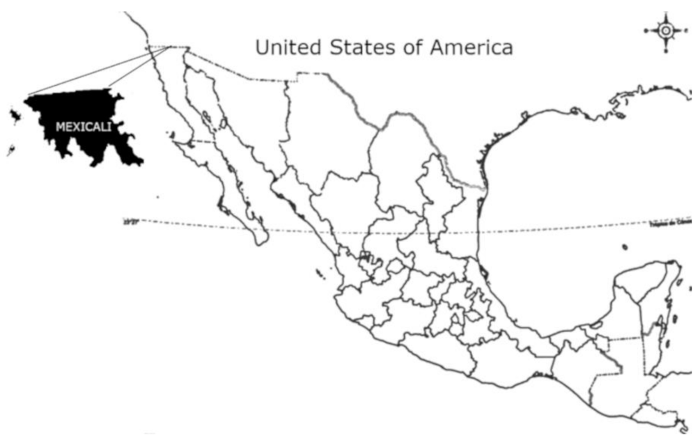
Mexicali is a border city located in the northwest of Mexico in the state of Baja California (Figure 1). The origin and urban expansion of Mexicali were initially related to the investment in the agricultural sector and later to the industrial policy that promoted the installation of maquiladoras. Maquiladora plants emerged with the Mexican Border Industrialization Program introduced in 1965. The industrialization process stimulated rapid increase in urban population [52,53], as well as the growth and diversification of commerce, services, and supporting industries in the city [54].
According to the results of the 2009 Economic Census [16], in Mexicali, approximately 37 out of every 100 establishments were dedicated to commercial activities—4% wholesale and 33% retail. Employees in this sector were concentrated in retail (78%), and most retail businesses were grocery and convenience stores.
The distribution of commercial establishments in the city is uneven (Figure 2). The areas with the highest number of firms are located near the main roads and the central area of the city. The density of businesses tends to decrease towards the periphery and secondary roads. Since commercial establishments are theft-suitable targets, the urban pattern of firms may be similar to the spatial distribution of crime. However, crime concentration is dynamic; it changes in space over time, generating new spatial patterns.
3.2. Data
The spatial unit of analysis in this research is the Basic Geostatistical Area (AGEB for its acronym in Spanish). In Mexico, the National Institute of Statistics and Geography (INEGI) divides cities into AGEBs for census purposes. An AGEB is a relatively homogeneous urban area that groups blocks perfectly defined by streets, avenues, sidewalks or any other easily identifiable characteristics in the space and the land use [55]. In 2010, INEGI divided the city of Mexicali into 381 AGEBs (average of 45.61 hectares).
We used official records of thefts in commercial establishments that occurred in Mexicali from 2009 to 2011 provided by the Procuraduría General de Justicia del Estado de Baja California (PGJEBC for its acronym in Spanish) [15]. The database registers the colony where the thefts occurred; therefore, thefts were geocoded at this spatial unit and, subsequently, assigned to the AGEB level using a weighted allocation process.
The temporal frame includes the year with the highest theft incidence in Mexicali (2011), which was when the municipality ranked first in this offense in the state of Baja California. It also includes the years in which INEGI carried out the censuses, in order to relate crime frequency to economic and sociodemographic data. Sociodemographic data were retrieved from the 2010 Population and Housing Census [14]; basic economic data for commercial establishments were obtained from the 2009 Economic Census [16] and National Directory of Economic Units [56]. All variables were included as layers in a geographic information system and processed at the AGEB level.
3.3. Measuring Concentration and Stability
In accordance with the literature suggesting that crime is a spatial phenomenon, which concentrates in a few places and remains stable in space and time, the central questions in this study are the following: (1) Does the concentration ratio of thefts against businesses approach the 80/20 rule in Mexicali from 2009 to 2011? (2) Do hot spots remain stable during the period? Applying the 80/20 rule means that each year, 80% of thefts occurred in 20% of all AGEBs, and stability of hot spots occurs when more than half of them remain stable within the 3 years.
To answer the first question, we used three statistical tools: decile maps, Lorenz curve, and Gini index. Decile maps allowed the arranging and grouping of AGEBs into 10 equal parts with respect to the values obtained for three crime variables: total number of thefts (R1), rate of thefts per establishment (R2), and density of thefts per hectare (R3). Deciles I and II correspond to 20% of the AGEBs with the lowest values for each variable, while deciles IX and X correspond to 20% of the AGEBs with the highest values. For the city of Mexicali, each decile has approximately 38 AGEBs.
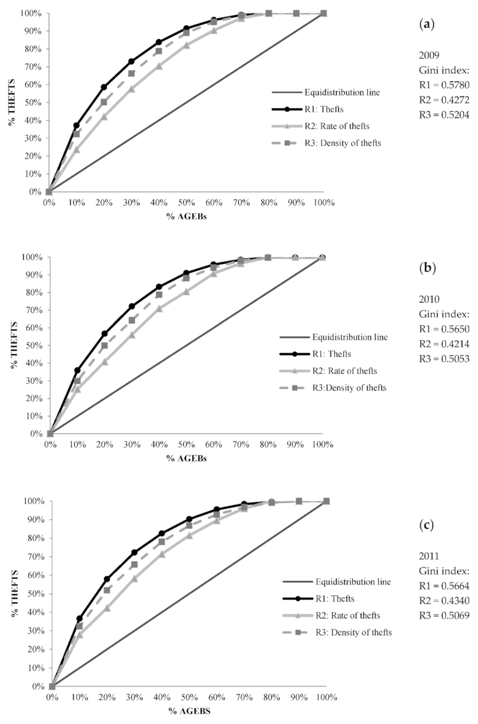
The Lorenz curve (LC) has been applied to crime concentration analysis [57,58]. LC is a graphical representation of the frequency distribution of the variable of interest with regard to the selected spatial units. In this study, the LC displays the accumulated percentages of theft (y-axis) and the accumulated percentage of AGEBs in which these crimes occurred (x-axis). The curve obtained is compared with the equidistribution line (EL) that represents a hypothetical perfect distribution of crime among the AGEBs (45-degree line). If all crimes were equally distributed among all the spatial units, the LC coincides with the EL, while a greater separation of the lines indicates a higher concentration level of crime [57].
The Gini index (G) is based on the Lorenz Curve and assumes values from 0 to 1, in such a way that when G is equal to zero, it means that both curves (LC and EL) coincide and that offenses are distributed uniformly among the spatial units; and when G is equal to 1, crimes concentrate in only one spatial unit. The equation is as follows [57].
In this case, n is the total number of deciles, yi is the ratio of crimes that took place on each decile, and i is the position (rank) that the deciles occupy when they are ordered.
In order to answer the second question, we first selected the variable (R1, R2, or R3) with the closest ratio to the 80/20 rule. Then, we classified as hot spots the group of AGEBs belonging to the deciles with the highest number of crimes at the beginning of the period (2009). Subsequently, we identified the AGEBs that remained in the group with the highest deciles throughout the period as stable or enduring hot spots; those that remained in such a group for only 1 or 2 years were unstable or transitional hot spots. Depending on whether the AGEBs left or entered a group, they were classified as transitional 1 (dissipating hot spot) or transitional 2 (emerging hot spot), respectively. Finally, we calculated the percentage of stable or enduring hot spots to verify crime spatial stability (whether more than 50% of the AGEBs remained hot spots during the period).
4. Results
4.1. Stable Levels of Concentration: 80/20 Rule
In the city of Mexicali, in 2009 to 2011, there were 6836 thefts (R1), the rate of thefts per establishment was 0.93 (R2), and 0.40 theft was committed per hectare (R3). Theft against businesses showed an upward trend. From 2009 to 2010, there was a 21% increase in the number of reported thefts, followed by a 69% increase from 2010 to 2011.
The decile table allows us to observe the concentration levels for each variable (Table 1). For R1, 20% of the AGEBs (deciles IX and X) were grouped between 57% and 59% of total thefts in the city, lower than the 80/20 ratio expected. Nevertheless, with the addition of decile VIII (30% of the AGEBs), crime percentage ranged between 72% and 73% (70/30 ratio), closer to the 80/20 rule.
For the theft rate per establishment (R2), 20% of the AGEBs accounted for only 41% to 42% of all offenses, which means a greater spatial dispersion of R2 with respect to R1, and R2 is farther away from the 80/20 rule than R1, even if decile VIII is added. Meanwhile, for density of thefts per hectare (R3), 20% of the AGEBs comprised between 50% and 52% of all offenses, and if decile VIII is included, the range gets between 64/30 and 66/30 (Table 1). Therefore, R3 is closer than R2 to the 80/20 rule, but it is farther than R1.
The differences in the concentration ratios of the variables (R1, R2, and R3) emphasize the need to consider some aspects in their selection and use in the case of Mexicali. In particular, for R2, deciles VIII, IX, and X (top group) included AGEBs that had few crimes and few firms, contributing very little to the total of thefts in the city. This may be related to the predominance of residential, industrial, recreational, and public services land uses, regarding the commercial one. Conversely, some AGEBs were classified in lower deciles because they had numerous businesses and many crimes, which results in a low rate. This occurred mainly in commercial land use zones.
In the case of R3, some AGEBs in the 70/30 group coincide with those obtained for R1, with the exception of two small subgroups. The first subgroup includes AGEBs classified in the top group because they had a small surface area with intermediate amounts of thefts. The second subgroup includes AGEBs classified in lower deciles because they had numerous thefts and a large surface area. This subgroup includes AGEBs with a significant percentage of vacant land surface; most of them were located in the urban periphery, as industrial parks, enclosed neighborhoods, or private residential areas. The above points emphasize the influence of some aspects in the exclusion or integration of AGEBs within a 70/30 group, specifically the disadvantages presented in using R2 and R3.
4.2. Lorenz Curve and Gini Index
Lorenz curves (LCs), equidistribution lines (ELs), and Gini indexes (Gs) are shown in Figure 3. The three graphs reveal, as expected, that few places concentrated a high number of crimes in the studied period. The Gini index shows similarities during the period for each variable. This could be explained by the stability in the concentration of crimes in a few places, despite the increase in the number of crimes in the city. These results indicate that the Gini index was not overly sensitive to changes in quantities of theft during the period.
4.3. Temporal Stability of Hot Spots
Based on the above results and considering the disadvantages of the use of the theft rate and theft density (R2 and R3), we selected the number of thefts (R1) to examine the spatial stability pattern of hot spots.
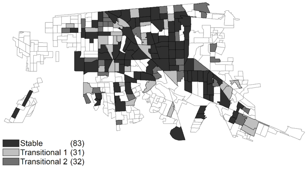
The next step of the analysis was to verify whether more than 50% of the hot spots remained in this category for 3 years. Results showed that 73% of the hot spots were stable; therefore, the stability criterion was met. The stable hot spots accounted for one-fifth of all the AGEBs in the city, a third of the population, around half of commercial establishments, and more than half of thefts during the period. These AGEBs presented 1.12 thefts per establishment and 0.77 theft per hectare (see Table 2).
Hot spots classified as transitional 1 left the 70/30 group after 2009 (cooled down) and were replaced by emerging hot spots called transitional 2, which occupied deciles VIII, IX, or X in 2010 or 2011 (heated up).
Figure 4 visually summarizes the three types of hot spots previously mentioned. Most of them presented a contiguity pattern or clustering, although some of them were isolated. The stable hot spots were mainly located in the central portion of the city, near the main roads, and a reduced quantity was observed in the periphery. This pattern is similar to the distribution of commercial establishments in the city (see Figure 2), corresponding to the concentration of suitable crime targets [18,19], but there are some exceptions. For example, some AGEBs with low density of businesses in the periphery and in the central area of the city probably remain stable due to revictimization or “contagious diffusion” of crime between neighboring hot spots.
The spatial pattern of transitional 1 hot spots is characterized by their adjacency to the stable or enduring AGEBs (see Figure 4), which may indicate a cool-down process or diffusion by relocation [44]. On the other hand, transitional 2 hot spots present a spatial behavior that allows us to divide them into two subgroups. The first subgroup represents AGEBs next to stable and transitional 1 hot spots, which suggests a process of heating up, spatial displacement, or diffusion by expansion [44,45,48]. The second subgroup includes hot spots surrounded by areas with few crimes, as a high-crime island. This is the case for AGEBs located in the northeast of the city (see Figure 4).
In Figure 4, it is noticeable that most dissipating hot spots (transitional 1) are concentrated in the west of the city, while emerging hot spots (transitional 2) are located in the east. This shows a heat-up or movement of hot spot with a west–east direction.
Most of the stable and transitional hot spots showed a spatial pattern of adjacency or proximity among themselves, as though forming a large cluster. However, such clusters are divided by AGEBs in the center of the city, where relatively few offenses occurred, which appear as holes in the spatiality of crime (see Figure 4). In these “holes,” there are infrastructures, public facilities, and industrial land uses, and additionally, there are large vacant lots and enclosed neighborhoods.
5. Discussion
The measurement of concentration and temporal stability of crime in developed countries’ cities has involved diverse spatial aggregation units, including street segments, census tracts, and blocks, as well as the use of analytical tools, such as the exploratory analysis of spatial data [59], ordered probit analysis [29], and index of similarity and spatial point pattern test [60], and the implementation of sophisticated mathematical models [61,62].
In developing countries, the availability of accurate information for different spatial aggregation units is still limited. Frequently, official records are only a portion of all crimes, because numerous crimes are neither reported by the victims nor registered correctly by authorities (officially called dark figure). In Mexico, 84.5% of crimes committed against the commercial sector were not officially recorded [13]; therefore, there is an important level of underreporting that limits the accuracy of crime analysis. However, the availability of official geocodable records, regardless of the spatial unit in which they were recorded, their lack of precision, and their underreporting, provides the opportunity to explore criminal activity in the urban environment, in this case the AGEBs for Mexicali City.
R1 showed the highest level of concentration with respect to the three variables analyzed, and the ratio of concentration remained close to 70/30, indicating that few places concentrated the highest levels of crimes against businesses. It is not precisely the 80/20 rule, but it allows us to establish a baseline condition close to it with available data [25,37].
In terms of hot spots’ spatial stability, 73% of the AGEBs remained stable in the period, despite the growth of thefts against businesses in different areas in the city. Most of the hot spots maintained a spatial pattern characterized by their proximity or adjacency to stable or enduring hot spots, creating a region, altered by the cooling down or heating up of some AGEBs, and a process of contagious diffusion [44,45].
Some possible explanations for the stable hot spots, which we did not investigate empirically here, could include the persistence of opportunities to commit offenses due to the concentration of vulnerable businesses or the presence of sites that attract offenders due to a high flow of people and urban connectivity [18,19]. In the case of AGEBs in transition, the processes of heating up and cooling down can be due to the implementation of crime prevention or control measures in some zones of the city and facilities, or a consequence of new suitable targets in other zones of the city [6,7,8,48].
The spatial pattern presented in Mexicali so far suggests that the increase of thefts in the city during the studied period meant a growth of crimes in stable hot spots; therefore, these AGEBs are enduring crime-impacted hot spots [43]. On the other hand, emerging hot spots may indicate changes in spatial patterns of concentration in the coming years.
6. Conclusions
The goal of this paper was to explore the spatial concentration and stability of thefts against commercial establishments in the city of Mexicali from 2009 to 2011. Gini coefficient, Lorenz curve, and decile maps allowed the identification of hot spots and their changes during the studied period, through clustering patterns, spatial diffusion, and cooling-down and heating-up processes of crime in the city.
The results provide evidence that thefts against commercial establishments in the city of Mexicali presented stable levels of crime concentration close to the Pareto principle. A concentration ratio of 70/30 can be the starting point of comparisons between a set of cities and a baseline in the monitoring of the enduringness and evolution of crime in the city.
The use of decile maps simplifies the identification of hot spots and their temporal stability, despite the fact that there were variations in the number of offenses. The Lorenz curve and Gini index are useful to visualize and to compare levels of crime concentration in the three variables analyzed. However, the results bolster the importance of the selection of appropriate variables to study crime against businesses in the city.
The findings should be interpreted while taking into account the limitations associated with the research, some of which are the availability of incomplete records of crime in Mexican cities and the lack of information that contributes to precise geolocation. This situation may complicate comparisons with the current empirical research. Another limitation is the short period of time we analyzed, which may hide temporal stability.
Although our study cannot guarantee that the risk of crime victimization is homogenous for all businesses within a hot spot, especially if the possibility of revictimization of vulnerable businesses is considered, it can be assumed that in such places, daily activities allow the convergence of motivated criminals with suitable targets without capable guardians or adequate security measures. The fact that a high proportion of crimes occurred in a few AGEBs suggests opportunities for crime prevention and control strategies in the city.
This work provides a first approximation to the concentration and spatial stability of thefts against businesses in Mexicali City. Stable hot spots not only represent temporal concentrations of offenses but also point to the importance of regularities in business distribution, exposure to crime, and environmental factors, which represent inequalities in the city. Our conclusions are preliminary, given that much more research is needed on this topic before more solid conclusions can be drawn.
Author Contributions
Conceptualization, Fabiola Denegri and Judith Ley-García; methodology, Fabiola Denegri; writing—original draft, Fabiola Denegri. All authors have read and agreed to the published version of the manuscript.
Funding
This research received no external funding.
Data Availability Statement
Data sharing is not applicable.
Conflicts of Interest
The authors declare no conflict of interest.
References
- Hakim, S.; Shachmurove, Y. Spatial and temporal patterns of commercial Burglaries: The evidence examined. Am. J. Econ. Sociol. 1996, 55, 443–456. [Google Scholar] [CrossRef]
- Taylor, N.; Mayhew, P. Financial and psychological costs of crime for small retail businesses. Trends Issues Crime Crim. Justice 2002, 229, 1–6. [Google Scholar]
- Vilalta-Perdomo, C.J. Cuando la cleptocracia no alcanza: Los delitos contra las empresas. Econ. Soc. Territ. 2017, 17, 837–866. [Google Scholar] [CrossRef] [Green Version]
- Jaitman, L. (Ed.) Los Costos del Crimen y La Violencia. Nueva Evidencia y Hallazgos en América Latina y el Caribe; Banco Interamericano de Desarrollo: Washington, DC, USA, 2017. [Google Scholar]
- World Bank. World Development Report 2011. Overview. Conflict, Security and Development; The International Bank for Reconstruction and Development; World Bank: Washington, DC, USA, 2011. [Google Scholar]
- Spelman, W. Criminal Careers of Public Places. In Crime and Place, Crime Prevention Studies; Eck, J.E., Weisburd, D., Eds.; Willow Tree Press: Monsey, NY, USA, 1995; Volume 4, pp. 115–144. [Google Scholar]
- Johnson, S. A brief history of the analysis of crime concentration. Eur. J. Appl. Math. 2010, 21, 349–370. [Google Scholar] [CrossRef]
- Weisburd, D.; Bushway, S.; Lum, C.; Yang, S.M. Trajectories of crime at place: A longitudinal study of street segments in the city of Seattle. Criminology 2004, 42, 283–321. [Google Scholar] [CrossRef]
- Mitchell, R.J. Hot spots policing made easy. In Evidence Based Policing: An Introduction; Mitchell, R.J., Huey, L., Eds.; Policy Press: Great Britain, UK, 2019; pp. 161–173. [Google Scholar]
- Jaitman, L.; Ajzenman, N. Crime Concentration and Hot Spots Dynamics in Latin America; IDB Working Paper Series: 699; Inter-American Development Bank: Washington, DC, USA, 2016. [Google Scholar]
- Mugellini, G. Marco metodológico y empírico para medir la delincuencia contra el sector privado. In Medición y Análisis de la Delincuencia Contra el Sector Privado: Experiencias Internacionales y el Caso Mexicano; Mugellini, G., Ed.; Instituto Nacional de Estadística y Geografía (INEGI): Aguascalientes, Mexico, 2014; pp. 7–67. [Google Scholar]
- Schwab, K. (Ed.) The Global Competitiveness Report 2015–2016; World Economic Forum: Geneva, Switzerland, 2016. [Google Scholar]
- Instituto Nacional de Estadística y Geografía (Inegi). Encuesta Nacional de Victimización de Empresas; Inegi: Aguascalientes, Mexico, 2012.
- Instituto Nacional de Estadística y Geografía (Inegi). Censo de Población y Vivienda 2010; Inegi: Aguascalientes, Mexico, 2010.
- Procuraduría General de Justicia del Estado de Baja California. (PGJEBC). Data of thefts against businesses for Mexicali, Baja California from 2011 to 2013 [Printed data]. 2014.
- Instituto Nacional de Estadística y Geografía (Inegi). Censos Económicos 2009; Inegi: Aguascalientes, Mexico, 2009.
- Instituto Nacional de Estadística y Geografía (Inegi). Censos Económicos 2014; Inegi: Aguascalientes, Mexico, 2014.
- Brantingham, P.; Brantingham, P. Crime pattern theory. In Environmental Criminology and Crime Analysis; Wortley, R., Mazerolle, L., Eds.; Routledge: New York, NY, USA, 2011; pp. 78–94. [Google Scholar]
- Brantingham, P.; Brantingham, P.; Andresen, M.A. The geometry of crime and crime pattern theory. In Environmental Criminology and Crime Analysis, 2nd ed.; Wortley, R., Townsley, M., Eds.; Routledge: New York, NY, USA, 2017; pp. 98–116. [Google Scholar]
- Ackerman, W.; Murray, A. Assessing Spatial Patterns of Crime in Lima, Ohio. Cities 2004, 21, 423–437. [Google Scholar] [CrossRef]
- Eck, J.; Clarke, R.; Guerette, R. Risky facilities: Crime concentration in homogeneous Sets of Establishments and facilities. Crime Prev. Stud. 2007, 21, 225–264. [Google Scholar]
- Sherman, L.W.; Gartin, P.R.; Buerger, M.E. Hot spots of predatory crime: Routine activities and the criminology of place. Criminology 1989, 27, 27–56. [Google Scholar] [CrossRef]
- Weisburd, D.; Maher, L.; Sherman, L.; Buerger, M.; Cohn, E.; Petrisino, A. Contrasting Crime General and Crime Specific Theory: The Case of Hot Spots of Crime. In New Directions in Criminology Theory. Advances in Criminological Theory; Adler, R., Laufer, W.S., Eds.; Transaction Publishers: New Brunswick, NJ, USA, 1993; Volume 4. [Google Scholar]
- Eck, J.; Chainey, S.; Cameron, J.G.; Leitner, M.; Wilson, R. Mapping Crime: Understanding Hot Spots; National Institute of Justice: Washington, DC, USA, 2005.
- Clarke, R.; Eck, J. Understanding Risky Facilities; Tools Series Guide No. 6. Office of Community Oriented Policing Services; U.S. Department of Justice: Washington, DC, USA, 2007.
- Johnson, S.; Lab, S.; Bowers, K. Stable and Fluid Hot spots of Crime: Differentiation and Identification. Built Environ. 2008, 34, 32–45. [Google Scholar] [CrossRef]
- Braga, A.A.; Papachristos, A.V.; Hureau, D.M. The effects of hot spots policing on crime: An updated systematic review and meta-analysis. Justice Quart. 2014, 31, 633–663. [Google Scholar] [CrossRef]
- Gill, C.; Wooditch, A.; Weisburd, D. Testing the ‘law of crime concentration at place’ in a suburban setting: Implications for research and practice. J. Quant. Criminol. 2017, 33, 519–545. [Google Scholar] [CrossRef]
- He, L.; Páez, A.; Liu, D. Persistence of Crime Hot Spots: An Ordered Probit Analysis. Geogr. Anal. 2017, 49, 3–22. [Google Scholar] [CrossRef] [Green Version]
- Braga, A.A.; Andresen, M.A.; Lawton, B. The Law of Crime Concentration at Places: Editors’ Introduction. J. Quant. Criminol. 2017, 33, 421–426. [Google Scholar] [CrossRef]
- Wilcox, P.; Eck, J.E. Criminology of the unpopular. Criminol. Public Policy 2011, 10, 473–482. [Google Scholar] [CrossRef]
- Andresen, M.; Malleson, S. Testing the stability of crime patterns: Implications for theory and policy. J. Res. Crime Delinq. 2011, 48, 58–82. [Google Scholar] [CrossRef]
- Levin, A.; Rosenfeld, R.; Deckard, M.J. The Law of Crime Concentration: An Application and Recommendations for Future Research. J. Quant. Criminol. 2016, 33, 635–647. [Google Scholar] [CrossRef]
- Steenbeek, W.; Weisburd, D. Where the Action is in Crime? An examination of variability of crime across different spatial units in The Hague, 2001–2009. J. Quant. Criminol. 2016, 32, 449–469. [Google Scholar] [CrossRef]
- Andresen, M.; Linning, S. The (in)appropriateness of aggregating across crime types. Appl. Geogr. 2012, 35, 275–282. [Google Scholar] [CrossRef]
- Weisburd, D. The law of crime concentration and the criminology of place. Criminology 2015, 53, 133–157. [Google Scholar] [CrossRef]
- Fuentes, C.M.; Hernández, V. Assessing Spatial Pattern of Crime in Ciudad Juárez, Chihuahua, Mexico (2009): The Macrolevel, Mesolevel and Microlevel Approach. Int. J. Criminol. Sociol. Theory 2013, 6, 242–259. [Google Scholar]
- Melo, S.; Matias, L.; Andresen, M. Crime concentrations and similarities in spatial crime patterns in a Brazilian context. Appl. Geogr. 2015, 62, 314–324. [Google Scholar] [CrossRef]
- Cohen, L.E.; Felson, M. Social Change and Crime Rate Trends: A Routine Activity Approach. Am. Sociol. Rev. 1979, 44, 588–608. [Google Scholar] [CrossRef]
- Felson, L. Routine activities and crime prevention in the developing metropolis. Criminology 1987, 25, 911–932. [Google Scholar] [CrossRef]
- Clarke, R.; Cornish, D. Modeling Offenders’ Decisions: A Framework for Research and Policy. Crime Justice 1985, 6, 147–185. Available online: http://0-www-jstor-org.brum.beds.ac.uk/stable/1147498 (accessed on 4 May 2018). [CrossRef]
- Brantingham, P.; Brantingham, P. Nodes, paths and edges: Considerations on the complexity of crime and the physical environment. J. Environ. Psychol. 1993, 13, 3–28. [Google Scholar] [CrossRef]
- Schuerman, L.; Kobrin, S. Community Careers in Crime. Crime Justice 1986, 8, 67–100. Available online: http://0-www-jstor-org.brum.beds.ac.uk/stable/1147425 (accessed on 22 May 2018). [CrossRef]
- Cohen, L.E.; Tita, G. Diffusion in homicide: Exploring a general method for detecting spatial diffusion processes. J. Quant. Criminol. 1999, 15, 451–493. [Google Scholar] [CrossRef]
- Weisburd, D.; Eck, J.; Braga, A.; Telep, C.; Cave, B.; Bowers, K.; Bruinsma, G.; Gill, C.; Groff, E.; Hinkle, J.; et al. Place Matters. Criminology for Twenty-First Century; Cambridge University Press: New York, NY, USA, 2016. [Google Scholar]
- Hibdon, J.; Telep, C.W.; Groff, E.R. The Concentration and Stability of Drug Activity in Seattle, Washington Using Police and Emergency Medical Services Data. J. Quant. Criminol. 2017, 33, 497–517. [Google Scholar] [CrossRef]
- Andresen, M.; Linning, S.J.; Malleson, S. Crime at places and spatial concentrations: Exploring the spatial stability of property crime in Vancouver BC, 2003–2013. J. Quant. Criminol. 2017, 33, 255–275. [Google Scholar] [CrossRef] [Green Version]
- Guerette, R. Analyzing Crime Displacement and Diffusion; Problem-Oriented Guides for Police Problem-Solving Tool Series No. 10; Office of Community Oriented Policing Services; U.S. Department of Justice: Washington, DC, USA, 2009.
- Weisburd, D.; Telep, C. Spatial displacement and diffusion of crime control benefits revisited: New evidence on why crime doesn’t just move around the corner. In The Reasoning Criminologist: Essays in Honour of Ronald V Clarke; Tilley, N., Farrell, G., Eds.; Routledge: London, UK, 2012. [Google Scholar]
- Brantingham, P.; Brantingham, P. Criminality of place. Crime generators and crime attractors. Eur. J. Crim. Pol. Res. 1995, 3, 5–26. [Google Scholar] [CrossRef]
- Kinney, J.B.; Brantingham, P.L.; Wuschke, K.; Kirk, M.G.; Brantingham, P.J. Crime attractors, generators and detractors: Land use and urban crime opportunities. Built Environ. 2008, 34, 62–74. [Google Scholar] [CrossRef]
- Ley, J.; Fimbres, N. La expansión de la ciudad de Mexicali: Una aproximación desde la visión de sus habitantes. Reg. Soc. 2011, 13, 209–238. [Google Scholar]
- Carrillo, J.; Zarate, R. The Evolution of Maquiladora Best Practices: 1965 to 2008. J. Bus. Ethics 2009, 88, 335–350. [Google Scholar] [CrossRef]
- Taylor-Hansen, D.L. The origins of the Maquila industry in Mexico. Comer. Exter. 2003, 53, 1–16. [Google Scholar]
- Instituto Nacional de Estadística y Geografía (Inegi). Manual de Cartografía Estadística; Inegi: Aguascalientes, Mexico, 2010.
- Instituto Nacional de Estadística y Geografía (Inegi). Directorio Estadístico Nacional de Unidades Económicas (DENUE); Inegi: Aguascalientes, Mexico, 2009.
- Fox, J.; Tracy, P. A Measure of Skewness in Offense Distributions. J. Quant. Criminol. 1988, 4, 259–274. Available online: http://0-www-jstor-org.brum.beds.ac.uk/stable/23365661 (accessed on 4 April 2017). [CrossRef]
- Bernasco, W.; Steenbeek, W. More Places than Crimes: Implications for Evaluating the Law of Crime Concentration at Place. J. Quant. Criminol. 2017, 33, 451–467. [Google Scholar] [CrossRef] [Green Version]
- Anselin, L.; Cohen, J.; Cook, D.; Gorr, W.; Tita, G. Spatial Analyses of Crime. In Measurement and Analysis of Crime and Justice. Criminal Justice 2000; Duffe, D., Ed.; National Institute of Justice: Washington, DC, USA, 2000; Volume 4, pp. 213–262. [Google Scholar]
- Andresen, M. Testing for similarity in area-based spatial patterns: A nonparametric Monte Carlo approach. Appl. Geogr. 2009, 29, 333–345. [Google Scholar] [CrossRef]
- Nakaya, T.; Yano, K. Visualising Crime Clusters in a Space-time Cube: An Exploratory Data-analysis Approach Using Space-time Kernel Density Estimation and Scan Statistics. Trans. GIS 2010, 14, 223–239. [Google Scholar] [CrossRef]
- McMillon, D.; Simon, C.; Morenoff, J. Modeling the Underlying Dynamics of the Spread of Crime. PLoS ONE 2014, 9, e88923. [Google Scholar] [CrossRef] [Green Version]
Figure 1.
Location of the city Mexicali, Mexico.

Figure 2.
Distribution of commercial establishments in Mexicali, 2008 [16].
Figure 2.
Distribution of commercial establishments in Mexicali, 2008 [16].

Figure 3.
Lorenz curves and Gini coefficient per decile from 2009 to 2011. (a) Lorenz curve 2009 (b) Lorenz curve 2010, (c) Lorenz curve 2011.
Figure 3.
Lorenz curves and Gini coefficient per decile from 2009 to 2011. (a) Lorenz curve 2009 (b) Lorenz curve 2010, (c) Lorenz curve 2011.

Figure 4.
Stable and transitional hot spots in 2009–2011.


Table 1.
Concentration ratios for R1, R2, and R3 in 2009–2011.
| Variable | Decile | 2009 | 2010 | 2011 |
|---|---|---|---|---|
| R1 Number of thefts | IX, X | 59/20 | 57/20 | 58/20 |
| VIII, IX, and X | 73/30 | 72/30 | 72/30 | |
| R2 Rate of thefts per establishment | IX, X | 42/20 | 41/20 | 42/20 |
| VIII, IX, and X | 58/30 | 56/30 | 58/30 | |
| R3 Density of thefts per hectare | IX, X | 50/20 | 50/20 | 52/20 |
| VIII, IX, and X | 66/30 | 64/30 | 66/30 |
Table 2.
Characteristics of stable and transition hot spots.
| Characteristics | Stable R1 | Transition 1 (Leaving) | Transition 2 (Emerging) |
|---|---|---|---|
| Number of AGEBs/total AGEBs | 22% | 8% | 8% |
| Surface | 30% | 9% | 8% |
| Population (2010) | 30% | 11% | 11% |
| Commercial establishments (2008) | 48% | 9% | 10% |
| Thefts (2009–2011) | 59% | 10% | 11% |
| R3 Density of thefts (2009–2011) | 0.77 | 0.43 | 0.58 |
| R2 Rate of thefts by establishment (2009–2011) | 1.12 | 1.06 | 1.01 |
| Number of AGEBs | 83 | 31 | 32 |
Publisher’s Note: MDPI stays neutral with regard to jurisdictional claims in published maps and institutional affiliations. |
© 2021 by the authors. Licensee MDPI, Basel, Switzerland. This article is an open access article distributed under the terms and conditions of the Creative Commons Attribution (CC BY) license (http://creativecommons.org/licenses/by/4.0/).
Share and Cite
MDPI and ACS Style
Denegri, F.; Ley-García, J. Crime against Businesses: Temporal Stability of Hot Spots in Mexicali, Mexico. ISPRS Int. J. Geo-Inf. 2021, 10, 178. https://0-doi-org.brum.beds.ac.uk/10.3390/ijgi10030178
AMA Style
Denegri F, Ley-García J. Crime against Businesses: Temporal Stability of Hot Spots in Mexicali, Mexico. ISPRS International Journal of Geo-Information. 2021; 10(3):178. https://0-doi-org.brum.beds.ac.uk/10.3390/ijgi10030178
Chicago/Turabian StyleDenegri, Fabiola, and Judith Ley-García. 2021. "Crime against Businesses: Temporal Stability of Hot Spots in Mexicali, Mexico" ISPRS International Journal of Geo-Information 10, no. 3: 178. https://0-doi-org.brum.beds.ac.uk/10.3390/ijgi10030178
Note that from the first issue of 2016, this journal uses article numbers instead of page numbers. See further details here.