
Setting the Flow Accumulation Threshold Based on Environmental and Morphologic Features to Extract River Networks from Digital Elevation Models


Abstract
:1. Introduction
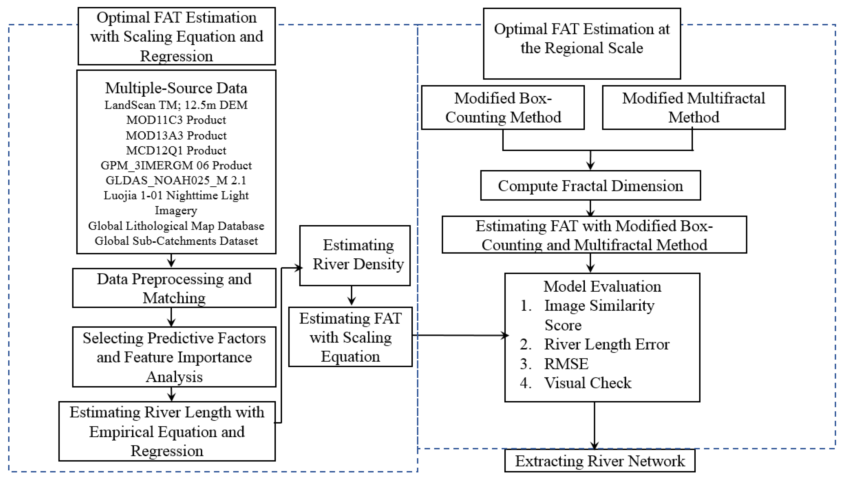
2. Methodology
2.1. The Estimation of the FAT with Empirical Scaling Equation and Statistical Regression at the Basin Scale
2.1.1. Empirical Scaling Equation Relating the Drainage Density and the FAT
2.1.2. Estimation of the River Length
2.1.3. NMF
2.2. The Estimation of the FAT at the Regional Scale
2.2.1. The Box-Counting Method
2.2.2. The Multifractal Method
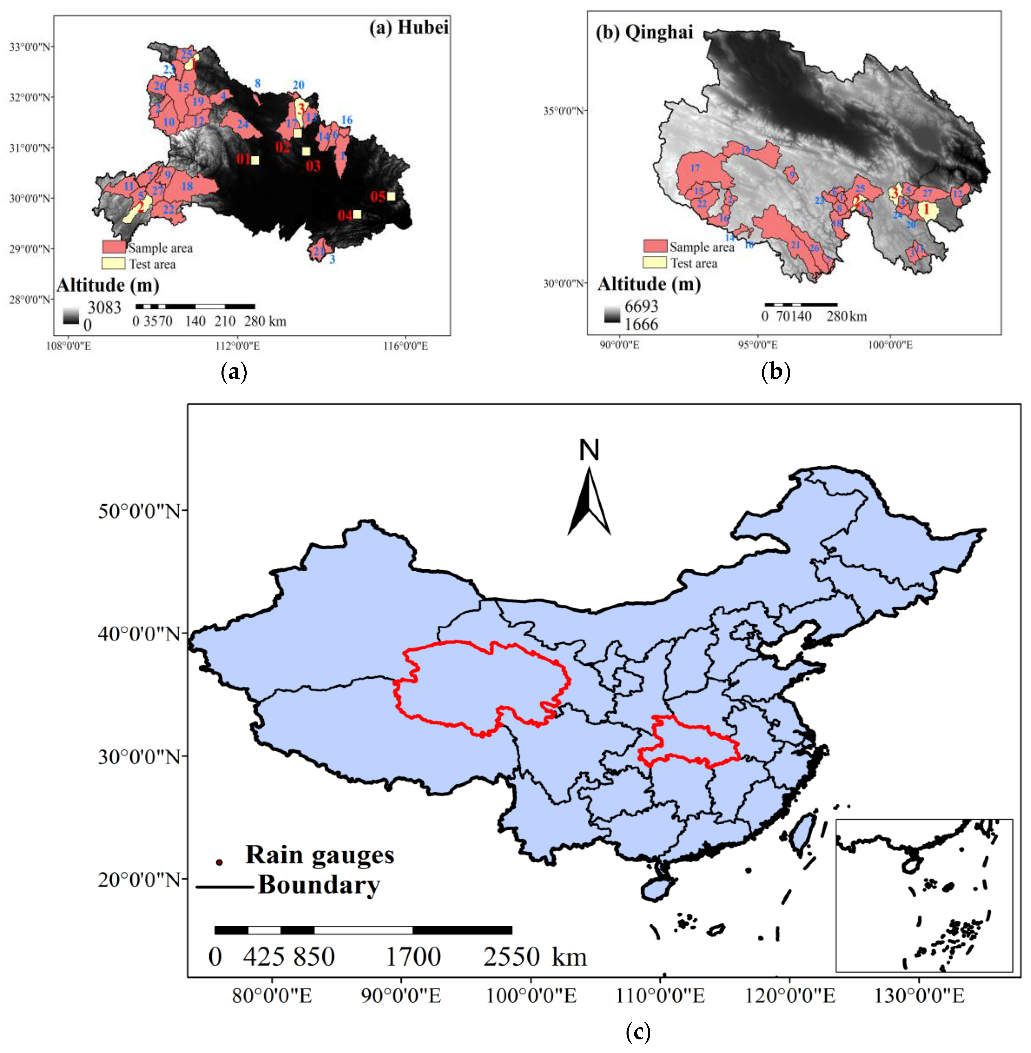
2.3. Study Area and Original Data
2.4. Data Pre-Processing and Normalization
2.5. Sample and Test Areas
2.6. Validation Method
3. Results and Discussion
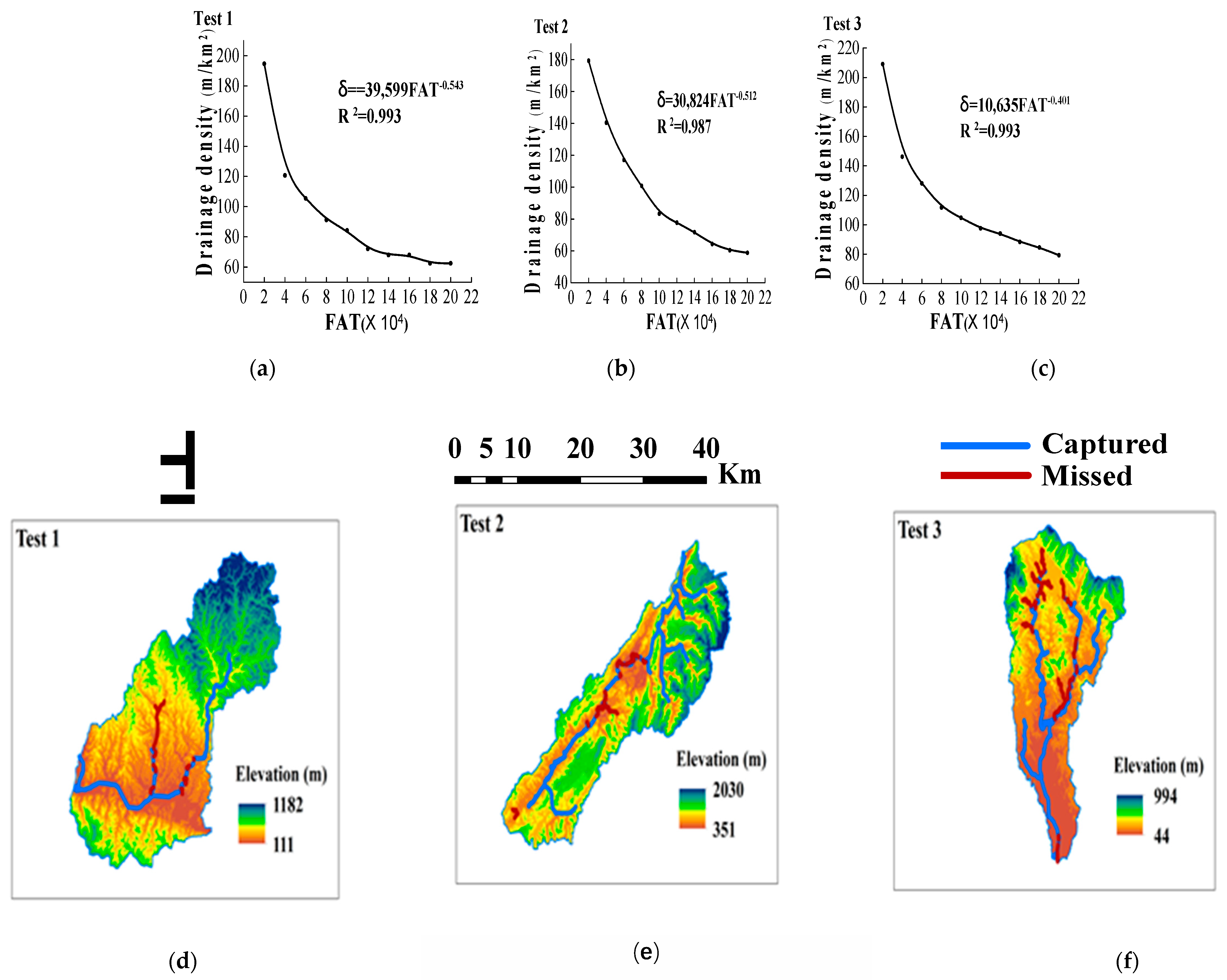
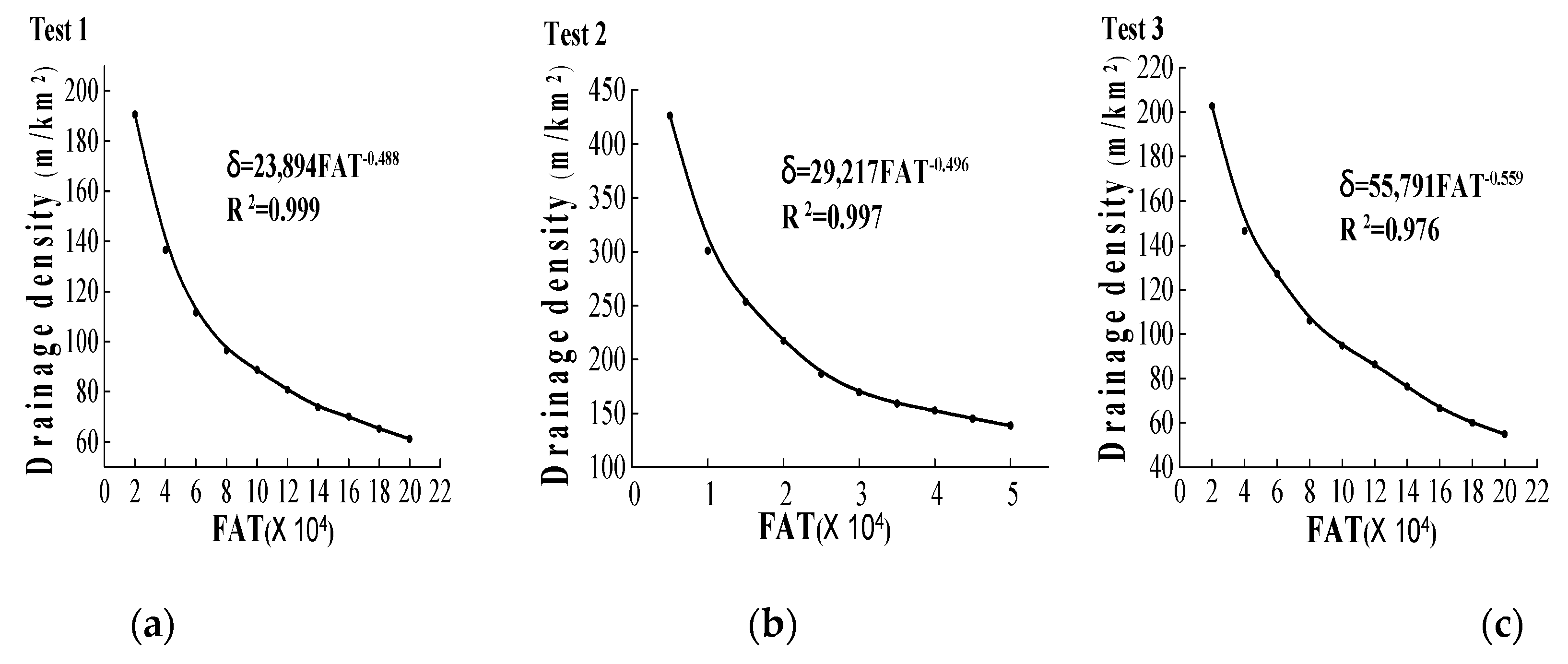
3.1. Estimation of the FAT by Empirical Scaling Equation and Statistical Regression at the Basin Scale
3.1.1. Estimation of the River Length
3.1.2. Estimating the FAT
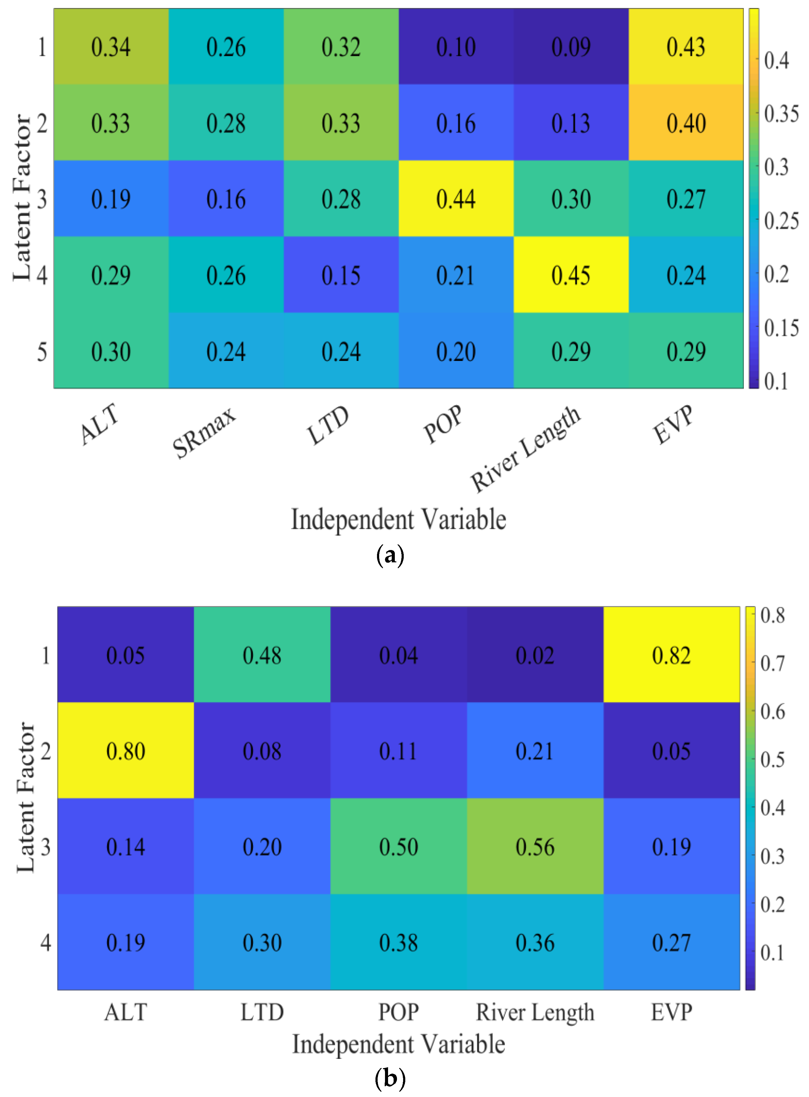
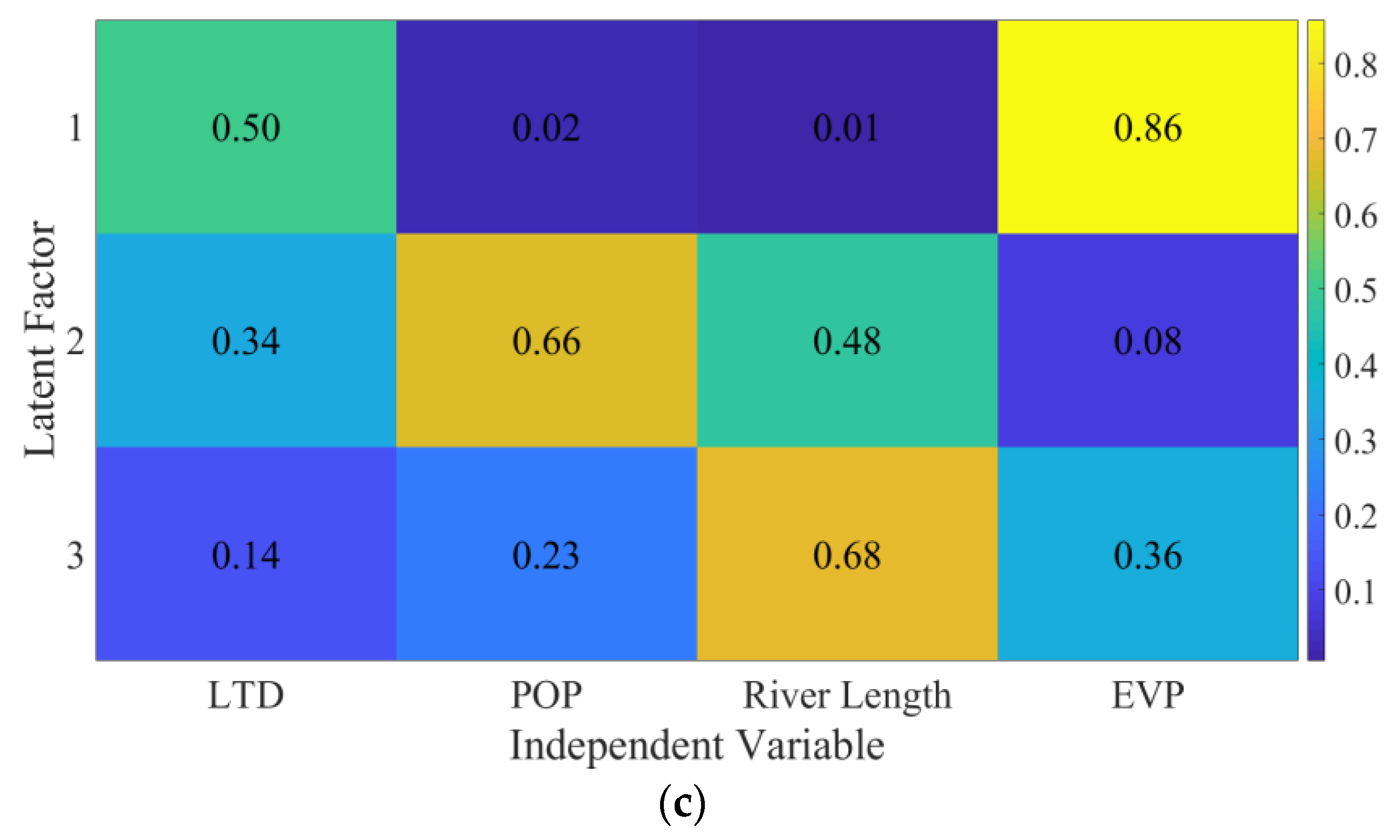
3.1.3. NMF
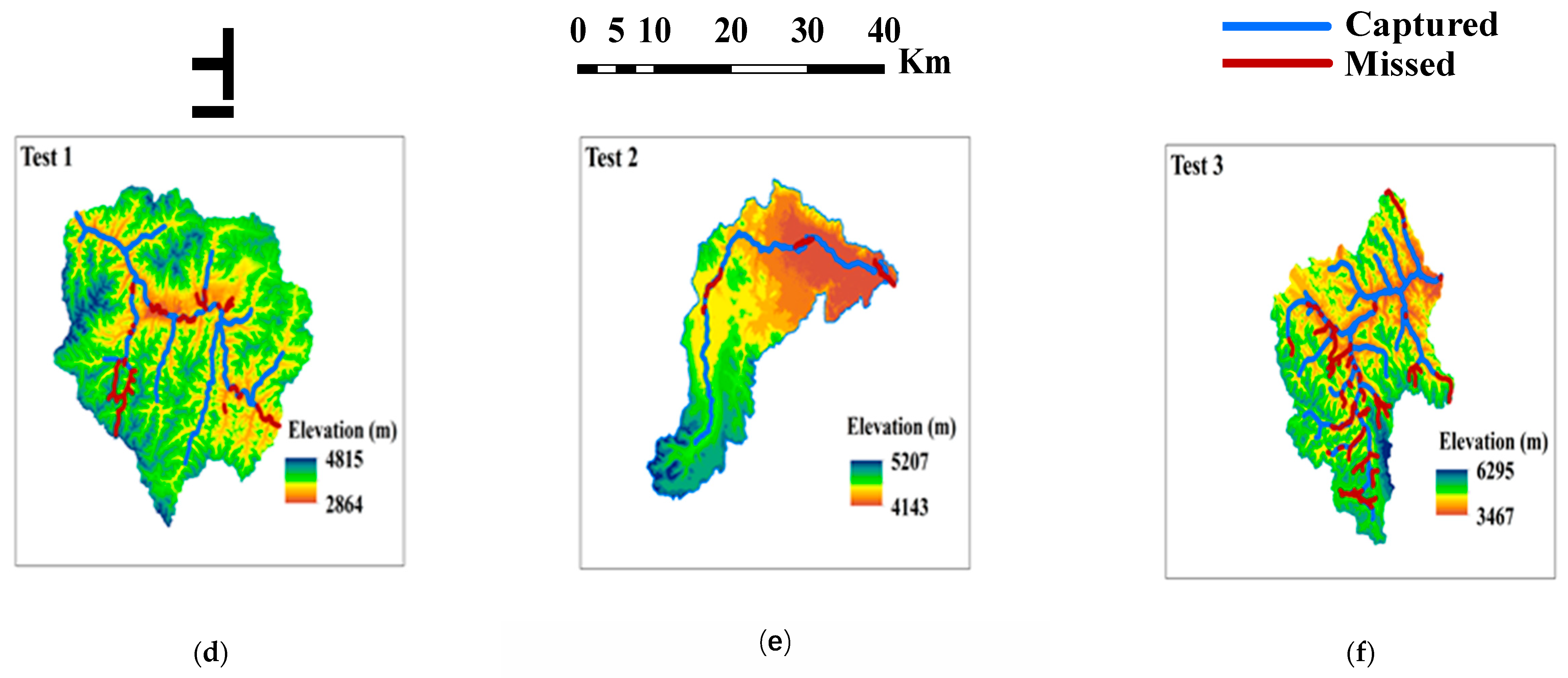
3.1.4. Validation
3.2. Estimation of the FAT at the Regional Scale (Hubei Province)
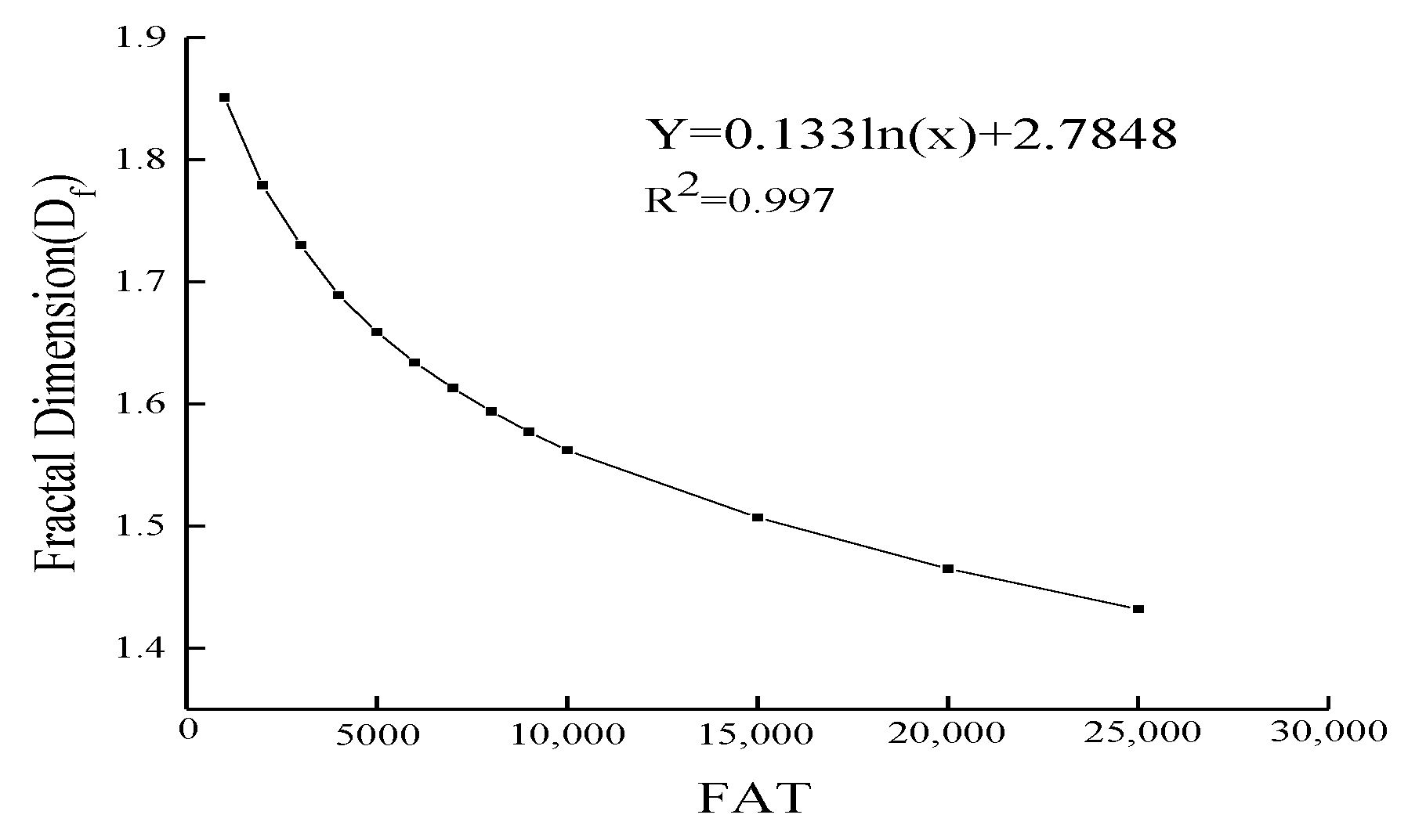
3.2.1. Estimation of the Optimal FAT with the Box-Counting Method
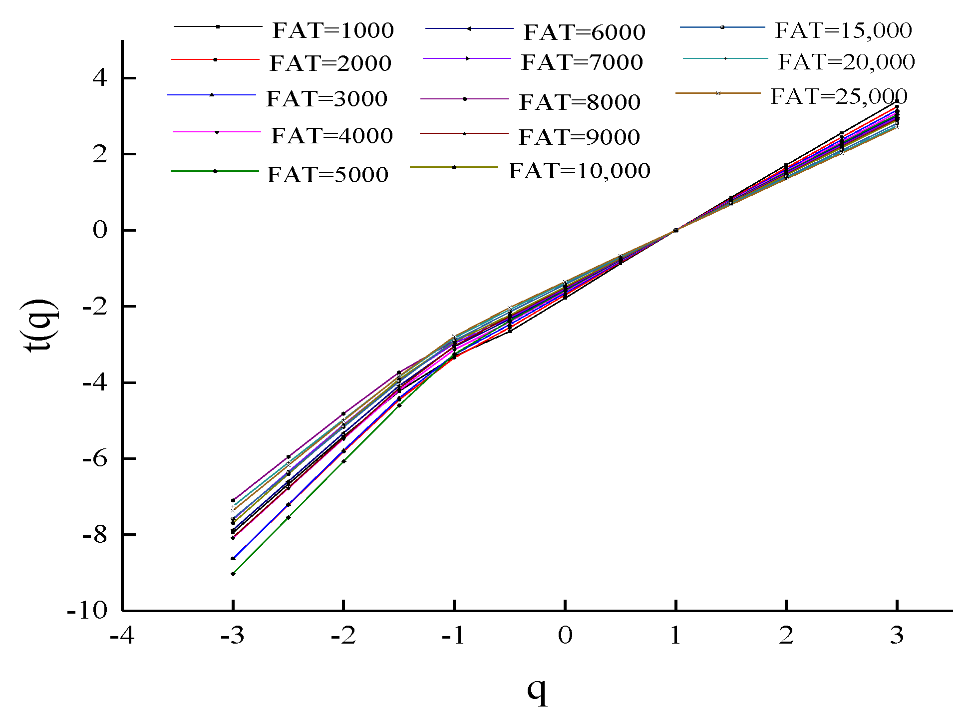
3.2.2. Estimation of the Optimal FAT with Multifractal Analysis
3.2.3. Validation
- (1)
- Similarity score
- (2)
- River length error
3.3. Discussion
4. Conclusions
Supplementary Materials
Author Contributions
Funding
Institutional Review Board Statement
Informed Consent Statement
Data Availability Statement
Acknowledgments
Conflicts of Interest
References
- Yang, B.; Ren, L.L. Identification and comparison of critical support area in extracting drainage network from DEM. Water Resour. Power 2009, 27, 11–14. [Google Scholar]
- Lindsay, J.B.; Dhun, K. Modelling surface drainage patterns in altered landscapes using LiDAR. Int. J. Geogr. Inf. Sci. 2015, 29, 397–411. [Google Scholar] [CrossRef]
- Ariza-Villaverde, A.B.; Jimenez-Hornero, F.J.; De Ravé, E.G. Multifractal analysis applied to the study of the accuracy of DEM-based stream derivation. Geomorphology 2013, 197, 85–95. [Google Scholar] [CrossRef]
- Garneau, C.; Sauvage, S.; Sánchez-Pérez, J.M.; Lofts, S.; Brito, D.; Neves, R.; Probst, A. Modelling trace metal transfer in large rivers under dynamic hydrology: A coupled hydrodynamic and chemical equilibrium model. Environ. Model. Softw. 2017, 89, 77–96. [Google Scholar] [CrossRef] [Green Version]
- Obida, C.B.; Blackburn, G.A.; Whyatt, J.D.; Semple, K.T. River network delineation from Sentinel-1 SAR data. Int. J. Appl. Earth Obs. Geoinform. 2019, 83. [Google Scholar] [CrossRef]
- Wu, T.; Li, J.; Li, T.; Sivakumar, B.; Zhang, G.; Wang, G. High-efficient extraction of drainage networks from digital elevation models constrained by enhanced flow enforcement from known river maps. Geomorphology 2019, 340, 184–201. [Google Scholar] [CrossRef]
- Montgomery, D.R.; Dietrich, W.E. Where do channels begin? Nat. Cell Biol. 1988, 336, 232–234. [Google Scholar] [CrossRef]
- Montgomery, D.R.; Dietrich, W.E. Channel Initiation and the Problem of Landscape Scale. Science 1992, 255, 826–830. [Google Scholar] [CrossRef] [Green Version]
- Passalacqua, P.; Trung, T.D.; Foufoula-Georgiou, E.; Sapiro, G.; Dietrich, W.E. A geometric framework for channel network extraction from lidar: Nonlinear diffusion and geodesic paths. J. Geophys. Res. Space Phys. 2010, 115, 01002. [Google Scholar] [CrossRef] [Green Version]
- Sangireddy, H.; Stark, C.P.; Kladzyk, A.; Passalacqua, P. GeoNet: An open source software for the automatic and objective extraction of channel heads, channel network, and channel morphology from high resolution topography data. Environ. Model. Softw. 2016, 83, 58–73. [Google Scholar] [CrossRef] [Green Version]
- Freeman, T. Calculating catchment area with divergent flow based on a regular grid. Comput. Geosci. 1991, 17, 413–422. [Google Scholar] [CrossRef]
- Lea, N.L. An aspect driven kinematic routing algorithm. In Overland Flow: Hydraulics and Erosion Mechanics; Chapman and Hall: New York, NY, USA, 1992. [Google Scholar]
- Costa-Cabral, M.C.; Burges, S.J. Digital Elevation Model Networks (DEMON): A model of flow over hillslopes for computation of contributing and dispersal areas. Water Resour. Res. 1994, 30, 1681–1692. [Google Scholar] [CrossRef]
- Tarboton, D.G. A new method for the determination of flow directions and upslope areas in grid digital elevation models. Water Resour. Res. 1997, 33, 309–319. [Google Scholar] [CrossRef] [Green Version]
- Orlandini, S.; Moretti, G.; Franchini, M.; Aldighieri, B.; Testa, B. Path-based methods for the determination of nondispersive drainage directions in grid-based digital elevation models. Water Resour. Res. 2003, 39, 1144. [Google Scholar] [CrossRef] [Green Version]
- Li, J.; Li, T.; Zhang, L.; Sivakumar, B.; Fu, X.; Huang, Y.; Bai, R. A D8-compatible high-efficient channel head recognition method. Environ. Model. Softw. 2020, 125, 104624. [Google Scholar] [CrossRef]
- Ibrahim, M.O.; Türkay, G. Examining the stream threshold approaches used in hydrologic analysis. Int. J. Geo.-Inf. 2018, 7, 201. [Google Scholar]
- Tarboton, D.G.; Bras, R.L.; Rodriguez-Iturbe, I. On the extraction of channel networks from digital elevation data. Hydrol. Process. 1991, 5, 81–100. [Google Scholar] [CrossRef]
- Lin, W.T.; Chou, W.C.; Lin, C.Y.; Huang, P.H.; Tsai, J.S. Automated suitable drainage network extraction from digital elevation models in Taiwan’s up-stream watersheds. Hydrol. Proc. 2006, 20, 289–306. [Google Scholar] [CrossRef]
- Oliveira, F. Arc Hydro: GIS for Water Resources; Maidment, D.R., Ed.; ESRI, Inc.: Redlands, CA, USA, 2002; Volume 1, pp. 55–86. [Google Scholar]
- Tang, G. A Research on the Accuracy of Digital Elevation Models; Science Press: Beijing, China, 2000. [Google Scholar]
- Jones, R. Algorithms for using a DEM for mapping catchment areas of stream sediment samples. Comput. Geosci. 2002, 28, 1051–1060. [Google Scholar] [CrossRef]
- Tantasirin, C.; Nagai, M.; Tipdecho, T.; Tripathi, N.K. Reducing hillslope size in digital elevation models at various scales and the effects on slope gradient estimation. Geocarto Int. 2016, 31, 140–157. [Google Scholar] [CrossRef]
- Gökgöz, T.; Ulugtekin, N.; Basaraner, M.; Gulgen, F.; Dogru, A.O.; Bilgi, S.; Yucel, M.A.; Cetinkaya, S.; Selcuk, M.; Ucar, D. Watershed delineation from grid DEMs in GIS: Effects of drainage lines and resolution. In Proceedings of the 10th International Specialised Conference on Diffuse Pollution and Sustainable Basin Management, Istanbul, Turkey, 18–22 September 2006. [Google Scholar]
- Vogt, J.V.; Colombo, R.; Bertolo, F. Deriving drainage networks and catchment boundaries: A new methodology combining digital elevation data and environmental characteristics. Geomophology 2003, 53, 281–298. [Google Scholar] [CrossRef]
- Camporeale, C.V.; Perucca, E.; Ridolfi, L.; Gurnell, A.M. Modeling the Interactions between River Morphodynamics and Riparian Vegetation. Rev. Geophys. 2013, 51, 379–414. [Google Scholar] [CrossRef] [Green Version]
- Kirkby, M.J. Long term interactions between networks and hillslopes. In Channel Network Hydrology; Beven, K., Kirkby, M.J., Eds.; John Wiley: New York, NY, USA, 1993; pp. 255–393. [Google Scholar]
- Horton, R.E. Drainage-basin characteristics. Trans. Am. Geophys. Union 1932, 13, 350–361. [Google Scholar] [CrossRef]
- Luo, W.; Jasiewicz, J.; Stepinski, T.; Wang, J.; Xu, C.; Cang, X. Spatial association between dissection density and environmental factors over the entire contermi-nous United States. Geophys. Res. Lett. 2016, 43, 692–700. [Google Scholar] [CrossRef] [Green Version]
- Schneider, A.; Jost, A.; Coulon, C.; Silvestre, M.; Théry, S.; Ducharne, A. Global-scale river network extraction based on high-resolution topography and constrained by lithology, climate, slope, and observed drainage density. Geophys. Res. Lett. 2017, 44, 2773–2781. [Google Scholar] [CrossRef] [Green Version]
- Strohbach, M.W.; Haase, D. Above-ground carbon storage by urban trees in Leipzig, Germany: Analysis of patterns in a European city. Landsc. Urban Plan. 2012, 104, 95–104. [Google Scholar] [CrossRef]
- Chi, Y.; Shi, H.; Zheng, W.; Sun, J.; Fu, Z. Spatiotemporal characteristics and ecological effects of the human interference index of the Yellow River Delta in the last 30 years. Ecol. Indic. 2018, 89, 880–892. [Google Scholar] [CrossRef]
- Song, S.; Zeng, L.; Wang, Y.; Li, G.; Deng, X. The response of river network structure to urbanization: A multifractal perspective. J. Clean. Prod. 2019, 221, 377–388. [Google Scholar] [CrossRef]
- Shao, X.; Fang, Y.; Cui, B. A model to evaluate spatiotemporal variations of hydrological connectivity on a basin-scale complex river network with intensive human activity. Sci. Total Environ. 2020, 723, 138051. [Google Scholar] [CrossRef]
- Chen, Y.; Xu, Y.; Fu, W. Influences of urbanization on river network in the coastal areas of East Zhejiang province. Adv. Water Sci. 2007, 18, 73. [Google Scholar]
- Benstead, J.P.; Leigh, D.S. An expanded role for river networks. Nat. Geosci. 2012, 5, 678–679. [Google Scholar] [CrossRef]
- Persendt, F.; Gomez, C. Assessment of drainage network extractions in a low-relief area of the Cuvelai Basin (Namibia) from multiple sources: LiDAR, topographic maps, and digital aerial orthophotographs. Geomorphology 2016, 260, 32–50. [Google Scholar] [CrossRef] [Green Version]
- Hou, J.W.; van Dijk, A.I.J.M.; Beck, H.E. Global satellite-based river gauging and the influence of river morphology on its application. Remote Sens. Environ. 2020, 239, 11629. [Google Scholar] [CrossRef]
- Farr, T.G.; Rosen, P.A.; Caro, E.; Crippen, R.; Duren, R.; Hensley, S.; Kobrick, M.; Paller, M.; Rodriguez, E.; Roth, L.; et al. The Shuttle Radar Topography Mission. Rev. Geophys. 2007, 45. [Google Scholar] [CrossRef] [Green Version]
- Ariza-Villaverde, A.; Jiménez-Hornero, F.; De Ravé, E.G. Influence of DEM resolution on drainage network extraction: A multifractal analysis. Geomorphology 2015, 241, 243–254. [Google Scholar] [CrossRef]
- Woodrow, K.; Lindsay, J.B.; Berg, A.A. Evaluating DEM conditioning techniques, elevation source data, and grid resolution for field-scale hydrological parameter extraction. J. Hydrol. 2016, 540, 1022–1029. [Google Scholar] [CrossRef]
- Niipele, J.N.; Chen, J.P. The usefulness of also-palsar dem data for drainage extraction in semi-arid environments in The Iishana sub-basin. J. Hydrol. Reg. Stud. 2019, 21, 57–67. [Google Scholar] [CrossRef]
- Colombo, R.; Vogt, J.V.; Soille, P.; Paracchini, M.L.; de Jager, A. Deriving river networks and catchments at the European scale from medium resolution digital elevation data. Catena 2007, 70, 296–305. [Google Scholar] [CrossRef]
- Mandelbrot, B.B. The Fractal Geometry of Nature/Revised and Enlarged Edition; WH Freeman and Co.: New York, NY, USA, 1983; 49p. [Google Scholar]
- Shen, X.; Zou, L.; Zhang, G.; Su, N.; Wu, W.; Yang, S. Fractal characteristics of the main channel of Yellow River and its relation to regional tectonic evolution. Geomorphology 2011, 127, 64–70. [Google Scholar] [CrossRef]
- Joanna, F.B. Fractal structure of the Kashubian hydrographic system. J. Hydrol. 2013, 488, 48–54. [Google Scholar]
- Zhang, S.; Guo, Y.; Wang, Z. Correlation between flood frequency and geomorphologic complexity of rivers network—A case study of Hangzhou China. J. Hydrol. 2015, 527, 113–118. [Google Scholar] [CrossRef] [Green Version]
- Bai, R.; Li, T.; Huang, Y.; Li, J.; Wang, G. An efficient and comprehensive method for drainage network extraction from DEM with billions of pixels using a size-balanced binary search tree. Geomorphology 2015, 238, 56–67. [Google Scholar] [CrossRef]
- O’Callaghan, J.F.; Mark, D.M. The extraction of drainage networks from digital elevation data. Comput. Vis. Graph. Image Process. 1984, 28, 323–344. [Google Scholar] [CrossRef]
- Lee, D.D.; Seung, H.S. Learning the parts of objects by non-negative matrix factorization. Nat. Cell Biol. 1999, 401, 788–791. [Google Scholar] [CrossRef]
- Zhang, H.; Loáiciga, H.; Ren, F.; Du, Q.; Ha, D. Semi-empirical prediction method for monthly precipitation prediction based on environmen-tal factors and comparison with stochastic and machine learning models. Hydrol. Sci. J. 2020, 65, 1–15. [Google Scholar] [CrossRef]
- De Bartolo, S.G.; Gaudio, R.; Gabriele, S. Multifractal analysis of river networks: Sandbox approach. Water Resour. Res. 2004, 40, 02201. [Google Scholar] [CrossRef] [Green Version]
- Grassberger, P. On Efficient Box Counting Algorithms. Int. J. Mod. Phys. C 1993, 4, 515–523. [Google Scholar] [CrossRef]
- Ge, M.; Lin, Q. Realizing the box-counting method for calculating fractal dimension of urban form based on remote sensing image. Geo.-Spatial. Inf. Sci. 2009, 12, 265–270. [Google Scholar] [CrossRef] [Green Version]
- Pavón-Domínguez, P.; Rincón-Casado, A.; Ruiz, P.; Camacho-Magriñán, P. Multifractal approach for comparing road transport network geometry: The case of Spain. Phys. A Stat. Mech. Appl. 2018, 510, 678–690. [Google Scholar] [CrossRef]
- Halsey, T.C.; Jensen, M.H.; Kadanoff, L.P.; Procaccia, I.; Shraiman, B.I. Fractal measures and their singularities: The characterization of strange sets. Phys. Rev. A 1986, 33, 1141–1151. [Google Scholar] [CrossRef]
- Chakraborty, B.; Haris, K.; Latha, G.; Maslov, N.; Menezes, A. Multifractal Approach for Seafloor Characterization. IEEE Geosci. Remote Sens. Lett. 2013, 11, 54–58. [Google Scholar] [CrossRef]
- Ge, Y.; Dou, W.; Gu, Z.; Qian, X.; Wang, J.; Xu, W.; Shi, P.; Ming, X.; Zhou, X.; Chen, Y. Assessment of social vulnerability to natural hazards in the Yangtze River Delta, China. Stoch. Environ. Res. Risk Assess. 2013, 27, 1899–1908. [Google Scholar] [CrossRef]
- Zhang, H.; Loáiciga, H.A.; Ha, D.; Du, Q. Spatial and Temporal Downscaling of TRMM Precipitation with Novel Algorithms. J. Hydrometeorol. 2020, 21, 1259–1278. [Google Scholar] [CrossRef]
- Wang, R.; Li, C. Spatiotemporal analysis of precipitation trends during 1961–2010 in Hubei province, central China. Theor. Appl. Clim. 2016, 124, 385–399. [Google Scholar] [CrossRef]
- Gregory, K.J.; Gardiner, V. Drainage density and climate. Geomorphology 1975, 19, 287–298. [Google Scholar]
- Moglen, G.E.; Eltahir, E.A.B.; Bras, R.L. On the sensitivity of drainage density to climate change. Water Resour. Res. 1998, 34, 855–862. [Google Scholar] [CrossRef] [Green Version]
- Yang, H.-L.; Xiao, H.; Guo, C.; Sun, Y. Spatial-temporal analysis of precipitation variability in Qinghai Province, China. Atmos. Res. 2019, 228, 242–260. [Google Scholar] [CrossRef]
- Yan, D.; Wang, K.; Qin, T.; Weng, B.; Wang, H.; Bi, W.; Li, X.; Li, M.; Lv, Z.; Liu, F.; et al. A data set of global river networks and corresponding water resources zones divisions. Sci. Data 2019, 6, 1–11. [Google Scholar] [CrossRef] [PubMed] [Green Version]
- Han, X.; Fang, W.; Li, H.; Wang, Y.; Shi, J. Heterogeneity of influential factors across the entire air quality spectrum in Chinese cities: A spatial quantile regression analysis. Environ. Pollut. 2020, 262, 114259. [Google Scholar] [CrossRef]
- Hartmann, J.; Moosdorf, N. The new global lithological map database GLiM: A representation of rock proper-ties at the Earth surface. Geochem. Geophys. Geosyst. 2012, 13, Q12004. [Google Scholar] [CrossRef]
- Jenness, J.S. Calculating landscape surface area from digital elevation models. Wildl. Soc. Bull. 2004, 32, 829–839. [Google Scholar] [CrossRef]
- Hodgson, M.E.; Gaile, G.L. A cartographic modeling approach for surface orientation-related applications. Photogramm. Eng. Remote Sens. 1999, 65, 85–95. [Google Scholar]
- Grohmann, C.H.; Smith, M.J.; Riccomini, C. Multi-scale analysis of topographic surface roughness in the mid-land valley, Scotland. IEEE Trans. Geosci. Remote Sens. 2011, 49, 1200–1213. [Google Scholar] [CrossRef] [Green Version]
- Lindsay, J.B.; Newman, D.R.; Francioni, A. Scale-Optimized Surface Roughness for Topographic Analysis. Geoscience 2019, 9, 322. [Google Scholar] [CrossRef] [Green Version]
- Feng, H.; Zou, B.; Tang, Y. Scale- and Region-Dependence in Landscape-PM2.5 Correlation: Implications for Urban Planning. Remote Sens. 2017, 9, 918. [Google Scholar] [CrossRef] [Green Version]
- Wang, C.; Chen, Z.; Yang, C.; Li, Q.; Wu, Q.; Wu, J.; Zhang, G.; Yu, B. Analyzing parcel-level relationships between Luojia 1-01 nighttime light intensity and artificial surface features across Shanghai, China: A comparison with NPP-VIIRS data. Int. J. Appl. Earth Obs. Geoinform. 2020, 85, 101989. [Google Scholar] [CrossRef]
- Zou, L. On a conjecture concerning the Frobenius norm of matrices. Linear Multilinear Algebra 2012, 60, 27–31. [Google Scholar] [CrossRef]
- Yang, Y.Z.; Cai, W.H.; Yang, J. Evaluation of MODIS Land Surface Temperature Data to Estimate Near-Surface Air Temperature in Northeast China. Remote Sens. 2017, 9, 410. [Google Scholar] [CrossRef] [Green Version]
- Cui, X.; Zhang, J.; Wu, X.; Hao, N.; Wang, Q. Dynamic Change of Land Cover of Qinling Mountains Based on MODIS NDVI. In Proceedings of the 2018 Fifth International Workshop on Earth Observation and Remote Sensing Applications (EORSA), Xi’an, China, 18–20 June 2018; pp. 1–5. [Google Scholar]
- Kohavi, R. A study of cross-validation and bootstrap for accuracy estimation and model selection. In Proceedings of the Fourteenth International Joint Conference on Artificial Intelligence, Montreal, QC, Canada, 20–25 August 1995; Volume 2, pp. 1137–1143. [Google Scholar]
- He, L.H.; Zhao, H. The fractal dimension of river networks and its interpretation. Sci. Geogr. Sin. 1996, 2, 124–128. (In Chinese) [Google Scholar]
- Martz, L.W.; Garbrecht, J. Numerical definition of drainage network and subcatchment areas from Digital Elevation Models. Computer Geosci. 1992, 18, 747–761. [Google Scholar] [CrossRef]
- Stein, J.L.; Hutchinson, M.F. A new stream and nested catchment framework for Australia. Hydrol. Earth Syst. Sci. 2014, 18, 1917–1933. [Google Scholar] [CrossRef] [Green Version]
- Yao, Q.; Liu, K.-B.; Aragón-Moreno, A.A.; Rodrigues, E.; Xu, Y.J.; Lam, N.S. A 5200-year paleoecological and geochemical record of coastal environmental changes and shoreline fluctuations in southwestern Louisiana: Implications for coastal sustainability. Geomorphology 2020, 365, 107284. [Google Scholar] [CrossRef]


| Category | Brief Description | Year | Symbol | Unit |
|---|---|---|---|---|
| Meteorological factors | Average monthly precipitation | 2001–2018 (5–9) | PRE | Mm |
| Average monthly surface runoff | 2001–2018 (5–9) | ROF | Mm | |
| Average monthly evapotranspiration | 2001–2018 (5–9) | EVP | Mm | |
| Average surface temperature | 2001–2018 (5–9) | LTD | °C | |
| Topographical factors | Maximum terrain altitude | 2018 | ALTmax | M |
| Mean terrain altitude | 2018 | M | ||
| Maximum slope | 2018 | SLPmax | ° | |
| Mean slope | 2018 | ° | ||
| Maximum surface roughness | 2018 | SRmax | / | |
| Mean surface roughness | 2018 | / | ||
| Vegetation factors | Normalized Difference Vegetation Index | 2001–2018 (5–9) | NDVI | / |
| Anthropogenic factors | Population ratio | 2018 | Q | % |
| Basin light area | 2018 | L1 | / | |
| Basin light intensity | 2018 | L2 | / | |
| Landscape factors | Landscape percentage | 2018 | PLAND | % |
| Shannon’s diversity index | 2018 | SHDI | % | |
| Species evenness | 2018 | SEI | % | |
| Patch density | 2018 | PD | number/ km2 | |
| Lithology factors | Lithology type | 2012 | LT | / |
| Ranking | Drainage Density δ (m/km2) | Dominant Rock Type | Ranking | Drainage Density δ (m/km2) | Dominant Rock Type |
|---|---|---|---|---|---|
| 1 | 246.922 | sc, su | 15 | 119.891 | Mt |
| 2 | 230.128 | Su | 16 | 118.144 | Sm |
| 3 | 228.912 | Sc | 17 | 115.381 | Sm |
| 4 | 221.086 | Sm | 18 | 113.214 | Sm |
| 5 | 191.177 | Sc | 19 | 104.364 | su, sm |
| 6 | 158.465 | su, ss | 20 | 97.355 | Sm |
| 7 | 145.309 | Py | 21 | 95.585 | sm, sc |
| 8 | 145.045 | sm, sc | 22 | 93.063 | Sm |
| 9 | 144.632 | sm, sc | 23 | 91.383 | su, ss, pa |
| 10 | 144.534 | Pa | 24 | 89.913 | su, py |
| 11 | 139.167 | Sm | 25 | 83.102 | Sm |
| 12 | 135.286 | sm, sc | 26 | 73.790 | Py |
| 13 | 133.594 | sm, sc | 27 | 53.544 | Sm |
| 14 | 122.085 | Sm |
| Area | Actual River Length (m) | Estimated River Length (m) see Equation (21) | FATs | Extracted River Length (m) | River Length Error (%) | SSEI |
|---|---|---|---|---|---|---|
| 1 | 62,109 | 61,323 | 101,237 | 60,050 | 1.17 | 0.441 |
| 2 | 151,113 | 161,006 | 80,916 | 169,379 | 10.34 | 0.356 |
| 3 | 176,724 | 176,287 | 54,547 | 171,143 | 3.16 | 0.400 |
| Average | 4.89% |
| Area | Actual River Length (m) | Estimated River Length (m) see Equation (21) | FATs | Extracted River Length (m) | River Length Error (%) | SSEI |
|---|---|---|---|---|---|---|
| 1 | 302,294 | 322,167 | 190,275 | 291,539 | 3.56 | 0.622 |
| 2 | 95,765 | 127,176 | 140,641 | 119,354 | 24.63 | 0.583 |
| 3 | 429,522 | 409,901 | 41,356 | 403,155 | 6.14 | 0.478 |
| Average | 11.44% |
| Method | FAT | Length Error (%) | Accuracy |
|---|---|---|---|
| drainage density-FAT | 140,641 | 24.63 | High |
| Fitness index | 135,000 | 25.44 | High |
| OnePercent | 18,840 | 87.96 | Low |
| Mean | 1908 | 504.06 | Very Low |
| FAT | Fractal Dimension (Df) | R2 | Change Rate (di) | FAT | Fractal Dimension (Df) | R2 | Change Rate (di) |
|---|---|---|---|---|---|---|---|
| 1000 | 1.851 | 0.999 | 0.0072 | 8000 | 1.594 | 0.994 | 0.0017 |
| 2000 | 1.779 | 0.997 | 0.0049 | 9000 | 1.577 | 0.994 | 0.0015 |
| 3000 | 1.730 | 0.996 | 0.0041 | 10,000 | 1.562 | 0.993 | 0.0011 |
| 4000 | 1.689 | 0.995 | 0.003 | 15,000 | 1.507 | 0.994 | 0.00084 |
| 5000 | 1.659 | 0.995 | 0.0025 | 20,000 | 1.465 | 0.994 | 0.00066 |
| 6000 | 1.634 | 0.994 | 0.0021 | 25,000 | 1.432 | 0.994 | |
| 7000 | 1.613 | 0.994 | 0.0019 |
| FAT | (1) | (2) | (3) | (4) | (5) | (6) |
|---|---|---|---|---|---|---|
| 1000 | 1.448 | 0.951 | 2.209 | 1.317 | 0.761 | −0.366 |
| 2000 | 1.195 | 0.337 | 2.621 | 0.761 | 1.426 | −0.424 |
| 3000 | 1.109 | 0.167 | 2.671 | 0.614 | 1.562 | −0.447 |
| 4000 | 1.152 | 0.362 | 2.443 | 0.754 | 1.291 | −0.392 |
| 5000 | 0.935 | −0.239 | 2.937 | 0.209 | 2.002 | −0.448 |
| 6000 | 1.111 | 0.333 | 2.385 | 0.715 | 1.274 | −0.382 |
| 7000 | 1.125 | 0.408 | 2.264 | 0.807 | 1.139 | −0.399 |
| 8000 | 1.196 | 0.650 | 2.033 | 0.999 | 0.837 | −0.349 |
| 9000 | 0.995 | 0.071 | 2.535 | 0.467 | 1.540 | −0.396 |
| 10,000 | 1.034 | 0.208 | 2.351 | 0.635 | 1.317 | −0.427 |
| 15,000 | 0.989 | 0.162 | 2.357 | 0.506 | 1.368 | −0.344 |
| 20,000 | 0.998 | 0.250 | 2.228 | 0.565 | 1.230 | −0.315 |
| 25,000 | 0.926 | 0.077 | 2.310 | 0.433 | 1.384 | −0.356 |
| Test Area | Similarity Score (SSEI) | River Length Error (err(l)) (%) | ||
|---|---|---|---|---|
| Box-Counting Method | Multifractal Method | Box-Counting Method | Multifractal Method | |
| 01 | 1.0394 | 1.0334 | 21.49 | 16.49 |
| 02 | 1.0387 | 1.0395 | 20.13 | 18.42 |
| 03 | 1.2207 | 1.2202 | 26.53 | 20.15 |
| 04 | 1.0247 | 1.0223 | 36.46 | 29.26 |
| 05 | 1.3728 | 1.3674 | 26.28 | 22.90 |
Publisher’s Note: MDPI stays neutral with regard to jurisdictional claims in published maps and institutional affiliations. |
© 2021 by the authors. Licensee MDPI, Basel, Switzerland. This article is an open access article distributed under the terms and conditions of the Creative Commons Attribution (CC BY) license (http://creativecommons.org/licenses/by/4.0/).
Share and Cite
Zhang, H.; Loáiciga, H.A.; Feng, L.; He, J.; Du, Q. Setting the Flow Accumulation Threshold Based on Environmental and Morphologic Features to Extract River Networks from Digital Elevation Models. ISPRS Int. J. Geo-Inf. 2021, 10, 186. https://0-doi-org.brum.beds.ac.uk/10.3390/ijgi10030186
Zhang H, Loáiciga HA, Feng L, He J, Du Q. Setting the Flow Accumulation Threshold Based on Environmental and Morphologic Features to Extract River Networks from Digital Elevation Models. ISPRS International Journal of Geo-Information. 2021; 10(3):186. https://0-doi-org.brum.beds.ac.uk/10.3390/ijgi10030186
Chicago/Turabian StyleZhang, HuiHui, Hugo A. Loáiciga, LuWei Feng, Jing He, and QingYun Du. 2021. "Setting the Flow Accumulation Threshold Based on Environmental and Morphologic Features to Extract River Networks from Digital Elevation Models" ISPRS International Journal of Geo-Information 10, no. 3: 186. https://0-doi-org.brum.beds.ac.uk/10.3390/ijgi10030186