1. Introduction
Information extraction from 3D data has become an important field of research in photogrammetry, remote sensing, computer vision and robotics, with the increasing utility of 3-dimensional (3D) point clouds [
1]. Scanning an object with a laser generates 3D information about the shape of the object. This is the basic principle of creating depth perception for machines or 3D machine vision [
2]. Point clouds contain information such as 3D position information, density and color. The grouping of points with similar singular properties under a meaningful cluster is called classification. Problems of point cloud classification are insufficiency of existing databases, high hardware requirements for data processing and insufficient methods in terms of accuracy and speed.
Traditionally, point cloud classification relies on defining a set of discriminatory rules to distinguish points for each class [
3]. Although discriminatory rules are effective for controlled environments, methods still have inherent limitations when dealing with complex data involving uncertainty and complex relationships between classes. Therefore, point cloud classification for these complex data cannot be handled by combining simple decision rules. Machine learning is a powerful mathematical tool that can be used to classify complex point clouds. In machine learning algorithms, classification rules are learned automatically using training data instead of pre-determined arbitrary parameters. Machine learning and automatic feature selection avoid most of the tedious design and programming work involved in a traditional classification methodology. Thus, these methods are more convenient than traditional classification methods due to their effectiveness for complex data consisting of multiple object types [
4]. To accurately predict the semantic classification algorithms, the label of each point in the 3-dimensional point cloud and the geometry of the point cloud must be correctly defined [
5].
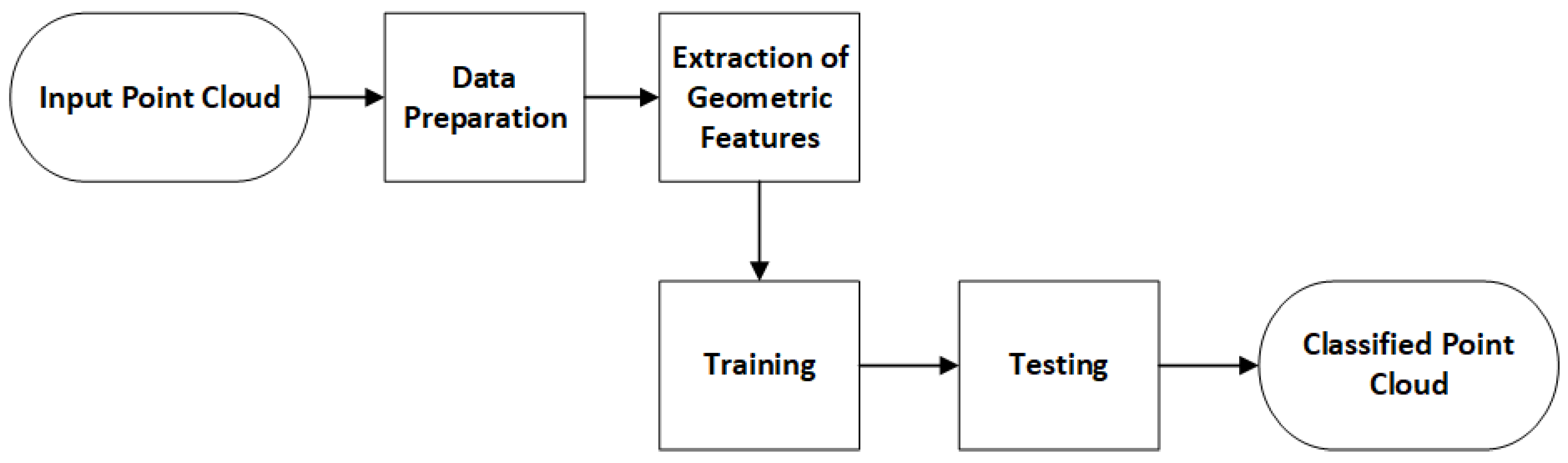
This study aims to examine the effects of geometric properties produced at different scales from point clouds on classification accuracy. A comprehensive examination has been realized to determine the support area size and to select the appropriate geometric features. It is aimed to better understand the classification performance of machine learning methods on point clouds of different densities and scales. The significance of geometric properties depending on the data and scale was examined. The datasets used in the study are the ISPRS 3D Semantic Labeling Contest Dataset of Vaihingen [
6], Dublin City [
7] and Oakland3D [
8] datasets. The support areas of each point of the point clouds were calculated in five different scales as 0.5 m, 1 m, 1.5 m, 2 m and 3 m, respectively. Two regions with different sizes of the Dublin dataset were selected for testing, whereas the entire test part of the Vaihingen dataset and Oakland3D dataset were used. In addition to the overall accuracy of the methods, precision, recall and F1 score values were also calculated for each class. Therefore, the effect of different support radii on the extraction of the classes has been examined in detail and the machine learning methods were compared. Algorithms chosen for comparison and evaluation are Random Forest (RF), Linear Discriminant Analysis (LDA), Gaussian Naïve Bayes (GNB), Logistic Regression (LR), Multi-Layer Perceptron (MLP), decision tree (DT), Support Vector Machines (SVM) and k-nearest neighbors (KNN). The effects of geometric features change depending on the support radius. To determine this change, feature importance was calculated with the RF method. The Python programming language and open-source Cloud Compare software were used in the study. Multi-scale point cloud classification has been carried out using popular machine learning algorithms cited in the literature. The utility of geometric features in point cloud supervised classification was investigated. The results obtained are presented in the form of tables and images. The flowchart of this applied approach is shown in
Figure 1.
2. Related Works
Supervised learning approaches that assign labels individually to each point in the point cloud can often be chosen. Weinmann et al. [
9] examined the use of different features for point cloud classification and the most appropriate support selection and different classifiers. The features that mostly affect the accuracy among produced features were determined by using feature selection methods. The Oakland 3D Point Cloud Dataset and Paris-rue-Lille Dataset, which are mobile laser scanning data, were used as the dataset. Random Forest was found to be the most effective classifier as a result of the evaluation. Vosselman et al. [
10] used 19 geometric features that were extracted from the point cloud in the study. In the proposed method, the point cloud was divided into certain groups and classified. The Vaihingen and Rotterdam datasets of International Society for Photogrammetry and Remote Sensing were used as the dataset. Conditional Random Field algorithm was selected as the classification method. Resultantly, group-based classification exerted better results than point-based classification. The landslide was investigated by using point clouds in [
11]. Objects were specified in the point cloud for object-based classification. Features were extracted from the point cloud to identify these objects. Classification was conducted via Support Vector Machines (SVM) and Random Forest (RO) methods using the extracted features. Seven classes were classified: landslide slope, eroded area, sediment, medium and high vegetation, small grasses, high grasses and rocks. In the study conducted by Belgui et al. [
12], the buildings were detected from the point cloud which was divided into three sub-classes; small buildings, apartment buildings and industrial buildings. In the study, the RF algorithm was trained using the features extracted from the point cloud. The extracted features were more related to height. Guo et al. [
4] proposed an ensemble-learning algorithm named JointBoost for point cloud classification. Ensemble methods aim to create a strong classifier by combining more than one weak classifier. In this study, five classes were classified as building, land, vegetation, power line and power line poles. 26 features were extracted from the point cloud for each point. The proposed approach had two stages. In the first stage, classification was realized with the JointBoost method by using the 17 most effective features. In the next stage, unreliable or misclassified points were again classified by the k-NN method. Landslide regions were determined in the point cloud in [
13]. For this purpose, Digital Terrain Model (DTM) produced the point cloud and aerial photographs were used. Firstly, 52 pixel-based features such as slope gradient, plan curvature, roughness and sky view factor were determined on DTM. These features were then transferred to the objects determined by Object-Based Image Analysis (OBIA). An RF-based feature selection algorithm was performed prior to classification because of the large number of features. RF and SVM algorithms were used as classifiers. The study proposed by Plaza-Leiva et al. [
14] focused on the efficiency of the spatial shape features obtained from the covariance analysis for improving computational load and accuracy of the supervised learning classification. For this purpose, eigenvalues were calculated for each point from the point cloud. The classification was based on three classes: city buildings, natural vegetation and artificial vegetation. Four different supervised learning algorithms were compared: SVM, artificial neural network, Gaussian operation and Gaussian mixing models. In [
15], a supervised classification was performed in both residential areas and forest areas. Five geometric properties were used from the point cloud: linearity, planarity, sphericity, horizontality and height change. SV machines, RF, logistic regression and linear discriminant analysis were chosen as classification algorithms. As a result of classifications with different support radius, an accuracy of approximately 80% for the residential area and 93% for the forest area has been obtained by using RF. In another study [
16], supervised classification of point clouds was done using geometric properties. In the study, four different datasets, including color information of points besides 15 geometric features, were used. Ground, high vegetation, building, road, car and human-made objects classes were extracted with RF and Boosted Tress methods. A photogrammetric point cloud was used for training and testing. In the Lin et al. [
3] study, the aerial point cloud was classified according to three geometric properties, namely linearity, planarity and sphericity, by using SVM. In the method proposed, it was aimed to increase the classification accuracy by weighting the covariance matrix. The targeted classes were divided into buildings and non-building structures.
As a powerful controlled statistical method, machine learning is the method that can be used to classify point clouds. When a point is defined by distinctive geometric properties, machine learning is used to predict the class of a point. Since the distinctiveness of geometric features is strongly dependent on the support areas of these 3D points considered for feature extraction, support area size and feature selection are important problems. With this study, it is evaluated that it can contribute to the gap about scale and feature selection in the literature. The effects of geometric properties obtained from different scales on current datasets were investigated. Some criteria based on results have been proposed for the choice of geometric feature and optimum support size.
3. Data and Methodology
3.1. Data Used
The proposed approach was evaluated for three different point cloud datasets of Dublin City, Vaihingen and Oakland3D that included urban areas. The Dublin data set was produced in 2015 by the Urban Modeling Group at University College Dublin (UCD) by scanning with ALS in Dublin City Center. 260 million out of 1.4 billion points have been labeled. The density of the point cloud varied from 250 to 348 points/m
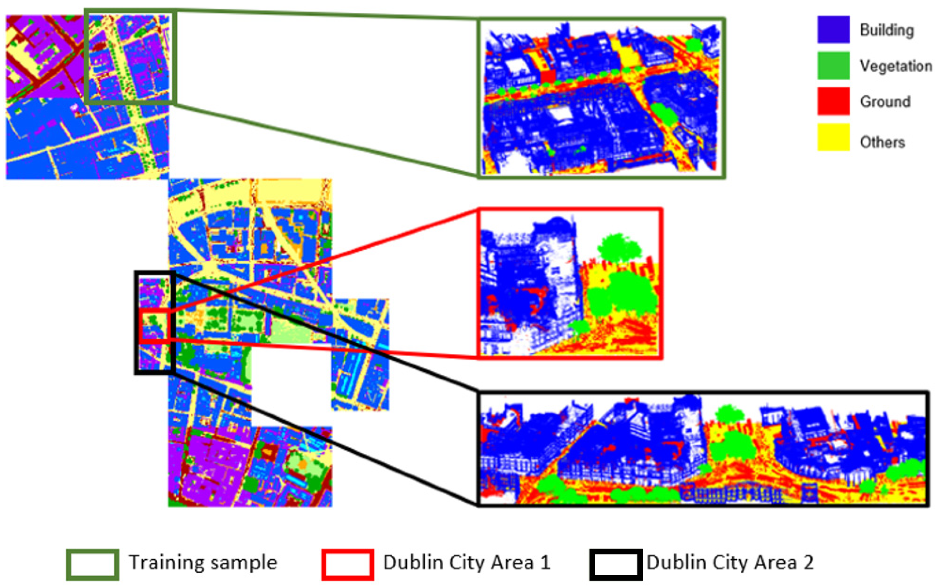
2. The point cloud consisted of 13 regions in total. In this study, since it was not possible to use the whole dataset due to hardware deficiencies, only two regions were selected and used. These two study regions covered approximately 20 million points. A training area (
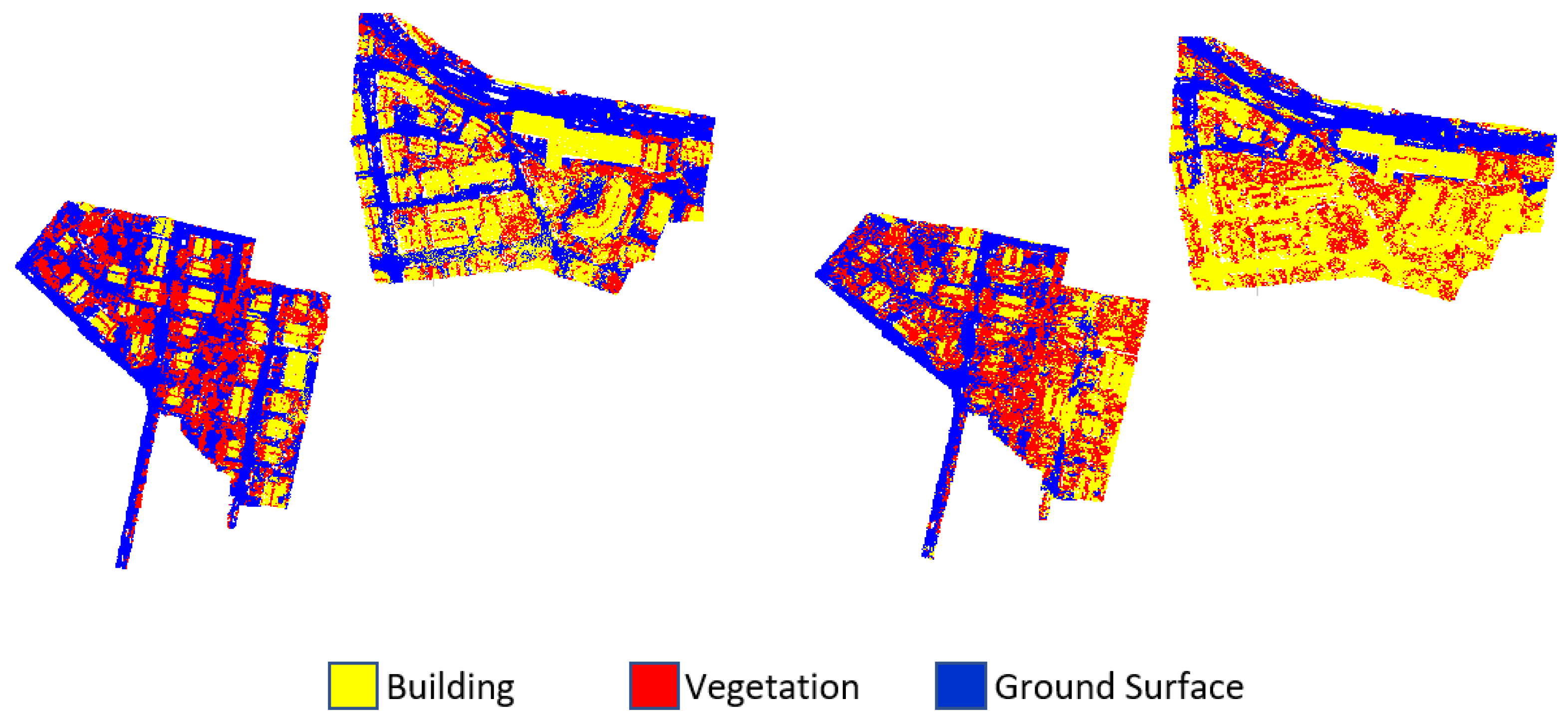
Figure 2) that covered approximately 12 million points was selected. In this area, points labeled as “undefined” were eliminated and for the rest of this process, 970,000 points were selected randomly from the dataset used for training to provide an advantage in efficiency and speed. Two test sites of Dublin City Area 1 and Dublin City Area 2 (
Figure 2) with approximately 1.6 million points and 7 million points were defined for testing. While selecting Dublin City Area 2, attention was paid to cover Dublin City Area 1 as well.
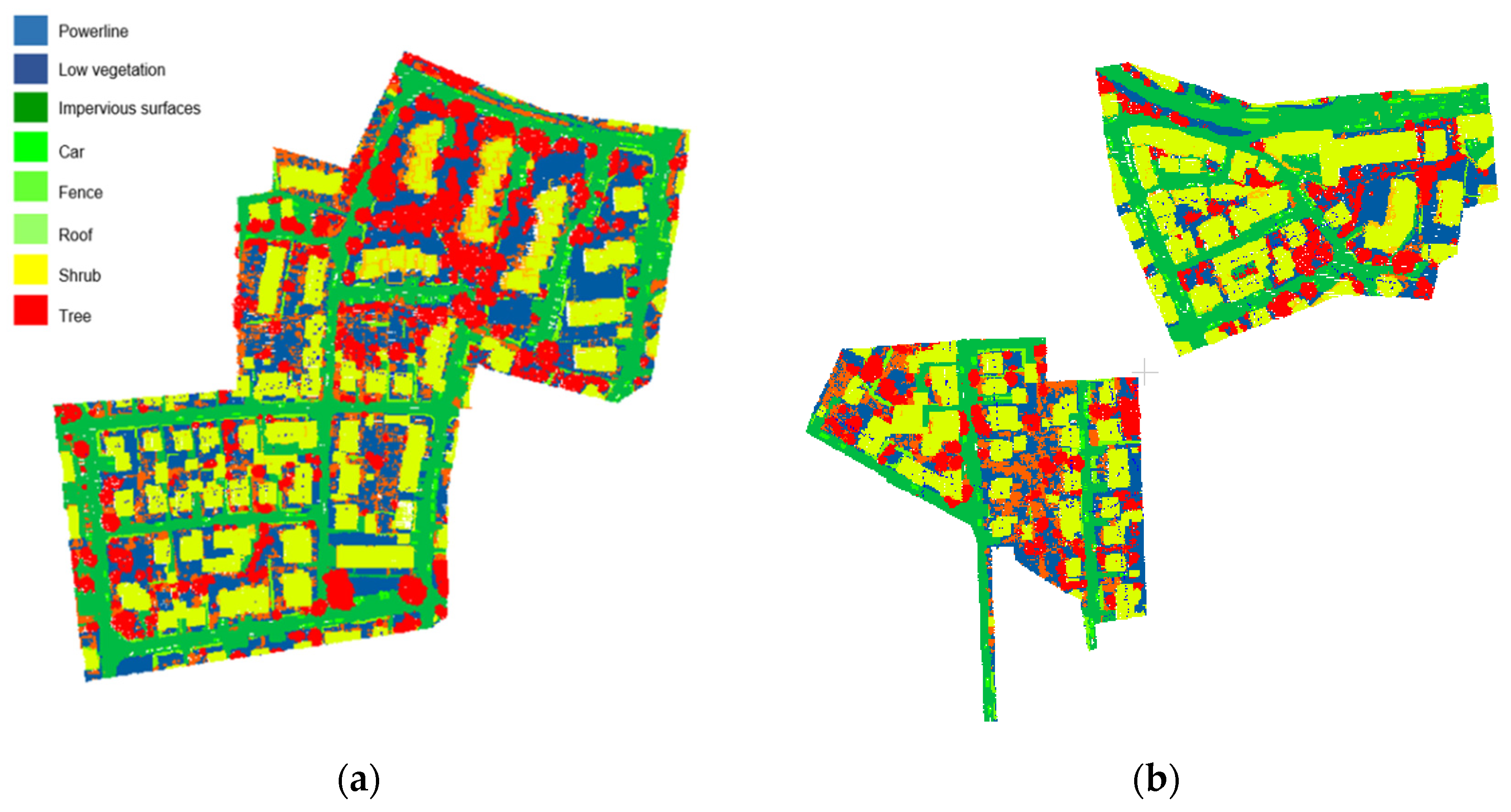
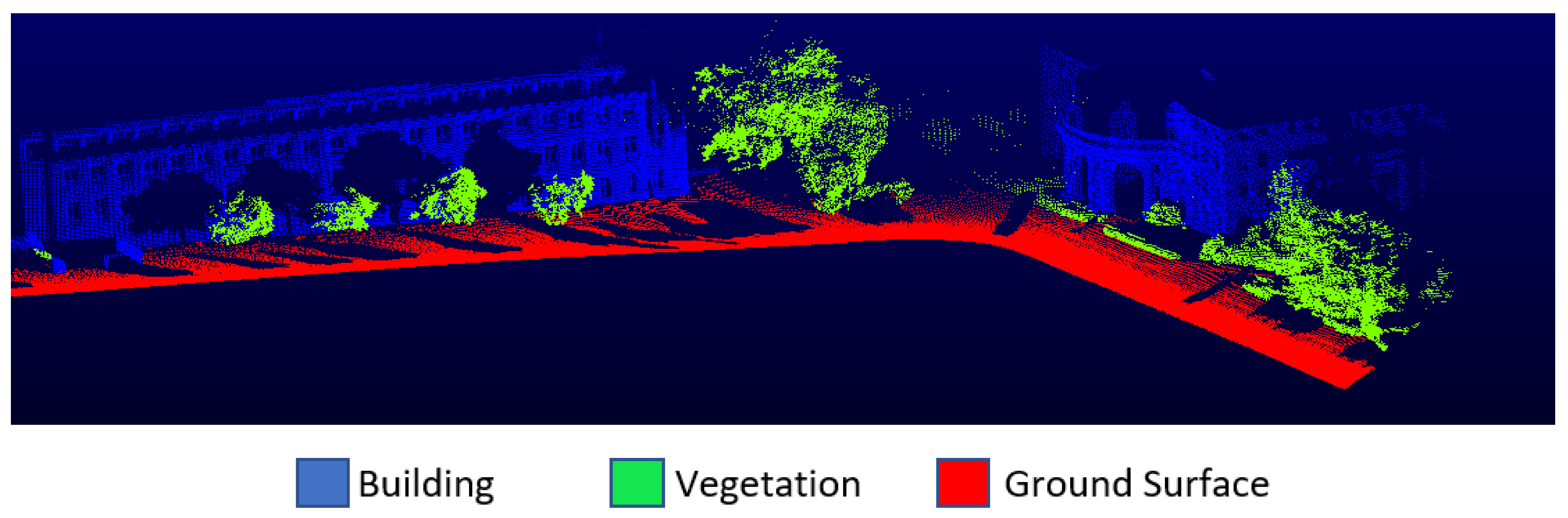
The Vaihingen dataset (
Figure 3) consisted of training that had 753,859 points and testing parts that had 411,722 points. The Vaihingen dataset included 9 classes, namely powerline, low vegetation, impervious surface, car, fence/hedge, roof, façade, shrub and tree. The classes were reduced into three classes to simulate this dataset to the Dublin dataset for an accurate comparison. Power line, car and fence/hedge classes were eliminated as they had few points. The ground surface class was created by combining low vegetation and impervious surface. Building class was formed by combining roof and façade. The vegetation class was created by combining tree and shrub.
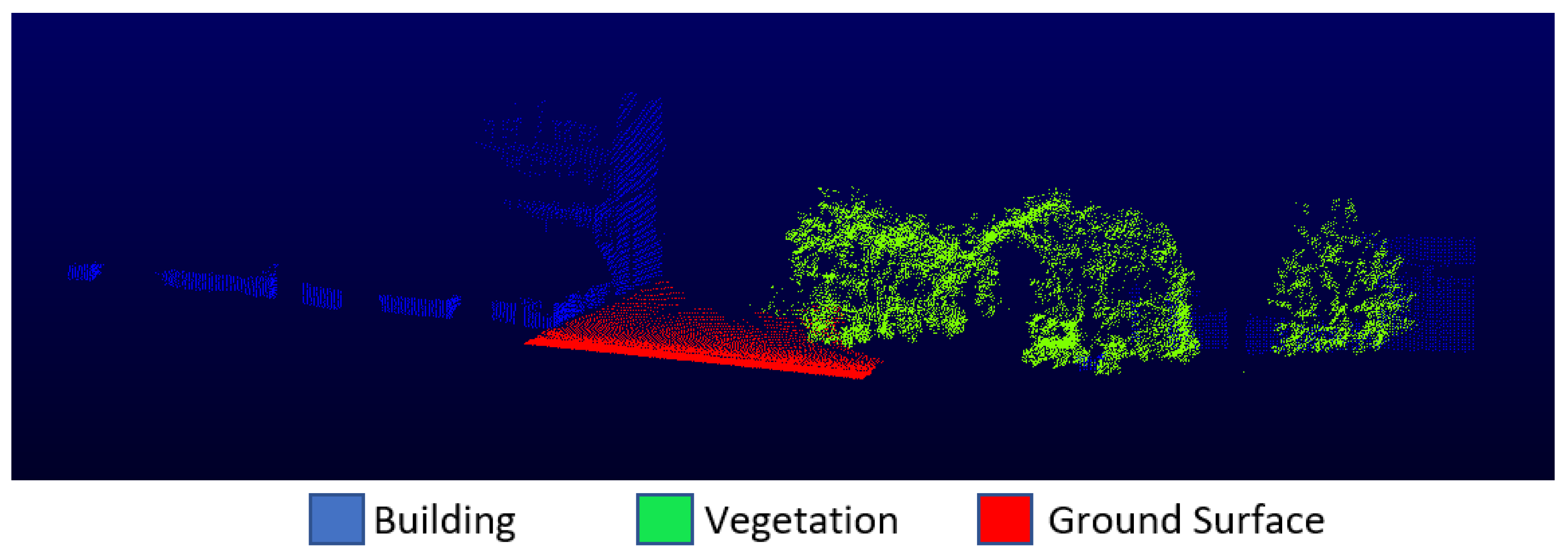
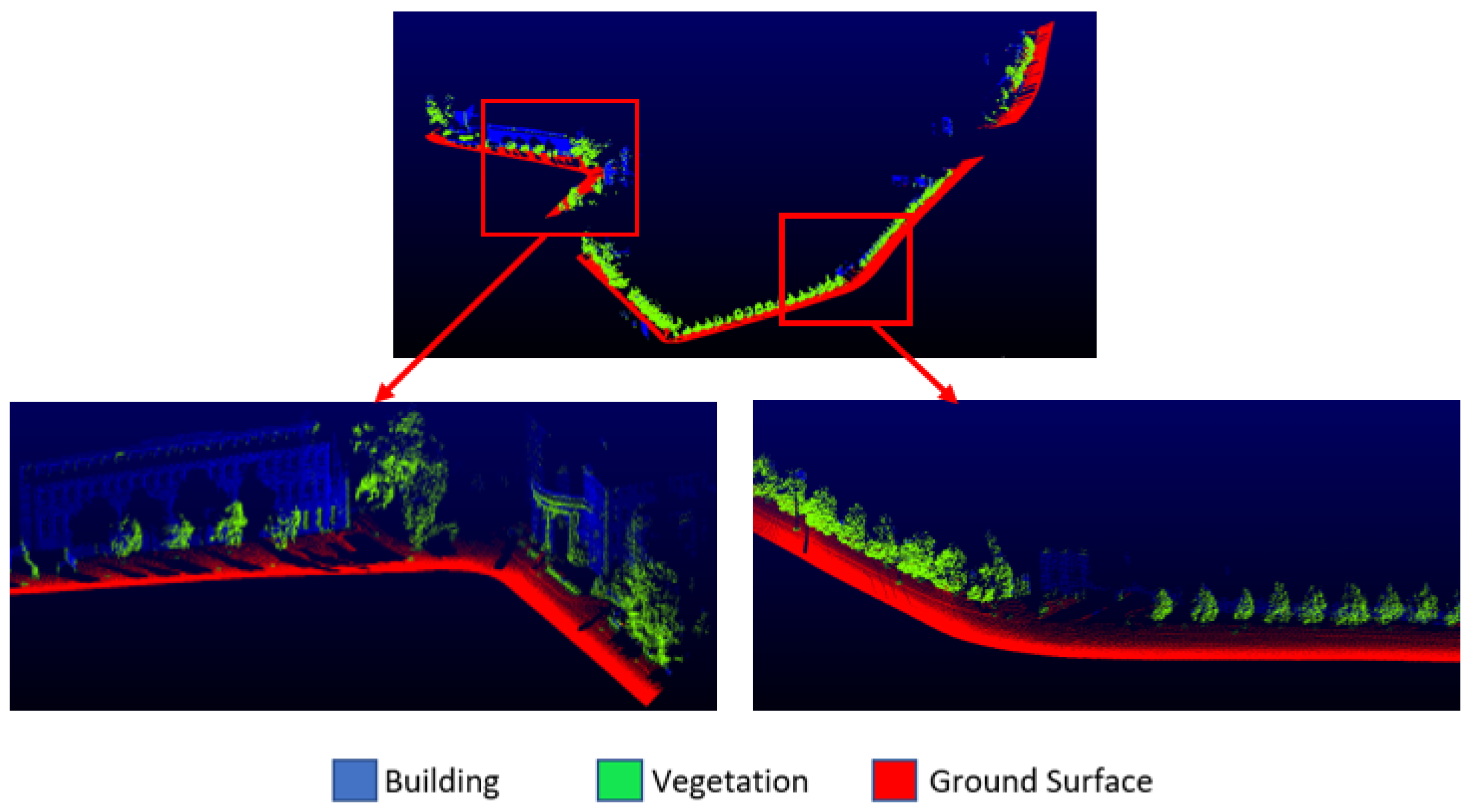
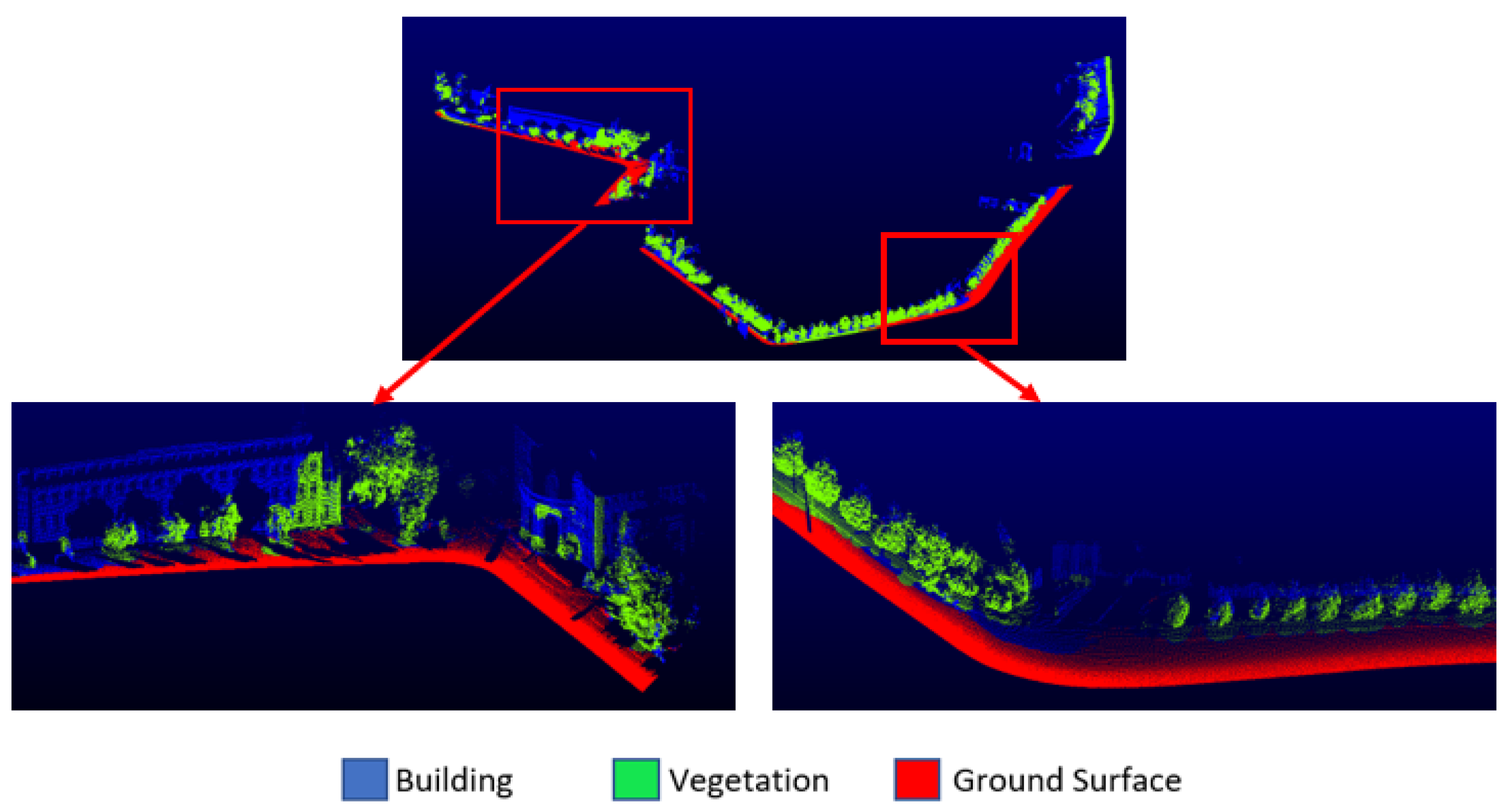
The Oakland dataset, one of the most used MLS datasets, was also selected for the application. This dataset was obtained with a mobile platform and covers the urban environment. The Oakland dataset consists of 36,932 training points, 91,579 validation points and 1.3 million testing points, which include 5 classes, namely ground, vegetation, façade, wire and pole/trunk. The wire and pole/trunk classes were removed, so they contain a few points. The façade class was renamed as building. Training (
Figure 4) and testing (
Figure 5) parts were used in the study. All datasets had ground truth. The distribution of the training and test data of the datasets are given in
Table 1.
The Dublin City and Vaihingen datasets had relabeled land-use types consisting of 3 classes; building, vegetation and ground surface. Firstly, support (S) areas of 0.5 m, 1 m, 1.5 m, 2 m and 3 m were created for each point. 13 geometric features were calculated in each support created. Geometric features were expressed as functions of the eigenvalues of the covariance matrix of the set of points located in a certain support area. Feature space was prepared for each point with the calculated geometric features and z coordinate values of the points. Thus, it was used as input data for machine learning algorithms.
3.2. Random Forest (RF)
RF [
17] is an improved version of bagging that creates a large collection of uncorrelated trees and then averages them. It is quite similar to boosting the performance of random forests in many problems and is easier to train and adjust [
18]. Each tree in the random forest gives a class estimate, and the top voted class becomes the model’s prediction. In the bagging algorithm, multiple bootstrap training data sets are created from the original training data set to train a classifier, and a training data set is assigned to each tree. There are two reasons to use bagging. First, the use of bagging appears to increase accuracy while using random features. Second, bagging can be used to give estimates of power and correlation as well as estimates of the generalized error (
PE*) of the combined tree community [
17].
Two parameters are required to generate a tree with the RF classifier. These parameters are the number of variables used in each node and the number of trees to develop to determine the best split. Boot samples are created from 2/3 of the training data set. The remaining 1/3 of the training data set, also called out-of-bag (OOB) data, is issued to test errors. The error obtained from this process is called the generalized error. Generalized error calculation is shown in Equation (1):
where
mg() refers to the margin function. Margin measures how much the average number of votes in (
X,
Y) for the correct class exceeds the average rating for any other class. The more reliably the classification can be performed, the larger the margin [
17].
3.3. Naïve Bayes (NB)
Classifiers work by computing one separator function for each class and assigning a sample to the class in which the function takes its largest value [
19]. For example, assume that a is a vector of attributes, as in typical classification practices. In the example, let
vjk be the value of the attribute
Aj,
P (
X) represents the probability of
X and
P (
Y|
X) the conditional probability of
X given
Y. Then, a possible set of separator functions can be expressed as Equation (2):
The classifier obtained using this set of discriminant functions and predicting the related probabilities in the training set is usually called the Naïve Bayes classifier [
20]. Naïve Bayes ‘classifier is a probabilistic classifier based on Bayes’ theorem. Its starting point is Bayes’ conditional probability theorem and it examines the probabilistic relationship between a particular data point x and class C [
21].
Although it has different types, it is the most widely used Gauss Naïve Bayes classifier. Gauss Naïve Bayes (GNB) applies classification by assuming the probability of the properties to be Gauss [
22]. The formulation is as Equation (4):
3.4. Multilayer Perceptron (MLP)
MLP is a sensor with a single weight layer that can only operate on linear functions of the input. It cannot give successful results on nonlinear functions. Multi-layer perceptron can solve such nonlinear problems if used for classification [
23]. Multi-layer Sensor is a supervised learning algorithm that learns a function by training on a dataset. MLP can learn a nonlinear function approach for classification or regression. There may be one or more nonlinear layers, called hidden layers, between the input and output layer. Therefore, it is different from logistic regression [
24]. In MLP, there are transitions between layers called forward and backward propagation. In the forward propagation phase, the output of the network and the error value are calculated. In the backpropagation phase, the connection weight values between the layers are updated to minimize the calculated error value.
The input layer is fed with the input x value. The “activation” propagates in the forward direction and
zh values are calculated in the hidden layers. Each hidden layer unit is a detector on its own and applies the nonlinear sigmoid function to its weighted sum:
To calculate
yi values in the output layer, the sensors in this section use the values calculated in hidden layers as input values [
23].
3.5. Logistic Regression
In logistic regression, the probability that the output variable belongs to the appropriate class is calculated [
25]. Logistic regression [
26] establishes a linear transformation between the output variable and input variables. However, a linear transformation is performed between input variables and probabilities of the output categorical variable, instead of between the output and the input variables. Input variables need not be continuous, normally distributed or independent. The result is the probability of an observation for a category, not a class. The mathematical model for the logistic regression classifier can be expressed as:
where
Y is the output variable,
αi and
βj are the coefficients of the model, and x
1, x
2, …, x
p are the covariates. The basic mathematical concept that defines logistic regression is logit, which can be defined as the natural logarithm of a probability ratio. Each observation is assigned to the class of maximum probability:
In general, logistic regression is well suited for explaining and testing hypotheses about relationships between a categorical output variable and one or more categorical variables [
27].
3.6. Linear Discriminant Analysis (LDA)
Linear Discriminant Analysis (LDA) [
28] is the oldest classifier currently in use, is a linear transformation that calculates the directions of the axis that best distinguishes multiple classes. If we define this direction as w, the data is projected onto the defined w direction. Thus, the sample data of the two classes are tried to be separated as much as possible.
z is the projection of data (
x) onto
w. After the projection, to separate the classes well, it is aimed to keep the average of the samples belonging to the classes as far from each other as possible and to distribute the class samples to as small an area as possible. In LDA, it is aimed to have a maximum ratio of within-class (
Si) and between-class (
SB) scatter matrices (R =
Si/
SB).
The algorithm tries to assign elements to each class, maximizing R [
23]. The solution is the largest eigenvectors of
, where S
w is the sum of the within-class scatter matrix. LDA assumes that attributes (input or explanatory variables) are continuous and normally distributed, while the dependent variable, which is the output value (such as a class), is categorical [
15].
3.7. Decision Tree (DT)
Decision tree (DT) is one of the algorithms that divides the input space into parts and calculates parameters for each part. Decision tree is a non-parametric classification and regression algorithm. Each node in the decision tree is associated with a part, and nodes divide each part into sub-parts. If the size of the decision tree is not predetermined, it can be considered as an algorithm that is non-parametric [
29].
Besides being easy to apply, decision tree has some disadvantages. It can create a complex tree on the data. Decision trees can be unstable because small changes in data can result in producing a completely different tree. However, it is still a useful algorithm due to computational limitations.
3.8. Support Vector Machines (SVM)
Support Vector Machines (SVM) [
30] is a supervised machine learning algorithm used for both classification and regression. The aim of the support vector machine algorithm is to find a hyperplane in an N-dimensional space that has the maximum distance between data points of both classes and classifies the data points separately. The optimal hyperplane can be obtained by using Equation (12). For a given set of a sample
:
where
is an N-dimensional vector and
is a scalar, and they are used to define the hyperplane. There are two hyperplanes that separate the samples and are not points between them, to separate samples in a dataset linearly [
31]. In this study, a linear SVM algorithm optimized with Stochastic Gradient Descent (SGD) is used. SGD is one of the most popular optimization algorithms used in machine learning in large data sets due to the ability to efficiently optimize the entire training set depending on the number of data epochs [
32]. It aims to approximate the gradient of the objective function using small randomly selected subsets of training examples. SGD chooses a point in each iteration or a set of points based on batch size to reduce a large processing load, rather than using all the data for learning. Depending on the amount of data in SGD, a balance is struck between the accuracy of the weight update and the time it takes to perform an update. In one iteration, the weights are updated according to each random point or set of points selected. Thus, the gradient of the sample i selected in t iteration ∇E (W
t, x
i, y
i) is calculated instead of the true gradient (∇E) [
33].
3.9. K-Nearest Neighbor (KNN)
K-nearest neighbor (KNN)-based classification is a type of sample-based learning or non-generalized learning. It does not attempt to create a general internal model [
34]. The nonparametric k-nearest neighbor algorithm is not constrained by a fixed number of parameters. Since KNN does not contain parameters, it generates and applies a function dependent on training data. For each data in an input data set X, k’s closest neighbors are found. Neighboring points are weighted in inverse proportion to their distance from the query point. Afterward, the most common class in the neighborhood is assigned as the class x data [
23].
3.10. Extraction of Geometric Features
Geometric properties are useful for explaining the local geometry of points. These geometric features are nowadays widely applied in LiDAR data processing. It is aimed to improve the accuracy values by extracting these geometric features in multiple scales rather than on a single scale. Geometric features are calculated by the eigenvalues (λ
1, λ
2, λ
3) of the eigenvectors (v
1, v
2, v
3) derived from the covariance matrix of any point p of the point cloud:
where
is the centroid of the support S. Many values are calculated using eigenvalues: the sum of eigenvalues, omnivariance, eigenentropy, anisotropy, planarity, linearity, surface variation, sphericity and verticality. Calculated values are normalized. Since the datasets used contained only geometric information (3D coordinates), only geometric features were used in the study (
Table 2).
The relevant geometric properties of any point in the 3D point cloud were based on the support of the point. Support selection is an important issue as the distinctiveness of the geometric features depends on the relevant support considered for feature extraction [
9].
3.11. Experiment
In the first step of the experiment, 13 different feature geometric features were calculated for each data set. Geometric properties were obtained by using spheres with radii of 0.5 m, 1 m, 1.5 m, 2 m and 3 mto apply the classification at different scales.
R0.5; represents the support calculated with a radius of 0.5 m.
R1; represents the support calculated with a radius of 1 m.
R1.5; represents the support calculated with a radius of 1.5 m.
R2; represents the support calculated with a radius of 2 m.
R3; represents the support calculated with a radius of 3 m.
First, the classes of the data were arranged and were reformatted according to algorithms. In the Vaihingen dataset, since there were few points in the power line, car and fence/hedge classes, they were deleted from the dataset. However, wire and pole/trunk classes also had fewer points in the Oakland3D dataset, so they were removed from the dataset.
In the study, point clouds were classified using eight different machine-learning algorithms: LDA, RF, GNB, LR, MLP, DT, SVM and KNN. Scikit-learn, a machine learning library prepared for the Python programming language, was used to implement the methods. The optimized parameters for all methods were determined and were unchanged during the study. In the study, a computer was used with I7 7700HQ 2.8GHZ, 16GB RAM, GTX1050Tİ 4GB graphics card.
Four metrics were used: precision, recall, F1 score for each class and overall accuracy for evaluating of the methods. Precision measures the proportion of points classified as positives (Equation (14)). Recall measures the proportion of positives that are true positives (Equation (15)) [
23].
F1 score is a function of precision and recall (Equation (16)) [
35]. Overall accuracy measures the proportion of points correctly classified. Accuracy metrics are obtained using confusion matrices generated as a result of classification. All accuracy analyzes were carried out in the Python programming language.
True positive (
TP) is the number of points that have the same label in predicted and ground truth. False positive (
FP) refers to the number of points that are predicted positive but their actual label is negative. False negative (
FN) refers to the number of points that are predicted negative and their actual label is positive [
23].
4. Results
The proposed methodology was applied to the three different areas selected from two different datasets. It was aimed to determine the most suitable support radius for each method. The classification process was repeated in the same way for each case. Points that did not have sufficient neighbor points for geometric properties were eliminated from the point cloud.
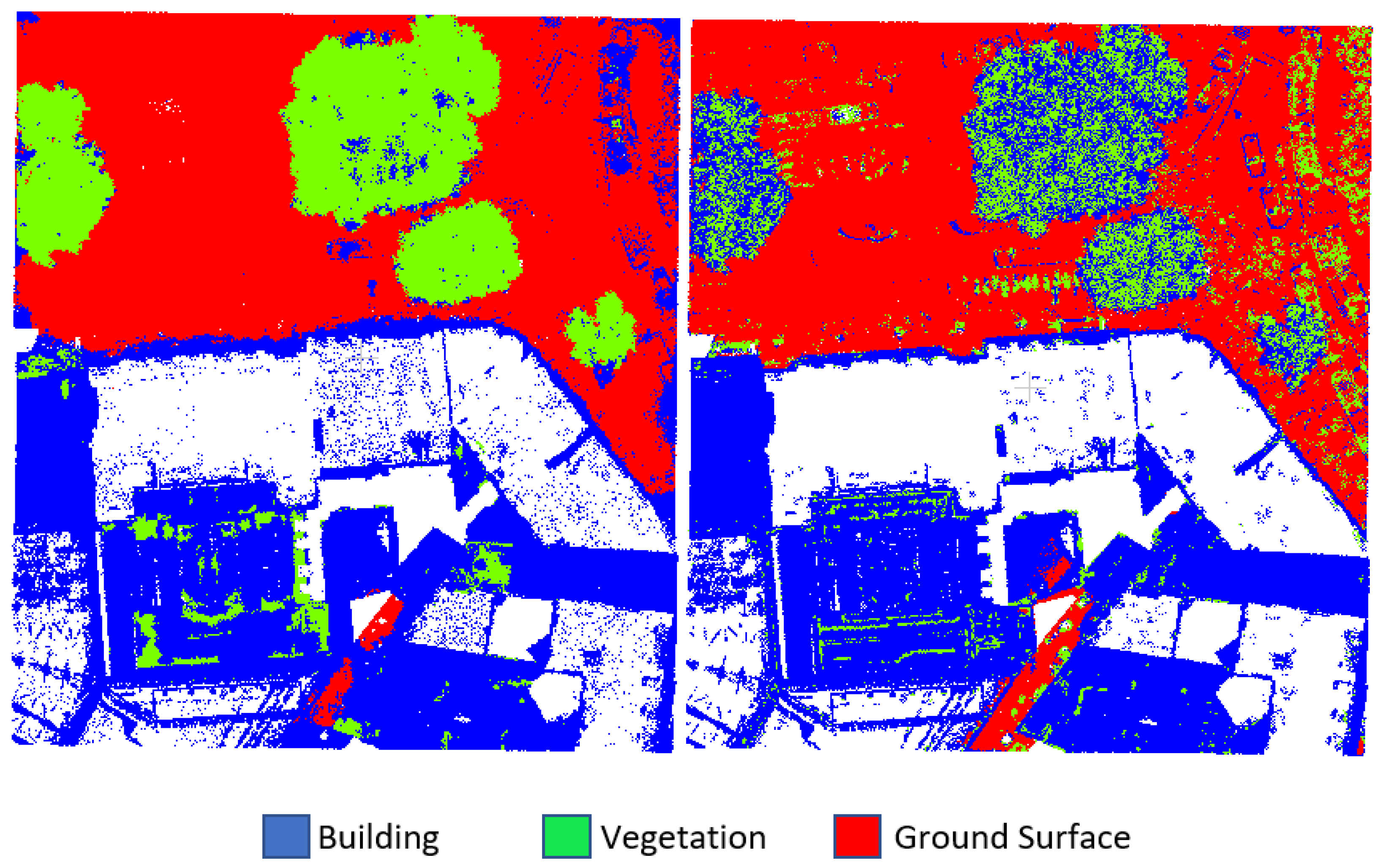
According to results in Dublin City Area 1, the highest overall accuracy in algorithms other than GNB, KNN and DT was obtained when using a support radius R
3 (
Table 3). The RF method had the highest accuracy of 93.12% (
Figure 6). The second-highest accuracy belonged to the MLP method with an overall accuracy of 93.07% with R3. The SVM method has the lowest overall accuracy at 83.27% with R
0.5 in Dublin City Area 1 (
Figure 6). According to the results in different scales, the lowest accuracies were obtained in cases where the support radius of 0.5 m was used. The reason for determining a maximum radius of 3 m is that the calculation load and the time spent increase as the radius increases for the calculation of geometric properties.
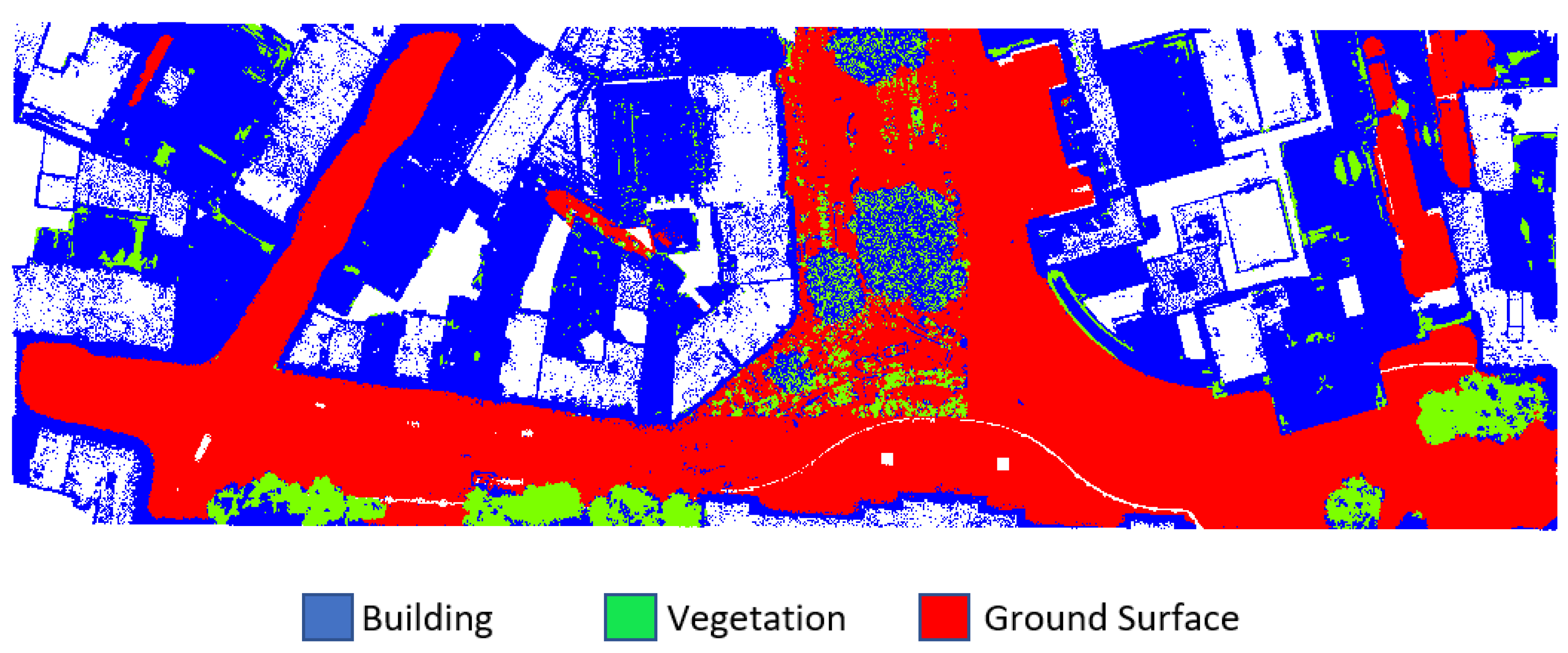
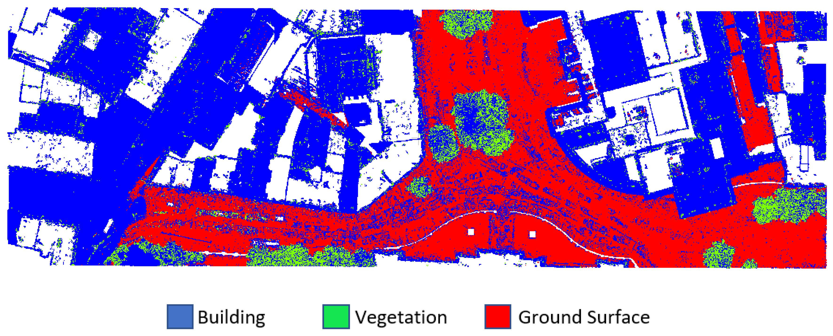
In Dublin City Area 2, 6 out of 8 methods presented the best results when using a support radius of 3 m. The GNB and KNN methods achieved the highest overall accuracy using supports R
05 and R
1.5, respectively. In the Dublin dataset, GNB and KNN methods were successful with a smaller support radius. MLP and SVM had better overall accuracy with 92.78% (
Figure 7) and 91.59%, respectively. The least accurate method was the LDA method with 84.79% overall accuracy (
Figure 8). The overall accuracy of the all methods in Dublin City Area 2 was represented in
Table 4.
The Vaihingen dataset covered a comparatively smaller area than Dublin City Area 1 and Dublin City Area 2. Geometric features could not be calculated since most of the points in the support of R
05 did not have sufficient neighboring points. For this reason, R
0.5 support was not evaluated for the Vaihingen dataset. All methods except KNN had their best results in the R
15 support. Unlike the Dublin City dataset, the accuracy of all methods decreased with the larger supports (R
2 and R
3) in the Vaihingen data. The two most accurate methods, SVM and MLP, had an overall accuracy of 79.71% and 77.68%, respectively. RF had the lowest accuracy with 68.26% accuracy (
Figure 9). The overall accuracy of the all methods in the Vaihingen dataset is represented in
Table 5.
The Oakland3D dataset had a similar size to Vaihingen. The highest accuracy values were obtained in R
1 and R
1.5 supports for all methods except SVM and KNN methods. The highest accuracy was achieved as 97.30% with the LDA method in R
1 support (
Figure 10). The LDA and RF methods provided sufficient accuracy for all support sizes. Although the accuracy values decreased slightly as the support size increased, accuracy of around 90% was obtained. The DT method has low accuracy in support sizes except for R
1.5. 94.12% general accuracy was obtained with the DT method in R
1.5 support. The method with the lowest accuracy of 66.78% is the GNB method in R
3 support (
Figure 11). General accuracy values of the Oakland version are presented in
Table 6.
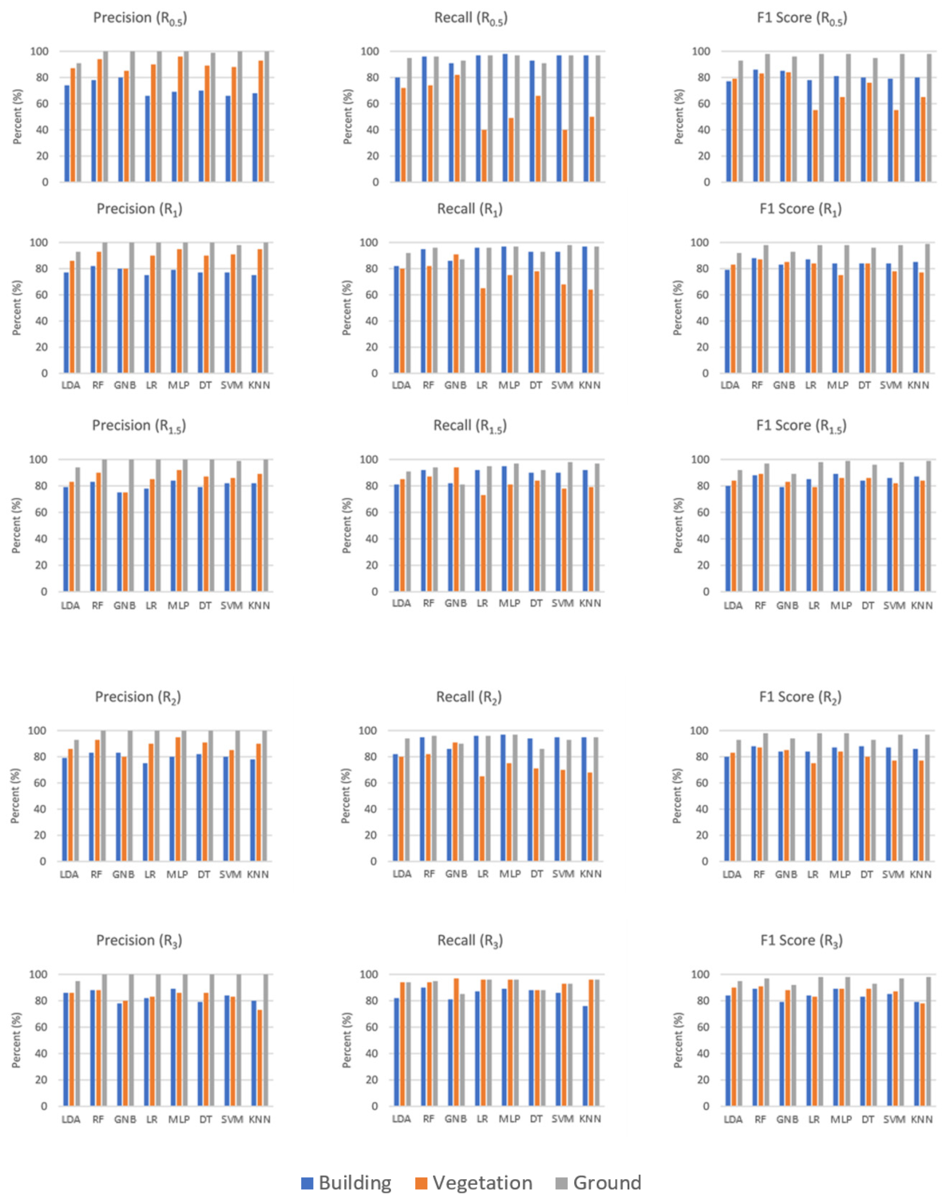
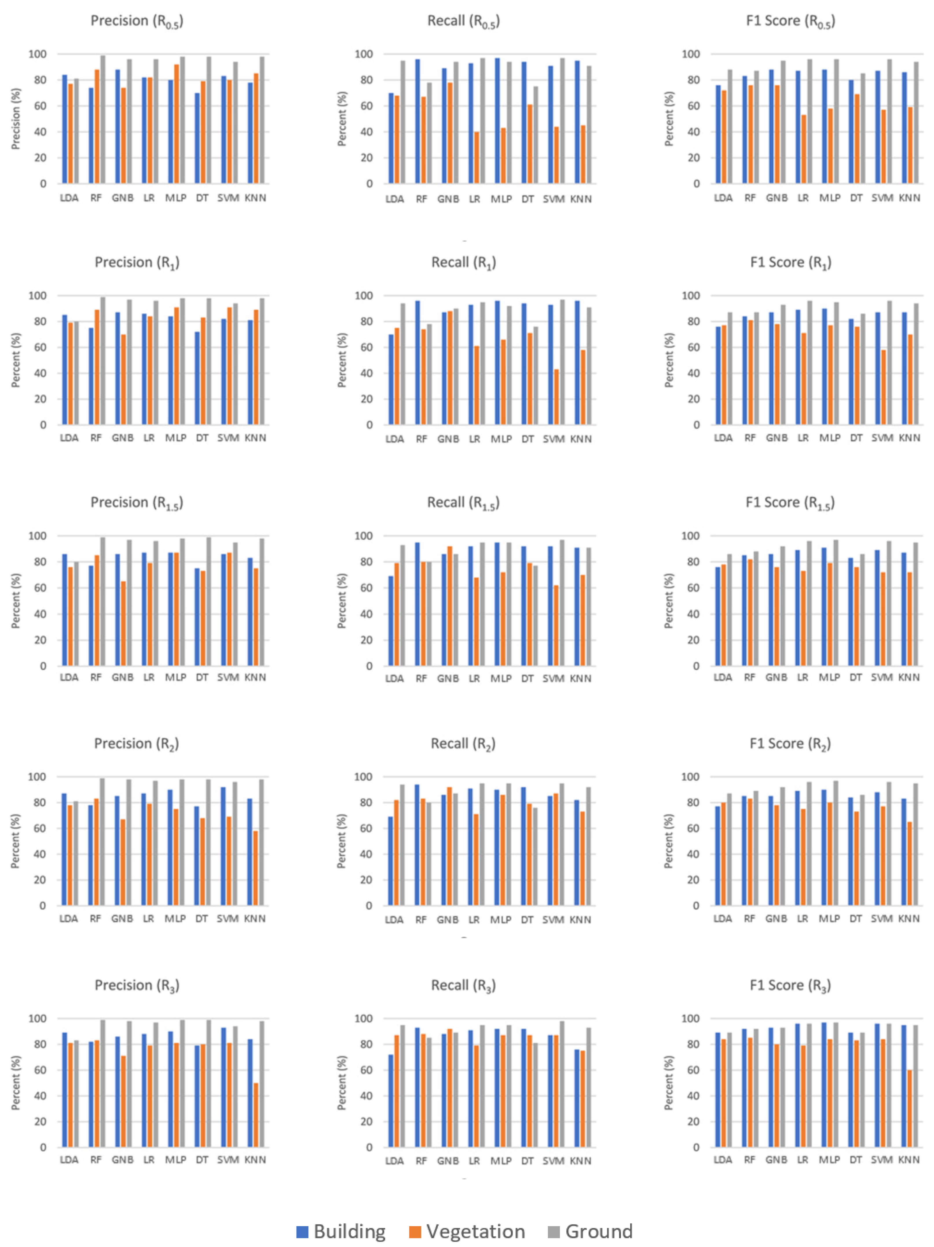
Precision, recall and F1 score values of each class were also calculated. It was found that in Dublin City Area 1, all classes were detected better as the radius increased. Considering the F1 score, the RF method was the best method for the building class. RF was slightly affected by radius change for the building class. It had an F1 score of 88% for R
0.5 and 89% for R
3. The KNN method was the most unsuccessful method for the building class. The vegetation class had lower accuracy values in a small support radius. The highest F1 score for vegetation was obtained for RF (91%) in the R
3 support. It has been determined that the KNN method was insufficient for the vegetation class regardless of the support size. KNN generally had a high precision value and low recall value. The opposite was true in the R
3 support. It had a low recall value in the support of R
0.5 in all methods. In other words, although the methods correctly detected the majority of vegetation class in small supports, most of the points labeled as vegetation belonged to different classes. The ground surface class had been extracted with approximately 100% precision, recall and F1 score in all cases (
Figure 12).
In Dublin City Area 2, there were some differences from Dublin City Area 1. While all values increased rapidly in support radius greater than R
0.5 in Area 1, the values of metrics at a small radius in Area 2 did not increase in the same way. High metric values were obtained in the support of R
3 for almost all methods. Although precision was not affected by the radius change, recall and F1 score had low values in the support of R
0.5. MLP and LR (in R
3 support), the best methods for building class extraction, had 97% and 96% F1 scores, respectively. The method with the lowest F1 score was the LDA method with 89% (in R
3 support). Vegetation class was detected with lower success in all supports than other classes. For the vegetation class, RF was the most successful method in terms of F1 score (86% for R
3). KNN was quite insufficient for extraction of vegetation. The highest F1 score was obtained with 72% in R
1.5 support. Although the ground surface class did not have values close to 100% in Area 2 as in Area 1, because the test data was larger, precision, recall and F1 scores were generally obtained above 90% for all methods (
Figure 13).
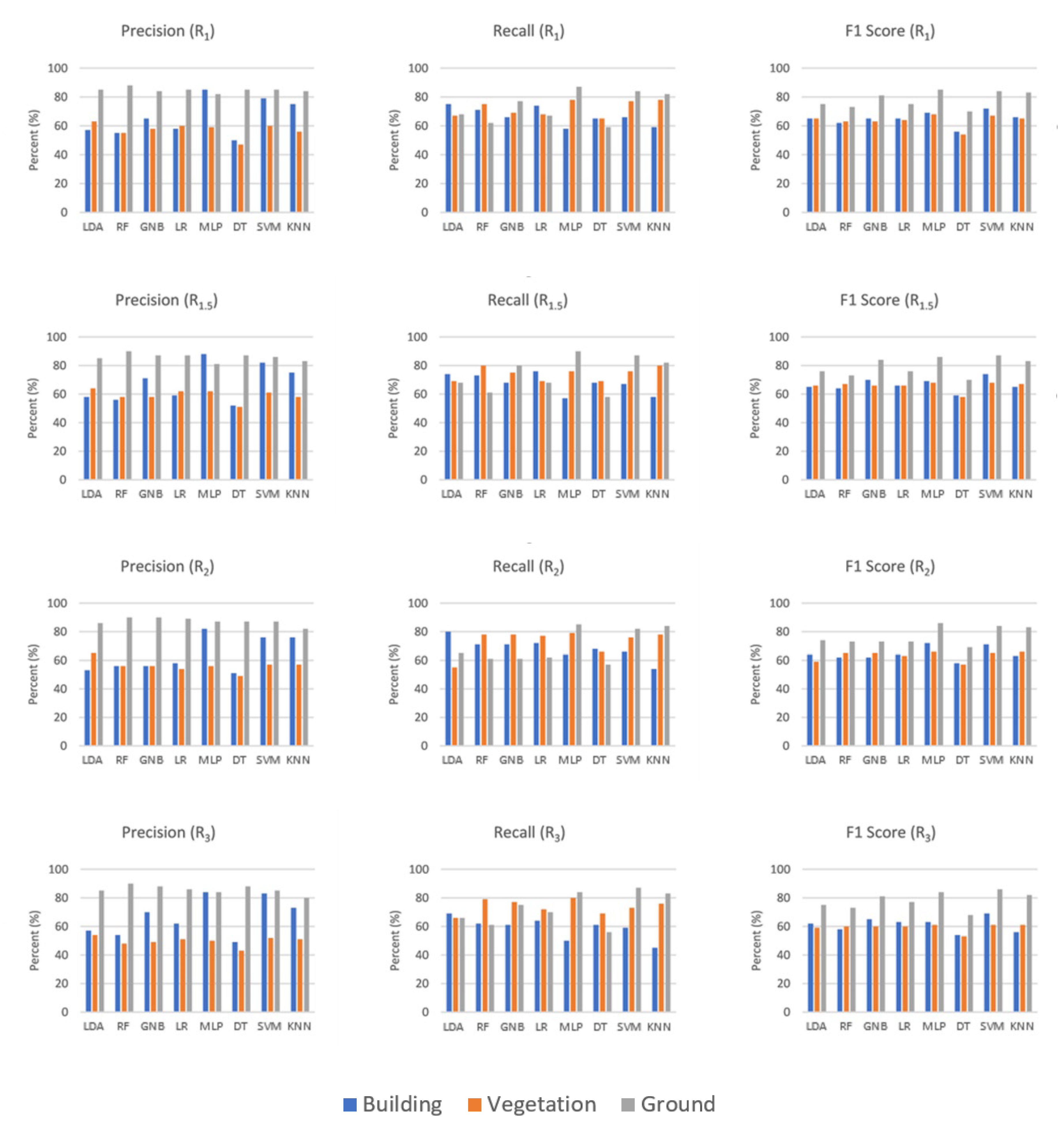
In the Vaihingen dataset, lower metrics were obtained for all methods compared to the Dublin City dataset. In the Vaihingen dataset, recall values were higher than precision values. In other words, although most of the labeled points were labeled correctly, they could not find the points belonging to that class with the same success. For the building class, the SVM method had the highest F1 score value (74% in R
1.5 support), while the lowest F1 score value was obtained in the DT method (54% in R
3 support). Similar results to the building class were obtained for the vegetation class. MLP (68% in R
1.5 support) and SVM (68% in R
1.5 support) have the highest F1 score value. The lowest F1 score (53% in R
3 support) was obtained by the DT method. The methods again extracted the ground surface class better than the other classes. For the ground surface class, SVM (87% F1 score in R
1.5 support) was the best method while the worst method was DT (68% F1 score in R
3 support). When using large supports (R
2 and R
3) in the Vaihingen dataset, a decrease was observed in all metrics (
Figure 14).
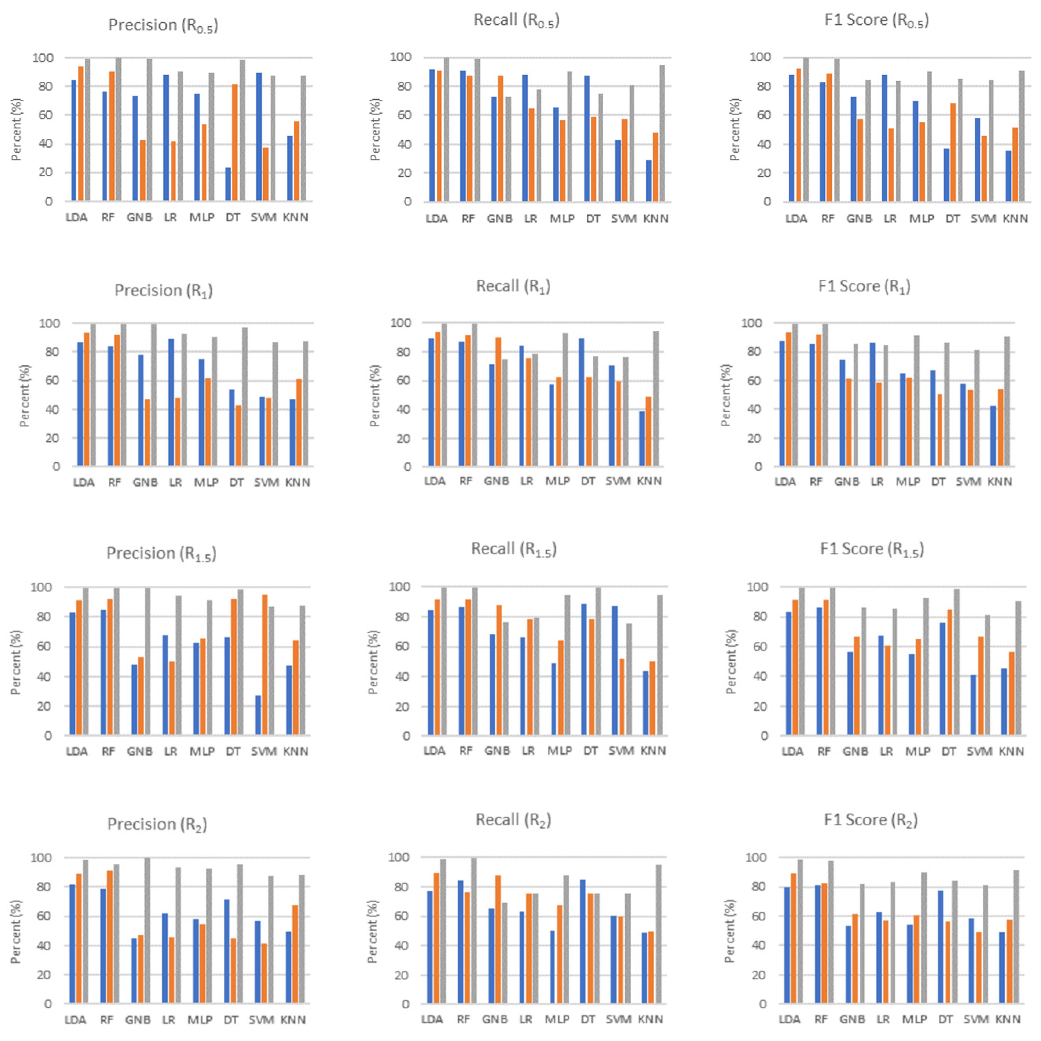
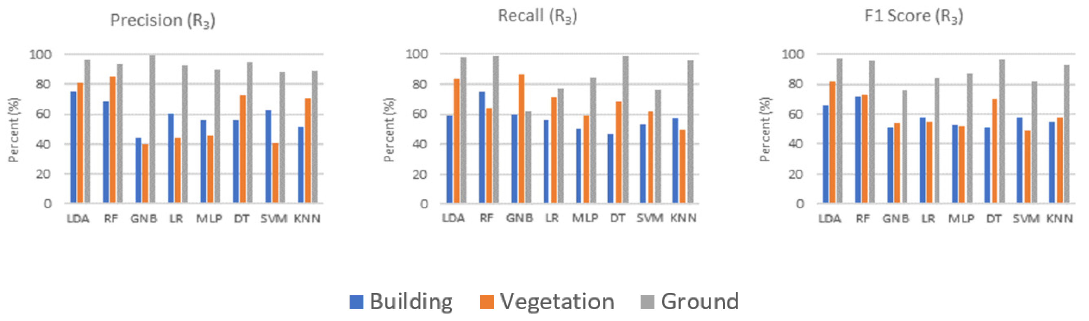
In the Oakland3D dataset, it was determined that better results were obtained in R
1 and R
1.5 supports. As with the Vaihingen dataset, recall values were higher than precision values at all scales. Especially in R
2 and R
3 supports, a decrease was observed in all accuracy metrics. Similar to other datasets, insufficient accuracy was obtained in R
05 support. For building class, while the highest F1 score was obtained with LDA (88% in R
1 support), the lowest F1 score was obtained with KNN (36% in R
0.5 support). For vegetation class, LDA has the highest F1 score (94% in R
1 support), SVM has the lowest F1 score (45% in R
0.5). The ground surface class was extracted with higher accuracy compared to other classes. When RF has the highest F1 score (%99 in R
1 support), GNB has the lowest F1 score (76% in R
3). The precision, recall and F1 scores of the Oakland3D dataset were shown in
Figure 15.
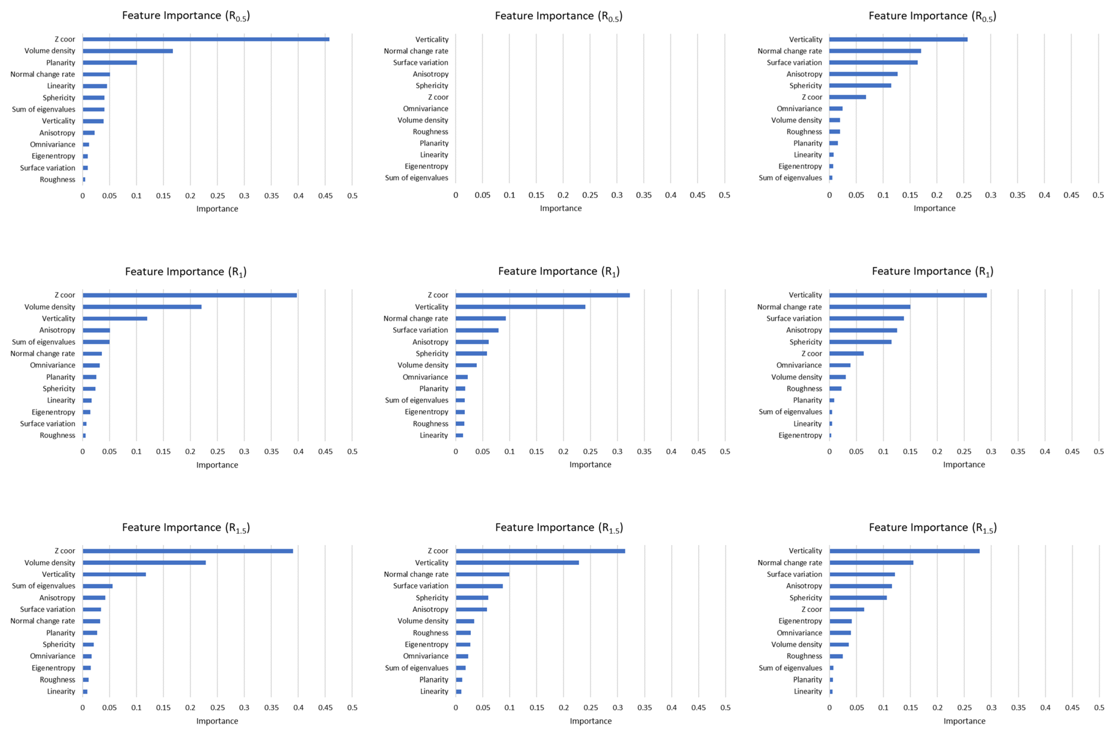
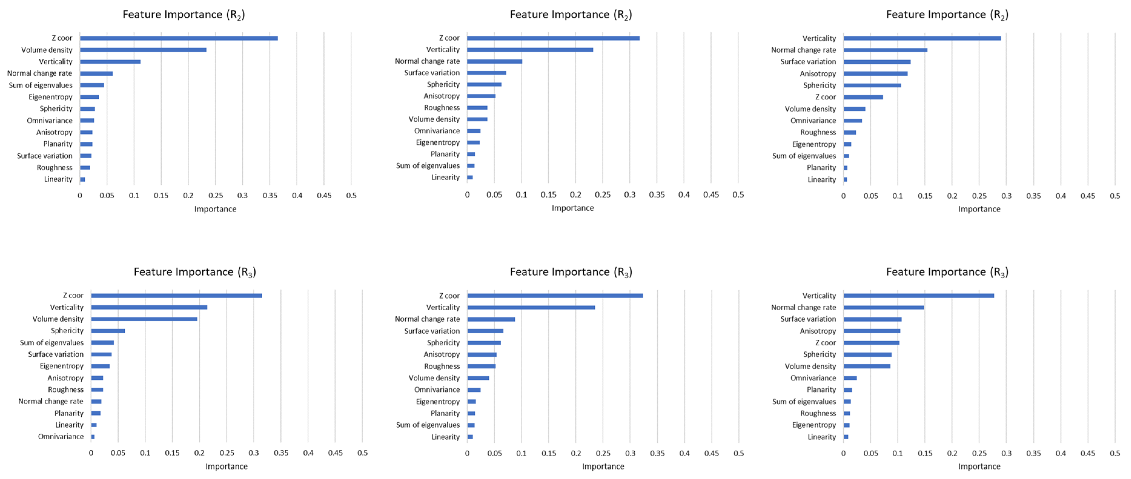
Geometric features affected the accuracy at different rates. This situation was defined as feature importance. Some methods calculate the feature importance value. RF is a method to obtain an ordered list of them. The most important feature in both datasets was the Z coordinates of the points. Other important features for the Dublin City dataset were verticality and volume density. The least important feature was linearity. The roughness feature was also of low importance except for the R
3 support. In the Vaihingen dataset, verticality was the second most important feature. While the least important feature was Linearity, the importance of roughness increased as the support radius grew. Since most of the values were obtained as NaN, no evaluation was made for R
0.5 in the Vaihingen dataset. Feature importance values calculated for each study area were presented in
Figure 16.
5. Discussion
The results of the study allow general inferences to be made regarding the selection of some optimum parameters for point cloud classification. Determining the optimum support size is one of the most important factors affecting the classification accuracy. Considering the overall accuracy metrics, it was determined that the optimum support size may not be the same for different classes (
Figure 12,
Figure 13,
Figure 14 and
Figure 15). Furthermore, the idea that the optimum support size depends on the respective point density is meaningful and is consistent with previous studies [
9]. In both test sites of the Dublin City dataset which had very high point density, generally, the highest accuracy results were obtained at the R
3 scale, a large support size (
Table 3 and
Table 4). In the Vaihingen and Oakland3D datasets that had less density, generally the highest accuracy results were obtained in R
1 and R
1.5 support sizes (
Table 5 and
Table 6). Accordingly, it is appropriate to choose a larger support size in denser point clouds and choose a smaller support size in low-density point clouds. Additionally, it has been shown that the optimum support length can vary from one algorithm to another. For classification methods, DT, a rule-based method, generally did not give good results compared to other methods. Although higher classification accuracies are obtained with the instance-based KNN method, it has a long test time. It has been determined that the classification accuracy of LDA, GNB and LR (probabilistic methods), RF (ensemble method), SVM and MLP (neural-network-based method) methods are improved. However, the MLP method has a disadvantage with its long training time. Even though LR, GNB and SVM could compete with other methods in the Dublin City and Vaihingen datasets, they were insufficient in the Oakland3D dataset. The LDA and RF methods also had high classification accuracy in the Dublin City and Oakland 3D datasets, but showed lower performance in the Vaihingen dataset than other classifiers. It was understood that choosing the appropriate classifier depends on the scale and data set. The findings of this study were compared with previous studies with the same datasets. Since the Dublin City dataset is a new dataset, there is no study in the literature comparable to this study. Comparative results for the Vaihingen and Oakland3D datasets are presented in
Table 7 and
Table 8.
Algorithms were also evaluated in terms of test and train time. There are many factors, such as the size of the dataset, the parameters selected and the hardware used, which affect the time. Therefore, although the processing times of the algorithms were specific to this study, they provided important information as they were evaluated under the same conditions.
As expected, algorithms needed more tests and train time for the larger dataset. GNB had the shortest training time, while MLP training time was the longest. MLP as a neural network, having hidden layers, took time for training. According to test times, DT was the fastest algorithm while KNN was the slowest algorithm. KNN was slow because it determined the closest neighbor points for each point individually. In all algorithms except KNN, the training time was longer than the test time. The duration of the algorithms is presented separately for each dataset in
Table 9.


