Prediction of Potential and Actual Evapotranspiration Fluxes Using Six Meteorological Data-Based Approaches for a Range of Climate and Land Cover Types

Abstract

Evapotranspiration is the major component of the water cycle, so a correct estimate of this variable is fundamental. The purpose of the present research is to assess the monthly scale accuracy of six meteorological data-based models in the prediction of evapotranspiration (ET) losses by comparing the modelled fluxes with the observed ones from eight sites equipped with eddy covariance stations which differ in terms of vegetation and climate type. Three potential ET methods (Penman-Monteith, Priestley-Taylor, and Blaney-Criddle models) and three actual ET models (the Advection-Aridity, the Granger and Gray, and the Antecedent Precipitation Index method) have been proposed. The findings show that the models performances differ from site to site and they depend on the vegetation and climate characteristics. Indeed, they show a wide range of error values ranging from 0.18 to 2.78. It has been not possible to identify a single model able to outperform the others in each biome, but in general, the Advection-Aridity approach seems to be the most accurate, especially when the model calibration in not carried out. It returns very low error values close to 0.38. When the calibration procedure is performed, the most accurate model is the Granger and Gray approach with minimum error of 0.13 but, at the same time, it is the most impacted by this process, and therefore, in a context of data scarcity, it results the less recommended for ET prediction. The performances of the investigated ET approaches have been furthermore tested in case of lack of measured data of soil heat fluxes and net radiation considering using empirical relationships based on meteorological data to derive these variables. Results show that, the use of empirical formulas to derive ET estimates increases the errors up to 200% with the consequent loss of model accuracy.

1. Introduction

Evapotranspiration (ET) is the major component of the water cycle [1]. It is fundamental in many different applied hydrology studies [2,3], hence its incorrect assessments impact the hydrological soil–water balance [4]. Eddy covariance (EC) stations are considered among the most reliable systems for determining the ET losses but there are limitations in their use. The limitations come from the high costs of installation and maintenance, in addition, long-term ET measurements are complex to obtain and even if observational data exist, algorithms for data pre-processing are time-consuming [5]. Furthermore, flux towers coverage at the global scale is evidently quite inhomogeneous and quite scarce in some areas of the world. For all these reasons, in time, many scholars have proposed different models for the prediction of actual (AET) and potential (PET) ET. Among a large number of models, the conventional meteorological data-based approaches, though could appear old fashioned, are still nowadays preferred. The reason is the simplicity of computation and in the large availability of meteorological data required for the simulation [6,7]. This aspect is essential especially in rural water basin contexts where the lack of data represents the major challenge in evapotranspiration water losses assessment [8,9].

Among the meteorological data-based approaches for PET prediction, radiation-based, temperature-based, and combination-based models can be listed [10,11]. Priestley and Taylor [12], Turc [13] and Abtew [14] models are among the most commonly used radiation-based methods. The category of the temperature-based models includes methods like Hargreaves, Thornthwaite, Blaney- Criddle, and Linacre approaches [15,16,17,18]. Penman-Monteith model [19] is one of the most popular [20] approach within the class of combination-based models. With respect to AET, one of the most relevant method among the meteorological data-based models is the Antecedent Precipitation Index (API) approach [21,22,23,24]. Complementary approaches are another class of data-based methods used for the prediction of AET. They gained widespread application under different climate conditions and land cover surfaces [8,25]. A number of different techniques based on the complementary relationship (CR) have been developed, among which the Advection-Aridity (AA) model [26,27,28], the Granger and Gray (GG) model [29,30], the CRAE model [31], and the modified Advection-Aridity (MAA) model [32]. Given the existence of alternative methods, it appears fundamental to select the most appropriate approach for the modeling process of ET fluxes so, in time, many scholars have carried out researches with the aim of comparing predictions from PET and AET routines with values of evapotranspiration losses measured from EC stations and from lysimeters [33,34,35,36,37]. The findings of these comparative researches did not allow identifying a single model that outperforms the others for a particular biome. In particular, [38] compared several PET models only for a single climate condition which refers to Poland and lies between a snowy climate and a warm temperate one, in addition, no mention has been done to the land cover of the selected stations. [39] tested six PET approaches for a single land cover dominated by forest and only for the warm humid climate which characterizes the south-eastern United States finding out that Priestley-Taylor performs better than the other PET formulas. Similarly, [40] tested the performances of six ET models only for the humid climatic condition in the western region of Fukuoka City and for a crop area and Thornthwaite model resulted the most accurate approach.

Only few authors tested ET models in different climates and land covers. [37] considered different climatic regimes across the world and several vegetation types including grassland, cropland, savannas, and forest but this study mainly focused on PET models like PM and PP approaches with a limited attention for AET models.

The same reasoning applies to [41] which analyzed the performances of a bio-meteorological method derived from PT approach over 16 test-sites ranging from tropical to boreal climates and representing a wide range of land covers among which grassland, crop, deciduous broadleaf, evergreen broadleaf, and evergreen needleleaf forests.

Additionally, the literature only reports very few studies where the ET estimates from the complementary methods have been extensively predicted and evaluated using data from EC sites under contrasting environments and where cross-comparison of those approaches is investigated [8].

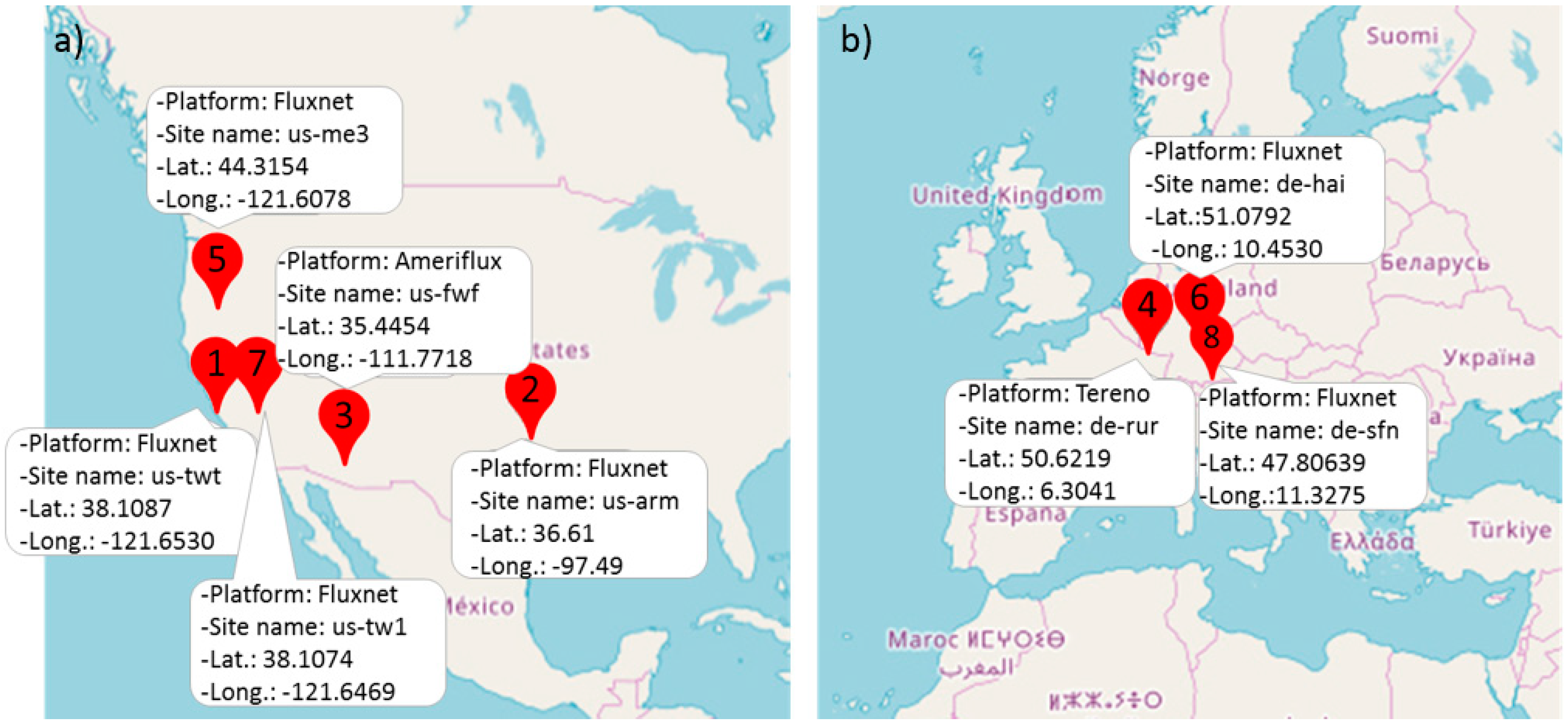
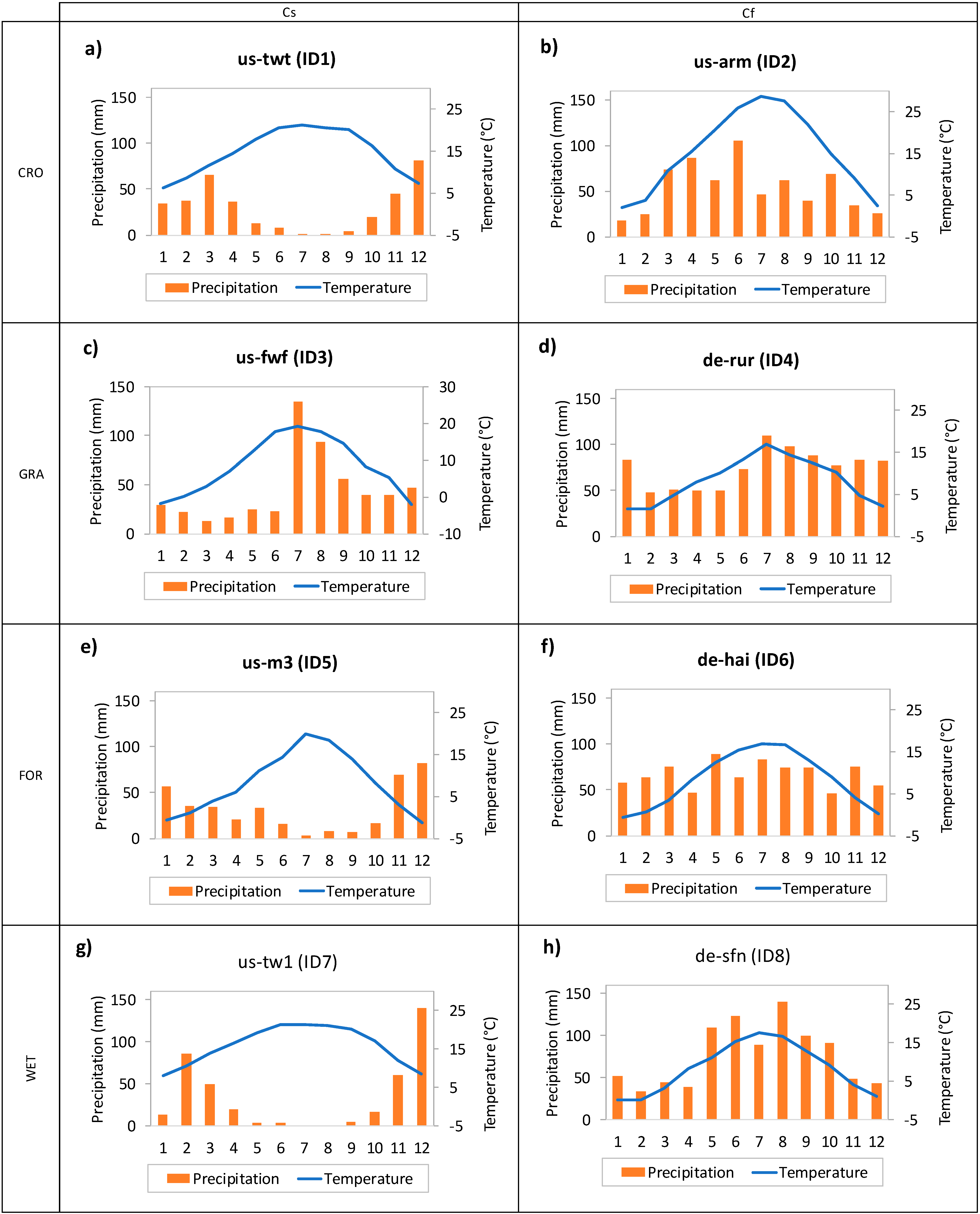
For this reason, additional studies in this field are encouraged. Within this framework, in the present study, a comparison among six approaches through eight experimental sites has been performed. Among the PET models, Priestley–Taylor (PT), Penman-Monteith (PM), and Blaney–Criddle (BC) approaches have been considered while among the AET models, the Advection-Aridity (AA) model, the Granger and Gray (GG) approach, and the Antecedent Precipitation Index (API) model have been selected. The eight experimental sites used for the comparison belong to the TERENO, AmeriFlux and FLUXNET networks. They are featured by different climate conditions including Mediterranean and temperate Oceanic climates, and different vegetation types which are grasslands (GRA), croplands (CRO), forests (FOR), and wetlands (WET). The performances of the six models for the eight experimental sites have been tested and compared with the aim of providing recommendations about the method which can be more effectively used with or without a calibration process and furthermore the impact and the importance of the calibration itself can be identified. Indeed, the calibration of the models to local conditions appears to be fundamental in order to reduce the errors resulting from the application of the approaches to regions different from those in which they were originally developed [38,42].

An additional work has consisted in the assessment of prediction errors of the proposed approaches when measured input parameters required for running the models, are not available and in their place estimated values from empirical relationships are used [41]. While meteorological data like precipitation and temperature are commonly measured by weather stations, other input parameters like net radiation or soil heat flux are less systematically covered by continuous measurement since more expensive measuring devices are required for this purpose (i.e., pyranometers, heat flux plates) [6].

The lack of these parameters makes challenging the use of several ET models narrowing the field of application only to temperature-based approaches [15,16,17,18]. Such restriction can be overcome by using empirical formulations to derive the missing parameters [41]. This is the case of several studies where meteorological data required for the implementation of ET models were not available and so indirect formulas were used. In detail, [38] due to the problem of meteorological variables availability in Poland, procedures and default coefficients suggested by [41] were used to derive ET with four radiation-based methods. Another example is [43], which due to the weather data limitation in Mediterranean areas, used standard empirical methods to calculate ET. When empirically derived meteorological variables are used, the accuracy of the ET predictions could vary considerably. In light of this, in the present paper, a comparison between the models performances using observed and modelled input variables has been performed.

2. Materials and Methods

2.1. The Experimental Sites

Observed ET data from eight eddy covariance (EC) towers have been used to compare the accuracy of the six selected models in predicting the evapotranspiration fluxes. The EC stations belong to three global networks namely Fluxnet (http://fluxnet.fluxdata.org/, accessed on 20 January 2021), TERENO (http://teodoor.icg.kfa-juelich.de/overview-en, accessed on 20 January 2021), and AmeriFlux (http://ameriflux.lbl.gov/, accessed on 20 January 2021) platforms. They are featured by different biomes which combine four different vegetation types (grassland, cropland, forest and wetland) and two climate conditions (Mediterranean, Oceanic).

For what concern the selection of the vegetation type, grasslands and forests have been considered since they are among the largest ecosystems in the world covering respectively about the 40% and 30% of the earth’s land area excluding Greenland and Antarctica [44,45]. Cropland has expanded rapidly in order to feed the world’s growing population [46] while wetland, although represents a small portion of the landscape, is found throughout the world [47]. Grassland ecosystems (GRA) are areas covered by grass-dominated vegetation with little or no trees and a variable intensity of meadows, steppes, and grasslands grazed. Cropland (CRO) is farmland with agricultural and/or horticultural products. The forest cover (FOR) includes terrestrial habitats dominated by trees and other woody plants. The wetland (WET) consists of permanent mosaic of water and herbaceous or woody vegetation. With respect to the climate, sites located in Mediterranean and Oceanic areas have been considered since they present very different temperature and precipitation annual patterns, with a marked seasonality in the case of the Mediterranean climate over the temperate Oceanic. Indeed, according to the Koppen classification, the Mediterranean climate (Cs) has mild, wet winters and warm-to-hot, dry summers with the precipitation mainly occurring during winter and autumn. The subtypes “Csa” and “Csb” represent a Mediterranean climate with average temperature respectively above and below 22° during the warmest month. The oceanic climate (Cf) is characterized by cool winters and warm summers, and the rainfall events are evenly dispersed during the year. Cf has the two subtypes “Cfa” and “Cfb” too. Eight areas with the considered biomes have been selected for the present study including “us-twt” (FLUXNET2015 DOI:10.18140/FLX/1440106) located on Twitchell island, Sacramento Country, California (USA) [48,49], “us-tw1” located on Twitchell island, Sacramento Country, California (USA) (FLUXNET2015 DOI:10.18140/FLX/1440108) [50,51,52], “us-arm” located near Billings, in northwest Noble County, Oklahoma (USA) (FLUXNET2015 DOI:10.18140/FLX/1440066) [53,54], “us-fwf” located near Flagstaff, Coconino County in Arizona (USA) (AMERIFLUX DOI:10.17190/AMF/1246052) [55,56], “de-rur” located in Simmerath, north Rhine-Westphalia (Germany) (https://deims.org/356417de-5a3c-429d-82c1-08a4e924ab3b, accessed on 20 January 2021) [57,58], “de-hai” located within the Hainich National Park in central Germany close to the city of Eisenach, western Thuringia (FLUXNET2015 DOI:10.18140/FLX/1440148) [59,60,61], “de-sfn” is located near Seeshaupt, Weilheim-Schongau district, in Bavaria, Germany (FLUXNET2015 DOI:10.18140/FLX/1440219) [62,63], “us-me3” located near Sisters, a city in Deschutes County, Oregon, United State (FLUXNET2015 DOI:10.18140/FLX/1440080) [64,65,66].

In Figure 1, the selected sites, the corresponding identification numbers (ID), location, and networks have been shown.

These sites have been preferred among all available locations with the required characteristics of climate and vegetation since they offer a better data quality standard, with longer periods of observation and low frequency in the occurrence of missing data that means a limited lack of measurements of latent heat flux (LE) (

Table 1. Percentage of missing latent heat flux (LE) values for each site.

ID	Name	Record Period	Number of Days	Number of 30 min Intervals	Missing LE (%)
1	us-twt	2009 to 2014	2098	100,704	32.4
2	us-arm	2003 to 2012	3653	175,344	11.8
3	us-fwf	2006 to 2010	1735	83,280	11.5
4	de-rur	2012 to 2017	2101	100,848	4.6
5	us-me3	2004 to 2009	2100	100,800	26.8
6	de-hai	2000 to 2007	2922	140,256	25.7
7	us-tw1	2012 to 2014	902	43,296	0.0
8	de-sfn	2012 to 2014	910	43,680	0.0

).

In details, the EC measurements inevitably include gaps within the time series of data recorded every 30 min. According to [67,68], the days with rates of missing data higher than 80% have been excluded by the analysis. The days with a percentage of gaps lower than the above-mentioned threshold, have been subjected to a standard gap-filling procedure, suggested by [69]. This approach replaces the missing values with the average value under similar meteorological conditions within a time-window of ±7 days. A summary of the percentages of missing data for the whole periods of observation and each site are provided in the Table 1 and in Table S1.

2.1.1. Climate Characterization of the Sites

Figure 2 illustrates the climate characterization for each of the selected sites, with the temporal patterns of the monthly average precipitation and air temperature computed over the periods of observation using data from the EC towers.

Figure 2 shows that us-twt station is characterized by minimum temperature of 6 °C occurring during December and maximum temperature of about 21 °C during July. The wettest month is December with 81 mm of rain fall while the driest month is July with no rain. The site has a typical Mediterranean climate (Csa) characterized by annual mean air temperature of 14.6 °C and mean annual precipitation of 344 mm.

The site “us-arm” is located in a humid subtropical (Cfa) area with mean annual temperature of 15.3 °C and mean annual precipitation of 646 mm. The mean monthly temperature and the precipitation range respectively from 2 °C (January) to 29 °C (July) and from 18 mm (January) to 105 mm (June).

The site “us-fwf” has a cool-summer Mediterranean climate (Csb) with an annual rainfall amount of 539 mm and a mean annual temperature of 8.4 °C. The monthly temperature reaches peaks of 19 °C during July and a minimum value of −2 °C in December while the monthly precipitation moves from 13 mm in March to 135 mm in July.

The test site of “de-rur” is located in an area with Oceanic (cfb) climate where the annual mean precipitation and air temperature are of approximately 895 mm and 8.4 °C. The monthly temperature varies from about 2 °C in February to 17 °C in July while the monthly precipitation from 48 mm to 110 mm during the same months.

The climate for us-me3 is temperate Mediterranean with a mean annual air temperature and precipitation of 8.2 °C and 384 mm respectively. The monthly temperature and precipitation reach minimum values of −1 °C (November) and 3 mm (July) and maximum values of 20 °C (July) and 82 mm (November).

The “de-hai” tower is located in a maritime temperate climate (Cfb) area with total annual depth of precipitation of about 806 mm and mean annual air temperature of about 8.3 °C. The lowest monthly temperature is of −0.5 °C and it is reached during January while the highest is 17 °C in August. The monthly precipitation ranges between 46 mm in October and 89 mm in May.

“Us-tw1” is featured by a Mediterranean climate (Csa) with mean annual temperature of 15 °C and a total annual precipitation volume of 399 mm. During July no rain falls while December is the wettest month with 140 mm of precipitation. The temperature reaches maximum and minimum monthly values respectively of 8 °C (January) and 21 °C (June). The “de-sfn” station is located in an area with temperate climate (Cfb). The mean annual air temperature and precipitation are 8.3 °C and 914 mm respectively. The hottest month is July with average temperature of 18 °C while the coldest is February with 0.1 °C. The rain falls most during August (140 mm) while it reaches its lowest value during February (34 mm).

The moisture index (I_M) proposed by Thornthwaite [16] has been calculated for each investigated site so as to provide a more detailed climate characterization. It can be estimated as:

$$I_M = \frac{P-PET}{PET}·100$$

(1)

where:

P and PET respectively represent the average annual precipitation and potential evapotranspiration which is given by the sum of monthly PET_i values computed as:

$$PE{T}_i = 1.6·{\left(\frac{10·T_i}{I}\right)}^a$$

(2)

where T_i is the average air temperature during the i-th month of the year (in degree Celsius) while I is the annual heat index got from the summation of monthly heat indices i:

$$i_i = {\left(0.2·T_i\right)}^{1.514}$$

(3)

The coefficient a is evaluated as:

$$a = 6.75·{10}^{-7}·I^3-7.771·{10}^{-5}·I^2 + 0.01792·I + 0.49239$$

(4)

In

Table 2. Climatic types and the corresponding ranges of I_M.

Climatic Type	IM
(A) Perhumid	IM > 100
(B4) Very humid	80 < IM ≤ 100
(B3) Highly humid	60 < IM ≤ 80
(B2) Moderate humid	40 < IM ≤ 60
(B1) Low humid	20 < IM ≤ 40
(C2) Moist subhumid	0 < IM ≤ 20
(C1) Dry subhumid	−20 < IM ≤ 0
(D) Semiarid	−40 < IM ≤ −20
(E) Arid	IM ≤ −40

for each climate type, the corresponding range of I_M values has been defined.

2.1.2. The Land Cover Type of the Sites

The site us-twt is located on a cultivated crop consisting of rice planted at a density of 14–17 g m⁻². The tower “us-arm” lies on a land primarily covered by winter wheat and grass-land/pasture. The EC station us-fwf is above an area covered by forest converted to grassland by intense burning in 1996 so currently, the trees density is of 0 trees ha⁻¹. The vegetation after the fire, consisted of sparse grasses, forbs, and shrubs. De-rur is a grassland site. The composition of higher plant species at the site is typical for traditionally managed grasslands and consists of Ranunculus repens–Alopecurus pratensis plant community, where a majority of species are identified as meadow foxtail, perennial rye grass, rough meadow grass, and common sorrel. The land biome of us-me3 is almost exclusively composed of young ponderosa pine trees with a density lower than normally found in similar ecosystem. De-hai is a forest area which is primarily composed by beech with smaller percentage of ash, maple, and other deciduous and coniferous species. The forest has a tree density of about 330 trees ha⁻¹. Us-tw1 eddy covariance station is located in an area with vegetation including hydrophytic plants with emergent marsh species like Schoenoplectus acutus and Typha species. A relatively greater proportion of vegetation consists of S. acutus stems 1–3 m tall. The site of de-sfn is a natural bog-pine forest where the vegetation is quite heterogeneous and includes peat mosses (Sphagnum spp.) in addition to heather (Calluna vulgaris L.), bog bilberry scrubs (Vaccinium uliginosum L.s.l.) and several species of the sedge-family (Cyperaceae, mainly Eriophorum vaginatum L., hare’s-tail cottongrass).

2.1.3. Instrumentation and Dataset

Meteorological daily data used to run the selected ET prediction models are net solar radiation, air temperature, relative humidity, wind speed, latent heat flux, precipitation, and soil heat-flux density. Actual evapotranspiration has been calculated from the latent heat flux using the procedure suggested by FAO [41]:

$${ET}_{EC} = \frac{\mathrm{LE}}{\lambda }$$

(5)

where ET_EC represents the actual evapotranspiration flux (mm⁻¹), LE is the latent heat flux (Mj m⁻²d⁻¹), λ is the latent heat of vaporization (MJ kg⁻¹).

The above-said measurements have been collected by the monitoring systems at the different sites at hourly and sub-hourly timescale and then aggregated at daily scale which is the scale of analysis used in the present analysis.

The instrumentation of each site is briefly described in the following. In the site us-twt, the fluxes of carbon dioxide, methane, latent heat, and sensible heat have been measured using the EC method while a sonic anemometer allows to measure wind speed and temperature at the measurement height of 3.05 m. The station us-arm is equipped with a sonic anemometer (Gill-Solent WindMaster Pro), an open-path infrared gas analyzer (IRGA LiCorLI-7500), and a set of meteorological and soil sensors which allow to monitor radiation, wind speed and direction, air temperature and humidity, precipitation, soil heat flux. The measurement height is 4 m. In the site us-fwf, the measurements have been performed using a 3D sonic anemometer (CSAT3, Campbell Scientific, Logan, UT, USA), a closed path CO₂/H₂O analyzer (Li-7000, Li-Cor, Lincoln, NE, USA) at the height of 60 m.a.s.l. Additionally air and soil meteorological measurements have been recorded. The test-site de-rur includes a 2.6 m-high eddy covariance tower, installed since 2011 with a sonic anemometer and an infrared gas analyzer. Eddy-covariance measurements at us-me3 station have been collected using a three-dimensional sonic anemometer and an open-path infrared gas analyzer with additional measurements including atmospheric temperature, relative humidity, and precipitation. The eddy-covariance data were collected at the height of 12 m. At de-hai site, using the eddy covariance technique, water vapor, heat. and momentum fluxes have been continuously measured at a height of about 43 m.a.s.l. The equipment consisted of a triaxial sonic anemometer (Gill Solent R3, Gill Instruments, Lymington, UK) and a CO₂ and water infrared gas analyzer (LiCor 6262–3, LiCor Inc., Lincoln, NE, USA). In addition, the tower measured wind direction and velocity, air humidity and air temperature, radiation and precipitation. The tower of us-tw1 is equipped to analyze energy, H₂O, CO₂, and CH₄ fluxes. Fluxes are measured in detail using an open-path infrared gas analyzer (LI-7500 or LI-7500 A for CO₂ and H₂O, LI-7700 for CH4, LiCOR Inc., Lin-coln, NE, USA). In addition, the air temperature and three-dimensional wind speeds are measured with a sonic anemometer (WindMaster Pro 1352 or 1590, Gill Instruments Ltd., Lymington, Hampshire, England). The eddy-covariance data at de-sfn test site are collected at the height of 6 m. The flux measurements are collected using an open-path infrared gas analyzer (IRGA, LI7500, Li-Cor, Inc., Lincoln, NE, USA) in addition, a 3-D sonic anemometer (CSAT-3, Campbell Scientific, Inc., Logan, UT, USA), a heated tipping bucket rain gauge 52202 (Campbell Scientific), and a heated and ventilated CNR4 (Kipp and Zonen, Delft, The Netherlands) are currently in use.

The monitoring period differs from site to site (

Table 3. Detail for the selected sites.

ID	Name	Lat./Long.	Vegetation Type	Elevation (m)	Record Period	Climate	Mean Annual Temperature (°C)	Mean Annual Precipitation (mm)
1	us-twt	38.1087/−121.6530	CRO	0	2009 to 2014	Csa	14.6	344
2	us-arm	36.61/−97.49	CRO	314	2003 to 2012	Cfa	15.3	646
3	us-fwf	35.4454/−111.7718	GRA	2270	2006 to 2010	Csb	8.4	536
4	de-rur	50.6219/6.3041	GRA	514.7	2012 to2017	Cfb	8.4	895
5	us-me3	44.3154/−121.6078	FOR	1005	2004 to 2009	Csb	8.2	384
6	de-hai	51.0792/10.4530	FOR	430	2000 to 2007	Cfb	8.3	806
7	us-tw1	38.1074/−121.6469	WET	−5	2012 to 2014	Csa	15.9	399
8	de-sfn	47.80639/11.3275	WET	590	2012 to 2014	Cfb	8.3	914

), the shortest one refers to sites us-tw1 and de-sfn where two years of measurements (from 2012 to 2014) are available while the longest period of observation ranging from 2003 to 2012, is related to the site us-arm. In the following table a summary of the characteristics of the test-sites can be found.

2.2. Description of the Selected AET and PET Models and Their Evaluation

ET predictions from six models have been compared with the measured data. Three PET models and three AET methods have been selected. The description of these models is available in the following.

2.2.1. PET Approaches

The combination-type model suggested by Penman–Monteith (PM), the radiation-based approach of Priestley–Taylor (PT), and the temperature-based formula proposed by Blaney–Criddle (BC) have been used in the present study to model PET. PM is probably the most commonly used method in the scientific literature to derive potential evapotranspiration [70]. The PM method assumes that all the energy for evaporation can be used by the plants and that water first has to pass through stomata openings, total leaf area, and soil surface against surface resistance and then it diffuses into the atmosphere against the aerodynamic resistance [71]. Since PM approach takes into account the heat and water vapor mass transfer mechanisms, it is considered a combination equation. The PM equation is:

$$PE{T}_{PM} = \frac{1}{\lambda }\left[\frac{\Delta }{\Delta + \gamma }\left(R_n-G_{soil}\right)\right] + \left[\frac{\gamma }{\gamma + \Delta }{E}_A\right]$$

(6)

where Δ is the slope of the saturation vapor pressure–temperature curve (kPa °C⁻¹) expressed as:

$$\Delta = \frac{4098\left[0.6108\exp \left(\frac{17.27·{\mathrm{T}}_{\mathrm{mean}}}{{\mathrm{T}}_{\mathrm{mean} + 237.3}}\right)\right]}{{\left(237.3 +{ \mathrm{T}}_{\mathrm{mean}}\right)}^2}$$

(7)

T_mean represents the average temperature between maximum and minimum values during the day (°C), λ is the latent heat of vaporization (MJ kg⁻¹), γ is the psychrometric constant (kPa °C⁻¹), and E_A is the drying power of the air given by the following formula:

$$E_A = 2.6\left(1 + 0.54u\right)\left({\mathrm{e}}_{\mathrm{s}}-{\mathrm{e}}_{\mathrm{a}}\right)$$

(8)

where u is the wind speed (ms⁻¹), 2.6(1 + 0.54·u) represents a function of the wind f(u), e_s and e_a are respectively the saturation vapor pressure (kPa) and the vapor pressure (kPa), Rn is the net radiation (MJ m⁻² d⁻¹) and Gsoil is the soil heat-flux density at the soil surface (MJ m⁻² d⁻¹) which can be considered to be negligible at daily time scale [41] as in the case of the sites ID5 and ID7 where measured values are not available.

Priestley–Taylor (PT) model was developed for the prediction of potential evaporation fluxes from a wet vegetated surface under conditions of minimum advection [72,73,74]. It simplifies the PM equation removing the aerodynamic component, when the surrounding environment is wet or humid conditions prevail. Priestley–Taylor [12] equation is given by:

$$PE{T}_{PT} = \frac{1}{\lambda }·\alpha \left[\frac{\Delta }{\Delta + \gamma }\left(R_n-G_{soil}\right)\right]$$

(9)

where α is the advection correction coefficient and it is set at the value of 1.26.

The Blaney–Criddle (BC) model is a simpler alternative to the PM and PT equations since it requires only mean temperature for monthly ET assessment. The usual form of the BC equation is:

$$PE{T}_{BC} = p·\left(0.46·{\mathrm{T}}_{\mathrm{mean}} + 8\right)$$

(10)

where p is the mean percentage of total daytime hours (at daily or monthly scale depending on the considered period) and it is unitless.

2.2.2. AET Models

In the present study, AET fluxes have been estimated using three meteorological data-based approaches including the Advection Aridity (AA) model, the Granger and Gray (GG) model, and the Antecedent Precipitation Index (API) model. The AA approach [26] and the GG method [29] belong to the category of complementary relationship (CR) models and are among the most used within this class. The AA formulation can be written as:

$$AE{T}_{AA} = \left(2\alpha -1\right)\frac{1}{\lambda }\left[\frac{\Delta }{\Delta + \gamma }\left(R_n-G_{soil}\right)\right]-\left[\frac{\gamma }{\gamma + \Delta }{E}_A\right]$$

(11)

The present equation combines an aerodynamic term with an energy component based on net incoming radiation.

According to Granger and Gray [29], AET can be calculated using the following equation:

$$AE{T}_{GG} = \left[\frac{\Delta ·G}{\Delta + \gamma }\left(\frac{R_n-G_{soil}}{\lambda }\right)\right] + \left[\frac{\gamma ·G}{\gamma + \Delta ·G}{E}_A\right]$$

(12)

It describes ET from non-saturated surfaces. In order to account for the departure from saturated conditions, Equation (12) applies the concept of relative evaporation introduced by the use of G, the relative evaporation parameter expressed as:

$$G = \frac{1}{0.793 + 0.20e^{4.902D}} + 0.006D$$

(13)

where D is the relative drying power:

$$D = \frac{E_A}{E_A + R_n}$$

(14)

AET has been also estimated using the API model. Mawdsley and Ali [21] modified the Priestley–Taylor model for the estimation of non-potential evapotranspiration. They found that the parameter α was affected by water shortages, which can be described as a function of soil moisture [75]. Because surface soil moisture is not routinely available, they used the API index [76] to mimic soil moisture conditions:

$$API = {\displaystyle \sum }_{t = -1}^{-i}{P}_t{k}^{-t}$$

(15)

where i is the considered number of days which precede the day t, k is an empirical decay factor, and $P_t$ is the rainfall for the day t.

The non-potential evapotranspiration fluxes can be calculated using the following formulation:

$$AE{T}_{API} = \frac{1}{\lambda }·{\alpha }_{API}\left[\frac{\Delta }{\Delta + \gamma }\left(R_n-G_{soil}\right)\right]$$

(16)

In the previous equation, α_API is a dimensionless coefficient and it is a function of API. In particular, when API is lower than or equal to 20 mm [21], α_API can be expressed as:

$${\alpha }_{API} = 0.123\left(API\right)-0.0029{\left(API\right)}^2-0.0000056{\left(API\right)}^3$$

(17)

When API is higher than 20 mm:

$${\alpha }_{API} = 1.26$$

(18)

assuming that for an over-saturated system (i.e., API > 20 mm), AET rates are no longer dependent on the soil water content, but they are a constant percentage of PET.

2.2.3. Calibration of the Models for the Prediction of AET

The need for a calibration procedure of the AET approaches which involves the models parameters and which is able to increase the accuracy of the ET predictions, has been confirmed in time by several scholars [77,78]. In general, the calibration procedure of the AA model involves the wind function f(u) and the α-coefficient, for GG method the calibration parameter is the relative evaporation G, while for API method, α-coefficient is subjected to the calibration process. The scientific literature suggests a moderate range of variability for these parameters. With regard to the α-coefficient, it has been found to vary between 1.05 and 2.20 [79,80]. Concerning the wind function, many researches proposed different values of aw and bw such as aw = 0.37 and bw = 0.22 [81], aw = 1.313 and bw = 1.381 [6], or aw = 0.1954 and bw = 0.4703 [82]. With respect to the parameter G, several authors indirectly derived it in time [83,84].

In the present research, a one-step calibration procedure has been performed for API and the GG models, where the best fitting between monthly observed ET (ET_EC) and modelled ET has been reached by minimizing the model errors. The calibration procedure concerning the AA approach is a two-step process [82,85] because the formulation of the model has a two-term structure.

The term linked to the drying power of advected air has been calibrated discarding the data of the dry days identifiable as those with a soil water content lower than the fixed threshold of 20% [86]. The wind function has been iteratively calibrated until reaching the best fitting between the observed and modelled ET during the well-watered days. Subsequently, the α-coefficient has been calibrated considering both the wet and dry days and so, the whole period of observation.

2.2.4. The Indirect Estimates of Net Radiation and Soil Heat-Flux

According to Allen et al. [41], the variables Rn and Gsoil, if not available from in situ measurements, can be derived by the following empirical relationships:

$$Rn = Rns-Rnl$$

(19)

where Rns is net shortwave radiation and Rnl is the outgoing net longwave radiation and can be respectively expressed as:

$$\{\begin{array}{c}Rns = \left(1-\beta \right)Rs\\ Rnl = {\sigma }_{SB}\left[\frac{T_{max,K^4} + T_{min,K^4}}{2}\right]\left(0.34-0.14\sqrt{e_a}\right)\left(1.35\frac{Rs}{Rso}-0.35\right)\end{array}$$

(20)

where Rs is the incoming solar radiation, β is the canopy reflection coefficient, σ_SB is the Stefan–Boltzmann constant, T_max,K and T_min,K are respectively the maximum and minimum absolute temperature during the 24 h period, Rso is the clear-sky solar radiation. Rs and Rso can be calculated as follows:

$$\{\begin{array}{c}Rs = \left(a_s + b_s\frac{n}{N}\right)Ra\\ Ra = \frac{12\left(60\right)}{\pi }{G}_{sc}{d}_r\left[\left({\omega }_2-{\omega }_1\right)\sin \phi \sin \delta + \cos \phi \cos \delta \left(\sin {\omega }_2-\sin {\omega }_1\right)\right]\\ Rso = \left(0.75 + 2·{10}^{-5}z\right)Ra\end{array}$$

(21)

In the previous equations, as and bs are regression constants, expressing the fraction of extraterrestrial radiation reaching the earth on overcast days, n represents the actual duration of sunshine, N is the symbol for the maximum possible duration of sunshine or daylight hours, Ra is the extraterrestrial radiation in the hour, G_sc indicates the solar constant, d_r expresses the inverse relative distance Earth–Sun, ω₁ and ω₂ respectively are the solar time angle at beginning and at end of period, φ is the latitude, δ solar declination, z is the station elevation above sea level.

The equation of soil heat-flux density at the soil surface is:

$$G_{soil} = c_s\frac{T_i-T_{i-1}}{\Delta t}\Delta y$$

(22)

where c_s indicates the soil heat capacity, T_i and T_i−1 respectively are the air temperature at time i and i − 1, Δt is the selected time interval, Δy is the effective soil depth.

2.2.5. Models Evaluation

The evapotranspiration losses computed at monthly scale using the selected models have been compared to the observed values of ET from the eddy-covariance towers so as to estimate the accuracy of each approach. The comparison allows to test the performances of the models in simulating the actual ET fluxes. The goodness-of-fit indices used for the comparison are the normalized root mean square error (RMSEd) which measures the error intensity, the index of agreement (d) which measures the patterns agreement, the correlation coefficient (r) which estimates the correlation between measured and simulated variables. The corresponding equations are:

$$RMSE \left(\mathrm{mm}\right) = {\left[\frac{1}{n}{\displaystyle \sum }_{i = 1}^n{\left(E{T}_{mod,i}-E{T}_{EC,i}\right)}^2\right]}^{\frac{1}{2}}$$

(23)

$$RMSEd (-) = \frac{RMSE \left(\mathrm{mm}\right)}{{\overline{ET}}_{EC}}$$

(24)

$$d(-) = 1-\frac{{\sum }_{i = 1}^n\left|E{T}_{mod,i}-E{T}_{EC,i}\right|}{{\sum }_{i = 1}^n\left(\left|E{T}_{mod,i}-{\overline{ET}}_{EC,i}\right| + \left|E{T}_{obs,i}-{\overline{ET}}_{EC,i}\right|\right)}$$

(25)

$$r(-) = \frac{Cov\left(E{T}_{mod},E{T}_{EC}\right)}{\sigma \left(E{T}_{mod}\right)\sigma \left(E{T}_{EC}\right)}$$

(26)

where n is the length of the monthly sample, ET_mod,i is the monthly modelled ET value while ET_EC,i is the observed one from EC measurements, and σ the ET standard deviation.

3. Results

3.1. Results of the Climate Investigation

The values of the moisture index (I_M) (

Table 4. Value of the moisture index for each site.

ID	Name	IM (-)	Climatic Type
1	us-twt	−65	Arid
2	us-arm	−40	Arid
3	us-fwf	−7	Dry sub-humid
4	de-rur	68	Highly humid
5	us-me3	−30	Semi-arid
6	de-hai	47	Moderate Humid
7	us-tw1	−62	Arid
8	de-sfn	64	Highly humid

) calculated for each test site, suggest that four sites can be classified as arid or semi-arid including us-twt, us-arm, us-me3, us-tw1 while us-fwf, de-rur, de-hai, and de-sfn can be listed among the humid and sub-humid climatic types. In details, the most arid site is us-twt with a value of I_M of −65 while the most humid is de-rur with I_M of 68.

From Figure 2, it can be deduced that the site with the highest annual rainfall is de-sfn with 914 mm followed by de-rur with 895 mm. The area with the lowest annual precipitation is us-twt with 344 mm of rain fallen but similar values have been reached by us-me3 and us-tw1 respectively with 384 and 399 mm of cumulative rainfall.

The site with the highest mean annual temperature is us-arm with 15.3 °C while the lowest temperature (8.2 °C) occurs in the test site of us-me3.

In addition, from Figure 2 it emerges clearly that the Mediterranean areas present a seasonal variation of rainfall patterns indeed, most of the precipitation occurs in winter months followed by a dry period during summer. On the other side, the Oceanic areas show precipitation with an even distribution throughout the year. In both climates, the temperature reaches peak during the summer months from July to August while the coldest months are November, December, January, and February.

3.2. Results of the Montlhy Predictions Using the Selected ET Models

The evapotranspiration fluxes estimated by the six models and using the measured input parameters show similar temporal patterns (Figure 3) even if the observed ET values are significantly overestimated. This occurs for all sites except for the de-rur.

The values of the goodness-of-fit indices used for the quantitative assessment of models accuracy in the prediction of ET fluxes at monthly scale are shown in

Table 5. Goodness of fit indices computed for each approach and site. In bold the most accurate model for each site.

		Measured Rn and Gsoil			Modelled Rn and Gsoil
Site	Models	RMSE d (-)	d (-)	r (-)	RMSE d (-)	d (-)	r (-)
us-twt (CRO-Csa) ID1	API	0.42	0.73	0.83	0.50	0.68	0.71
	AA	0.43	0.69	0.80	0.52	0.62	0.85
	GG	0.29	0.81	0.91	0.43	0.72	0.84
	PM	0.67	0.63	0.87	0.87	0.52	0.82
	PT	0.26	0.82	0.93	0.40	0.76	0.86
	Blaney-Criddle	0.54	0.57	0.91	0.54	0.57	0.91
us-arm (CRO-Cfa) ID2	API	1.24	0.47	0.69	2.26	0.23	0.63
	AA	0.67	0.57	0.70	1.39	0.45	0.66
	GG	1.12	0.49	0.71	2.09	0.21	0.66
	PM	2.54	0.18	0.58	3.40	0.14	0.55
	PT	1.24	0.47	0.69	2.27	0.23	0.63
	Blaney-Criddle	2.21	0.19	0.61	2.21	0.19	0.61
us-fwf (GRA-Csb) ID3	API	0.95	0.55	0.82	3.01	0.17	0.82
	AA	0.63	0.54	0.85	1.86	0.37	0.85
	GG	1.21	0.48	0.77	3.06	0.16	0.80
	PM	2.68	0.19	0.70	4.37	0.12	0.74
	PT	0.97	0.53	0.81	3.04	0.17	0.82
	Blaney-Criddle	2.05	0.22	0.83	2.05	0.22	0.83
de-rur (GRA-Cfb) ID4	API	0.18	0.89	0.99	0.55	0.72	0.98
	AA	0.29	0.80	0.97	0.45	0.77	0.96
	GG	0.21	0.87	0.99	0.51	0.72	0.98
	PM	0.41	0.74	0.99	0.75	0.58	0.99
	PT	0.20	0.88	0.99	0.55	0.72	0.98
	Blaney-Criddle	1.23	0.33	0.98	1.23	0.33	0.98
us-me3 (FOR-Csb) ID5	API	1.94	0.37	0.75	2.32	0.29	0.82
	AA	1.28	0.49	0.79	1.74	0.41	0.85
	GG	1.97	0.35	0.72	2.31	0.27	0.80
	PM	2.78	0.24	0.66	3.09	0.20	0.73
	PT	1.99	0.36	0.72	2.37	0.28	0.80
	Blaney-Criddle	2.67	0.19	0.73	2.67	0.19	0.73
de-hai (FOR-Cfb) ID6	API	1.34	0.59	0.96	2.00	0.41	0.96
	AA	0.81	0.75	0.94	1.49	0.56	0.95
	GG	1.41	0.56	0.95	1.97	0.39	0.96
	PM	2.05	0.38	0.95	2.61	0.28	0.95
	PT	1.34	0.59	0.96	2.00	0.41	0.96
	Blaney-Criddle	3.43	0.20	0.96	3.43	0.20	0.96
us-tw1 (WET-Csa) ID7	API	0.82	0.54	0.41	0.82	0.53	0.40
	AA	0.38	0.74	0.86	0.36	0.75	0.87
	GG	0.50	0.73	0.83	0.52	0.71	0.84
	PM	0.83	0.55	0.82	0.86	0.53	0.83
	PT	0.49	0.74	0.84	0.51	0.72	0.85
	Blaney-Criddle	0.60	0.53	0.88	0.60	0.53	0.88
de-sfn (WET-Cfb) ID8	API	1.10	0.55	0.95	2.42	0.30	0.95
	AA	0.99	0.62	0.96	2.58	0.32	0.95
	GG	1.01	0.57	0.95	2.08	0.33	0.95
	PM	1.27	0.48	0.94	2.30	0.29	0.95
	PT	1.11	0.55	0.95	2.44	0.30	0.95
	Blaney-Criddle	1.92	0.28	0.71	1.92	0.28	0.71

, both in case of measured/observed and empirically-derived Rn and Gsoil. In addition, in Table 5, the most accurate model is indicated for each site. In general, the AET models are better able to reproduce the ET measurements than PET approaches with maximum values of RMSEd at most of 1.97 against 3.34 of PET models. In particular, in almost all sites, the best performing approach appears to be the AA model with average values of RMSEd, d, and r respectively of 0.8, 0.6, and 0.9. A reduction of the prediction accuracy can be observed when the indirect evaluation of Rn and Gsoil has been performed. In this case, the best performing methods exhibit values of RMSEd close to 2 and agreements lower than 0.5 although with high values of r.

A summary of the goodness of fit indices referring to the non-calibrated best performing approach for each site and with reference to the specific land cover type and climate condition has been reported in Figure 4. The highest prediction errors are reached for forest ecosystems and arid/semiarid conditions where the values of RMSEd are close to 1.2 while the grassland environments and the humid/sub-humid climates present the better accuracy with RMSEd around 0.2.

In case of lack of measurements of Rn and Gsoil, these variables are estimated using empirical formulas. The errors between observed and modelled Rn and Gsoil are shown in

Table 6. The RMSEd for the modelled Rn and Gsoil variables.

Site	RMSEd_Rn (-)	RMSEd_Gsoil (-)
ID1	0.36	21.94
ID2	0.70	−1.72
ID3	1.31	3.68
ID4	0.46	−10.77
ID5	0.52	-
ID6	0.45	−23.66
ID7	0.07	-
ID8	0.75	−46.87

. The error ranges from a minimum value of 0.07 to a maximum value of 1.31 for the net radiation while it moves between −46.87 and 3.68 for the soil heat-flux density. So, the error made in estimating Gsoil is persistently higher than the one related to Rn.

Besides the quantitative aspect, the temporal patterns of monthly observed Rn and Gsoil plotted against the modelled ones are shown in Figure 5. The figure reveals, at first sight, that they differ both in terms of temporal dynamics and magnitude.

3.3. Results of the Calibration Procedure

A site-specific calibration procedure has been performed in order to reduce the prediction errors of the selected models. The model calibration has involved a scenario where Rn and Gsoil were directly measured and not provided by the use of empirical formulas in order to avoid even larger models distortion. Since the AET models have returned better performances than PET approaches, the calibration procedure has been performed only for AA, API, and GG models (AA_cal, API_cal, and GG_cal). The values of α-coefficient and the formulations of the wind function and of the relative evaporation parameter for each site after the calibration procedure (respectively α_CAL, f(u)_CAL and G_CAL) are shown in

Table 7. Goodness of fit indices for the eight experimental sites. The most accurate models in case of calibrated and non-calibrated approach are compared (Table 5).

Site	Models	RMSEd (-)	d (-)	r (-)	Calibrated Parameters
us-twt (CRO-Csa) ID1	APIcal	0.25	0.84	0.93	αcal = 1.33
	AAcal	0.32	0.81	0.92	αcal = 1.46; f(u)cal = 3.2(1 + 0.029u)
	GGcal	0.27	0.84	0.92	Gcal = 1/(1.5 + 3∙10−6e27.3D) + 0.044∙D
	PT	0.26	0.82	0.93	-
us-arm (CRO-Cfa) ID2	APIcal	0.48	0.61	0.69	αcal = 0.57
	AAcal	0.64	0.50	0.73	αcal = 1.22; f(u)cal = 4.3(1 + 0.02u)
	GGcal	0.43	0.68	0.77	Gcal = 1/(0.55 + 0.035 e13.02D) + 0.061∙D
	AA	0.67	0.57	0.70	-
us-fwf (GRA-Csb) ID3	APIcal	0.38	0.73	0.82	αcal = 0.77
	AAcal	0.47	0.71	0.80	αcal = 1.30; f(u)cal = 4.2(1 + 0.012u)
	GGcal	0.39	0.72	0.80	Gcal = 1/(0.77 + 1.68e3.15D) + 0.0881∙D
	AA	0.63	0.54	0.85	-
de-rur (GRA-Cfb) ID4	APIcal	0.15	0.90	0.99	αcal = 1.22
	AAcal	0.21	0.87	0.98	αcal = 1.25; f(u)cal = 2.53(1 + 0.054u)
	GGcal	0.13	0.91	0.99	Gcal = 1/(1.2 + 0.2e4.3D) + 0.012∙D
	API	0.18	0.89	0.99	-
us-me3 (FOR-Csb) ID5	APIcal	0.59	0.65	0.73	αcal = 0.57
	AAcal	0.65	0.64	0.78	αcal = 0.92; f(u)cal = 1.88(1 + 0.0035u)
	GGcal	0.47	0.72	0.80	Gcal = 1/(3.63 + 0.005e22.62D) + 0.07∙D
	AA	1.28	0.49	0.79	-
de-hai (FOR-Cfb) ID6	APIcal	0.30	0.87	0.96	αcal = 0.56
	AAcal	0.42	0.84	0.95	αcal = 1.03; f(u)cal = 3.10(1 + 0.0005u)
	GGcal	0.24	0.89	0.96	Gcal = 1/(3.93 + 0.395e4.09D) + 0.0069∙D
	AA	0.81	0.75	0.94	-
us-tw1 (WET-Csa) ID7	APIcal	0.38	0.73	0.84	αcal = 0.96
	AAcal	0.37	0.74	0.84	αcal = 1.19; f(u)cal = 1.544(1 + 0.003u)
	GGcal	0.38	0.73	0.84	Gcal = 1/(4.45 + 4 × 10−6e32D) + 0.4413∙D
	AA	0.38	0.74	0.86	-
de-sfn (WET-Cfb) ID8	APIcal	0.29	0.85	0.95	αcal = 0.59
	AAcal	0.75	0.55	0.96	αcal = 0.74; f(u)cal = 1.2722(1 + 0.003u)
	GGcal	0.26	0.84	0.95	Gcal = 1/(2.19 + 1.18e7.5D) + 0.6628∙D
	AA	0.99	0.62	0.96	-

. For the sites ID1 and ID4, the values of α_CAL resulting from the calibration of API approach are close to 1.26 where for the other sites, they are significantly different from this standard coefficient. With regard to the values of α_CAL resulting from the calibration of AA approach, they are more likely similar to 1.26. For the experimental sites ID4 and ID6, the formulations of G, after the calibration process, approach the original one while this does not happen for the other sites. Concerning the parameter b_w of the wind function, the calibration procedure returns for all sites, a value ten times lower than the original one of 0.54.

The predictions of AET fluxes resulting from the calibrated models (API_CAL, AA_CAL, GG_CAL) and from the most accurate non-calibrated models have been compared using the selected goodness of fit indices (Table 7).

In general, the calibrated models present lower error than the most accurate models in case of non-calibrated approach. In Figure 6, the monthly patterns of the ET losses modelled using the calibrated approaches are illustrated along with the observed ET values and the ones from the most accurate non-calibrated method for each site and, at a fist visual inspection, it is possible to discern an improvement in ET estimates related to the calibration procedure.

The relative difference in RMSE, r, and d before and after the calibration procedure as shown in Figure 7, allows to observe that the error decreases due to this process indeed, when the difference in RMSE is positive, the model performances improve and vice versa for d and r.

In Figure 8, it is possible to observe in which kind of climatic condition and land cover, the calibrated models exhibit the worst performances in terms of RMSE, d, and r. The forest systems and the arid/semi-arid climates are confirmed to have the lowest performances also in case of calibrated approach.

4. Discussion

The findings illustrated in the previous chapter highlight various aspects which can be summarized as follows.

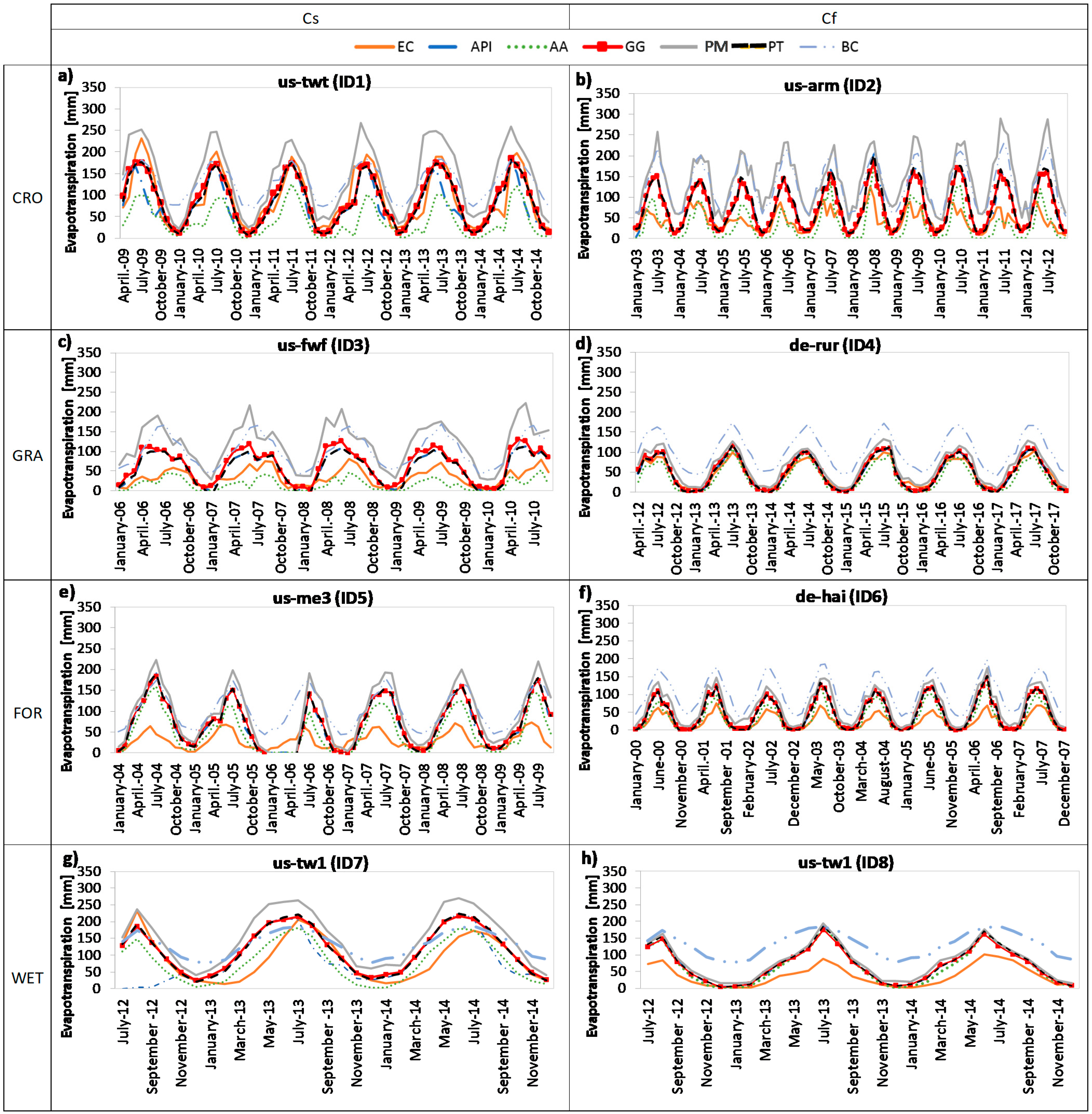
PET approaches are less accurate than AET models since the ET estimates computed using these methods significantly overestimate the observed ET with high RMSE even if r is quite high too. Actually, among PET models, Priestley–Taylor method exhibits the best performances, so it represents an exception to the rule. It shows an accuracy comparable to the API model used for the prediction of AET and in addition, for the site us-twt (ID1), PT model is the most accurate.

Among the AET models, the AA approach presents the highest performances for most of the studied sites (ID 2,3,5,6,7,8) and comparable in the others (ID 1,4) while API model is the most accurate for the prediction of monthly ET for the site of de-rur (ID4). Anyway, it should be noted that, for de-rur, all the AET models present similar performances (Table 4).

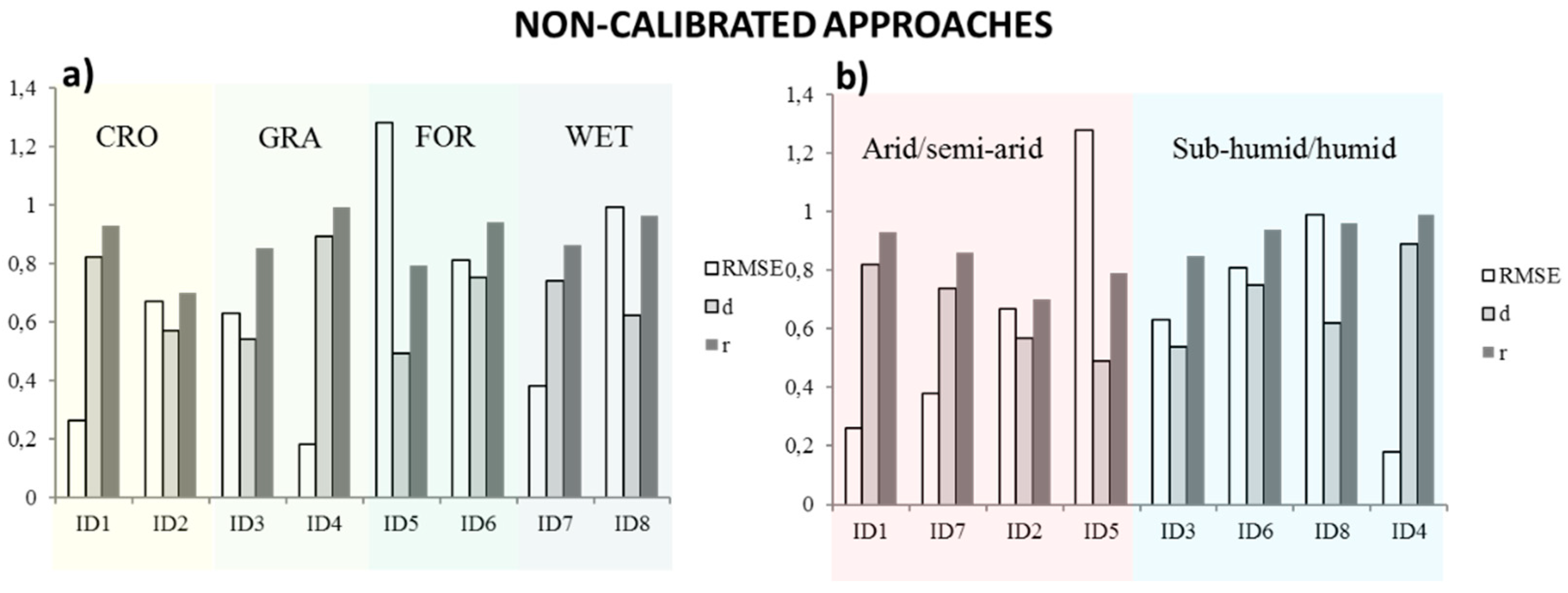
With regard to the land cover type, the highest values of RMSE and the lowest values of r and d occur for the forest cover type systems (ID5 and ID6) (Figure 4 left panel).

This result has been confirmed by previous investigations which documented a lower accuracy of the ET models in predicting the evapotranspiration fluxes for forest sites [37,87]. The reason could lie in the fact that the proposed models do not have correction terms which take into account the roughness sub-layer (RSL) effects typical of tall canopy-like forest ecosystems. The roughness sub-layer (RSL) is the lowest atmospheric layer immediately adjoining an area covered with roughness elements like trees. It extends from the forest vegetation height up to about twice that height. The EC towers allows measurements inside this layer but for these measurements, the classical method of the flux gradient relationship based on the surface-layer theory, fails and modifications to the methods are required in order to consider the RSL effect [88,89].

Another reason could be linked to the strong heterogeneity of the forest environments where the reference source area for the input data could be different [37].

On the other side, for what concerns the climate conditions, the humid and sub-humid sites ID3, ID4, ID6, and ID8 present the lowest prediction errors (lowest RMSE and largest r and d) as illustrated in Figure 4 right panel.

The reason of these results could be found in the models’ structure which not specifically consider the soil moisture with the exception of API model which however is only based on the use of Antecedent Precipitation Index designed to provide a proxy of surface volumetric water content [21,22,23,24]. Indeed, as suggested by other studies [90,91], the ET models have better performances in humid regions where the climate variables are a controlling factor for ET and lower accuracy in arid regions where the moisture availability is the dominating factor. Another reason is the background conditions in which the models were originally proposed that mainly refer to humid environments. AA method was proposed based on experimental data of Hupsel Creek in the eastern part of The Netherland in Oceanic climate [26]. The BC equation was based on experimental data from several locations in America including Montrose, Colorado in continental climate, Salt river valley, Arizona in arid climate, High valley areas, Colorado in continental climates, Altus, Oklahoma and Kearney, Nebraska in humid climates. GG was validated using field data monitored at two stations in western Canada in the province of Saskatchewan with a continental climate [17] while for PT, data from Aspendale, Victoria (Australia) in tropical climate, Madison, Wisconsin (America), in continental condition, Gurley in northern New South Wales (Australia) in humid climate and Hay in southern New South Wales with semi-arid climate have been used [12]. The data used for the formulation of API come from Trumpington, Cambridge, U.K. in humid climate, Cardington, Bedford, U.K. in oceanic climate [21,22,23,24]. The original PM equation was developed at the Rothamsted Experimental Station, Harpenden, UK with oceanic climate [19].

When the lack of data requires the indirect estimates of meteorological input variables to run the ET models, it is possible to come to interesting results. Models estimates using Rn and Gsoil from empirical formulas return higher average errors than the corresponding estimates obtained by using observed flux variables (Table 5). Indeed, in some cases the errors are more than twice as large as the ones derived from measured Rn and Gsoil (ID2, ID3, ID4, ID8). In particular, the error increases more than 200% for the site ID4, while it is less extreme for ID7 where only a variation of 7% occurs. Results from previous studies confirm that, in general, the prediction performances of the ET models decrease with decreasing data availability. For instance, [38] showed that the highest accuracy occurred when radiation data are available. Indeed, the radiation methods returned very high determination coefficient, index of agreement, and slope of regression which are close to 1.

In the same way, [40] came to the conclusion that when input data collection is difficult, the ET estimates are less accurate, and the application of temperature-based models are most desirable for the predictions of ET fluxes. The same reasoning applies to [43] which claimed that when limited weather data are available, a strong overestimation of the ET fluxes can occur.

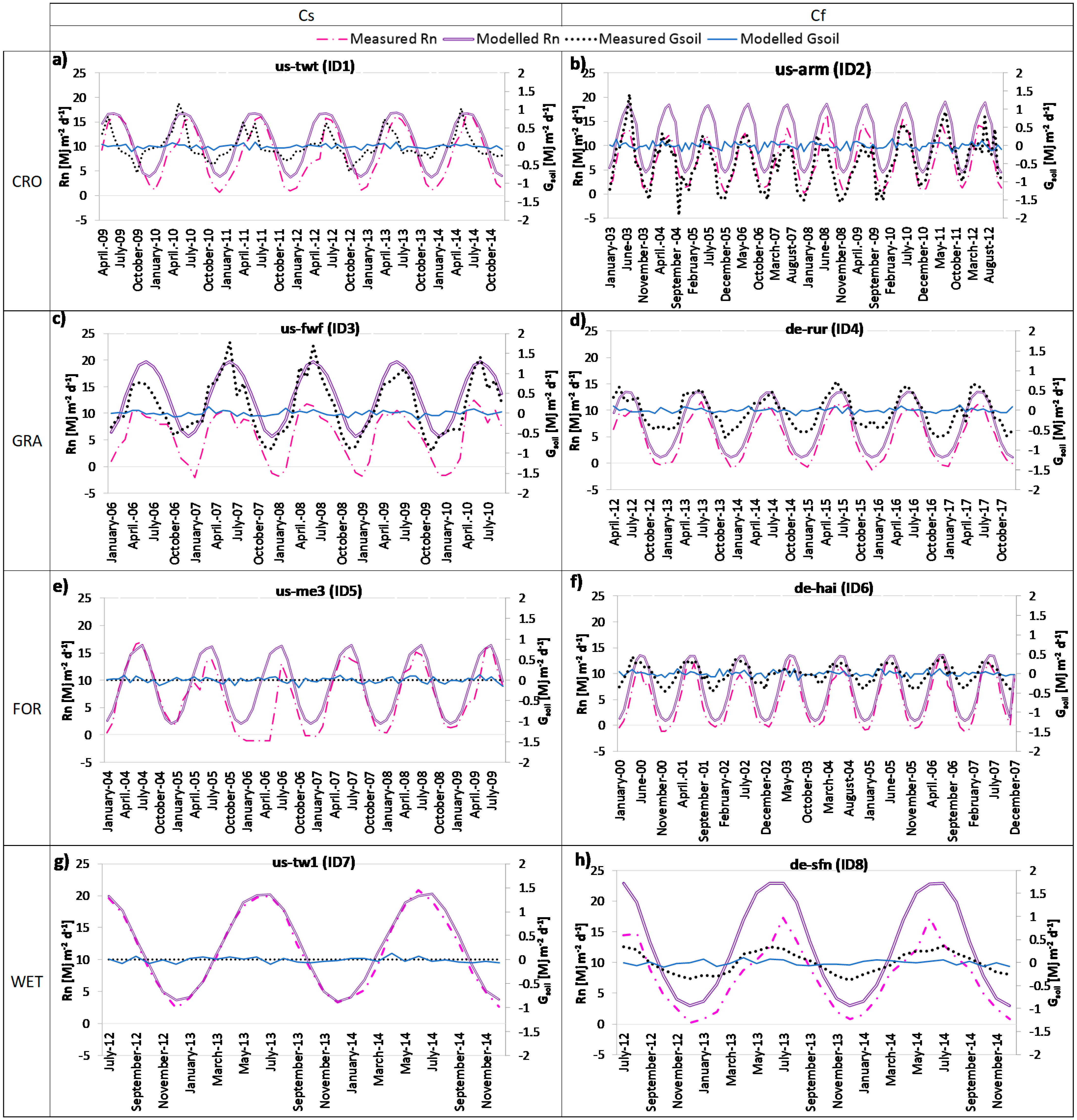
The use of modelled fluxes also impacts on the choice of the most performing method. For the site ID4 the most effective approach changes from API model to AA model with the use of empirically derived variables while for the site ID8, the AA model gives way to GG model (Table 5). The empirical formula used in case of lack of measured data to compute the net radiation overestimates the observed Rn values reaching RMSE at most of 1.31 (ID3) while the equation used for the computation of Gsoil strongly underestimates the measurements with values of RMSE even lower than −45 as it can be deduced from Table 6.

In confirmation of what stated above, Figure 5 reveals that even if the measured and simulated values of net radiation have similar temporal dynamics, they differ in terms of magnitude. On the other side, the predicted soil heat-flux density values strongly differ from the observed ones both in term of size and temporal development. Indeed, the observed Gsoil follows a seasonal pattern with growing phases from March to October and peak values approximately on July, the decreasing phases occur during Autumn and Winter with lowest values during October and November. The modelled soil heat flux follows a temporal pattern where there is no chance to identify a seasonality not even identifiable peaks but the curve appears almost flattened.

Since all models considerably overestimate the observed ET, a calibration procedure appears essential to reduce the prediction errors.

Ref. [38] came to the same conclusion, indeed, it considered the calibration an essential procedure to adapt the application of ET models to the regional conditions.

In the same way, ref. [42] found large biases when ET models are applied in inappropriate regimes in which the considered approach has been not developed.

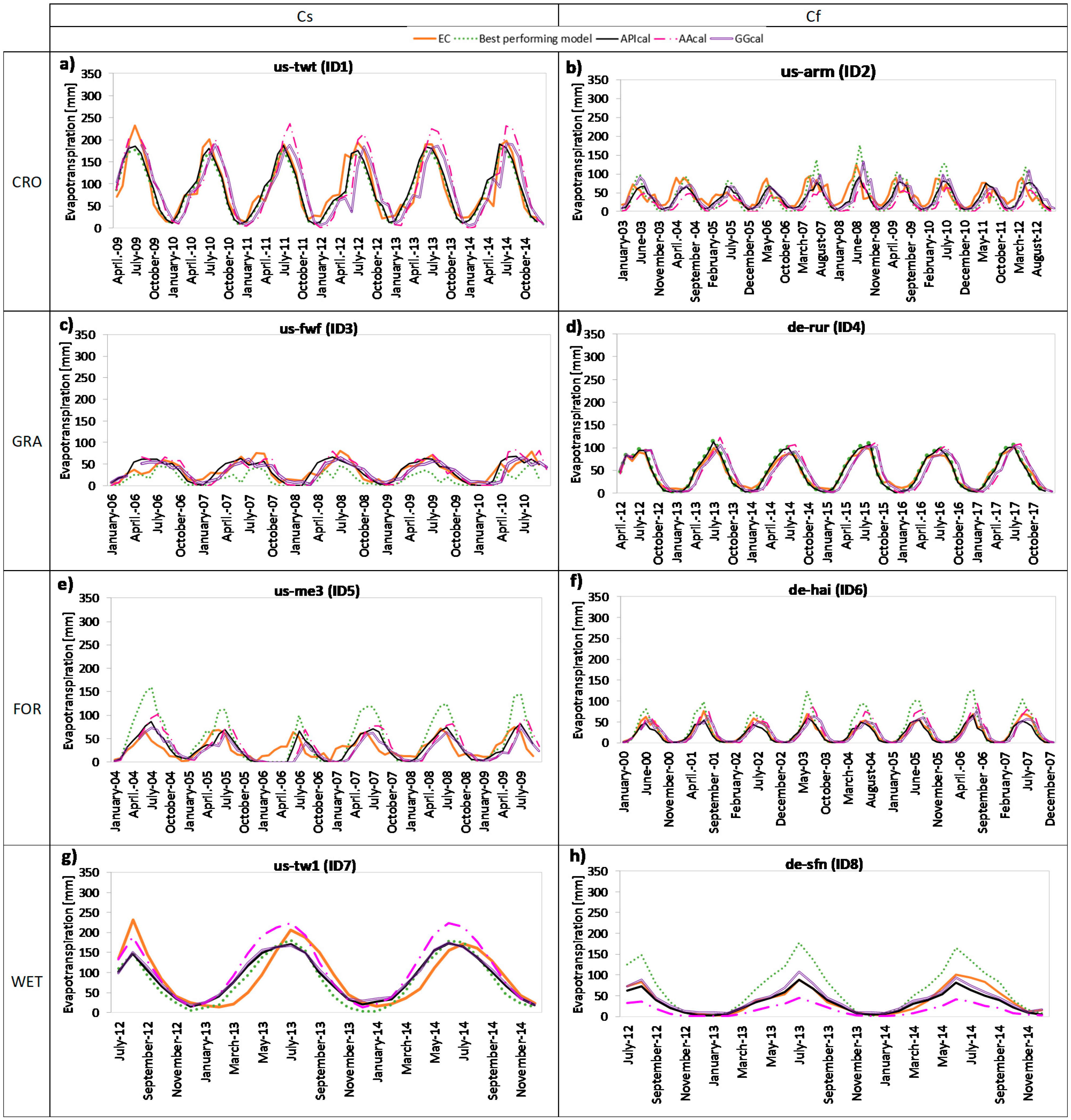
In the present study, when the monthly patterns of ET losses modelled using the calibrated approaches are compared with the ET resulting from the best performing models before the calibration process, the former results more consistent with the ET fluxes provided by the eddy-covariance towers (Figure 6)

This is confirmed by the values of the errors (Table 7) which also highlight that the site-specific calibration allows to increase the accuracy in ET predictions of the API, AA, and GG approaches. In details, GG_cal model seems to be the most accurate model in case of calibration, while AA_cal is the worst performing approach probably due to the complex calibration process in two-step.

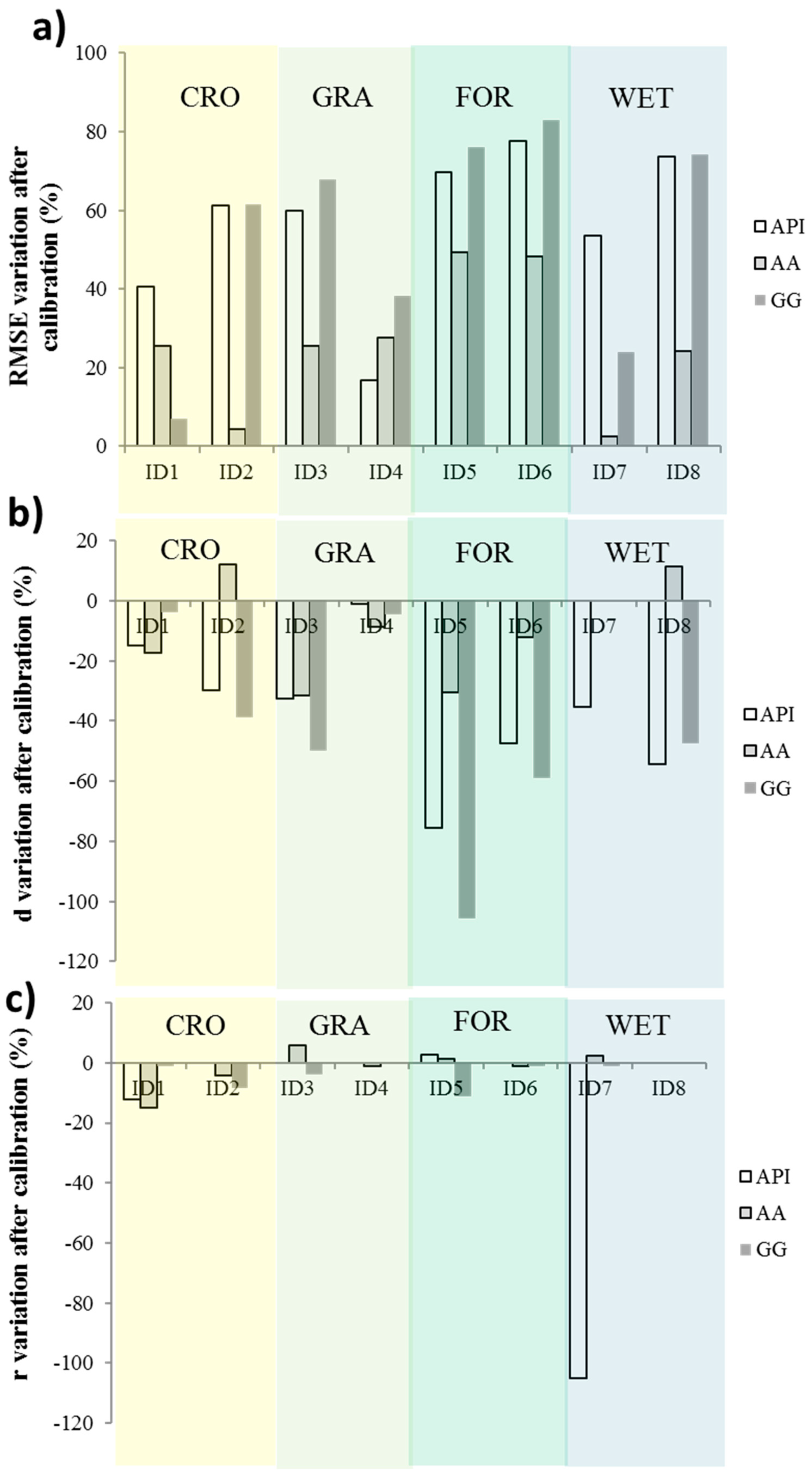
In Figure 7, the improvement related to the calibration procedure can be detected with greater clarity indeed, the variations in the values of RMSE, d, and r before and after the calibration process are shown. The relative difference in RMSE before and after the calibration process is overall positive which implies that the error decreases due to this procedure and consequently, the model performance increases for each site and approach. In the same way, the variations of r and d are overall negative, so the calibration process allows to improve these indices which results in an increasing model performance for each site and approach. The relative differences in the values of RMSE and d are considerably higher than the differences in r, with peaks for FOR vegetation type. Among the considered models, the GG approach resulting the best performing calibrated method, is the most impacted by the calibration procedure, indeed, it returns variation of RMSE up to 83% and reduction of d up to 106%.

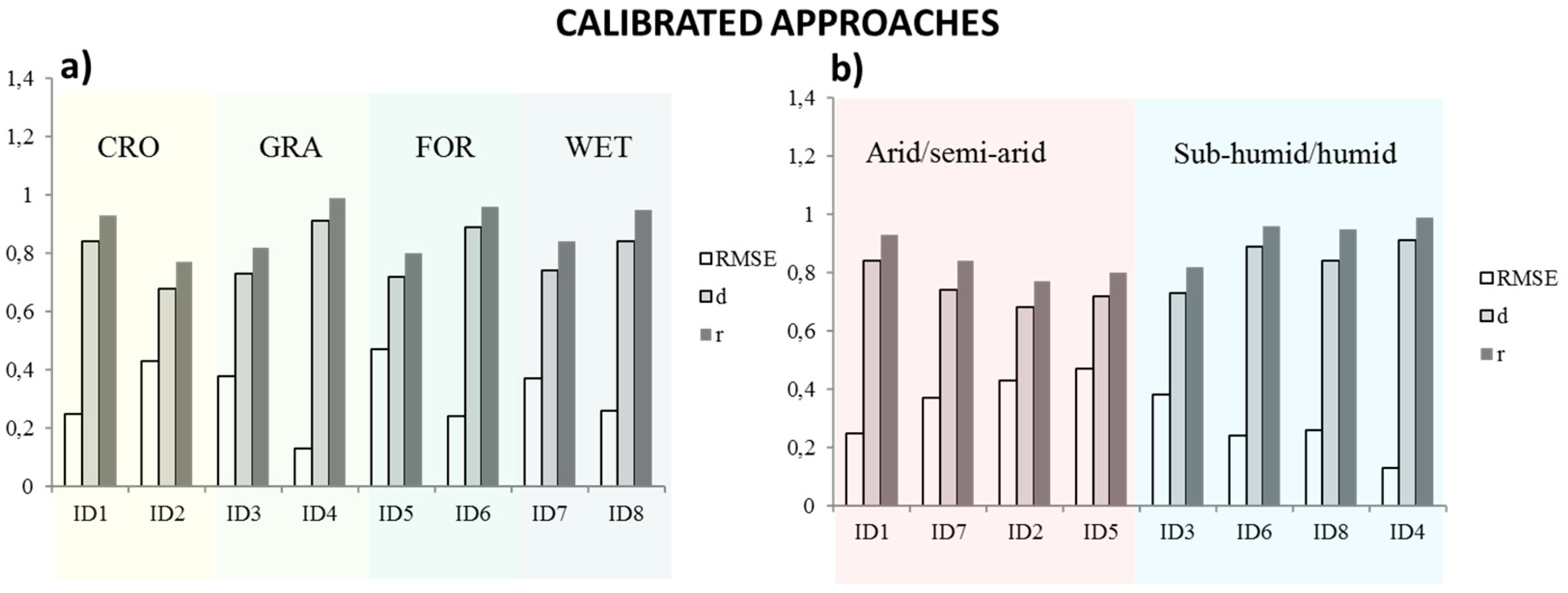
For what concerns the performances of the calibrated models with regard to the climate conditions and the vegetation type, it can be said that the sites with sub-humid/humid climates (Cfb) as in the case of non-calibrated approaches, present the best fitting (Figure 8 right panel) while the systems with forest land cover are associated with the largest prediction errors (Figure 8 left panel).

5. Conclusions

The performances of six meteorological data-based models in the prediction of ET have been investigated using high-quality datasets from eight eddy covariance towers belonging to TERENO, FLUXNET, and AMERIFLUX networks. The eight sites are characterized by different climates and vegetation types. In each of the considered sites, the AET losses have been predicted at monthly scale, using the GG, the AA, and the API approaches while the PET fluxes have been modelled using BC, PT, and PM methods belonging respectively to the categories of temperature-based, radiation-based, and combination-based approaches. It is difficult to detect a general accuracy of the approaches which depends on the characteristics of the site, and to identify a single model able to outperform the others for a considered biome but some general tendencies appear.

The AET models are better able to predict the ET fluxes than the PET approaches. Before the calibration process, the AA method is the best performing in almost each system. The sites characterized by arid/semi-arid climates and forest vegetation type present the largest average model errors with values around 64% for RMSE, 68% for d, and 87% for r. The poor performances of the selected approaches in arid region could be related to the evapotranspiration controlling factor that is the soil moisture rather than the climate variables and to the predominantly humid background conditions in which the models were developed. The low accuracy linked to the forest systems is presumably due to the roughness sub-layer effect which could influence eddy covariance measurements and to the heterogeneous land surfaces which could produce errors in the input data.

The low predictive power of the ET models in some biomes confirms the need for a site-specific calibration procedure which allows to obtain better model accuracy. For the AA model, the parameters involved in the calibration process are the wind function f(u) and the α-coefficient, the parameters subject to calibration are the relative evaporation G and the α-coefficient respectively for GG model and API method. The calibration process of AA model consists of two phases, so it is particularly complex and the parameters resulting from this procedure significantly differ from their original values.

The calibration process allows to improve the models accuracy resulting in average values of RMSE, d, and r respectively close to 32%, 80%, and 88%. Even after the calibration, the sites with arid/semi-arid climates and forest vegetation type are associated to the lowest model accuracy. The most accurate model becomes GG method after the calibration procedure, at the same time, it results the most affected by this process while the least impacted is the AA models. In addition, the model errors in case of use of empirical formulas to derive Rn and Gsoil have been calculated. Indeed, if the measured data of these variables are not available at the experimental site, they can be indirectly estimated from climate data. The results suggest that the errors values increase with a consequent reduction of the model accuracy. Despite the worsening of the performances, in some cases of lack of measurements, the use of empirical formulas and so of an approach fully based on meteorological data is the only way forward. The model calibration has been only performed assuming that the variables Rn and Gsoil were available from in situ measurements. Indeed, the use of empirical formulas to derive net radiation and soil heat-flux would have caused a larger models distortion during the calibration phase and consequently higher estimation errors.

When, in an experimental site, the only measured variables are precipitation and temperature as it happens in most of the local weather stations, the best choice to model ET fluxes is the use of API model. Indeed, this approach requires as input parameters only precipitation, Rn and Gsoil which can be indirectly derived from the temperature. The other models proposed in the present work also require for their implementation, the wind speed and air humidity which, contrary to Rn and Gsoil, cannot be empirically estimated from temperature. Finally, the results of the present comparative study in contrasting environment have provided suggestions and recommendations for the selection of the best suited methodology to be used for ET predictions both in case of calibration/ non-calibrated procedures and in case of lack of measured data.

References

1. Trajkovic, S. Temperature-based approaches for estimating reference evapotranspiration. J. Irrig. Drain. Eng. 2005, 131, 316–323. [Google Scholar] [CrossRef]
2. Sartor, J.; Mobilia, M.; Longobardi, A. Results and findings from 15 years of sustainable urban storm water management. Int. J. Saf. Secur. Eng. 2018, 8, 505–514. [Google Scholar] [CrossRef]
3. Mobilia, M.; Longobardi, A. Model details, parametrization, and accuracy in daily scale green roof hydrological conceptual simulation. Atmosphere 2020, 11, 575. [Google Scholar] [CrossRef]
4. Abbaspour, K.C.; Rouholahnejad, E.; Vaghefi, S.; Srinivasan, R.; Yang, H.; Kløved, B. A continental-scale hydrology and water quality model for Europe: Calibration and uncertainty of a high-resolution large-scale SWAT model. J. Hydrol. 2015, 524, 733–752. [Google Scholar] [CrossRef] [Green Version]
5. Fortuniak, K.; Pawlak, W.; Bednorz, L.; Grygoruk, M.; Siedlecki, M.; Zieliński, M. Methane and carbon dioxide fluxes of a temperate mire in Central Europe. Agric. For. Meteorol. 2017, 23, 306–318. [Google Scholar] [CrossRef]
6. McMahon, T.A.; Peel, M.C.; Lowe, L.; Srikanthan, R.; McVicar, T.R. Estimating actual, potential, reference crop and pan evaporation using standard meteorological data: A pragmatic synthesis. Hydrol. Earth Syst. Sci. 2013, 17, 1331–1363. [Google Scholar] [CrossRef] [Green Version]
7. Remesan, R.; Mathew, J. Data-based evapotranspiration modeling. In Hydrological Data Driven Modelling. Earth Systems Data and Models; Remesan, R., Mathew, J., Eds.; Springer: Cham, Switzerland, 2015; Volume 1, pp. 183–230. [Google Scholar]
8. Anayah, F.M.; Kaluarachchi, J.J. Improving the complementary methods to estimate evapotranspiration under diverse climatic and physical conditions. Hydrol. Earth Syst. Sci. 2014, 18, 2049. [Google Scholar] [CrossRef] [Green Version]
9. Martinez, C.J.; Thepadia, M. Estimating reference evapotranspiration with minimum data in Florida. J. Irrig. Drain. Eng. 2009, 136, 494–501. [Google Scholar] [CrossRef]
10. Valipour, M. Temperature analysis of reference evapotranspiration models. Meteorol. Appl. 2015, 22, 385–394. [Google Scholar] [CrossRef]
11. Xu, C.Y.; Singh, V.P. Cross comparison of empirical equations for calculating potential evapotranspiration with data from Switzerland. Water Resour. Manag. 2002, 16, 197–219. [Google Scholar]
12. Priestley, C.H.B.; Taylor, R.J. On the assessment of surface heat flux and evaporation using large-scale parameters. Mon. Weather Rev. 1972, 100, 81–92. [Google Scholar] [CrossRef]
13. Turc, L. Estimation of irrigation water requirements, potential evapotranspiration: A simple climatic formula evolved up to date. Ann. Agron. 1961, 12, 13–49. [Google Scholar]
14. Abtew, W. Evapotranspiration measurements and modeling for three wetland systems in south Florida. J. Am. Water Resour. Assoc. 1996, 32, 465–473. [Google Scholar] [CrossRef]
15. Hargreaves, G. Preciseness of estimated reference crop evapotranspiration. J. Irrig. Drain. Eng. 1989, 115, 1000–1007. [Google Scholar] [CrossRef]
16. Thornthwaite, C.W. An approach toward a rational classification of climate. Geogr. Rev. 1948, 38, 55–94. [Google Scholar] [CrossRef]
17. Blaney, H.F.; Criddle, W.D. Determining water requirements in irrigated areas from climatological and irrigation data. Soil Conserv. Serv. 1950, 96, 32–33. [Google Scholar]
18. Linacre, E.T. A simple formula for estimating evaporation rates in various climates, using temperature data alone. Agric. Meteorol. 1977, 18, 409–424. [Google Scholar] [CrossRef]
19. Monteith, J.L. Evaporation and Environment. Symp. Soc. Exp. Biol. 1965, 19, 205–234. [Google Scholar]
20. Fisher, J.B.; Whittaker, R.J.; Malhi, Y. ET come home: Potential evapotranspiration in geographical ecology. Global Ecol. Biogeogr. 2011, 20, 1–18. [Google Scholar] [CrossRef]
21. Mawdsley, J.A.; Ali, M.F. Estimating nonpotential evapotranspiration by means of the equilibrium evaporation concept. Water Resour. Res. 1985, 21, 383–391. [Google Scholar] [CrossRef]
22. Brutsaert, W. Hydrology: An Introduction; Cambridge University Press: Cambridge, UK, 2005. [Google Scholar]
23. Marasco, D.E.; Culligan, P.J.; McGillis, W.R. Evaluation of common evapotranspiration models based on measurements from two extensive green roofs in New York City. Ecol. Eng. 2015, 84, 451–462. [Google Scholar] [CrossRef] [Green Version]
24. Mobilia, M.; Schmidt, M.; Longobardi, A. Modelling actual evapotranspiration seasonal variability by meteorological data-based models. Hydrology 2020, 7, 50. [Google Scholar] [CrossRef]
25. Han, S.; Hu, H.; Yang, D. A complementary relationship evaporation model referring to the Granger model and the advection aridity model. Hydrol. Process. 2011, 25, 2094–2101. [Google Scholar] [CrossRef]
26. Brutsaert, W.; Stricker, H. An advection aridity approach to estimate actual regional evapotranspiration. Water Resour. Res. 1979, 15, 443–450. [Google Scholar] [CrossRef]
27. Yang, Y.; Su, H.; Zhang, R.; Xia, J. Revised advection-aridity evaporation model. J. Hydrol. Eng. 2012, 18, 655–664. [Google Scholar] [CrossRef]
28. Mobilia, M.; Longobardi, A.; Sartor, J.F. Including a-priori assessment of actual evapotranspiration for green roof daily scale hydrological modelling. Water 2017, 9, 72. [Google Scholar] [CrossRef] [Green Version]
29. Granger, R.J.; Gray, D.M. Evaporation from natural nonsaturated surfaces. J. Hydrol. 1989, 111, 21–29. [Google Scholar] [CrossRef]
30. Armstrong, R.N.; Pomeroy, J.W.; Martz, L.W. Estimating evaporation in a prairie landscape under drought conditions. Can. Water Resour. J. 2010, 35, 173–186. [Google Scholar] [CrossRef] [Green Version]
31. Xu, Z.X.; Li, J.Y. Estimating basin evapotranspiration using distributed hydrologic model. J. Hydrol. Eng. 2003, 8, 74–80. [Google Scholar] [CrossRef]
32. Szilagyi, J.; Hobbins, M.T.; Jozsa, J. Modified advection-aridity model of evapotranspiration. J. Hydrol. Eng. 2009, 14, 569–574. [Google Scholar] [CrossRef] [Green Version]
33. Temesgen, B.; Eching, S.; Davidoff, B.; Frame, K. Comparison of some reference evapotranspiration equations for California. J. Irrig. Drain. Eng. 2005, 131, 73–84. [Google Scholar] [CrossRef]
34. Ha, W.; Kolb, T.E.; Springer, A.E.; Dore, S.; O’Donnell, F.C.; Martinez Morales, R.; Lopez, S.M.; Koch, G.W. Evapotranspiration comparisons between eddy covariance measurements and meteorological and remote-sensing-based models in disturbed ponderosa pine forests. Ecohydrology 2015, 8, 1335–1350. [Google Scholar] [CrossRef]
35. Liu, G.; Liu, Y.; Hafeez, M.; Xu, D.; Vote, C. Comparison of two methods to derive time series of actual evapotranspiration using eddy covariance measurements in the southeastern Australia. J. Hydrol. 2012, 454, 1–6. [Google Scholar] [CrossRef]
36. Mobilia, M.; Longobardi, A. Evaluation of meteorological data-based models for potential and actual evapotranspiration losses using flux measurements. In Computational Science and Its Applications; Gervasi, O., Murgante, B., Misra, S., Garau, C., Blečić, I., Taniar, D., Apduhan, B.O., Rocha, A.M.A.C., Tarantino, E., Torre, C.M., et al., Eds.; Springer: Cham, Switzerland, 2020; Volume 12253. [Google Scholar]
37. Ershadi, A.; McCabe, M.F.; Evans, J.P.; Chaney, N.W.; Wood, E.F. Multi-site evaluation of terrestrial evaporation models using FLUXNET data. Agric. For. Meteorol. 2014, 187, 46–61. [Google Scholar] [CrossRef]
38. Bogawski, P.; Bednorz, E. Comparison and validation of selected evapotranspiration models for conditions in Poland (Central Europe). Water Resour. Manag. 2014, 28, 5021–5038. [Google Scholar] [CrossRef] [Green Version]
39. Lu, J.; Sun, G.; McNulty, S.G.; Amatya, D.M. A comparison of six potential evapotranspiration methods for regional use in the southeastern United States. J. Am. Water Resour. Assoc. 2005, 41, 621–633. [Google Scholar] [CrossRef]
40. Alkaeed, O.; Flores, C.; Jinno, K.; Tsutsumi, A. Comparison of several reference evapotranspiration methods for Itoshima Peninsula area, Fukuoka, Japan. Mem. Fac. Eng. 2006, 66, 1–14. [Google Scholar]
41. Fisher, J.B.; Tu, K.P.; Baldocchi, D.D. Global estimates of the land-atmosphere waterflux based on monthly AVHRR and ISLSCP-II data, validated at 16 FLUXNET sites. Remote Sens. Environ. 2008, 112, 901–919. [Google Scholar] [CrossRef]
42. Allen, R.G.; Pereira, L.S.; Raes, D.; Smith, M. Crop evapotranspiration. Guidelines for computing crop water requirements. FAO Irrig. Drain. 1999, 56, 1–50. [Google Scholar]
43. Xystrakis, F.; Matzarakis, A. Evaluation of 13 empirical reference potential evapotranspiration equations on the island of Crete in southern Greece. J. Irrig. Drain. 2011, 137, 211–222. [Google Scholar] [CrossRef] [Green Version]
44. Todorovic, M.; Karic, B.; Pereira, L.S. Reference evapotranspiration estimate with limited weather data across a range of Mediterranean climates. J. Hydrol. 2013, 481, 166–176. [Google Scholar] [CrossRef] [Green Version]
45. Suttie, J.M.; Reynolds, S.G.; Batello, C. Grasslands of the World; Food & Agriculture Org.: Rome, Italy, 2005; Volume 34. [Google Scholar]
46. NASA Earth Observatory. Available online: https://earthobservatory.nasa.gov/features/ForestCarbon (accessed on 23 March 2021).
47. Wu, W.; Yu, Q.; You, L.; Chen, K.; Tang, H.; Liu, J. Global cropping intensity gaps: Increasing food production without cropland expansion. Land Use Policy 2018, 76, 515–525. [Google Scholar] [CrossRef]
48. Mitsch, W.J.; Gosselink, J.G.; Zhang, L.; Anderson, C.J. Wetland Ecosystems; John Wiley & Sons: Hoboken, NJ, USA, 2009. [Google Scholar]
49. Knox, S.H.; Matthes, J.H.; Sturtevant, C.; Oikawa, P.Y.; Verfaillie, J.; Baldocchi, D. Biophysical controls on interannual variability in ecosystem-scale CO2 and CH4 exchange in a California rice paddy. J. Geophys. Res. Biogeosci. 2016, 121, 978–1001. [Google Scholar] [CrossRef]
50. Knox, S.; Matthes, J.H.; Verfaillie, J.; Baldocchi, D. FLUXNET2015 US-Twt Twitchell Island, Dataset; Fluxnet: Berkeley, CL, USA, 2009–2014. [Google Scholar] [CrossRef]
51. Sturtevant, C.; Ruddell, B.L.; Knox, S.H.; Verfaillie, J.; Matthes, J.H.; Oikawa, P.Y.; Baldocchi, D. Identifying scale-emergent, nonlinear, asynchronous processes of wetland methane exchange. J. Geophys. Res. Biogeosci. 2016, 121, 188–204. [Google Scholar] [CrossRef] [Green Version]
52. Valach, A.; Szutu, D.; Eichelmann, E.; Knox, S.; Verfaillie, J.; Baldocchi, D. FLUXNET-CH4 US-Tw1 Twitchell Wetland West Pond, Dataset; Fluxnet: Berkeley, CL, USA, 2011–2018. [Google Scholar] [CrossRef]
53. Hemes, K.S.; Chamberlain, S.D.; Eichelmann, E.; Anthony, T.; Valach, A.; Kasak, K.; Szutu, D.; Verfaillie, J.; Silver, W.L.; Baldocchi, D.D. Assessing the carbon and climate benefit of restoring degraded agricultural peat soils to managed wetlands. Agric. For. Meteorol. 2019, 268, 202–214. [Google Scholar] [CrossRef]
54. Lokupitiya, E.; Denning, S.; Paustian, K.; Baker, I.; Schaefer, K.; Verma, S.; Meyers, T.; Bernacchi, C.J.; Suyker, A.; Fischer, M. Incorporation of crop phenology in Simple Biosphere Model (SiBcrop) to improve land-atmosphere carbon exchanges from croplands. Biogeoscience 2009, 6, 969–986. [Google Scholar] [CrossRef] [Green Version]
55. Biraud, S.; Fischer, M.; Chan, S.; Torn, M. FLUXNET2015 US-ARM ARM Southern Great Plains Site—Lamont, Dataset; Fluxnet: Berkeley, CA, USA, 2016; pp. 2003–2012. [Google Scholar] [CrossRef]
56. Dore, S.; Montes-Helu, M.; Hart, S.C.; Hungate, B.A.; Koch, G.W.; Moon, J.B.; Finkral, A.J.; Kolb, T.E. Recovery of ponderosa pine ecosystem carbon and water fluxes from thinning and stand-replacing fire. Glob. Chang. Biol. 2012, 18, 3171–3185. [Google Scholar] [CrossRef]
57. Dore, S.; Kolb, T. AmeriFlux US-Fwf Flagstaff—Wildfire, Dataset; Fluxnet: Berkeley, CA, USA, 2016; pp. 2006–2010. [Google Scholar] [CrossRef]
58. Gebler, S.; Hendricks Franssen, H.J.; Putz, T.; Post, H.; Schmidt, M.; Vereecken, H. Actual evapotranspiration and precipitation measured by lysimeters: A comparison with eddy covariance and tipping bucket. Hydrol. Earth Syst. Sci. 2015, 19, 2145–2161. [Google Scholar] [CrossRef] [Green Version]
59. Post, H.; Hendricks Franssen, H.J.; Graf, A.; Schmidt, M.; Vereecken, H. Uncertainty analysis of eddy covariance CO2 flux measurements for different EC tower distances using an extended two-tower approach. Biogeoscience 2015, 12, 1205–1221. [Google Scholar] [CrossRef] [Green Version]
60. Knohl, A.; Schulze, E.-D.; Kolle, O.; Buchmann, N. Large carbon uptake by an unmanaged 250-year-old deciduous forest in Central Germany. Agric. For. Meteorol. 2003, 118, 151–167. [Google Scholar] [CrossRef]
61. Knohl, A.; Tiedemann, F.; Kolle, O.; Schulze, E.D.; Kutsch, W.; Herbst, M.; Siebicke, L. FLUXNET2015 DE-Hai Hainich, Dataset; Fluxnet: Berkeley, CA, USA, 2016; pp. 2000–2012. [Google Scholar] [CrossRef]
62. Kutsch, W.L.; Persson, T.; Schrumpf, M.; Moyano, F.E.; Mund, M.; Andersson, S.; Schulze, E.D. Heterotrophic soil respiration and soil carbon dynamics in the deciduous Hainich forest obtained by three approaches. Biogeochemistry 2010, 100, 167–183. [Google Scholar] [CrossRef] [Green Version]
63. Hommeltenberg, J.; Schmid, H.P.; Drösler, M.; Werle, P. Can a bog drained for forestry be a stronger carbon sink than a natural bog forest? Biogeoscience 2014, 11, 3477–3493. [Google Scholar] [CrossRef] [Green Version]
64. Klatt, J.; Schmid, H.P.; Mauder, M.; Steinbrecher, R. FLUXNET2015 DE-SfN Schechenfilz Nord, Dataset; Fluxnet: Berkeley, CL, USA, 2016; pp. 2012–2014. [Google Scholar] [CrossRef]
65. Law, B. FLUXNET2015 US-Me3 Metolius-Second Young Aged Pine, Dataset; Fluxnet: Berkeley, CL, USA, 2016; pp. 2004–2009. [Google Scholar] [CrossRef]
66. Vickers, D.; Thomas, C.; Pettijohn, C.; Martin, J.G.; Law, B. Five years of carbon fluxes and inherent water-use efficiency at two semi-arid pine forests with different disturbance histories. Chem. Phys. Meteorol. 2012, 64, 17159. [Google Scholar] [CrossRef] [Green Version]
67. Kwon, H.; Law, B.E.; Thomas, C.K.; Johnson, B.G. The influence of hydrological variability on inherent water use efficiency in forests of contrasting composition, age, and precipitation regimes in the Pacific Northwest. Agric. For. Meteorol. 2018, 249, 488–500. [Google Scholar] [CrossRef]
68. Zitouna-Chebbi, R.; Prévot, L.; Chakhar, A.; Marniche-Ben Abdallah, M.; Jacob, F. Observing actual evapotranspiration from flux tower eddy covariance measurements within a hilly watershed: Case study of the Kamech site, Cap Bon Peninsula, Tunisia. Atmosphere 2018, 9, 68. [Google Scholar] [CrossRef] [Green Version]
69. Papale, D.; Reichstein, M.; Aubinet, M.; Canfora, E.; Bernhofer, C.; Kutsch, W.; Longdoz, B.; Rambal, S.; Valentini, R.; Vesala, T.; et al. Towards a standardized processing of net ecosystem exchange measured with eddy covariance technique: Algorithms and uncertainty estimation. Biogeoscience 2006, 3, 571–583. [Google Scholar] [CrossRef] [Green Version]
70. Reichstein, M.; Falge, E.; Baldocchi, D.; Papale, D.; Aubinet, M.; Berbigier, P.; Bernhofer, C.; Buchmann, N.; Gilmanov, T.; Granier, A.; et al. On the separation of net ecosystem exchange into assimilation and ecosystem respiration: Review and improved algorithm. Glob. Chang. Biol. 2005, 11, 1424–1439. [Google Scholar] [CrossRef]
71. Jensen, M.E.; Allen, R.G. Evaporation, Evapotranspiration, and Irrigation Water Requirements, 2nd ed.; ASCE: Reston, VA, USA, 2016. [Google Scholar]
72. Margonis, A.; Papaioannou, G.; Kerkides, P.; Bourazanis, G. Parameterization of “canopy resistance” and estimation of hourly latent heat flux over a crop. Eur. Water 2017, 59, 277–283. [Google Scholar]
73. Pereira, A.R.; Nova, N.A.V. Analysis of the Priestley-Taylor parameter. Agric. For. Meteorol. 1992, 61, 1–9. [Google Scholar] [CrossRef]
74. Eichinger, W.E.; Parlange, M.B.; Stricker, H. On the concept of equilibrium evaporation and the value of the Priestley-Taylor coefficient. Water Resour. Res. 1996, 32, 161–164. [Google Scholar] [CrossRef] [Green Version]
75. Sumner, D.M.; Jacobs, J.M. Utility of Penman-Monteith, Priestley-Taylor, reference evapotranspiration, and pan evaporation methods to estimate pasture evapotranspiration. J. Hydrol. 2005, 308, 81–104. [Google Scholar] [CrossRef]
76. Longobardi, A.; Khaertdinova, E. Relating soil moisture and air temperature to evapotranspiration fluxes during inter-storm periods at a Mediterranean experimental site. J. Arid Land 2015, 7, 27–36. [Google Scholar] [CrossRef] [Green Version]
77. Koehler, M.A.; Linsley, R.K. Predicting the Runoff from Storm Rainfall; Weather Bureau, Department of Commerce: Washington, DC, USA, 1951; Volume 34. [Google Scholar]
78. Tabari, H.; Grismer, M.E.; Trajkovic, S. Comparative analysis of 31 reference evapotranspiration methods under humid conditions. Irrig. Sci. 2013, 31, 107–117. [Google Scholar] [CrossRef]
79. Malek, E. Calibration of the Penman wind function using the Bowen ratio energy balance method. J. Hydrol. 1994, 163, 289–298. [Google Scholar] [CrossRef]
80. McNaughton, K.G.; Black, T.A. A study of evapotranspiration from a Douglas fir forest using the energy balance approach. Water Resour. Res. 1973, 9, 1579–1590. [Google Scholar] [CrossRef] [Green Version]
81. Cristea, N.C.; Kampf, S.K.; Burges, S.J. Revised coefficients for Priestley-Taylor and Makkink-Hansen equations for estimating daily reference evapotranspiration. J. Hydrol. Eng. 2013, 18, 1289–1300. [Google Scholar] [CrossRef] [Green Version]
82. Kohler, M.A.; Nordenson, T.J.; Fox, W.E. Evaporation from pans and lakes. Weather Bur. Res. 1955, 38, 1–20. [Google Scholar]
83. Hobbins, M.T.; Ramirez, J.A.; Brown, T.C. The complementary relationship in estimation of regional evapotranspiration: An enhanced advection-aridity model. Water Resour. Res. 2001, 37, 1389–1403. [Google Scholar] [CrossRef] [Green Version]
84. Kim, H.; Kaluarachchi, J.J. Estimating evapotranspiration using the complementary relationship and the Budyko framework. J. Water Clim. Chang. 2017, 8, 771–790. [Google Scholar] [CrossRef] [Green Version]
85. Long, D.; Singh, V.P. Integration of the GG model with SEBAL to produce time series of evapotranspiration of high spatial resolution at watershed scales. J. Geophys. Res. Atmos. 2001, 115, 1–22. [Google Scholar] [CrossRef] [Green Version]
86. Crago, R.D.; Qualls, R.J.; Feller, M. A calibrated advection-aridity evaporation model requiring no humidity data. Water Resour. Res. 2010, 46, 1–8. [Google Scholar] [CrossRef]
87. Crago, R.; Brutsaert, W. A comparison of several evaporation equations. Water Resour. Res. 1992, 28, 951–954. [Google Scholar] [CrossRef]
88. Crago, R.; Crowley, R. Complementary relationships for near-instantaneous evaporation. J. Hydrol. 2005, 300, 199–211. [Google Scholar] [CrossRef]
89. Weligepolage, K.; Gieske, A.S.M.; van der Tol, C.; Timmermans, J.; Su, Z. Effect of sub-layer corrections on the roughness parameterization of a Douglas fir forest. Agric. For. Meteorol. 2012, 162, 115–126. [Google Scholar] [CrossRef]
90. Harman, I.N. The role of roughness sublayer dynamics within surface exchange schemes. Bound.-Layer Meteorol. 2012, 142, 1–20. [Google Scholar] [CrossRef]
91. Xu, C.Y.; Singh, V.P. Evaluation of three complementary relationship evapotranspiration models by water balance approach to estimate actual regional evapotranspiration in different climatic regions. J. Hydrol. 2005, 308, 105–121. [Google Scholar] [CrossRef]
Figure 1. Location, Platform and identification number of the eddy covariance (EC) stations under investigation in (a) U.S.A. and (b) Europe.
Ijgi 10 00192 g001
Figure 2. Temporal patterns of the monthly average precipitation and air temperature for the eight selected sites: (a) us-twt, (b) us-arm, (c) us-fwf, (d) de-rur, (e) us-me3, (f) de-hai, (g) us-tw1, (h) de-sfn.
Ijgi 10 00192 g002
Figure 3. Temporal patterns of ET modelled using Antecedent Precipitation Index (API), Advection-Aridity (AA), Granger and Gray (GG), Penman-Monteith (PM), Priestley-Taylor (PT), Blaney–Criddle (BC) approaches and comparison with the measured fluxes for each of the selected site: (a) us-twt, (b) us-arm, (c) us-fwf, (d) de-rur, (e) us-me3, (f) de-hai, (g) us-tw1, (h) de-sfn.
Ijgi 10 00192 g003
Figure 4. Goodness-of-fit indices for the most accurate model and for all the sites in case of non-calibrated approaches. Reference is made to (a) land cover (CRO, GRA, FOR, WET that respectively stand for cropland, grassland, forest, and wetland) and to (b) the moisture index IM (arid/semi-arid versus sub-humid/humid, ID numbers are sorted for increasing IM).
Ijgi 10 00192 g004
Figure 5. Monthly patterns of observed and modelled Rn and Gsoil for each of the selected site: (a) us-twt, (b) us-arm, (c) us-fwf, (d) de-rur, (e) us-me3, (f) de-hai, (g) us-tw1, (h) de-sfn.
Ijgi 10 00192 g005
Figure 6. Monthly patterns of measured evapotranspiration fluxes and of modelled ones obtained by the calibrated models and by the most accurate non-calibrated approach for each of the selected site: (a) us-twt, (b) us-arm, (c) us-fwf, (d) de-rur, (e) us-me3, (f) de-hai, (g) us-tw1, (h) de-sfn.
Ijgi 10 00192 g006
Figure 7. Relative difference in (a) RMSE, (b) d, and (c) r before and after the calibration process.
Ijgi 10 00192 g007
Figure 8. Goodness-of-fit indices for the most accurate model and for all the sites in case of calibrated approaches. Reference is made to (a) land cover (CRO, GRA, FOR, WET that respectively stand for cropland, grassland, forest, and wetland) and to (b) the moisture index IM (arid/semi-arid versus sub-humid/humid, ID numbers are sorted for increasing IM).
Ijgi 10 00192 g008