Monitoring Vegetation Greenness in Response to Climate Variation along the Elevation Gradient in the Three-River Source Region of China

Abstract

The Three-River Source Region (TRSR) is vital to the ecological security of China. However, the impact of global warming on the dynamics of vegetation along the elevation gradient in the TRSR remains unclear. Accordingly, we used multi-source remote sensing vegetation indices (VIs) (GIMMS (Global Inventory Modeling and Mapping Studies) LAI (Leaf Area Index), GIMMS NDVI (Normalized Difference Vegetation Index), GLOBMAP (Global Mapping) LAI, MODIS (Moderate Resolution Imaging Spectroradiometer) EVI (Enhanced Vegetation Index), MODIS NDVI, and MODIS NIRv (near-infrared reflectance of vegetation)) and digital elevation model data to study the changes of VGEG (Vegetation Greenness along the Elevation Gradient) in the TRSR from 2001 to 2016. Results showed that the areas with a positive correlation of vegetation greenness and elevation accounted for 36.34 ± 5.82% of the study areas. The interannual variations of VGEG showed that the significantly changed regions were mainly observed in the elevation gradient of 4–5 km. The VGEG was strongest in the elevation gradient of 4–5 km and weakest in the elevation gradient of >5 km. Correlation analysis showed that the mean annual temperature was positively correlated with VIs, and the effect of the mean annual precipitation on VIs was more obvious at low altitude than in high altitude. This study contributes to our understanding of the VGEG variation in the TRSR under global climate variation and also helps in the prediction of future carbon cycle patterns.

1. Introduction

The accelerating global warming and CO₂ concentration have exerted widespread impacts on the terrestrial ecosystem since the 1980s [1,2,3]. The ecological consequences of global warming are likely to be more pronounced in high-mountain regions [4,5]. Increasing evidence shows that the rate of warming is amplified in mountain environments [6], which will cause divergent vegetation greenness along the elevation gradient (from low to high) [7]. Vegetation greenness along the elevation gradient (VGEG) can be defined as the trend (expressed by slope) of vegetation greenness along the elevation gradient to a certain extent. Generally, vegetation greenness decreases with the increased elevation due to the limitation of low temperature at high altitudes [8], which indicates a negative vegetation greenness along the elevation gradient. However, the elevation pattern of vegetation greenness is probably altered under global warming [5,9,10,11] because the warming rate of high-mountain regions is often greater than their low-elevation counterparts [4,12].

The Three River Source Region (TRSR) is located in the hinterland of the Qinghai-Tibet Plateau and is composed of mountainous landforms higher than 2000 m above sea level. The TRSR is also known as the “Water Tower of China” because it is the source of the Yellow River, the Yangtze River, and the Lantsang River. Approximately 40% of the world’s population is influenced by these rivers [13]. Grassland is the dominant vegetation type in the TRSR, playing essential roles in the carbon cycle [14,15,16], regional climate regulation [4], and ecological security [17]. As one of the regions with a sensitive and fragile ecological environment [18], the changes in climate and vegetation are critical to the ecological security of China and the countries in Southeastern Asia [19,20].

To date, there are increasing vegetation-elevation related studies in the alpine ecosystems of China. However, the existing studies drew diametrically opposing conclusions. Some studies pointed out that the greening rate of vegetation decreased at increasing elevation [8,21]. The opposite conclusions showed that vegetation greenness was increased along with an increasing elevation [22]. These studies have not reached a consensus on the dynamics of vegetation along the elevation gradient. One of the possible reasons is that the study periods do not match each other, and the conclusions of short-term research cannot be corroborated by long-term research. Another important reason may be the differences in research methods. These studies involved field investigation and remote sensing methods, the spatial scales of which are entirely different and probably led to different research results. The third possible reason is that these studies only used a single vegetation index (VI) for the study, which will inevitably introduce the uncertainty of the VI itself into the results. This uncertainty is probably derived from the photographic ability of the sensor, differences in noise processing methods, and so on. Therefore, it is urgent to use multi-source remote sensing observation data to recognize and measure uncertainty, which cannot be achieved by a single remote sensing data source.

The primary aims of this study are to test the hypothesis of whether the spatial pattern of VGEG has altered in the TRSR under climate variation and to obtain the uncertainty of VGEG. To achieve this goal, we first analyzed the spatial pattern of climate factors and their changes from 2001 to 2016 to understand the basic climate background in the TRSR better. After that, we used six remote sensing-based VIs and digital elevation model (DEM) data to explore the spatiotemporal changes in vegetation, the spatial pattern of VGEG, and its dynamics from 2001 to 2016. At last, we identified the main climate factors affecting vegetation greenness dynamics and their elevational distribution. The results of this study are expected to contribute to our understanding of the VGEG variation in the TRSR under the influences of global climate variation and also may help for the prediction of future carbon cycle patterns.

2. Materials and Methods

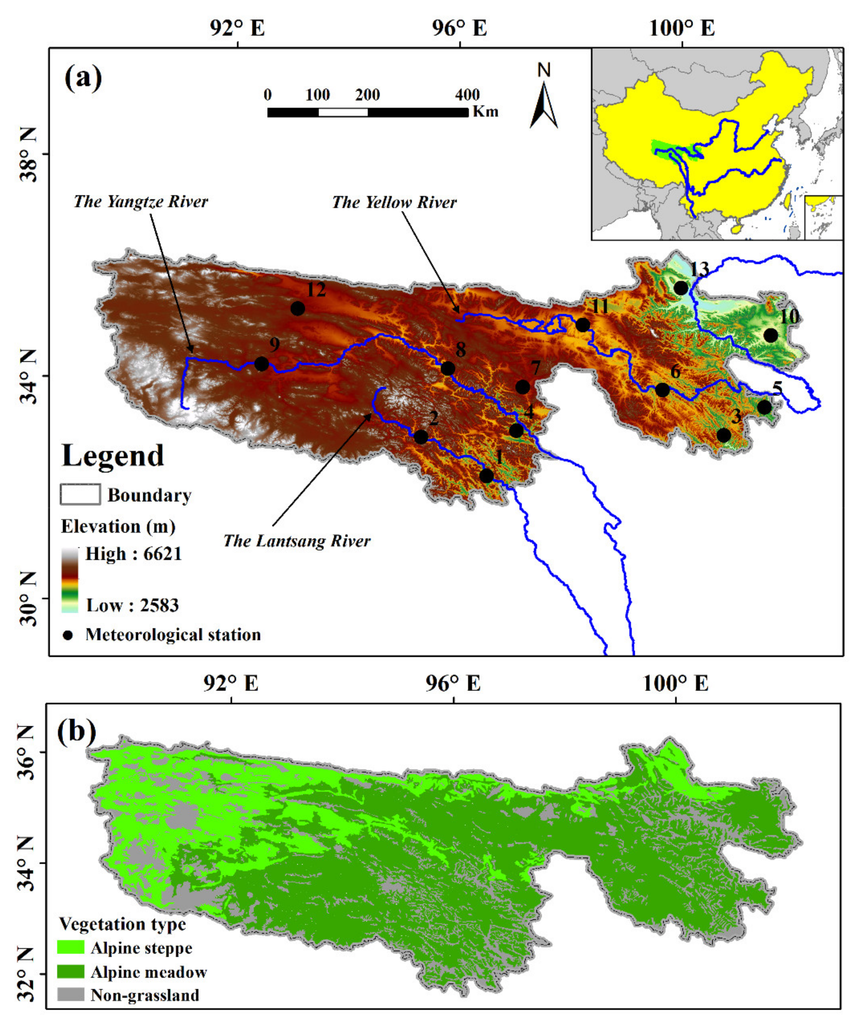
2.1. Study Area

The TRSR is located in western China (89.22–102.34° E, 31.01–37.13° N), covers more than 350,000 km² in area, and includes altitudes ranging from 2583 m to 6621 m (Figure 1). The TRSR is known as the “Water Tower of China”, which is essentially the headstream of the Yangtze River, the Yellow River, and the Lantsang River and supplies the water resource to approximately 40% of the world’s population [13]. Grassland is the primary ecosystem, covering approximately 80% of the total area, and the non-grassland land classification types were masked as gray. Alpine meadows (57%) and steppes (23%) are the dominant vegetation types in the TRSR [23]. The mean annual temperature (MAT) in the TRSR is generally from −5.6 °C to 7.8 °C, and the mean annual precipitation (MAP) is from 262.2 mm to 772.8 mm [24].

2.2. Remote Sensing Data

2.2.1. GIMMS NDVI

The third-generation Global Inventory Modeling and Mapping Studies (GIMMS) Normalized Difference Vegetation Index (NDVI), named the third generation NDVI dataset version 1 (GIMMS NDVI3g v1, hereinafter referred to as GIMMS NDVI), was adopted for vegetation trend analysis in many studies [25,26]. This dataset has a spatial resolution of 1/12° (≈9.2 km) and 15-day temporal frequency and improved the data quality in the high latitude compared with the previous version [27]. GIMMS NDVI was also used as the input data to generate GIMMS leaf area index (LAI) by the Feedforward Neural Network algorithm. Therefore, GIMMS NDVI shares the same temporal and spatial resolution with GIMMS LAI.

2.2.2. GIMMS LAI

The third-generation GIMMS LAI (LAI3g) (hereinafter referred to as GIMMS LAI) was generated by the Feedforward Neural Network (FFNN) algorithm, which was developed between the GIMMS NDVI and the best-quality Moderate Resolution Imaging Spectroradiometer (MODIS) LAI. On the spatial scale, GIMMS LAI data shares the same temporal and spatial resolution with GIMMS NDVI. We then resampled the GIMMS LAI data to the spatial resolution of 0.01° (≈1.1 km) by a cubic method consistent with the resolution of MODIS VI data. On the time scale, the maximum value composite method [28] was employed to merge the original 15-day data into annual data for analysis.

The FFNN is one of the widely used and rapidly developed artificial neural networks [29], and the neurons are arranged in layers. Each neuron is only connected to the neuron in the preceding layer. The network receives the output of the previous layer and outputs it to the next layer. No feedback occurred between the layers. In Zhu’s study, the FFNN models consisted of four neurons in the input layer (four input parameters corresponding to the land cover class, pixel-center latitude, pixel-center longitude, and NDVI3g), 11 neurons in the hidden layer, and 1 neuron in the output layer (LAI3g). MODIS LAI products for the overlapping period 2000–2009 were used in Zhu’s study [27]. The trained neural network algorithm was then used to generate the corresponding LAI.

The maximum value composite method is widely used to minimize negatively biased noise by selecting the highest VI value to represent a certain period (15 days in this study). Thus, the pixel with the highest VI value in the two 15-day VI represents the vegetation growth condition, and the average VI of 12-month was used to represent yearly data.

2.2.3. GLOBMAP LAI

Global Mapping (GLOBMAP) LAI version 3 dataset (1981–2016) at 8 km resolution was generated by the quantitative fusion of MODIS and historical Advanced Very High-Resolution Radiometer (AVHRR) data. MODIS LAI was generated from MODIS land surface reflectance data (MOD09A1) on the basis of the GLOBCARBON LAI algorithm [30]. The relationships between the AVHRR simple ratio and the MODIS LAI were established pixel by pixel by using two data series during the overlapped period (2000–2006). Then, the pixel-based relationship was used to estimate historical AVHRR LAI (1981–2000). Detailed descriptions and evaluation of the algorithm can be found in Liu’s article [31].

2.2.4. MODIS NDVI and EVI

We used the monthly VI product (MOD13A3, Collection 6) with a spatial resolution of 1 km to analyze the vegetation dynamics. The products include two primary VIs: the first one is the NDVI, and the second vegetation layer is the Enhanced VI (EVI).

NDVI, one of the widely used VIs, was constructed based on the spectral signature of vegetation, which has high reflectance in the near-infrared band and strong absorption in the red band. The EVI was developed to enhance the vegetation signal by reducing the influences of the canopy background signal and atmosphere [32]. MODIS EVI incorporates not only the red and near-infrared band but also the blue band to correct for aerosol influences in the red band and a soil adjustment factor to reduce the effect of canopy background. The EVI efficiently performed in heavy aerosol and biomass burning conditions. NDVI is likely to asymptotically saturate in high biomass regions, such as in the Amazon region; however, the EVI remained sensitive to canopy variations [32].

2.2.5. MODIS NIRv

The recently proposed near-infrared reflectance of vegetation (NIRv) is the product of total scene NIR reflectance and NDVI. NIRv is found to be strongly correlated with chlorophyll fluorescence and site-level gross primary productivity [33]. The temporal and spatial resolutions of NIRv are consistent with MODIS NDVI data.

In summary, the spatial resolution of all VI datasets was set to 0.01° (approximately equal to the original resolution of MODIS VI data). The study period of this work was set from 2001 to 2016 to maintain the consistency of the data on the time scale and facilitate the comparative research because MODIS VI data started in 2001, and GIMMS VI data only updated to 2016.

2.3. Meteorological Dataset

The raster meteorological datasets were derived from the National Tibetan Plateau Data Center (https://data.tpdc.ac.cn/en/ (accessed on 1 January 2021)). The original meteorological data of China, including the monthly temperature and precipitation data with a spatial resolution of 0.1° × 0.1°, covers the period 1979–2018 [34]. We further resampled the datasets to a spatial resolution of 0.01° × 0.01° by a cubic interpolation method and composite the monthly data to mean annual temperature (MAT) and precipitation (MAP) raster data, and then extracted the raster data of the TRSR from 2001 to 2016.

The site climatic data included average monthly temperature and precipitation data from 13 meteorological stations (numbered 1 to 13 in Figure 1) from 2001 to 2013, which were collected from the China Meteorological Data Sharing Service System (http://data.cma.cn/ (accessed on 1 January 2021)), as far as we could obtain. All of these stations are higher than 3300 m above sea level. The MAT of these stations ranged from −4.5 °C to 5.3 °C, and the MAP was from 342 mm to 728 mm. Eight out of 13 meteorological stations are located in alpine meadows, and five are located in alpine grasslands. The monthly climatic data of meteorological stations were composited to MAT and MAP to validate the raster MAT and MAP data from 2001 to 2013. The detailed characteristics of these meteorological stations are shown in

Table 1. The characteristics of the meteorological stations in the Three-River Source Region (TRSR).

No.	Latitude (°)	Longitude (°)	Elevation (m)	MAT (°C/y)	MAP (mm/y)	Vegetation Types
1	32.20000	96.48333	3629	5.3	573	Alpine meadow
2	32.90000	95.30000	4172	1.7	546	Alpine meadow
3	32.93333	100.75000	3663	3.5	643	Alpine meadow
4	33.01667	97.01667	3975	4.3	484	Alpine meadow
5	33.43333	101.48333	3626	1.6	728	Alpine meadow
6	33.75000	99.65000	3982	0.1	589	Alpine meadow
7	33.80000	97.13333	4426	−3.6	551	Alpine meadow
8	34.13333	95.78333	4194	−1.0	469	Alpine steppe
9	34.21667	92.43333	4536	−2.9	348	Alpine steppe
10	34.73333	101.60000	3519	0.4	605	Alpine meadow
11	34.91667	98.21667	4271	−2.6	359	Alpine steppe
12	35.21667	93.08333	4616	−4.5	342	Alpine steppe
13	35.58333	99.98333	3302	2.0	408	Alpine steppe

.

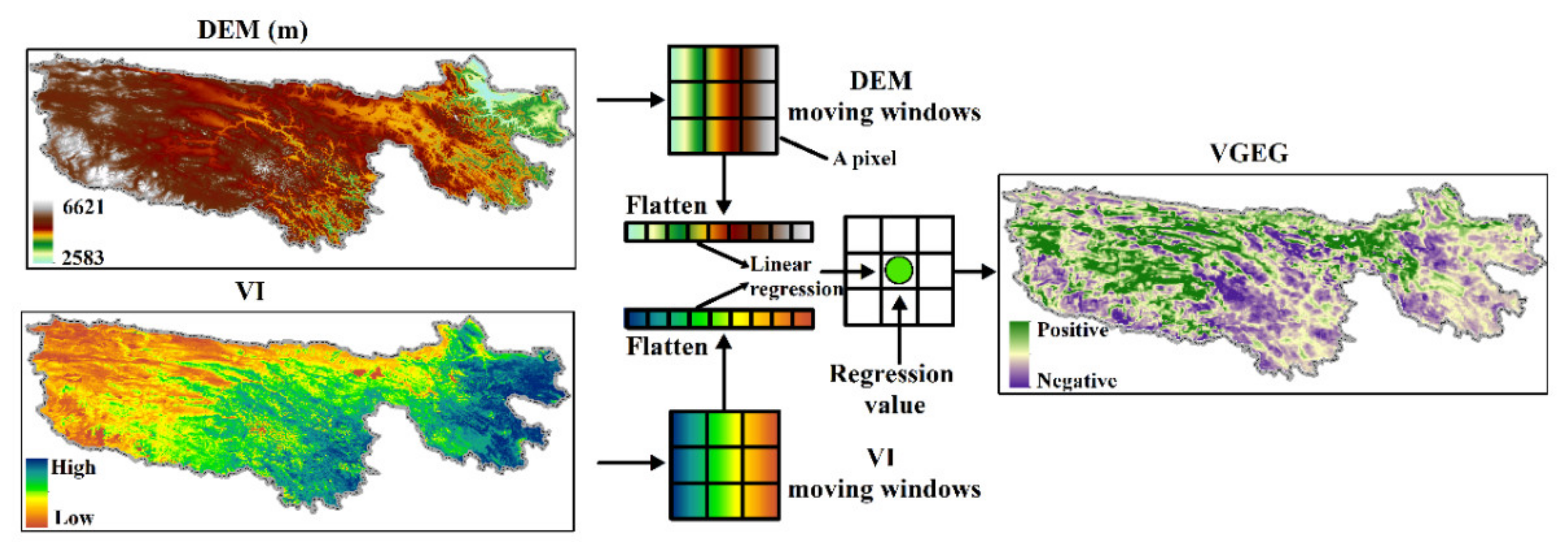
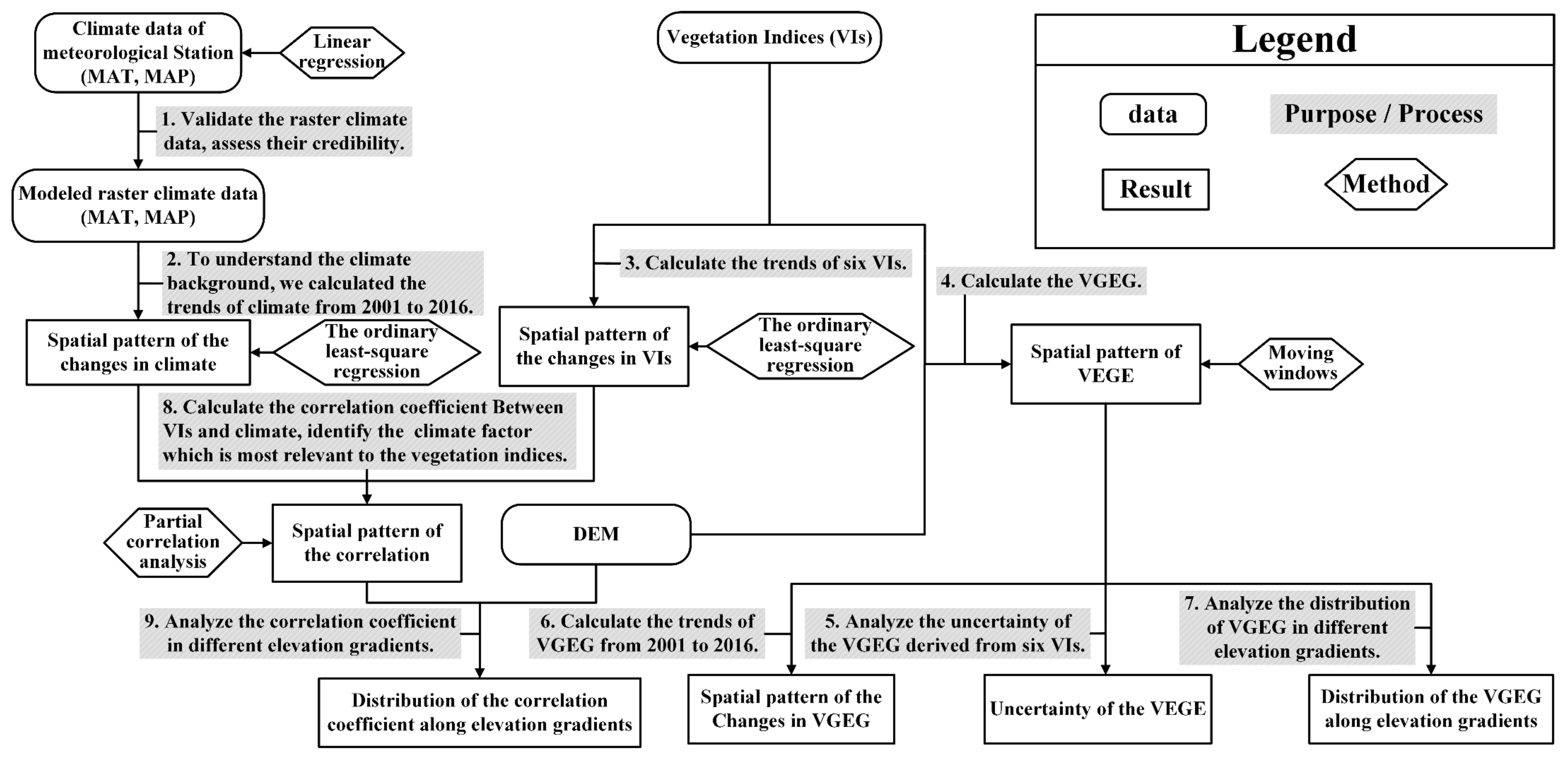
2.4. Calculation of the VGEG

VGEG can be defined as the trend (expressed by slope) of vegetation greenness along the elevation gradient to a certain extent (9 × 9 pixels in this study). The DEM data were obtained from the Shuttle Radar Topographic Mission with a spatial resolution of 30 m. The DEM data were resampled to a spatial resolution of 0.01° before any analysis. The linear regression slope analysis between the DEM and the VIs was performed in 9 × 9 moving windows (Figure 2). We obtained two groups of datasets, each containing 81 data values. The slope of the linear regression was signed to the center pixel of each 9 × 9 moving window. The significance of linear regression was tested by the T-test. The calculation process was executed by using Python 3.6.

2.5. Trend Analysis

We used the ordinary least-square regression method to determine the dynamics of the climate, VI, and VGEG over time series. The formula is described as follows:

$$\mathrm{Slope}=\frac{\mathrm{n}\times {{\displaystyle \sum }}_{\mathrm{i}=1}^{\mathrm{n}}{\mathrm{i}\times \left(\mathrm{VAR}\right)}_{\mathrm{i}}-\left({{\displaystyle \sum }}_{\mathrm{i}=1}^{\mathrm{n}}\mathrm{i}\right)\left({{\displaystyle \sum }}_{\mathrm{i}=1}^{\mathrm{n}}{\left(\mathrm{VAR}\right)}_{\mathrm{i}}\right)}{\mathrm{n}\times {{\displaystyle \sum }}_{\mathrm{i}=1}^{\mathrm{n}}{\mathrm{i}}^2-{\left({{\displaystyle \sum }}_{\mathrm{i}=1}^{\mathrm{n}}\mathrm{i}\right)}^2}$$

(1)

where VAR refers to MAT, MAP, each of the six VIs, and VGEG; i is the sequence number of the year (from 2001 to 2016), and n represents the total number of years. The significance of variables determined by the T-test represents the confidence level of variation.

2.6. Correlation Analysis

The correlation between VI and meteorological data (MAT and MAP) was analyzed using a partial correlation method from 2001 to 2016. The first step was to calculate the correlation coefficient (r) of the two variables in three variables (VI, MAT, and MAP) as Equation (2).

$${\mathrm{r}}_{\mathrm{xy}}=\frac{{{\displaystyle \sum }}_{\mathrm{i}=1}^{\mathrm{n}}\left({\mathrm{x}}_{\mathrm{i}}-\overline{\mathrm{x}}\right)\left({\mathrm{y}}_{\mathrm{i}}-\overline{\mathrm{y}}\right)}{\sqrt{{{\displaystyle \sum }}_{\mathrm{i}=1}^{\mathrm{n}}{\left({\mathrm{x}}_{\mathrm{i}}-\overline{\mathrm{x}}\right)}^2{{\displaystyle \sum }}_{\mathrm{i}=1}^{\mathrm{n}}{\left({\mathrm{y}}_{\mathrm{i}}-\overline{\mathrm{y}}\right)}^2}},$$

(2)

Three correlations were obtained, which were r₁₂, r₁₃, and r₂₃. Take the correlation coefficient between VI and temperature as an example. Variables x_i and y_i denote the VI and MAT in year i, respectively; $\overline{\mathrm{x}}$ and $\overline{\mathrm{y}}$ are the mean values of VI and MAT from 2001 to 2016, respectively. The partial correlations are calculated as follows:

$${\mathrm{r}}_{12, 3}=\frac{{\mathrm{r}}_{12}{-\mathrm{r}}_{13}{\mathrm{r}}_{23}}{\sqrt{{(1-\mathrm{r}}_{13}^2{\left)\right(\mathrm{r}–\mathrm{r}}_{23}^2)}}$$

(3)

$${\mathrm{r}}_{13, 2}=\frac{{\mathrm{r}}_{13}{-\mathrm{r}}_{12}{\mathrm{r}}_{23}}{\sqrt{{(1-\mathrm{r}}_{12}^2{\left)\right(\mathrm{r}-\mathrm{r}}_{23}^2)}}$$

(4)

$${\mathrm{r}}_{23, 1}=\frac{{\mathrm{r}}_{12}{-\mathrm{r}}_{13}{\mathrm{r}}_{23}}{\sqrt{{(1-\mathrm{r}}_{12}^2{\left)\right(\mathrm{r}-\mathrm{r}}_{13}^2)}}$$

(5)

We supposed that 1, 2, and 3 denote MAT, MAP, and VI, respectively. r₁₂, r₁₃, and r₂₃ indicate the correlation coefficients of MAT and MAP, MAT and VI, and MAP and VI, respectively. r_12,3 is the partial correlation coefficient of MAT and MAP, which removed the effect of VI. r_{13, 2}, and r_{23, 1} are the partial correlation coefficients of MAT and VI, MAP and VI, which removed the effect of MAP and MAT, respectively.

2.7. Data Processing and Analysis

The procedure of data processing and analysis in this study is shown in Figure 3. At first, we evaluated the credibility of raster climate data by using observed MAT and MAP from the meteorological stations. We calculated the trend of MAT and MAP to understand the dynamics of climate in the TRSR better. Then we investigated the spatial pattern of VI trends. After that, we combined VIs and DEM data to calculate the spatial pattern of VGEG. The changes in VGEG from 2001 to 2016 were also analyzed. In addition, we analyzed the distribution of VGEG in different elevation gradients. At last, we calculated the correlation coefficients between VIs and climate factors (MAT and MAP) and their elevational distribution to identify which climate factor had the highest correlation with the VIs at different altitude gradients.

3. Results

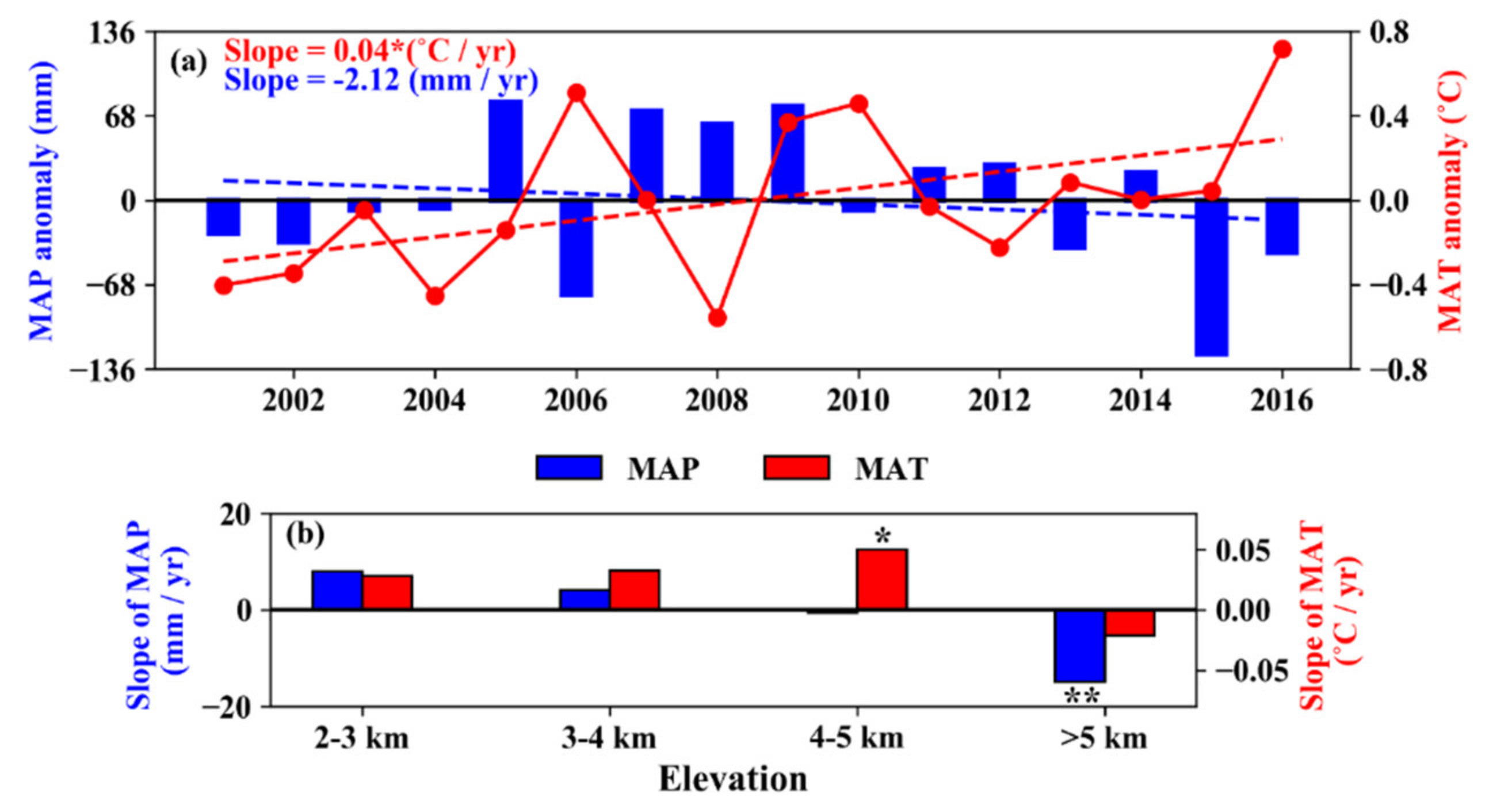
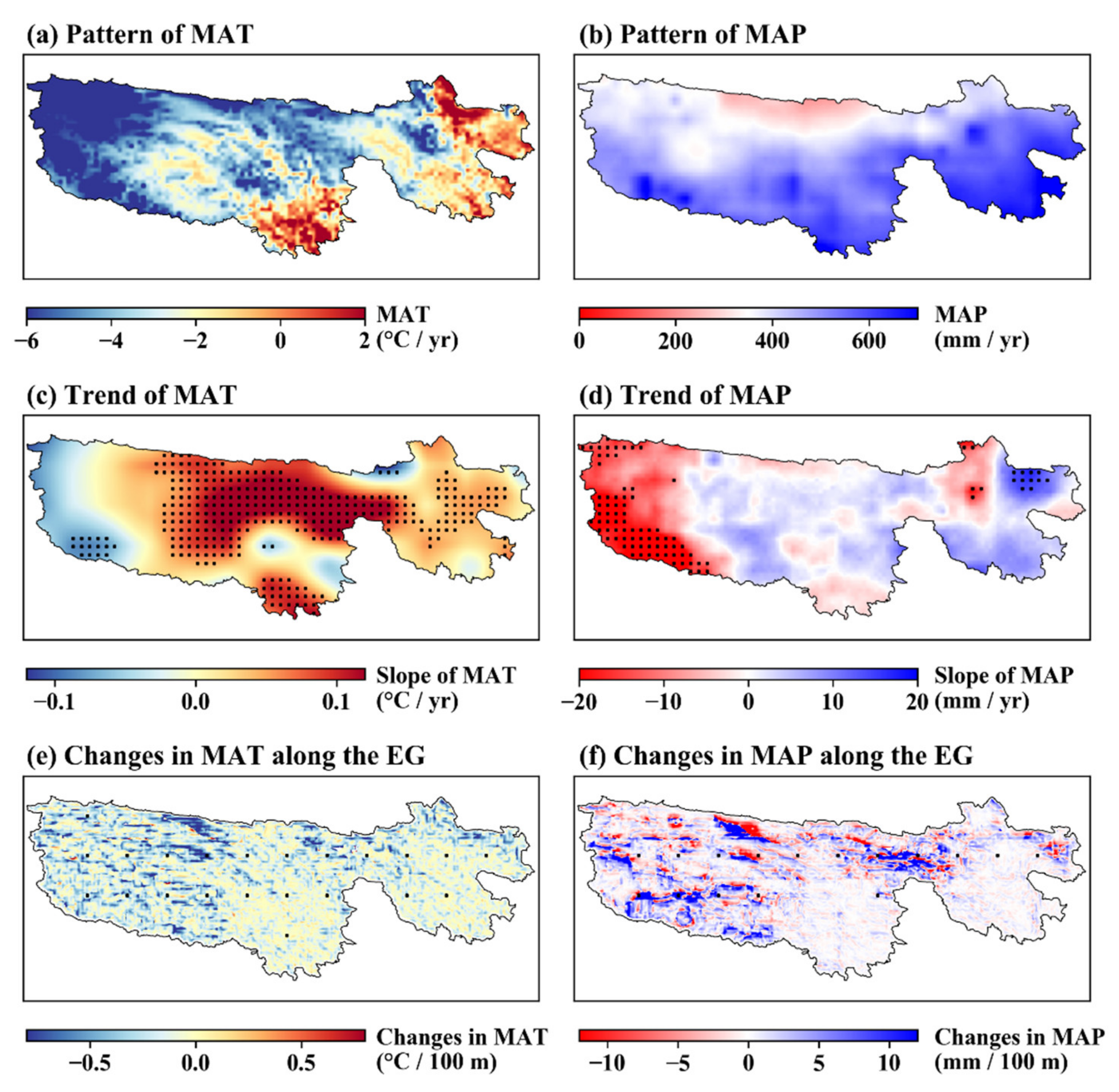
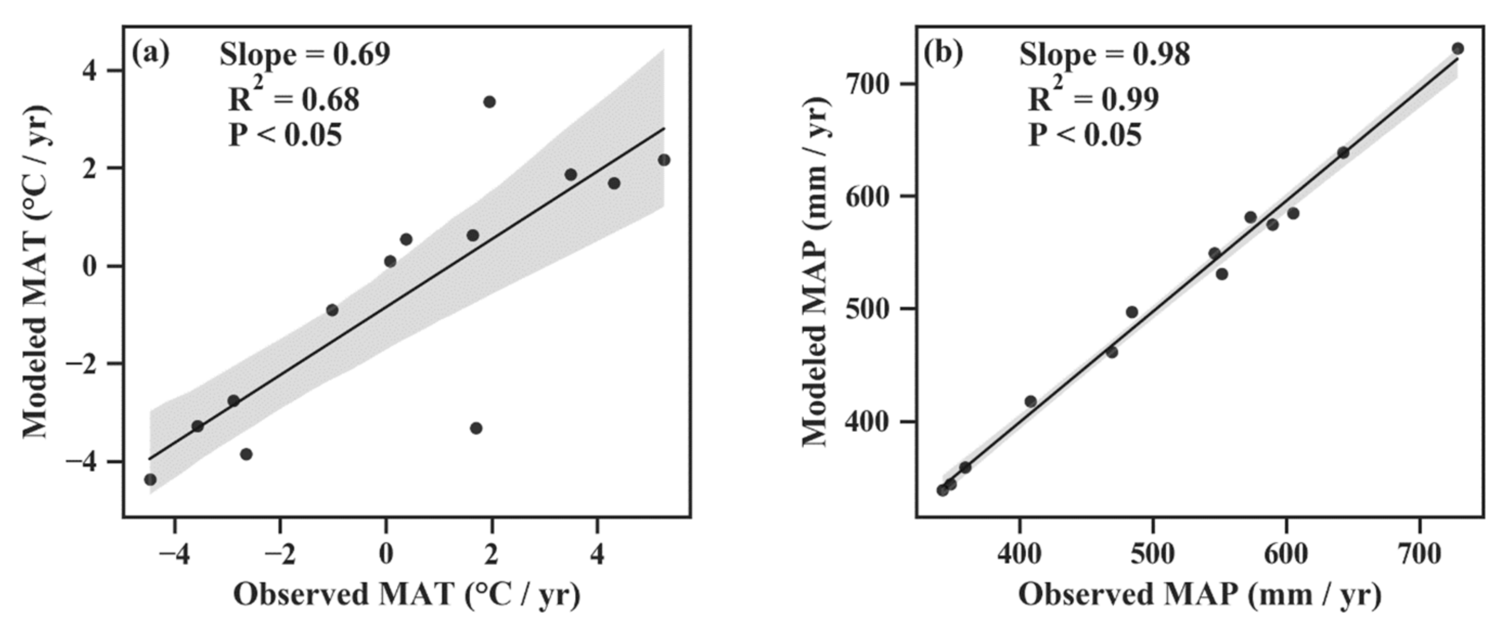
3.1. Validation and Trend of the Climate and Their Variation along Different Elevation

The MAT and MAP of the meteorological station (observed MAT and MAP) in 13 meteorological stations were used to validate the upscaled MAT and MAP raster data (Modeled MAT and MAP). The R² and slope of MAT were 0.68 and 0.69, respectively (Figure A1a). By contrast, the validation result of MAP was much better than that of MAT, and the R² and slope were 0.98 and 0.99, respectively (Figure A1b); these results were obtained maybe because the algorithm for precipitation is more complex than that for temperature as precipitation has high spatial heterogeneity [34]. In addition, the high R² and slope were mainly due to a large number of meteorological stations were used to generate the dataset. The validation result reached a significance level of 0.05.

In summary, the MAT increased at a rate of 0.04 °C/y in the TRSR from 2001 to 2016, and the increasing rate reached a significance level of 0.05 (Figure 4a). Meanwhile, precipitation was decreasing at a rate of 2.12 mm/y; however, the trend was not significant during the study period. The changes in the MAT and MAP along different elevation gradients are shown in (Figure 4b). The MAT increased in the elevation gradient (EG) of 2–3, 3–4, and 4–5 km, but it decreased in the EG of >5 km. The slope of 4–5 km reached a significance level of 0.05. The MAP exhibited a decreasing trend along the EGs. The slopes were positive in the EG of 2–3 and 3–4 km, whereas negative slopes were found in the EG of 4–5 and >5 km. The slope even reached a significance level of 0.01 in the EG of 4–5 km. In summary, the TRSR experienced significant warming from 2001 to 2016; however, the precipitation did not show a significant trend during the same period. The warming trend was significant in the EG of 4–5 km, whereas the precipitation was more pronounced in the EG of 2–3 and 3–4 km.

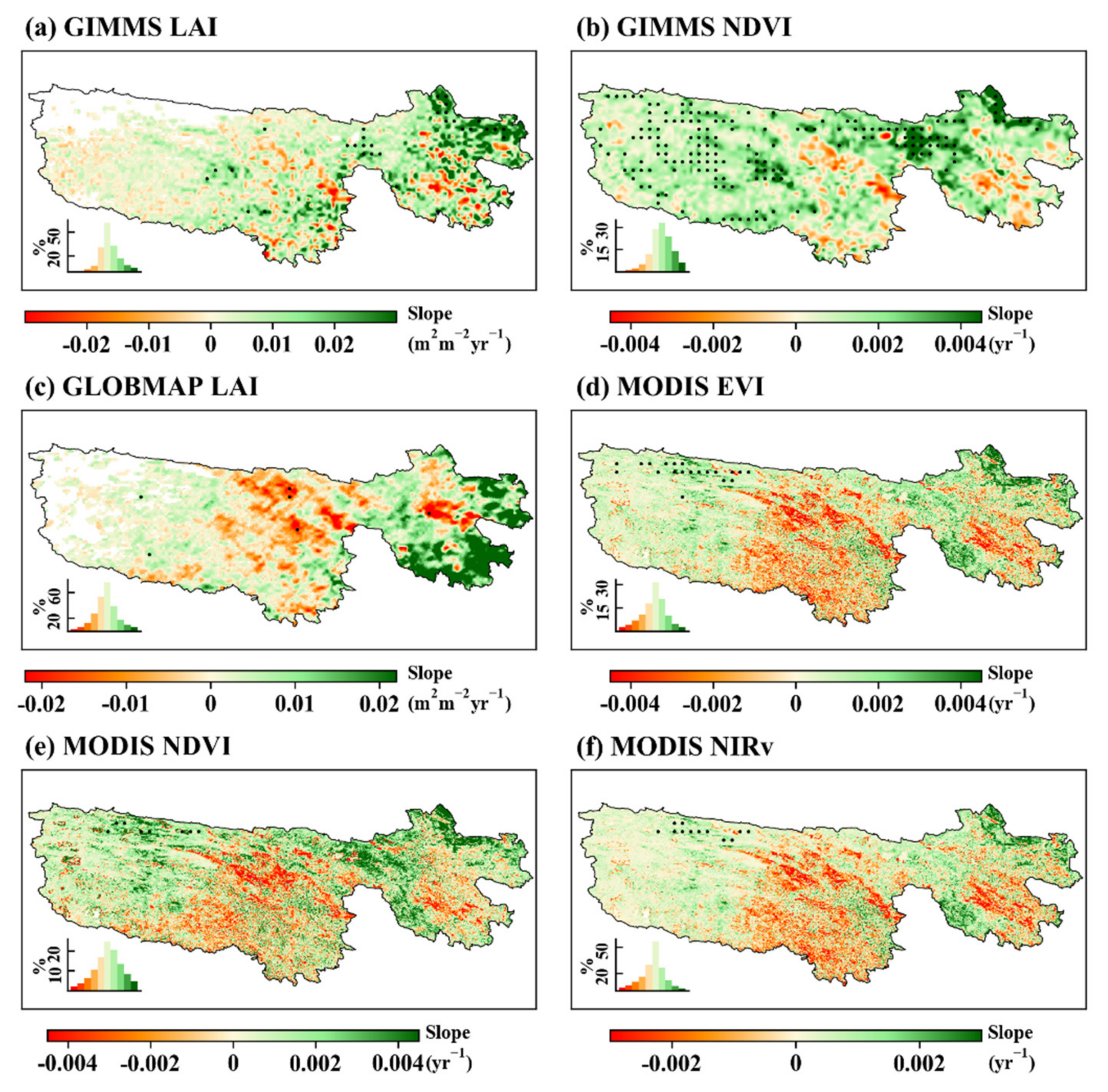
3.2. Spatial Patterns and Variations of the Climate and VIs

The spatial pattern of climate showed that the MAT was higher than −2 °C/y in the east and south of the TRSR, which was warmer than its west and north parts (Figure 5a). The MAP was over 400 mm/y in most parts of the TRSR and exhibited a decreasing trend from southeast to northwest (Figure 5b). We found that 76.30% of the study areas showed an increasing trend of MAT, and the MAT with a significant trend accounted for 40.71% (Figure 5c). By contrast, the regions with a negative trend of MAT only occupied 3.04% of the study areas, which were mainly found in the west of the TRSR. The areas with an increasing trend (52.25%) were slightly higher than that those with a decreasing trend (47.75%). However, the areas that reached a significant increasing trend only occupied 1.67%, which were mainly distributed in the eastern TRSR (Figure 5d). The regions with a significant decreasing trend accounted for 11.57%, which were found in the west of the TRSR. The spatial patterns of changes in MAT along elevation gradients from 2001 to 2016 are shown in Figure 5e. The positive changes in MAT were mainly found in the eastern TRSR and only accounted for 12.34% of the total study area; 4.64% reached a significant level of 0.05. The negative changes in MAT along elevation gradients were up to 87.66%, and 73.48% of the areas were statistically significant. The regions with positive changes in MAP were scattered across the western and central TRSR (Figure 5f). The areas accounted for 55.35% of the total study area, and 39.70% of the area reached a significant positive level. Approximately 44.65% of the area exhibited negative changes in MAP along elevation gradients, and the significant areas accounted for 30.04%.

The trend of VIs in the TRSR from 2001 to 2016 is shown in Figure 6. The VI exhibited an increasing trend in the TRSR (accounting for 68.06 ± 8.90% of the study areas), and 13.67 ± 8.90% of them reached a significance level of 0.05. The largest and least significant increasing areas were observed by GIMMS NDVI (28.72%) (Figure 6b) and MODIS NIRv (10.03%) (Figure 6f), respectively. By contrast, the areas with decreases in VI accounted for 31.94 ± 8.90% of the study areas, and only 2.43 ± 1.23% were statistically significant. The VIs did not significantly change in most study areas 83.90 ± 6.96%.

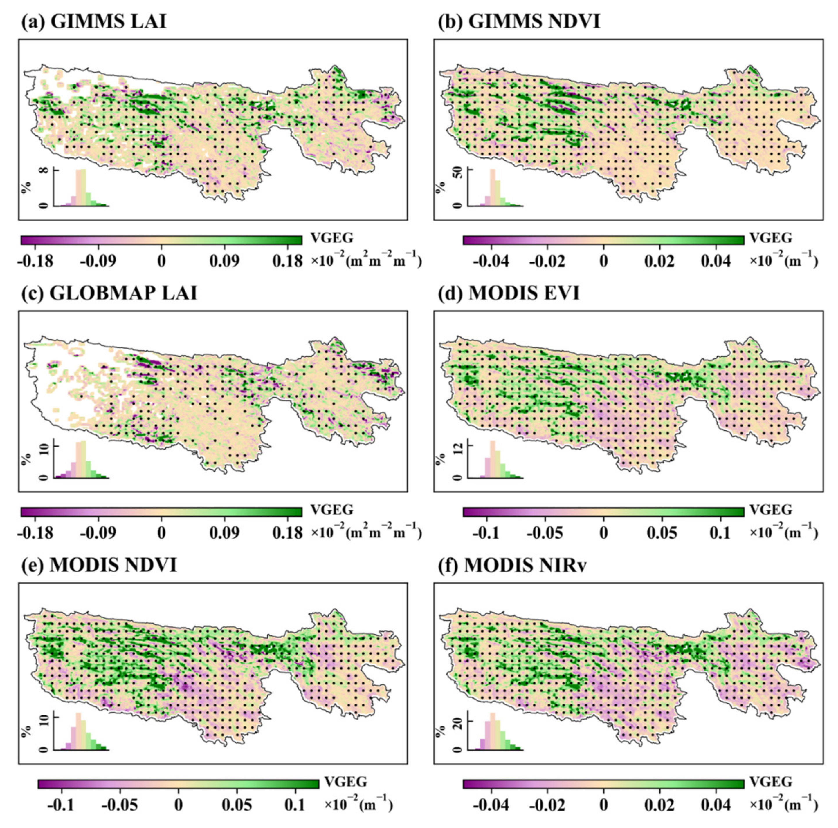
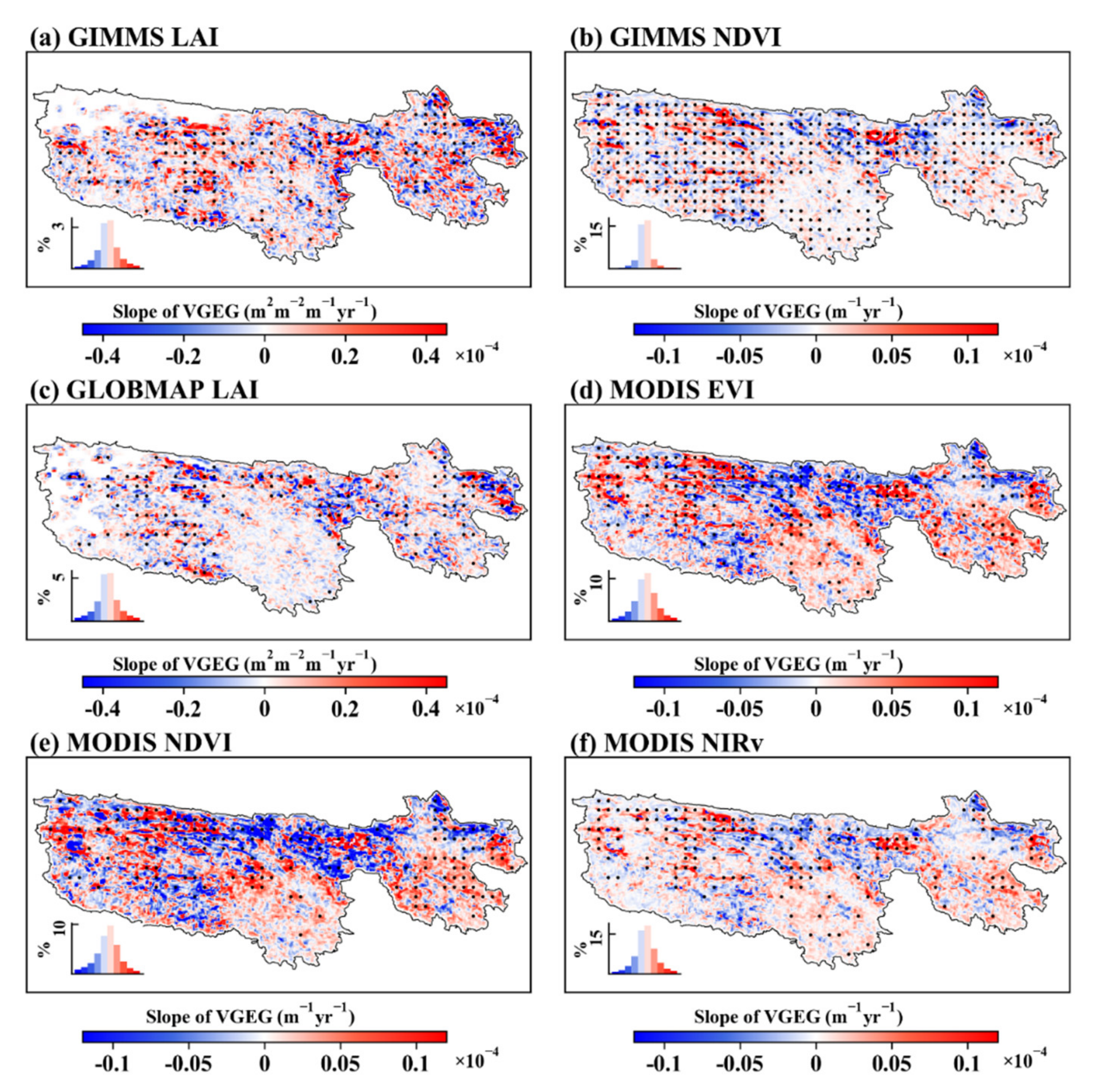
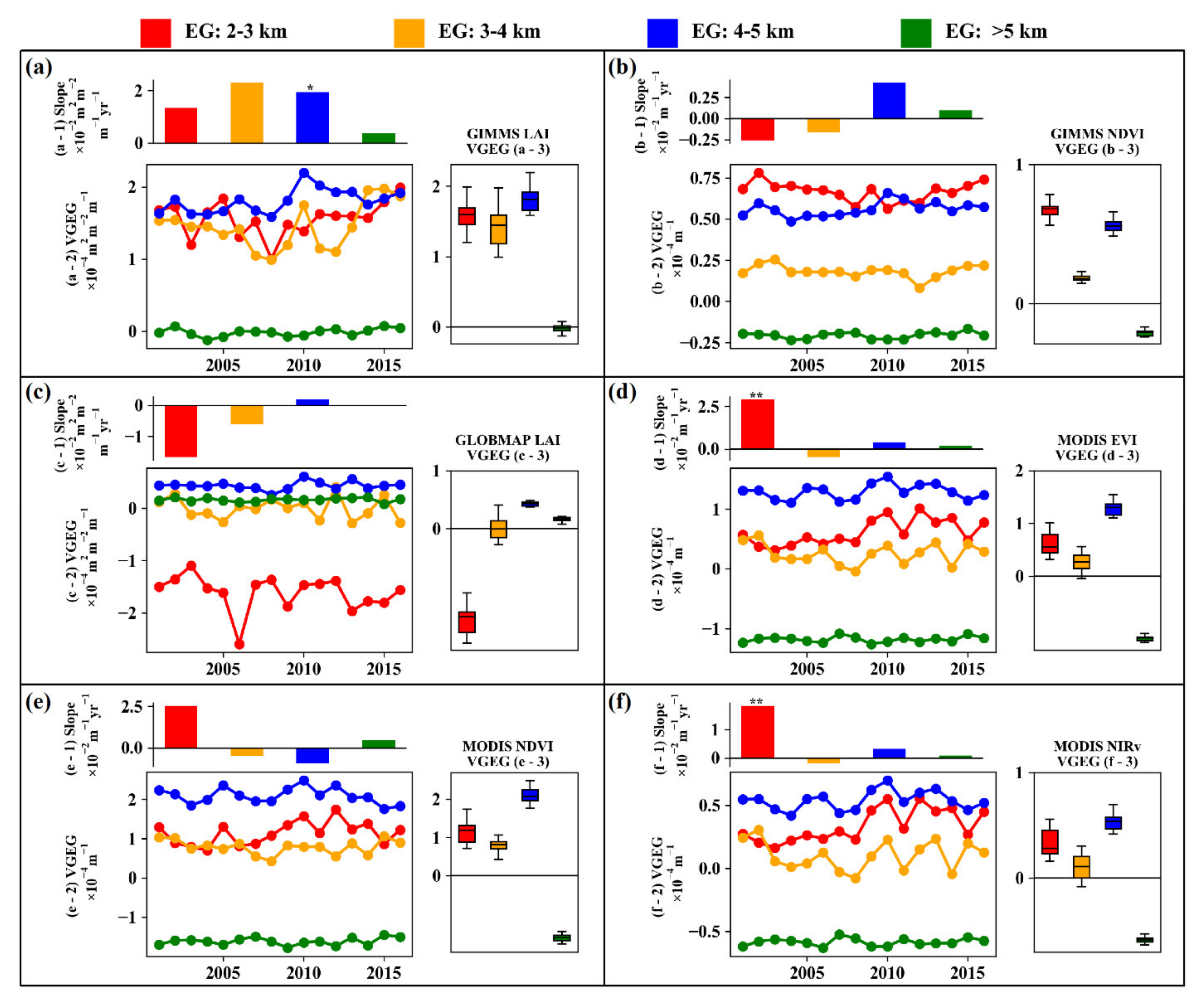
3.3. Spatial Patterns of the VGEG and Its Variations in Different Elevation

The spatial patterns of mean VGEG calculated by six types of VI from 2001 to 2016 are shown in Figure 7. The spatial patterns of VGEG had large differences between the GLOBMAP LAI and the other VIs (Figure 7c). The regions with negative VGEG were consistent with our perception that VI was decreased with increased elevation because of the lower temperature at higher altitudes. These regions were found in the center, southern, and eastern TRSR (Figure 7a,b,d–f), and the statistically significant negative areas accounted for 36.34 ± 5.82% of the study area. By contrast, the regions with positive VGEGs were mainly found in the western TRSR, and the areas of which were up to 37.23 ± 2.77% of the total study areas, thus indicating an increasing vegetation greenness along the elevation. The positive VGEG was likely induced by the homogenization of vegetation greenness from low attitude to its high-counterpart.

We calculated the VGEG of each year from 2001 to 2016, while the variations of VGEG showed strong spatial heterogeneity during the period (Figure 8). The VGEGs showed that the positive and negative trends accounted for 53.81% and 46.19% of the study areas, respectively. The significant positive trends of the VGEG accounted for 22.96 ± 3.31% of the study areas, which was greater than the regions with significant negative trends (20.73 ± 2.39%).

The regions that exhibited positive variation of VGEG were slightly higher than those with negative VGEG (53.45% vs. 46.56%), as observed by the six VIs from 2001 to 2016 (Figure 9). The statistically significant VGEG indicated that the regions with significant positive and negative VGEGs were mainly distributed in the elevation of 4–5 km and accounted for 43.62 ± 2.53% and 35.49 ± 2.55% of the study areas, respectively. By contrast, only less than 1% of the study areas that reached significant levels were distributed in the elevation of 2–3 km. The significant areas were no more than 10% at the elevation of 3–4 and 5–6 km. From the perspective of VGEG trends, the result of GIMMS LAI indicated that the VGEG trend was positive in four elevation gradients (2–3, 3–4, 4–5, and >5 km) from 2001 to 2016 (Figure 9(a-1)). The VGEG trend of GIMMS NDVI was similar to that of GLOBMAP LAI; that is, the trends were negative in 2–3, 3–4, and >5 km and positive in 4–5 km (Figure 9(b-1,c-1)). The VGEGs of MODIS EVI and MODIS NIRv had similar trends, which were positive in the elevation of 2–3, 4–5, and >5 km and negative at the elevation of 3–4 km. However, the VGEG trend of MODIS NDVI was negative at the elevation of 4–5 km (Figure 9(d-1,d-2,e-1,e-2,f-1,f-2)). The mean VGEG variations of GIMMS LAI, MODIS EVI, MODIS NDVI, and MODIS NIRv were strongest in the elevation of 4–5 km, followed by the elevations of 2–3, 3–4, and >5km (Figure 9(a-3,d-3,e-3,f-3)), which were completely different from the results of GIMMS NDVI and GLOBMAP LAI (Figure 9(b-3,c-3)).

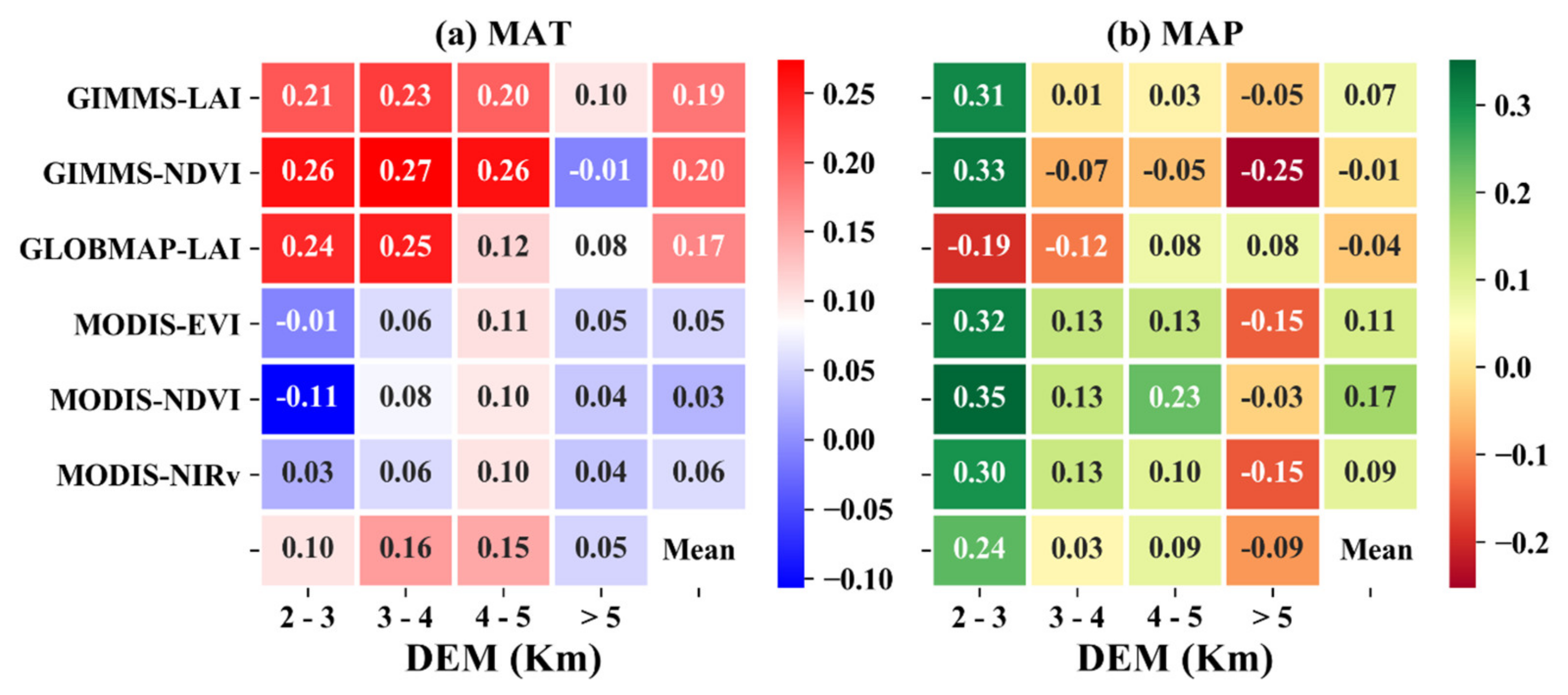
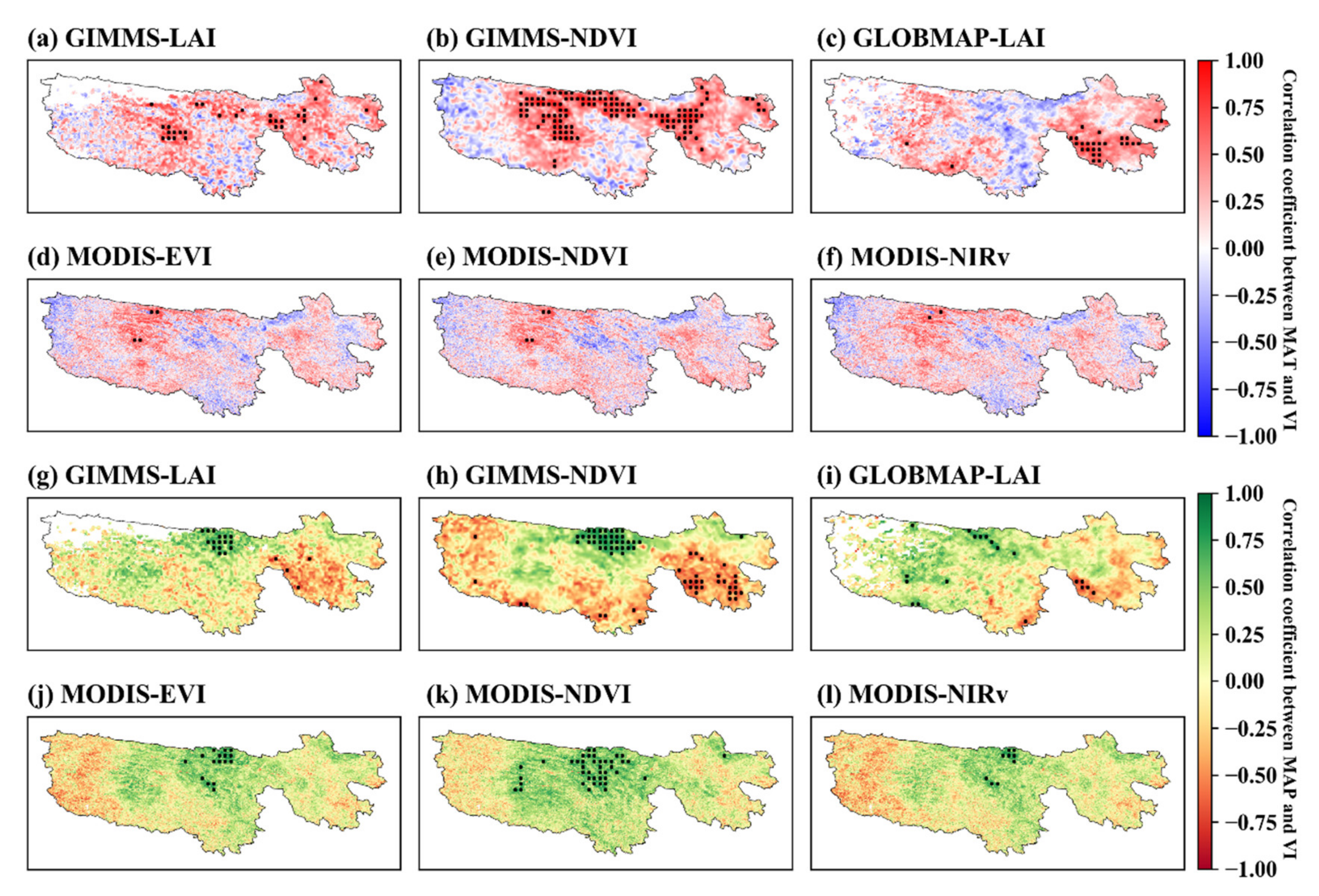
3.4. Correlation between VIs and Climatic Factors

The spatial patterns of the correlation between VIs and MAT have strong spatial heterogeneity (Figure A2). Most regions exhibited a positive correlation between VIs and MAT, which accounted for 65.15 ± 4.94% of the study areas, and 9.47 ± 4.83% of the areas reached a significance level of 0.05. The negative correlation between VIs and MAT accounted for 30.92 ± 5.84%, and no more than 2% of the areas reached a significant negative correlation.

We further analyzed the correlation between VIs and meteorological factors (MAT and MAP) in the elevation of 2–3, 3–4, 4–5, and >5 km from 2001 to 2016 (Figure 10). Most elevations exhibited a positive correlation of VIs and MAT (Figure 10a). The correlation of GIMMS and GLOBMAP-based VIs was higher than that of MODIS-based VIs. Meanwhile, the correlation of the elevation of 3–4 and 4–5 km was higher than that of 2–3 and >5 km. By contrast, the correlation between VIs and MAP was more complicated along the elevation gradient from 2001 to 2016 (Figure 10b). The positive correlations of MODIS-based VIs were higher than those of GIMMS and GLOBMAP-based VIs. The correlation between VIs and MAP was negative in the elevation of >5 km, and the VIs were positively correlated with MAP at low elevation. Furthermore, the correlation of VIs at low elevation was higher than that of VIs at high elevation. In summary, precipitation was the limiting factor for vegetation growth at the elevation of 2–3 km. However, the effect is likely to decrease with increasing elevation. The effect of temperature was even at every altitude gradient, except for the regions with an altitude > 5000 m above sea level.

In addition, we analyzed the dynamics of climate in the case of significant variations in the VIs from 2001 to 2016 (

Table 2. Dynamics of climate with the significant changes in vegetation indices (VIs).

VI	VI Trend 1	MAT			MAP
		Function	Cor 2	Sig 3.	Function	Cor 2	Sig 3.
GIMMS-LAI	+	VI = 2.374 * MAT − 5.424	0.73	0.001	VI = −29.16 * MAP + 526.9	−0.08	0.776
	−	VI = −0.8344 * MAT − 1.652	−0.31	0.246	VI = −65.04 * MAP + 641.2	−0.2	0.469
GIMMS-NDVI	+	VI = 13.91 * MAT − 8.338	0.54	0.03	VI = −974.6 * MAP + 714.8	−0.07	0.808
	−	VI = −1.533 * MAT − 2.764	−0.07	0.79	VI = −282.6 * MAP + 606.5	−0.08	0.782
GLOBMAP-LAI	+	VI = 1.95 * MAT − 5.492	0.52	0.037	VI = −134.2 * MAP + 611.8	−0.16	0.058
	−	VI = −2.231 * MAT − 7.744	−0.42	0.105	VI = 148.3 * MAP + 251.6	0.15	0.57
MODIS-EVI	+	VI = 8.515 * MAT − 6.431	0.21	0.433	VI = −1155 * MAP + 617.4	−0.17	0.526
	−	VI = −7.001 * MAT − 0.5537	0.15	0.57	VI = 302.5 * MAP + 380.6	0.1	0.7
MODIS-NDVI	+	VI = 6.045 * MAT − 6.397	0.30	0.262	VI = −142.8 * MAP + 462.4	0.04	0.874
	−	VI = −6.771 * MAT + 0.326	−0.48	0.06	VI = 582.4 * MAP + 181.5	0.27	0.31
MODIS-NIRv	+	VI = 1.95 * MAT − 5.492	0.22	0.411	VI = −2452 * MAP + 613.4	−0.22	0.419
	−	VI = −11.11 * MAT − 1.136	−0.42	0.102	VI = 344.6 * MAP + 428.1	0.06	0.838

¹ “+” and “−” denotes an increased and decreased trend of VI (vegetation index), respectively. ² Cor denotes the partial correlation of VI and climate (MAT: Mean Annual Temperature; MAP: Mean Annual Precipitation). ³ Sig. denotes the significance levels of the linear regression function between VI and climate.

). We used a linear regression method to represent clearly how climate dynamics with significant increasing VIs behaved. We can read that MAT increased with significant increases in VIs, and three of the six partial correlations of MAT and VIs (GIMMS LAI, GIMMS NDVI, and GLOBMAP LAI) reached a significance level of 0.05. Meanwhile, MAP was negatively correlated with the significant increasing trend of VIs; however, none of them passed the significance test. By contrast, MAT was likely to increase on the condition that VI exhibited a significant decreasing trend, and the partial correlation coefficients of MAT and VIs were negative. Meanwhile, MAP was positively correlated with four VIs (GLOBMAP LAI, MODIS EVI, MODIS NDVI, and MODIS NIRv) with significant negative trends and negatively correlated with the other two (GIMMS LAI and GIMMS NDVI). The partial correlations with VIs of either MAT or MAP did not reach a significant level.

In summary, the increases in VIs were positively correlated with MAT, and the partial correlation coefficients of three VIs and MAT had statistical significance. Precipitation was not the dominating climatic factor in the increases in VIs because precipitation decreased when VI increases. The decreases in VI were likely due to the increasing MAT and decreasing MAP (although two of the VIs were negatively correlated with MAP). However, we did not have enough evidence to prove this aspect, and certain partial correlation coefficients did not pass the significance test.

4. Discussion

4.1. Merit and Limitation

In this study, we used a moving window method to monitor the dynamics of vegetation greenness to climatic variation along elevation gradients. The size of the moving window limited the dynamics of vegetation greenness in a certain region, making it comparable in a relatively uniform climate. The moving window method also confirmed a theorem that the temperature decreases with the increase in altitude, which also proved that the method could effectively monitor the changes in variables along the elevation gradient. This method, combined with remote sensing data, can efficiently and rapidly monitor the changes in variables on the altitude gradient at a large scale, especially the regions that are difficult to reach by humans. This method has high application potential owing to its low cost of monitoring.

In contrast with the traditional method of transect surveys, this method monitors the change in vegetation greenness on the relative altitude gradient. Specifically, this change is not on an altitude gradient transect but in elevation gradient within the size of the moving window, which should be noted when using this method. Furthermore, the spatial resolutions have a strong effect on the VGEG and its dynamics (Figure A3). The coarse spatial resolution of the grid may limit our insights into the elevation gradients and vegetation greenness [35]. Therefore, we should choose high-resolution data for analysis as much as possible to reduce uncertainty caused by data resolution. The other influencing factors, such as soil nutrient, soil microbe, and human activities (e.g., government policies), have played important roles in determining VGEG and its dynamics. The utilization of resources and acclimation of vegetation to climate change is also crucial in regulating the variation of VGEG. However, how the VGEG will change in the future remains highly uncertain.

This study used a linear partial correlation method to identify the correlation between VIs and climatic factors (MAT and MAP). Meanwhile, the correlation of nonlinear relationships may disappear or become weak. Thus, we will not discuss the nonlinear relationship in this study due to its complexity. We carefully avoid stating which climatic factor is the main driven force in the VI dynamics because correlation is not equal to causation. The conditions of causality are rigorous because they may change under different applicable scenarios. Therefore, the reason for the increase or decrease in vegetation greenness cannot be attributed solely to the changes in temperature or precipitation but may be the result of a combination of multiple factors. In this study, we just conducted a linear correlation between vegetation greenness and temperature and precipitation. However, the mechanism or nonlinear relationship remains to be further explored.

4.2. Performances of the VGEGs

This study used six VIs to reveal the spatial patterns of VGEG and their variation in the TRSR from 2001 to 2016. The results showed clear spatial patterns of VGEG that filled the gaps in our understanding of vegetation greenness along with elevation in the TRSR under climatic variation. However, the performances of the six VIs had discrepancies in spatial pattern and temporal variation. Considering the photographing capability of satellite sensors and the advancing algorithm of LAI production, the results of GIMMS LAI and MODIS-based VI were more reliable than those of GIMMS NDVI and GLOBMAP LAI; this finding is consistent with the previous study, which suggested that MODIS-NDVI performed better than AVHRR-NDVI datasets [36].

Vegetation greenness was negative along the elevation gradient because the hydrothermal conditions were significantly changed with increasing elevation. The higher the altitude, the more the limitation of low temperature [37]. The regions with negative VGEG occupied more than 70% of the study area. One of the primary reasons is the implementation of a series of government policies, such as the Grain to Green Program and the Grazing Withdrawal Program, which were implemented between 1999 and 2002 [20,38]. The vegetation greenness at low altitude was higher than that at high altitude owing to the completion of these projects. Another reason is likely due to global climate change. The warmer and wetter climate of the alpine region will promote the growth of alpine grasslands [18], especially at the low altitude regions, which have ideal hydrothermal conditions.

The negative VGEG was more pronounced at the elevation of 4–5 km, which was mainly attributed to the high proportion of the regions in the study areas (Figure A4). However, the areas with significant positive VGEG accounted for 36.34 ± 5.82% of the total study areas, which implied that the vegetation tended to homogenization from low elevation compared with their high elevation counterparts in the western TRSR. These regions are mainly distributed in the source regions of the three rivers or depopulated zone, that field investigations are difficult to conduct. Thus, we should pay sufficient attention to the effects of climate variation on the alpine grassland ecosystem in the western TRSR. In particular, the formulation of government policies should be inclined to the scientific investigation and ecological environmental management in the western TRSR and provide financial support.

On the altitude scale, precipitation and temperature determined the vegetation pattern along elevational gradients. The possible reason is that warming makes the soil frozen water available to vegetation [39], and the ice and snow melting supplies sufficient water to the vegetation growth [40]. On the temporal scale, the variations of VGEG remained unchanged in 56.31% of the study areas from 2001 to 2016. However, whether the alpine grassland adapts to climate variation needs additional evidence to prove.

4.3. Implications for Alpine Grassland

The current distribution of grassland types was highly related to climatic conditions. Alpine steppe is considered more sensitive to water limitations, whereas temperature is the dominant climatic factor for alpine meadow [18]. Accordingly, the current distribution of grassland types was formed by the long-term effects of temperature and water. We found an increasing trend in temperature along the elevation gradient, except for the elevations greater than 5000 m. Such variations in climate might alter the zonal distribution of grassland types, especially the distribution of vertical zonality. Therefore, the dynamics of grassland types in the vertical zone are worthy of further study, although the grassland types are fixed in this study.

Global warming has been exerting an adverse effect on the alpine grassland along elevation in the western TRSR. The positive VGEG-induced vegetation homogenization will directly affect the net primary productivity (NPP), modify the hydrologic cycles, reduce the functional diversity, and homogenize the biodiversity in high-mountain regions [9,41,42]. Remote sensing-based VI is highly related to NPP [43,44,45]. Therefore, a large number of models have emerged to simulate NPP (e.g., the light use efficiency model) [46,47]. However, elevation is not considered in the current NPP models. In addition to the extremely sparse meteorological stations, this factor will introduce substantial uncertainty to the NPP modeling in high-mountain regions. Overall, the vegetation productivity-elevation-climate change interaction needs to be further investigated, which will highly improve the ability to predict the future carbon cycle in high-mountain regions.

The vegetation homogenization induced by positive VGEG will reduce the resistance of ecosystems to climate extremes [48]. In the TRSR, the alpine grassland ecosystem function is vulnerable to climatic events [18]. The ecosystem resistance also exhibited smaller proportional changes in productivity during climatic events [48]. On the one hand, the high biodiversity generally provides strong resistance or less productivity loss. On the other hand, biodiversity stabilizes ecosystem productivity and productivity-dependent ecosystem services (e.g., carbon sequestration) [49]. On the contrary, positive VGEG-induced vegetation homogenization will exert an adverse effect on the ecosystem. In summary, we should take full consideration of the effect of the positive VGEG in the vegetation diversity in the terrestrial ecosystem model, which will substantially reduce the uncertainties of productivity prediction or the quantification of carbon sink (source) in the future.

5. Conclusions

We analyzed the spatial patterns and variations of VGEG by using six VIs from 2001 to 2016. The results indicated that approximately 36.34 ± 5.82% of the study areas exhibited a significantly negative VGEG in the TRSR. However, the significantly positive VGEG was up to 37.23 ± 2.77%, which indicates that the homogenization of the vegetation greenness has begun to emerge along the elevation in the west of TRSR. The variation of the VGEG indicated that 56.31% of the study areas remained unchanged from 2001 to 2016. The trend and spatial pattern of GIMMS LAI and MODIS-based VGEG were consistent, which were different from GIMMS NDVI and GLOBMAP LAI-based VGEG. This notion implied that the results of GIMMS LAI and MODIS-based VI were more reliable than those of the other VIs. MAT was likely to be positive correlated with VIs, and the effect of MAP was more pronounced at low altitude. To date, the carbon cycle model lacked elevation data for the NPP simulation, especially in high-mountain regions. This situation might introduce substantial uncertainty to the NPP prediction.

References

1. Zhu, Z.; Piao, S.; Yan, T.; Ciais, P.; Bastos, A.; Zhang, X.; Wang, Z. The accelerating land carbon sink of the 2000s may not be driven predominantly by the warming hiatus. Geophys. Res. Lett. 2018, 45, 1402–1409. [Google Scholar] [CrossRef]
2. Liu, Y.; Piao, S.; Gasser, T.; Ciais, P.; Yang, H.; Wang, H.; Keenan, T.F.; Huang, M.; Wan, S.; Song, J.; et al. Field-experiment constraints on the enhancement of the terrestrial carbon sink by CO2 fertilization. Nat. Geosci. 2019, 12, 809–814. [Google Scholar] [CrossRef] [Green Version]
3. IPCC. Climate Change 2013—The Physical Science Basis: Working Group I Contribution to the Fifth Assessment Report of the Intergovernmental Panel on Climate Change; Cambridge University Press: Cambridge, UK, 2014. [Google Scholar] [CrossRef] [Green Version]
4. Rangwala, I.; Miller, J.R. Climate change in mountains: A review of elevation-dependent warming and its possible causes. Clim. Chang. 2012, 114, 527–547. [Google Scholar] [CrossRef]
5. Bertrand, R.; Lenoir, J.; Piedallu, C.; Riofrío-Dillon, G.; de Ruffray, P.; Vidal, C.; Pierrat, J.-C.; Gégout, J.-C. Changes in plant community composition lag behind climate warming in lowland forests. Nature 2011, 479, 517–520. [Google Scholar] [CrossRef]
6. Pepin, N.; Bradley, R.; Diaz, H.; Baraër, M.; Caceres, E.; Forsythe, N.; Fowler, H.; Greenwood, G.; Hashmi, M.; Liu, X. Elevation-dependent warming in mountain regions of the world. Nat. Clim. Chang. 2015, 5, 424–430. [Google Scholar] [CrossRef] [Green Version]
7. Shen, M.; Zhang, G.; Cong, N.; Wang, S.; Kong, W.; Piao, S. Increasing altitudinal gradient of spring vegetation phenology during the last decade on the Qinghai–Tibetan Plateau. Agric. For. Meteorol. 2014, 189, 71–80. [Google Scholar] [CrossRef]
8. Li, H.; Jiang, J.; Chen, B.; Li, Y.; Xu, Y.; Shen, W. Pattern of NDVI-based vegetation greening along an altitudinal gradient in the eastern Himalayas and its response to global warming. Environ. Monit. Assess. 2016, 188, 186. [Google Scholar] [CrossRef]
9. Gao, M.; Piao, S.; Chen, A.; Yang, H.; Liu, Q.; Fu, Y.H.; Janssens, I.A. Divergent changes in the elevational gradient of vegetation activities over the last 30 years. Nat. Commun. 2019, 10, 2970. [Google Scholar] [CrossRef]
10. Lenoir, J.; Gégout, J.-C.; Marquet, P.; De Ruffray, P.; Brisse, H. A significant upward shift in plant species optimum elevation during the 20th century. Science 2008, 320, 1768–1771. [Google Scholar] [CrossRef]
11. Pearson, R.G.; Phillips, S.J.; Loranty, M.M.; Beck, P.S.; Damoulas, T.; Knight, S.J.; Goetz, S.J. Shifts in Arctic vegetation and associated feedbacks under climate change. Nat. Clim. Chang. 2013, 3, 673–677. [Google Scholar] [CrossRef]
12. Qin, J.; Yang, K.; Liang, S.; Guo, X. The altitudinal dependence of recent rapid warming over the Tibetan Plateau. Clim. Chang. 2009, 97, 321–327. [Google Scholar] [CrossRef]
13. Foggin, J.M. Depopulating the Tibetan Grasslands. Mt. Res. Dev. 2008, 28, 26–31. [Google Scholar] [CrossRef] [Green Version]
14. Piao, S.; Fang, J.; Ciais, P.; Peylin, P.; Huang, Y.; Sitch, S.; Wang, T. The carbon balance of terrestrial ecosystems in China. Nature 2009, 458, 1009–1013. [Google Scholar] [CrossRef]
15. Wang, Z.; Yang, Y.; Li, J.; Zhang, C.; Chen, Y.; Wang, K.; Odeh, I.; Qi, J. Simulation of terrestrial carbon equilibrium state by using a detachable carbon cycle scheme. Ecol. Indic. 2017, 75, 82–94. [Google Scholar] [CrossRef]
16. Wang, Z. Estimating of terrestrial carbon storage and its internal carbon exchange under equilibrium state. Ecol. Model. 2019, 401, 94–110. [Google Scholar] [CrossRef]
17. Conant, R.T.; Paustian, K.; Elliott, E.T. Grassland management and conversion into grassland: Effects on soil carbon. Ecol. Appl. 2001, 11, 343–355. [Google Scholar] [CrossRef]
18. Wang, Z.; Chang, J.; Peng, S.; Piao, S.; Ciais, P.; Betts, R. Changes in productivity and carbon storage of grasslands in China under future global warming scenarios of 1.5 °C and 2 °C. J. Plant Ecol. 2019, 12, 804–814. [Google Scholar] [CrossRef]
19. Sun, B.; Wang, H. Enhanced connections between summer precipitation over the Three-River-Source region of China and the global climate system. Clim. Dyn. 2018, 52, 3471–3488. [Google Scholar] [CrossRef]
20. Wang, Z.; Zhang, Y.; Yang, Y.; Zhou, W.; Gang, C.; Zhang, Y.; Li, J.; An, R.; Wang, K.; Odeh, I.; et al. Quantitative assess the driving forces on the grassland degradation in the Qinghai–Tibet Plateau, in China. Ecol. Inform. 2016, 33, 32–44. [Google Scholar] [CrossRef]
21. Wang, X.; Chen, D. Interannual variability of GNDVI and it’s relationship with altitudinal in the Three-River Headwater Region. Ecol. Environ. Sci. 2018, 27, 1411–1416. (In Chinese) [Google Scholar] [CrossRef]
22. Li, L.; Zhang, Y.; Wu, J.; Li, S.; Zhang, B.; Zu, J.; Zhang, H.; Ding, M.; Paudel, B. Increasing sensitivity of alpine grasslands to climate variability along an elevational gradient on the Qinghai-Tibet Plateau. Sci. Total Environ. 2019, 678, 21–29. [Google Scholar] [CrossRef] [PubMed]
23. Zhang, X. Vegetation of China and Its Geographic Pattern: Illustration of the Vegetation Map of the People’s Republic of China (1: 1,000,000); Geological Publishing House: Beijing, China, 2007. [Google Scholar]
24. Shen, X.; An, R.; Feng, L.; Ye, N.; Zhu, L.; Li, M. Vegetation changes in the Three-River Headwaters Region of the Tibetan Plateau of China. Ecol. Indic. 2018, 93, 804–812. [Google Scholar] [CrossRef]
25. Meng, X.; Gao, X.; Li, S.; Lei, J. Spatial and temporal characteristics of vegetation NDVI changes and the driving forces in Mongolia during 1982–2015. Remote Sens. 2020, 12, 603. [Google Scholar] [CrossRef] [Green Version]
26. Ye, Z.-X.; Cheng, W.-M.; Zhao, Z.-Q.; Guo, J.-Y.; Ding, H.; Wang, N. Interannual and seasonal vegetation changes and influencing factors in the extra-high mountainous areas of Southern Tibet. Remote Sens. 2019, 11, 1392. [Google Scholar] [CrossRef] [Green Version]
27. Zhu, Z.; Bi, J.; Pan, Y.; Ganguly, S.; Anav, A.; Xu, L.; Samanta, A.; Piao, S.; Nemani, R.R.; Myneni, R.B. Global data sets of vegetation leaf area index (LAI) 3g and Fraction of Photosynthetically Active Radiation (FPAR) 3g derived from Global Inventory Modeling and Mapping Studies (GIMMS) Normalized Difference Vegetation Index (NDVI3g) for the period 1981 to 2011. Remote Sens. 2013, 5, 927–948. [Google Scholar] [CrossRef] [Green Version]
28. Holben, B.N. Characteristics of maximum-value composite images from temporal AVHRR data. Int. J. Remote Sens. 1986, 7, 1417–1434. [Google Scholar] [CrossRef]
29. Heermann, P.D.; Khazenie, N. Classification of Multispectral Remote Sensing Data Using a Backpropagation Neural Network. IEEE Trans. Geosci. Remote Sens. 1992, 30, 81–88. [Google Scholar] [CrossRef]
30. Deng, F.; Chen, J.M.; Plummer, S.; Chen, M.; Pisek, J. Algorithm for global leaf area index retrieval using satellite imagery. IEEE Trans. Geosci. Remote Sens. 2006, 44, 2219–2229. [Google Scholar] [CrossRef] [Green Version]
31. Liu, Y.; Liu, R.; Chen, J.M. Retrospective retrieval of long-term consistent global leaf area index (1981–2011) from combined AVHRR and MODIS data. J. Geophys. Res. Biogeosci. 2012, 117, G04003. [Google Scholar] [CrossRef]
32. Huete, A.; Didan, K.; Miura, T.; Rodriguez, E.P.; Gao, X.; Ferreira, L.G. Overview of the radiometric and biophysical performance of the MODIS vegetation indices. Remote Sens. Environ. 2002, 83, 195–213. [Google Scholar] [CrossRef]
33. Badgley, G.; Field, C.B.; Berry, J.A. Canopy near-infrared reflectance and terrestrial photosynthesis. Sci. Adv. 2017, 3, e1602244. [Google Scholar] [CrossRef] [PubMed] [Green Version]
34. He, J.; Yang, K.; Tang, W.; Lu, H.; Qin, J.; Chen, Y.; Li, X. The first high-resolution meteorological forcing dataset for land process studies over China. Sci. Data 2020, 7, 25. [Google Scholar] [CrossRef] [PubMed] [Green Version]
35. Shuai, A.; Xiaolin, Z.; Miaogen, S.; Yafeng, W.; Ruyin, C.; Xuehong, C.; Wei, Y.; Jin, C.; Yanhong, T. Mismatch in elevational shifts between satellite observed vegetation greenness and temperature isolines during 2000-2016 on the Tibetan Plateau. Glob. Chang. Biol. 2018, 24, 5411–5425. [Google Scholar] [CrossRef]
36. Beck, H.E.; McVicar, T.R.; van Dijk, A.I.J.M.; Schellekens, J.; de Jeu, R.A.M.; Bruijnzeel, L.A. Global evaluation of four AVHRR–NDVI data sets: Intercomparison and assessment against Landsat imagery. Remote Sens. Environ. 2011, 115, 2547–2563. [Google Scholar] [CrossRef]
37. Körner, C. The use of “altitude” in ecological research. Trends Ecol. Evol. 2007, 22, 569–574. [Google Scholar] [CrossRef] [PubMed]
38. Chen, C.; Park, T.; Wang, X.; Piao, S.; Xu, B.; Chaturvedi, R.K.; Fuchs, R.; Brovkin, V.; Ciais, P.; Fensholt, R.; et al. China and India lead in greening of the world through land-use management. Nat. Sustain. 2019, 2, 122–129. [Google Scholar] [CrossRef]
39. Wang, H.; Ma, M.; Wang, X.; Yuan, W.; Song, Y.; Tan, J.; Huang, G. Seasonal variation of vegetation productivity over an alpine meadow in the Qinghai–Tibet Plateau in China: Modeling the interactions of vegetation productivity, phenology, and the soil freeze–thaw process. Ecol. Res. 2013, 28, 271–282. [Google Scholar] [CrossRef]
40. Wan, Y.-F.; Gao, Q.-Z.; Li, Y.; Qin, X.-B. Change of snow cover and its impact on alpine vegetation in the source regions of large rivers on the Qinghai-Tibetan Plateau, China. Arct. Antarct. Alp. Res. 2014, 46, 632–644. [Google Scholar] [CrossRef] [Green Version]
41. Savage, J.; Vellend, M. Elevational shifts, biotic homogenization and time lags in vegetation change during 40 years of climate warming. Ecography 2015, 38, 546–555. [Google Scholar] [CrossRef]
42. Mommer, L.; Cotton, T.E.A.; Raaijmakers, J.M.; Termorshuizen, A.J.; Van Ruijven, J.; Hendriks, M.; Van Rijssel, S.Q.; De Mortel, J.E.V.; Der Paauw, J.W.V.; Schijlen, E. Lost in diversity: The interactions between soil-borne fungi, biodiversity and plant productivity. New Phytol. 2018, 218, 542–553. [Google Scholar] [CrossRef] [PubMed] [Green Version]
43. Field, C.B.; Randerson, J.T.; Malmström, C.M. Global net primary production: Combining ecology and remote sensing. Remote Sens. Environ. 1995, 51, 74–88. [Google Scholar] [CrossRef] [Green Version]
44. Cramer, W.; Kicklighter, D.W.; Bondeau, A.; Iii, B.M.; Churkina, G.; Nemry, B.; Ruimy, A.; Schloss, A.L. Comparing global models of terrestrial net primary productivity (NPP): Overview and key results. Glob. Chang. Biol. 1999, 5, 1–15. [Google Scholar] [CrossRef]
45. Gower, S.T.; Kucharik, C.J.; Norman, J.M. Direct and indirect estimation of leaf area index, fAPAR, and net primary production of terrestrial ecosystems. Remote Sens. Environ. 1999, 70, 29–51. [Google Scholar] [CrossRef]
46. Potter, C.; Randerson, J.T.; Field, C.B.; Matson, P.A.; Vitousek, P.M.; Mooney, H.A.; Klooster, S.A. Terrestrial ecosystem production—A process model-based on global satellite and surface data. Glob. Biogeochem. Cycles 1993, 7, 811–841. [Google Scholar] [CrossRef]
47. Zhang, L.-X.; Zhou, D.-C.; Fan, J.-W.; Hu, Z.-M. Comparison of four light use efficiency models for estimating terrestrial gross primary production. Ecol. Model. 2015, 300, 30–39. [Google Scholar] [CrossRef] [Green Version]
48. Isbell, F.; Craven, D.; Connolly, J.; Loreau, M.; Schmid, B.; Beierkuhnlein, C.; Bezemer, T.M.; Bonin, C.; Bruelheide, H.; de Luca, E.; et al. Biodiversity increases the resistance of ecosystem productivity to climate extremes. Nature 2015, 526, 574–577. [Google Scholar] [CrossRef] [PubMed]
49. Lange, M.; Eisenhauer, N.; Sierra, C.A.; Bessler, H.; Engels, C.; Griffiths, R.I.; Mellado-Vázquez, P.G.; Malik, A.A.; Roy, J.; Scheu, S. Plant diversity increases soil microbial activity and soil carbon storage. Nat. Commun. 2015, 6, 6707. [Google Scholar] [CrossRef] [PubMed]
Figure 1. Location of the Three-River Source Region (TRSR) in China (a). The main map presents the digital elevation model (DEM) of the TRSR. The black circle denotes the meteorological station. The grassland type of the TRSR is shown in (b), and the light and dark green regions denote the alpine steppe and meadow, respectively. The non-grassland types are masked by gray color.
Ijgi 10 00193 g001
Figure 2. Diagrammatic sketch of the calculation of vegetation greenness along the elevation gradient (VGEG). Here, we take a 3 × 3 window as an example.
Ijgi 10 00193 g002
Figure 3. Flowchart of the data processing and analysis in this study. MAT: Mean Annual Temperature. MAP: Mean Annual Precipitation. DEM: Digital Elevation Model. VGEG: Vegetation Greenness along the Elevation Gradient.
Ijgi 10 00193 g003
Figure 4. Trend of the mean annual temperature (MAT) and mean annual precipitation (MAP) anomaly (a) and their slope along the elevation gradient (b) in the TRSR from 2001 to 2016. * and ** denote that slope was statistically significant at the 0.05 and 0.01 level, respectively.
Ijgi 10 00193 g004
Figure 5. Pattern: (a,b), trend: (c,d) of MAT (mean annual temperature) and MAP (mean annual precipitation), and their changes along the EG (elevation gradient) (e,f) in the TRSR from 2001 to 2016. The regions with black dots indicate that the trend is statistically significant at the 0.05 level.
Ijgi 10 00193 g005
Figure 6. Trend of vegetation indices (VIs) in the TRSR from 2001 to 2016. (a): Global Inventory Modeling and Mapping Studies leaf area index (GIMMS LAI); (b): GIMMS Normalized Difference Vegetation Index (NDVI); (c): Global Mapping (GLOBMAP) LAI; (d): Moderate Resolution Imaging Spectroradiometer Enhanced VI (MODIS EVI); (e): MODIS NDVI; (f): MODIS near-infrared reflectance of vegetation (NIRv). The value frequencies are shown in the bottom left inset for each panel. The regions with black dots indicate that the trend is statistically significant at the 0.05 level.
Ijgi 10 00193 g006
Figure 7. Spatial pattern of the mean VGEG (Vegetation Greenness along the Elevation Gradient) from 2001 to 2016. (a): Global Inventory Modeling and Mapping Studies leaf area index (GIMMS LAI); (b): GIMMS Normalized Difference Vegetation Index (NDVI); (c): Global Mapping (GLOBMAP) LAI; (d): Moderate Resolution Imaging Spectroradiometer Enhanced VI (MODIS EVI); (e): MODIS NDVI; (f): MODIS near-infrared reflectance of vegetation (NIRv). The value frequencies are shown in the bottom left inset for each panel. The regions marked with black dots (generated by 9 × 9 windows) indicate statistical significance at the 0.05 level.
Ijgi 10 00193 g007
Figure 8. Spatial pattern of the VGEG (Vegetation Greenness along the Elevation Gradient) variation from 2001 to 2016. (a): Global Inventory Modeling and Mapping Studies leaf area index (GIMMS LAI); (b): GIMMS Normalized Difference Vegetation Index (NDVI); (c): Global Mapping (GLOBMAP) LAI; (d): Moderate Resolution Imaging Spectroradiometer Enhanced VI (MODIS EVI); (e): MODIS NDVI; (f): MODIS near-infrared reflectance of vegetation (NIRv). The value frequencies are shown in the bottom left inset for each panel. The regions with black dots (generated by 9 × 9 windows) indicate that the trend is statistically significant at the 0.05 level.
Ijgi 10 00193 g008
Figure 9. Trend of VGEGs in different elevations from 2001 to 2016 ((a): Global Inventory Modeling and Mapping Studies leaf area index (GIMMS LAI); (b): GIMMS Normalized Difference Vegetation Index (NDVI); (c): Global Mapping (GLOBMAP) LAI; (d): Moderate Resolution Imaging Spectroradiometer Enhanced VI (MODIS EVI); (e): MODIS NDVI; (f): MODIS near-infrared reflectance of vegetation (NIRv)). Take (a) as an example (the same meaning of panels bf). a-1 is the slope of VGEG. a-2 is the mean annual VGEG value represented by circles of various colors at different elevations from 2001 to 2016. a-3 denotes the statistical values of VGEG, which share the same unit with a-2. The asterisks indicate that the slope is statistically significant (*: p < 0.05; **: p < 0.01).
Ijgi 10 00193 g009
Figure 10. Correlation between vegetation indices (VIs) and climatic factors ((a) MAT (Mean Annual Temperature) and (b) MAP (Mean Annual Precipitation)) at the elevations of 2–3, 3–4, 4–5, and >5 km from 2001 to 2016.
Ijgi 10 00193 g010