A Precision Evaluation Index System for Remote Sensing Data Sampling Based on Hexagonal Discrete Grids

Abstract

With the rapid development of earth observation, satellite navigation, mobile communication, and other technologies, the order of magnitude of the spatial data we acquire and accumulate is increasing, and higher requirements are put forward for the application and storage of spatial data. As a new form of data management, the global discrete grid can be used for the efficient storage and application of large-scale global spatial data, which is a digital multiresolution georeference model that helps to establish a new model of data association and fusion. It is expected to make up for the shortcomings in the organization, processing, and application of current spatial data. There are different types of grid systems according to the grid division form, including global discrete grids with equal latitude and longitude, global discrete grids with variable latitude and longitude, and global discrete grids based on regular polyhedrons. However, there is no accuracy evaluation index system for remote sensing images expressed on the global discrete grid to solve this problem. This paper is dedicated to finding a suitable way to express remote sensing data on discrete grids, as well as establishing a suitable accuracy evaluation system for modeling remote sensing data based on hexagonal grids to evaluate modeling accuracy. The results show that this accuracy evaluation method can evaluate and analyze remote sensing data based on hexagonal grids from multiple levels, and the comprehensive similarity coefficient of the images before and after conversion is greater than 98%, which further proves the availability of the hexagonal-grid-based remote sensing data of remote sensing images. This evaluation method is generally applicable to all raster remote sensing images based on hexagonal grids, and it can be used to evaluate the availability of hexagonal grid images.

1. Introduction

With the rapid development of earth observation, satellite navigation, mobile communication, and other technologies, and with the construction and application of smart earth and smart cities, the explosive growth of the amount of data we obtain has updated from the current gigabyte (GB) and terabyte (TB) levels to exabyte (EB) or even zettabyte (ZB) levels, which has brought challenges to the integration and utilization of spatial data [1,2]. However, the application and storage methods of spatial data have not been developed to the corresponding level, which means a large amount of data is just stored but not fully utilized. Researchers have proposed the concept of a global discrete grid system, which is a multiresolution hierarchical structure that uses a specific method to subdivide the surface of the earth infinitely [3,4]. Compared with the traditional spatial data organization and application mode, the global discrete grid system is hierarchical and has continuity, which can avoid the deformation caused by direct projection. It is suitable for solving large-scale issues, supporting the efficient processing of multiresolution structures [5,6].

At present, various global discrete grids have emerged, including global discrete grids of equal latitude and longitude, global discrete grids of variable latitude and longitude, adaptive global discrete grids, and global discrete grids based on regular polyhedrons [7,8]. Among them, the focus of the global discrete grid system based on polyhedrons is the grid cell structure, which could be triangles, quadrilaterals, or hexagons. Different grid cell structures have their own advantages and disadvantages, which have a certain impact on further geospatial operations [9,10]. Compared with triangular and quadrilateral grids, hexagonal grids have the same topological relationship, which is conducive to achieving the highest spatial sampling efficiency of spatial analysis functions such as proximity and connectivity, which is helpful for data visualization. The hexagonal global discrete grid can perform consistent management and comprehensive analysis of various data, including remote sensing data, vector data, other geographic information data, and other heterogeneous data from multiple sources [11]. Furthermore, the hexagonal grid is suitable for processing tasks related to geographic spatial information processing such as valley line extraction and river extraction based on DEM(Digital Elevation Model) on hexagonal grids. [12,13]. The global discrete grid uses unique codes to indicate the membership of the unit so as to further perform retrieval, addition, and other operations [14,15]. Currently, the global discrete grid has been initially applied in many fields such as global change, environmental monitoring, and disaster analysis [16,17].

Multiscale, multisource, multitemporal earth observation data, as well as environmental, economic, social, and other data in different fields, can be discretely expressed on the hexagonal global discrete grid system to form a data set with a consistent structure and format. The structure of this grid data is consistent with the rasterized image, thus operations such as fusion, analysis, and information extraction can be performed like raster images [18].

Establishing appropriate indicators based on the characteristics of remote sensing images to evaluate the error between the remote sensing data based on the hexagonal grid and the original remote sensing data is an urgent problem to be solved. So far, plenty of research teams have proposed accuracy evaluation indicators and criteria for different global discrete grids [19,20]. These indicators and systems can be used to evaluate the nonuniformity of grid cells, the irregularity of deformation distribution, and the complexity of deformation, along with the change of layers [21,22]. Therefore, the uncertainty of the global discrete grid model can be analyzed in spatial data management, spatial analysis, and decision analysis [23,24]. Li et al. measured the uncertainty of modeling for grid-based vector data, quantitatively measured point position displacement, and measured the geometric deformation of line and area elements, taking traffic cameras, main streets, and land cover as examples to evaluate the validity of the topological relationship [25]. However, there is no reasonable and complete evaluation index system for the expression accuracy of raster data on the hexagonal discrete grid that can provide credibility that remote sensing data based on hexagonal grids can be used for later remote sensing processes and application analysis [26].

Research exists on the geometric optimization design and spatial measurement of the hexagonal integral discrete grid [27,28]. The checkpoint precision evaluation method can be used to extract the DEM valley line represented by a regular hexagonal grid, in which several geomorphic feature points in the study area and the edge are randomly selected as the detection points, as well as hexagonal DEM and quadrilateral DEM established by the grid elevation error evaluation with respect to data accuracy [12,29,30]. A series of geometric indicators are required when evaluating the properties of different grids, including the change rate of the cellar area $V_S$, the rate of change of the cellar angle $V_A$, and the change rate of the cellar side length $V_c$ [21,31,32].

In order to fill the gaps in the accuracy evaluation of raster images expressed on the hexagonal grid, we used remote sensing images as the data source to establish an evaluation index system to evaluate the accuracy of discretely expressed images on the grid compared to the original raster remote sensing images, which includes the following steps:

(1)

Remote sensing data modeling based on hexagonal grids

This study used several resampling methods, including the nearest-neighbor pixel method, bilinear interpolation, and bicubic interpolation, to resample rectangular pixels and compare these methods.

(2)

Evaluation of remote sensing image accuracy based on hexagonal grids

In order to prove the availability of the remote sensing image reorganized on the hexagonal grid, we select the appropriate accuracy evaluation index to evaluate the accuracy of the converted remote sensing data. According to the criteria for evaluating the accuracy of spatial data conversion, the conservation of composition information, the conservation of area information, and the conservation of regional spatial pattern and morphological information, this research proposes evaluation indicators from three perspectives: basic evaluation indicators, evaluation indicators based on image features, and the geometric evaluation index.

2. Materials and Methods

2.1. Conversion of Original Remote Sensing Image to Hexagonal Grid Data

Using a hexagonal grid to reorganize remote sensing images requires hexagonal grid pixels to represent rectangular pixels, of which the key step is to determine the correspondence between grid coordinates and geographic coordinates and resampling. This study determines the level of the hexagonal grid to which the remote sensing data belong based on the spatial resolution of the selected remote sensing data and then resamples the original remote sensing image into hexagonal grid pixels according to the corresponding relationship between the grid unit and the pixel unit.

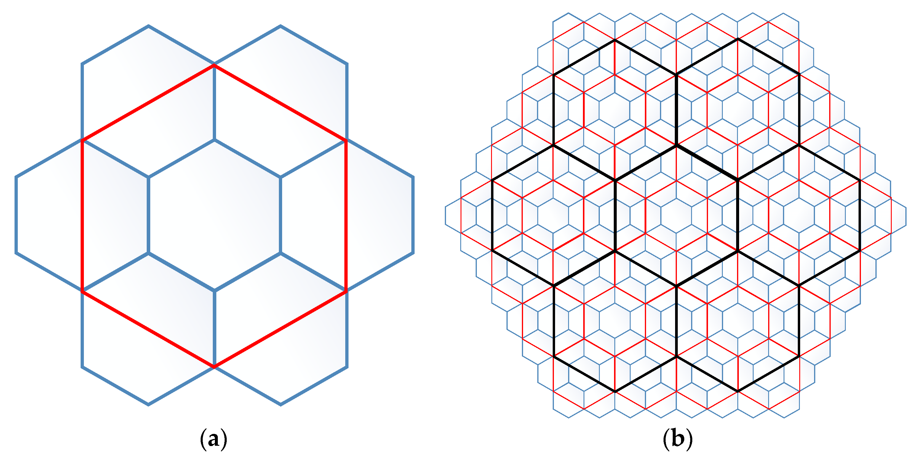
This study chose the planar aperture 4 hexagon grid system as the framework to transform the original remote sensing data, for in this system the direction of the hexagon stays consistent. The hexagonal grid planar structure is shown in Figure 1.

Firstly, the appropriate grid level needs to be selected for modeling and sampling. The expression of raster data on the grid depends on the resolution of the remote sensing image. Since the size of the grid cannot be exactly the same as the size of each pixel unit of the remote sensing image, in actual processing, the level we choose is the layer of the grid area that is slightly smaller than the area represented by each pixel of the remote sensing image. For example, each pixel of the remote sensing image represents 4 square meters, the size of a single grid on the 22nd layer is about 3.86 square meters, and the size of a single grid on the 21st layer is about 15.26 square meters. According to this standard, Landsat 8 images with a resolution of 30 m can be stored on the 18th layer, and images with a resolution of about 1 km can be stored on the 13th layer. On the selected level, the correspondence between each grid and the raster data in the remote sensing image should be determined. Since the area of each grid of the grid that we selected to store a certain remote sensing image is smaller than a single pixel of the remote sensing image, each grid can store the pixel value of the grid with the largest area so as to minimize the loss of the original remote sensing image data. The basic process is as follows.

The first step to determine the level of the hexagonal grid corresponding to the remote sensing image pixel according to the spatial resolution of the remote sensing image, and the corresponding discrete grid level should meet the requirement of $n_1\le n\le n_2$. Then, based on the correspondence between geographic coordinates and hexagonal grid coding, a conversion model between remote sensing data and hexagonal grid data is established.

Hexagonal grids of different levels have corresponding areas of hexagonal elements. The best division area when dividing the grid is:

$$s=\frac{\mathrm{SR}\times \mathrm{m}}{\mathrm{MR}}$$

(1)

where SR is the area of remote sensing image, MR is the size of remote sensing image, and m is preset size of the remote sensing image after subdivision. The grid levels corresponding to remote sensing images of different resolutions calculated by formula (1) are shown in

Table 1. Grid levels corresponding to commonly used high-, medium-, and low-resolution remote sensing images.

Remote Sensing Data	Remote Sensing Data	Spatial Resolution	Number of Bands	Adjacent Grid Level	Corresponding Grid Level
Low-spatial-resolution remote sensing data	NOAA/AVHRR	1.1 km	5	12.13	13
	Modis	250–1000 m	36	13.14	13
	Spot Vegetation	1000 m	4	12.13	13
Medium-spatial-resolution remote sensing data	Landsat 8	30 m	11	18.19	18
	Spot 5	10 m	6 Multispectral (4), Panchromatic (1), Shortwave infrared (1)	19.20	19
	Terra/aster	15 m	14	19.20	19
High-spatial-resolution remote sensing data	Quick Bird	1 m	5	22.21	22
	Eros-b Satellite	0.41 m	1	22,23	22
	Eros-a Satellite	1.9 m	1	22.21	22

.

When converting a rectangular grid into a hexagonal grid, the spatial resolution of the hexagonal grid (the size of the cells) can be determined according to the spatial resolution of the rectangular grid. Generally, the resolution of a rectangular grid corresponds to the hexagonal grid between two adjacent layers, rather than the area of a certain layer of hexagonal units. In this way, it is necessary to determine which layer should be converted to and the six sides of the corresponding layer. The absolute value of the difference between the area of the rectangular element and the area of the rectangular element should be the smallest.

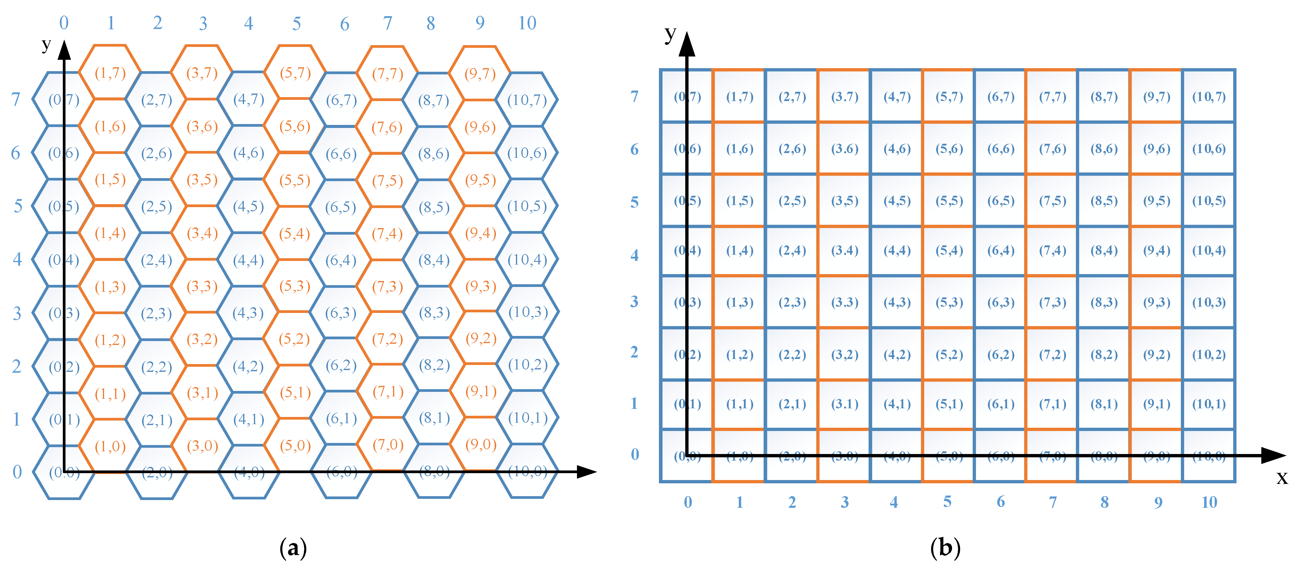
In order to determine the correspondence between grid coordinates and geographic coordinates, we used the concept of “point to raster” to establish a planar hexagonal grid based on an orthogonal coordinate system. As shown in Figure 2, the number of rows and columns (i, j) where the grid is located is coded, and (0, 0) is the origin of the coordinates.

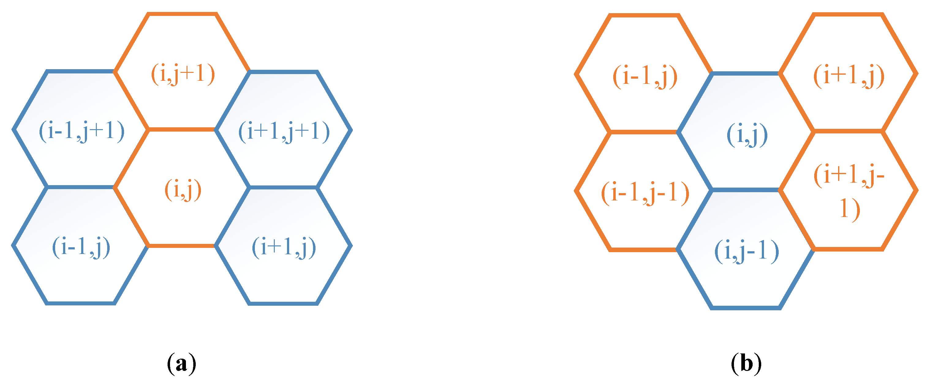
According to Figure 2, when a regular hexagon is tiled, the odd and even columns have a certain offset. If the side length of the hexagonal unit is l, then the offset between odd rows and even rows is $\frac{\sqrt{3}}{2}l$, as shown in Figure 3.

According to the idea of “rasterization” and to simplify calculations, the attributes of the hexagonal grid cells and the calculation and analysis between grids are replaced by the corresponding grid center points, thus the attribute value of each grid in the grid structure is obtained. The geographic coordinate value of the center point of the grid is a key step in the application of the hexagonal grid structure to remote sensing data. According to the above analysis, the corresponding relationship between the planar hexagonal grid and geographic coordinates can be defined as:

$$\{\begin{array}{c}Y\left(i,j\right)=\{\begin{array}{c}{y}_0+\sqrt{3}l\times j,\hspace{1em}i\%2=0\\ y_0+\sqrt{3}\left(j+\frac{1}{2}\right)l,\hspace{1em}i\%2=1\end{array}\\ X\left(i,j\right)=1.5y_0\times l\end{array}$$

(2)

where $Y\left(i,j\right)$ and $X\left(i,j\right)$ are the geographical coordinates of the grid center point with grid coordinates of (i, j), and $l$ is the side length of the hexagonal grid cell. Then, on a two-dimensional plane, the specific study area is filled with hexagonal grids, and the pixels of the remote sensing image are resampled with the following resampling methods to determine the attribute value of the hexagonal grid unit.

The nearest-neighbor interpolation takes the gray value of the nearest-neighbor among the four neighboring pixels around the point to be sampled as the gray value of the point. It only uses the gray value of the pixel that has the greatest impact on the sampling point (that is, the nearest) as the value of the point, which is simple to calculate. It does not take the influence (correlation) of other adjacent pixels into consideration, thus there might be obvious discontinuities, and the image distortion cannot be ignored.

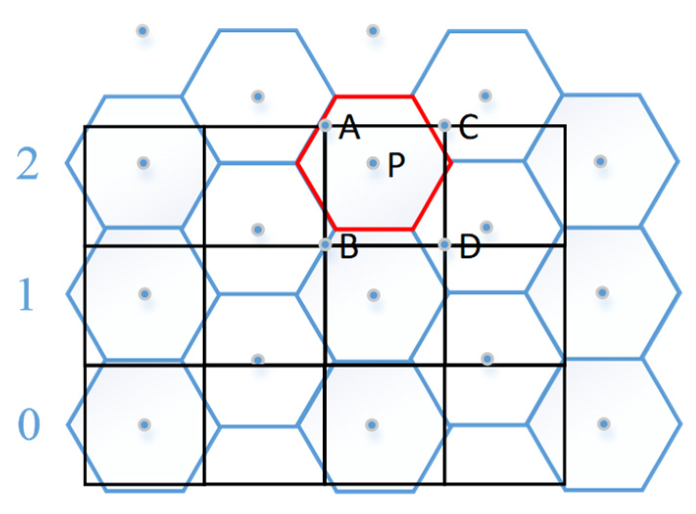
As an improvement to the nearest-neighbor method, bilinear interpolation uses the gray values of the surrounding 4 neighboring points to perform linear interpolation in two directions to obtain the gray value of the point to be sampled; that is, the corresponding weight is determined according to the distance between the point to be sampled and the adjacent point to calculate the gray value of the point to be sampled, as shown in Figure 4.

According to Figure 4, the pixel value of P is determined by A, B, C, and D, and the attribute value of the red-edged hexagon unit is determined by the value of P. Compared with the nearest-neighbor interpolation, the bilinear interpolation method takes the influence of the four direct neighbors around the sampling point on the sampling point into consideration, which basically overcomes the shortcomings of the former gray scale discontinuity, but the amount of calculation is increased.

The cubic convolution method not only considers the influence of the gray value of the four direct neighboring points but also the influence of the gray value change rate between the neighboring points. It uses 16 points to be sampled. The gray values of pixels in the larger surrounding neighborhood are interpolated three times.

The sampled grid data need to be stored as the coordinates of the center of the hexagon, the direction, size, and attribute values of the hexagon. When this information is read, an image based on the hexagonal grid can be reproduced based on the information.

2.2. Accuracy Evaluation of Hexagonal Grid Data

Since the original remote sensing images are also obtained by sampling and quantization, the image itself has errors, and after the image is interpolated, the error is transferred to the new sampled points through interpolation, the error transfer needs to be quantified, and the hexagonal-based remote sensing image needs to be compared with the original image [33,34] by calculating the loss of information and the error of geographic coordinates in the process of expression on the hexagonal grid. Therefore, it is necessary to establish an appropriate error evaluation model to evaluate the error of the converted data.

The relevant elements involved in the comprehensive evaluation of a certain thing constitute the evaluation element set. A series of indicators used to evaluate the thing constitute the evaluation index set, of which the weights are not the same. The evaluation index set is a mapping of the evaluation elements set [32,35], where there are multiple mapping index sets for an evaluation element set. There are currently two typical standards for the principle of establishing an index system. The first one is comprehensive and nonoverlapping (or redundant), of which indicators are easy to obtain; the second is scientific, rational, and applicable [16,36]. According to the three criteria for evaluating the accuracy of spatial data conversion (maintaining the conservation of composition information, maintaining the conservation of area information, and maintaining the conservation of regional spatial pattern and morphological information), this research proposes evaluation indicators from three perspectives: basic evaluation indicators, evaluation indicators based on image features, and geometric evaluation index [37,38,39].

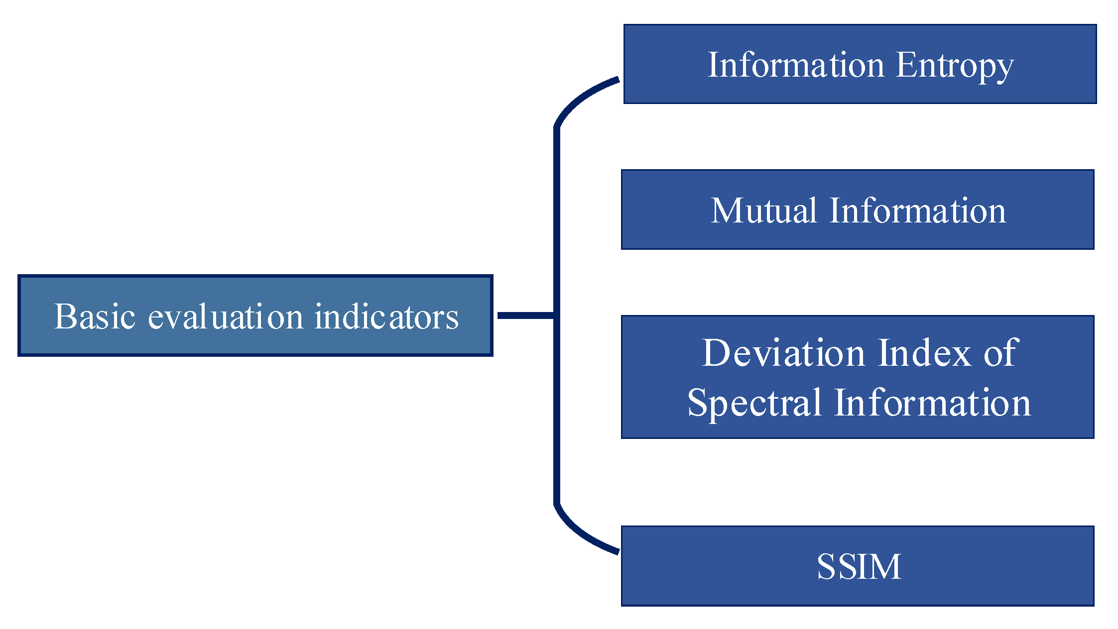
2.2.1. Basic Evaluation Indicators

The basic evaluation index is a set of evaluation indices established based on statistical information such as the mean, variance, and covariance between the original remote sensing image and the grid remote sensing image. These indicators are mainly used to evaluate the image composition information before and after conversion, with clear connotation, a simple model, and convenient evaluation. However, the basic evaluation indicators only focus on the information amount and composition type of the image, and they cannot reflect the image structure and image feature information.

From the perspective of remote sensing image analysis and application, this article selects information entropy, mutual information, combination entropy, and the structural similarity index (SSIM) to evaluate the quality of the converted remote sensing image as specified in Figure 5.

(1)

Information entropy

Information entropy reflects the information richness of the image, and calculating the information entropy of the image before and after conversion can reflect the loss of information during the conversion process [40]. If the amount of change in information entropy before and after the data conversion is small, it means there is not much information loss during the process. The calculation formula is as follows:

$$m_k=\frac{1}{N_k\times M_k}{\displaystyle \sum }_{j=1}^{N_k}{\displaystyle \sum }_{i=1}^{M_k}p\left[C_k\left(i,j\right)\right]lo{g}_2\left|C_k\left(i,j\right)\right|$$

(3)

where $P\left(I\right)$ is the probability that a certain pixel value I appears in the image, and N is the pixel value range (usually 0–255). In order to quantify the information entropy of the images before and after the conversion, this paper performs a ratio operation on the information entropy of the images before and after the conversion, and the closer the information entropy of the two images is to 1, the less information is lost during the conversion process.

(2)

Mutual information

Mutual information is an important concept in information theory. It can be used as a measurement of the correlation between two variables or a measurement of the amount of information contained in another variable. Suppose there are two random variables$P_X\left(x\right)$ and $P_Y\left(y\right)$, their marginal probability distributions are A and B, and their joint probability density is $P_{XY}\left(x,y\right)$. According to the related concepts of information theory, the mutual information between these two variables is:

$$M_{XY}\left(x,y\right)={\displaystyle \sum }_{x,y}{P}_{xy}\left(x,y\right)$$

(4)

An image can be regarded as a two-dimensional random variable. The above concept can be easily extended to a two-dimensional space. The two images, Images A and B, before and after conversion have the same gray level. Let the total gray level of the image be L, where $P_A\left(a\right)$ and $P_B\left(b\right)$ are the probability densities of the images before and after conversion. The probability density can be obtained by dividing the histogram of the image by the total number of pixels in the image. Therefore, the mutual information of the images before and after conversion can be defined as:

$$M_{AB}={\displaystyle \sum }_{j=0}^{L-1}{\displaystyle \sum }_{a=0}^{L-1}p{F}_A\left(f,a\right)$$

(5)

Mutual information is an objective indicator that reflects the abundance of information before and after data conversion. The larger its value, the more abundant information the hexagonal grid data can obtain from remote sensing data, and it can accurately evaluate the accuracy of the conversion.

(3)

Deviation Index of Spectral Information

The deviation index of the spectral information can reflect how the spectral information of the image after data transformation and resampling and the original image match with each other. The main calculation method is to transversely calculate the ratio of the absolute value of all the pixel values of the image and the pixel value of the original image to the pixel value of the original image. The formula is:

$$D=\frac{1}{MN}{\displaystyle \sum }_{i=1}^M{\displaystyle \sum }_{j=1}^N\frac{\left|B\left(i,j\right)-A\left(i,j\right)\right|}{A\left(i,j\right)}$$

(6)

where $A\left(i,j\right)$ is the original remote sensing image at coordinates $\left(i,j\right)$ before conversion, and $B\left(i,j\right)$ is the pixel value at coordinates $\left(i,j\right)$ of the converted hexagonal remote sensing image. The smaller the deviation index D, the better the spectral information of the original image, Image A, is preserved.

(4)

Structural similarity index (SSIM)

Structural similarity index establishes an image distortion evaluation model from the three factors of brightness, contrast, and structure in terms of identifying things with human eyes. In this evaluation model, the mean is the estimated value of brightness, the standard deviation is the estimated value of image contrast, and the covariance can be used as a measure of the structural similarity of the image using the mean. This index can be used to compare the structural information of the image, thereby analyzing the distortion of the image and objectively evaluating the image before and after conversion.

$$SSIM\left(A,B\right)=\frac{\left(2u_A{u}_B+c_1\right)\left(2{\sigma }_{AB}+c_2\right)}{\left(u_A^2+u_B^2+c_1\right)\left({\sigma }_A^2+{\sigma }_B^2+c_2\right)}$$

(7)

where $u_A,u_B$ are the average of A, B,${\sigma }_{AB}$ is the covariance of Images A and B,${\sigma }_A^2$ and ${\sigma }_B^2$ are the variance of Images A and B, and B; $c_1={(k_{1}L)}^2,c_2={(k_{2}L)}^2$ are constants to maintain stability, in which $k_1=0.001 \mathrm{and} k_2=0.03.$

2.2.2. Evaluation Index Based on Image Construction

The edge structure similarity (ESSIM) can reflect the edge information of the hexagonal grid image obtained from the source image during the conversion process.

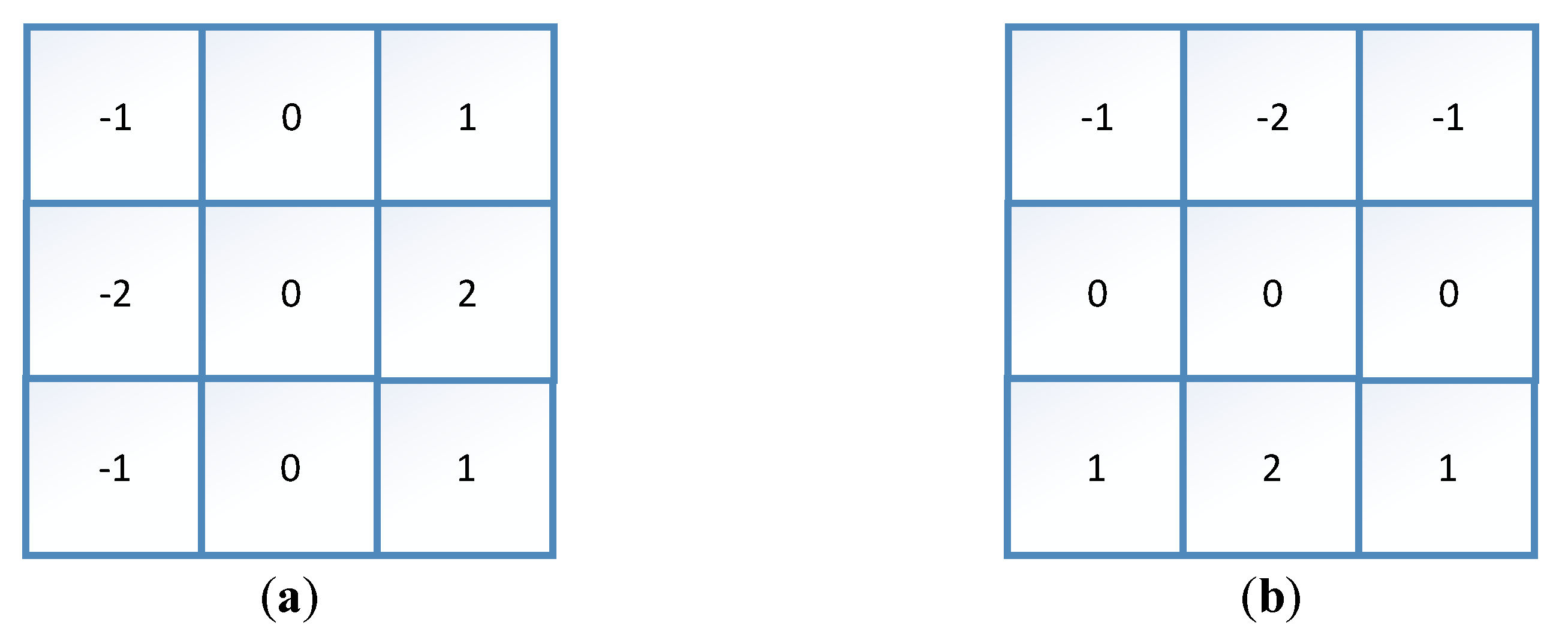
For the original remote sensing image composed of quadrilateral pixels, the Sobel operator is used to calculate the gradient value in the vertical direction (y) and the horizontal direction (y), and the integrated gradient value can be calculated by Formula (15), where $S_A^x{\left(i,j\right)}^2$ and $S_A^y{\left(i,j\right)}^2$ are the horizontal and vertical amplitudes of pixels after Sobel (shown in Figure 6), respectively.

$$g_A\left(i,j\right)=\frac{\sqrt{S_A^x{\left(i,j\right)}^2+S_A^y{\left(i,j\right)}^2}}{2}$$

(8)

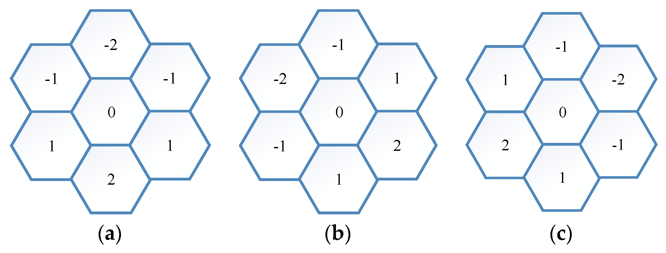
According to the geometric characteristics of the hexagonal grid, this paper proposes HSobel operators for hexagonal grid images. As shown in Figure 7, three operators are used to calculate the gradients in the three directions (x, y, z) of the hexagonal grid, and Formula (16) is used to calculate the integrated gradient.

$$g_B\left(i,j\right)=\frac{\sqrt{S_B^x{\left(i,j\right)}^2+S_B^y{\left(i,j\right)}^2+S_B^z{\left(i,j\right)}^2}}{3}$$

(9)

The relative edge strength and direction values of the hexagonal grid image, Image B, and the original image, Image A, are:

$$G^{AB}\left(i,j\right)=\{\begin{array}{c}\frac{g_B\left(i,j\right)}{g_A\left(i,j\right)}, if g_A\left(i,j\right)>g_B\left(i,j\right)\\ \frac{g_A\left(i,j\right)}{g_B\left(i,j\right)}, other wise\end{array}$$

(10)

Thus, we can get the edge retention of the converted image relative to the source image:

$$Q^{AB}\left(i,j\right)=Q_g^{AB}\left(i,j\right)Q_a^{AB}\left(i,j\right)={\mathsf{\Gamma }}_g{\mathsf{\Gamma }}_a{\left[1+e^{K_g(G^{AB}\left(i,j\right)-{\sigma }_g}\right]}^{-1}\left[1+e^{K_a(G^{AB}\left(i,j\right)-{\sigma }_{\alpha }}\right]$$

(11)

where ${\mathsf{\Gamma }}_g$,${ \mathsf{\Gamma }}_a$,${ \mathrm{k}}_g$,${ \mathrm{k}}_{\alpha }$,${ \mathsf{\sigma }}_g$,${ \mathsf{\sigma }}_{\alpha }$ are adjustable constant.

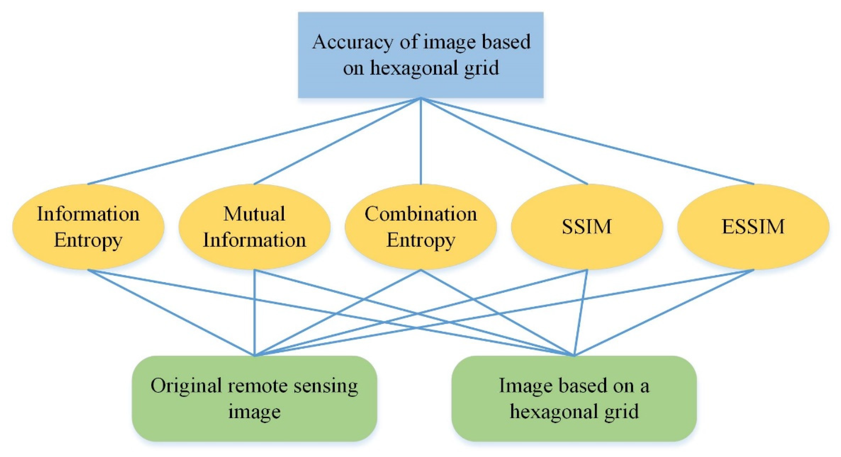
2.2.3. Normalization of Evaluation Indicators and Calculation of Weights

There may be a certain difference in the magnitude of the calculation of different indicators. In order to simplify the calculation, this article normalizes the calculation results of all indicators. The closer the index is to 1, the higher the similarity of the images before and after the conversion. In order to simplify the basic evaluation index system, we use the analytic hierarchy process to determine the weights of the five major evaluation index systems.

The first layer: the target layer. The purpose of the model is to evaluate the information retention before and after conversion of the hexagonal grid image and the similarity to the original image. Therefore, the degree of similarity is regarded as the predetermined goal of decision-making.

The second layer: the indicator layer. Through literature research, this paper selects five indicators (information entropy, mutual information, combination entropy, SSIM, and ESSIM) as indicators to quantify the preservation of image information before and after conversion, the similarity with the original image, and the structural similarity. These five indicators are intermediate evaluation standards.

The third layer: the program layer. The objects we analyze are the original remote sensing image and the sampled remote sensing image based on the hexagonal grid, thus the basic decision plan can be divided into the original remote sensing image and the hexagonal grid image.

Based on the above problem analysis, we established the following analytic hierarchy model(Figure 8):

Then, we used the analytic hierarchy process to determine the weight of the evaluation factor

(a)

Construct a judgment matrix

We used the method of paired comparison and the 1–9 scale to construct the decision Matrix A = ($a_{ij}$)

$$a_{ik}\times a_{kj}=a_{ij}$$

(12)

where $a_{ij}$is set by standards of 1~9.

According to the Delphi method, the following judgment matrix is constructed:

$$A=\left(\begin{array}{ccccc}1& 1/2& 4& 3& 3\\ 2& 1& 7& 5& 5\\ 1/4& 1/7& 1& 1/2& 1/2\\ 1/3& 1/5& 2& 1& 1\\ 1/3& 1/5& 3& 1& 1\end{array}\right)$$

(13)

According to the mutual influence of the five indicators, paired comparison matrices are constructed as follows:

$$B_1=\left(\begin{array}{cc}1& 3\\ 1/3& 1\end{array}\right),B_2=\left(\begin{array}{cc}1& 2\\ 1/2& 1\end{array}\right),B_3=\left(\begin{array}{cc}1& 3\\ 1/3& 1\end{array}\right),B_4=\left(\begin{array}{cc}1& 2\\ 1/2& 1\end{array}\right),B_5=\left(\begin{array}{cc}1& 3\\ 1/3& 1\end{array}\right)$$

(14)

(b)

Calculate eigenvalues

MATLAB is used to find the maximum eigenvalue of Matrix A ${\lambda }_{max}$ and the corresponding matrix vector $u={\left(u_1,u_2,\dots u_n\right)}^T$, and the following formula to normalize u.

$$x_i=\frac{u_i}{{{\displaystyle \sum }}_{i=0}^n{u}_j}$$

(15)

(c)

Consistency inspection

Calculate the consistency index CI:

$$CI=\frac{{\lambda }_{max}-n}{n-1}$$

(16)

Calculate the consistency ratio CR:

$$CR=\frac{CI}{RI}$$

(17)

According to the calculation, we get CR = 0.0145 < 0.1, which means that the matrix has already passed the consistency check.

In terms of paired comparison matrices $B_1,B_2,B_3,B_4,B_5$, we can find the weight vector of the hierarchical total sorting and perform the consistency test. Through calculation, it can be known that $B_1,B_2,B_3,B_4,B_5$ passed the consistency test.

Then, we calculated the total ranking weight and consistency test. According to the calculation, the weights of B on the overall goal are as shown in

Table 2. Consistency index of the five evaluation indexes.

k	Information Entropy	Mutual Information	Combination Entropy	SSIM	ESSIM
CR	0.0048	0.0013	0.0025	0.0079	0.0014

.

CR < 0.1. Thus, total ranking passes the consistency test. And the weight of the objective options are shown in

Table 3. Weight of the objective options.

Objective	Original Remote Sensing Image	Hexagonal Pixel Image
CR	0.5179	0.4821

.

Thus, the weight of each index can be determined: information entropy: 0.21, mutual information: 0.18, combination entropy: 0.24, SSIM: 0.24 and ESSIM: 0.17.

2.2.4. Geometric Evaluation Index

In addition, this study also calculated the change in the DN value of the pixel unit and in line length $l_c$ before and after sampling.

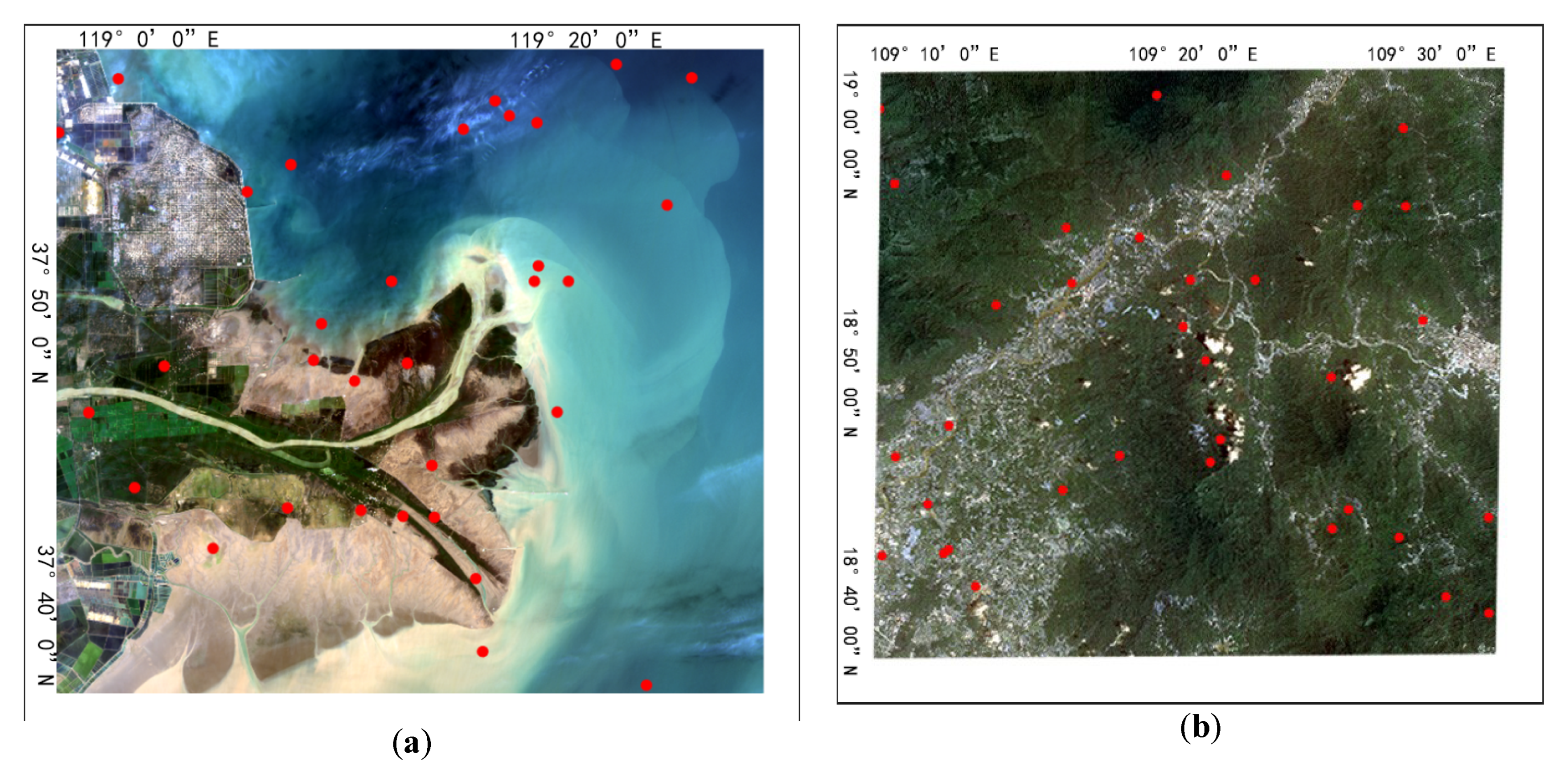
In order to evaluate the credibility of the generated hexagonal grid image, this paper uses the checkpoint method. We randomly select 30 feature points in a scene image as the checkpoints and use the RMSE of the pixel value to perform the accuracy evaluation of the remote sensing image based on the hexagonal grid. The formula is:

$$RMSE=\sqrt{\frac{{{\displaystyle \sum }}_i^n{\left(H_i-S_i\right)}^2}{n}}$$

(18)

where $H_i\left(i=1,2,\dots ,n\right)$ is the pixel value of the checkpoint on the original image, $S_i$ is the pixel value of the remote sensing image based on the hexagonal grid, and RMSE is the root mean square error of the pixel value.

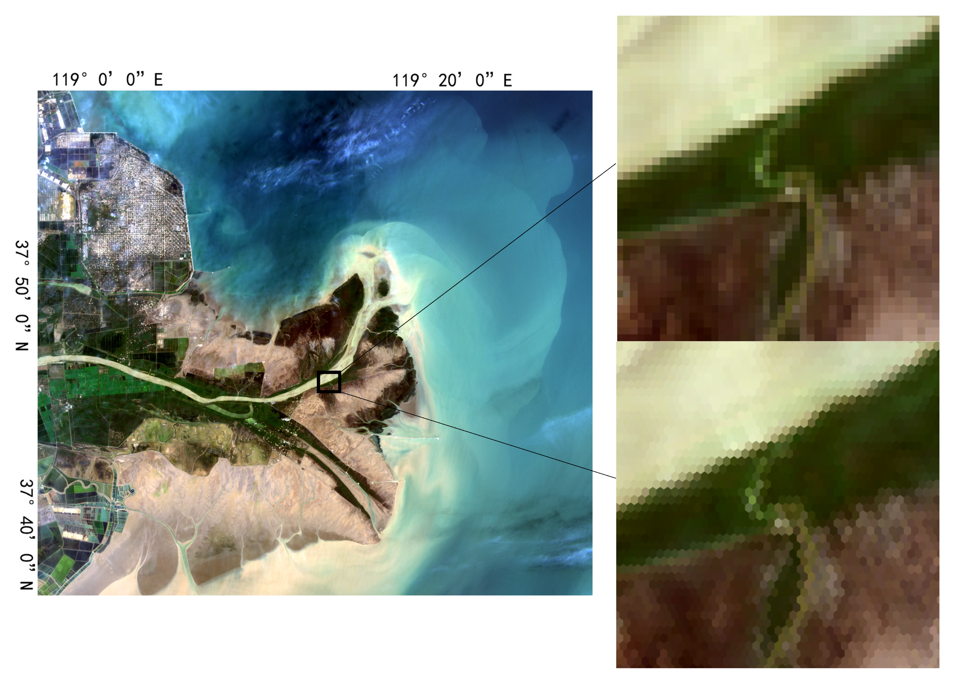
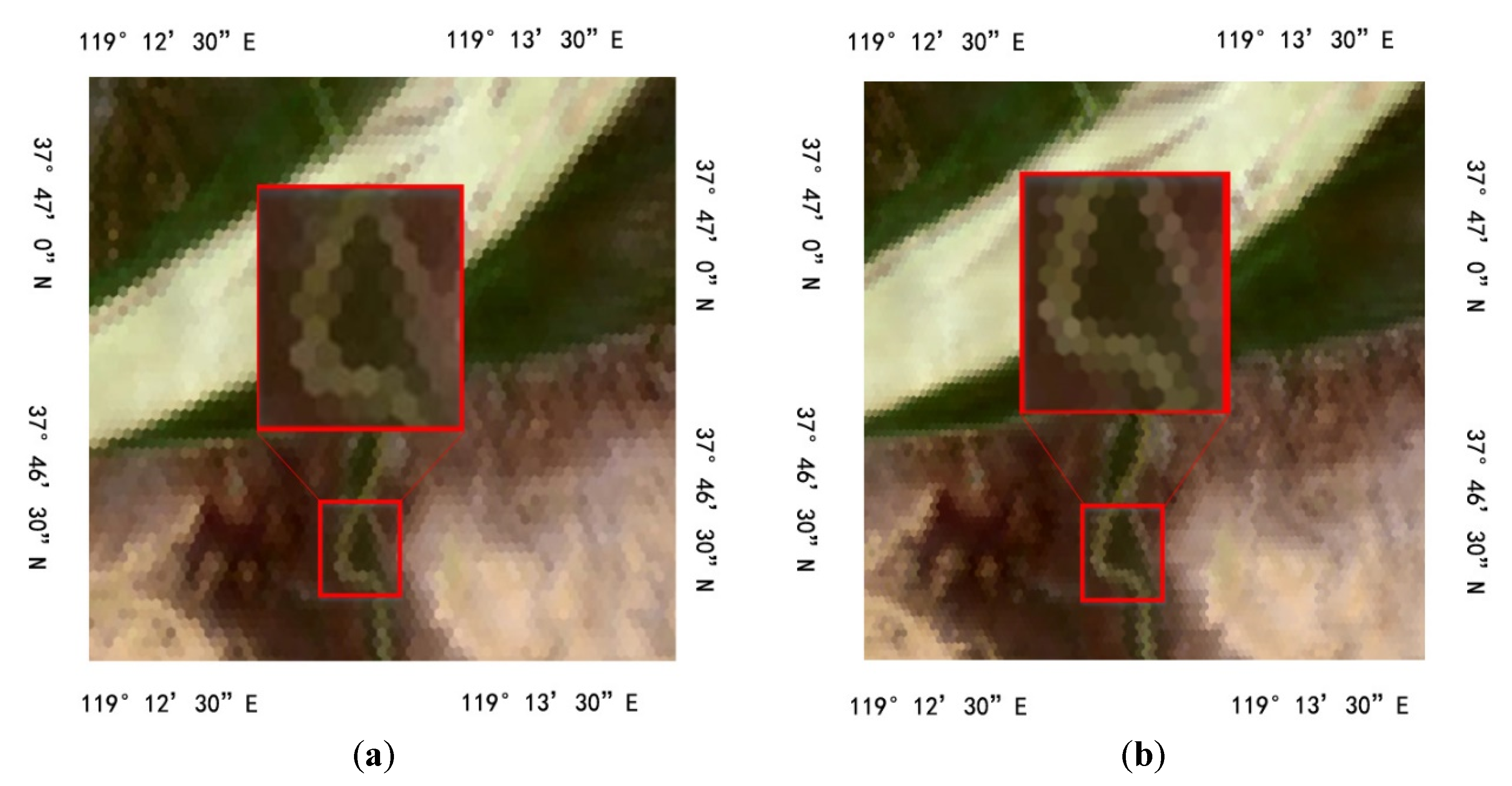
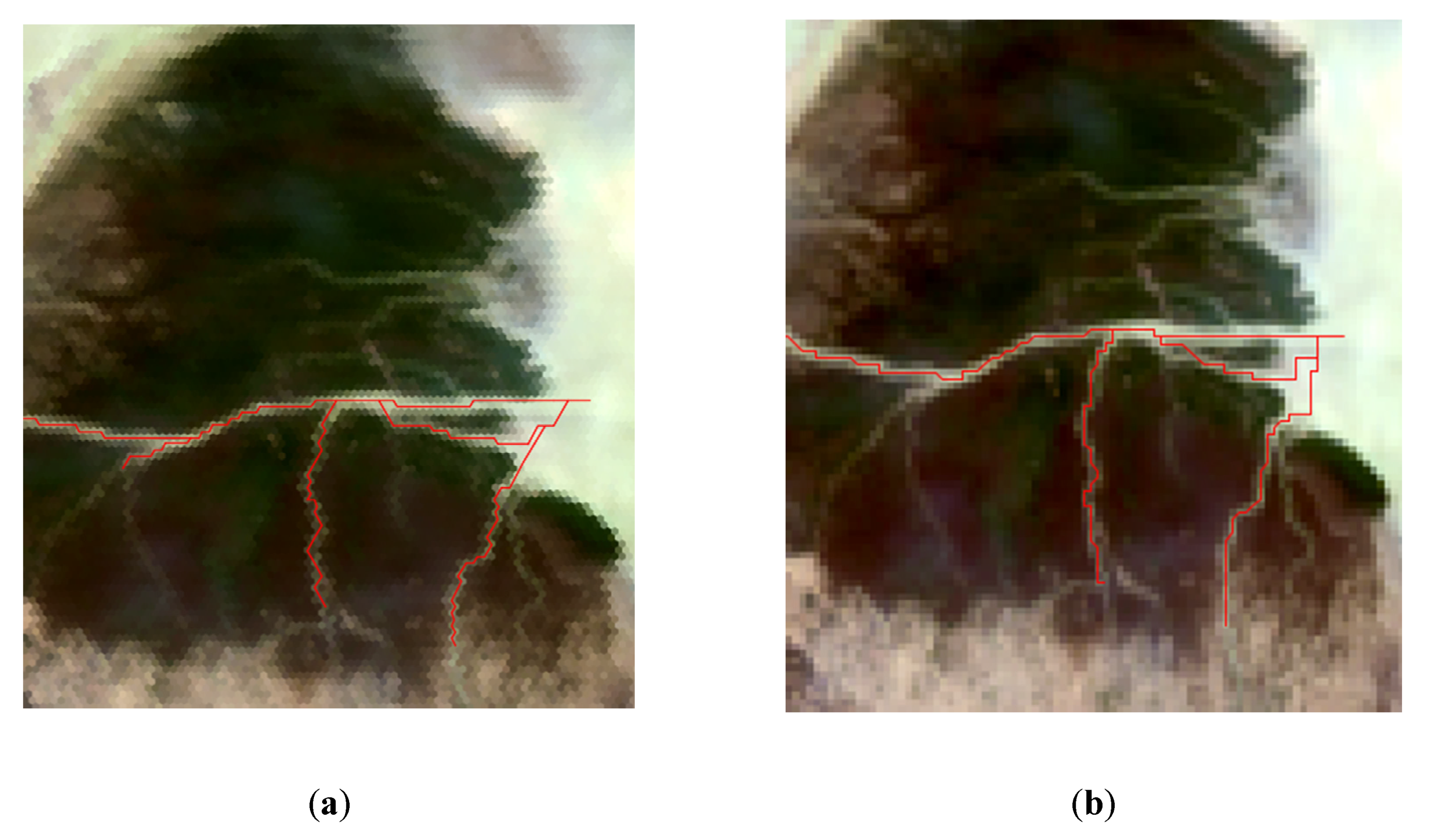
In order to evaluate the retention of the geometric features of the image during the image conversion process, this paper performs a refinement operation on the local area of the Landsat 8 images before and after the conversion, and compared the differences between the two.

When refining the same target, the hexagonal refinement algorithm only needs six templates, and each template includes 7 units, while the square refinement requires 8 templates, and each template requires 9 units as shown in

Table 4. Comparison of the refinement zero conditions of rectangular pixels and hexagonal pixels.

	Zero condition		Zero condition
	1.$2\le NZ\left(P1\right)\le 6$;		1.$2\le NZ\left(H1\right)\le 6;$
	2.$Z0 \left(P1\right)=1;$		2.$Z0 \left(H1\right)=1;$
	3.$P2\times P4\times P8=0;$		3.$H2\times H4\times H6=0;$
	4.$P2\times P4\times P6\times P9=0$		4.$H3\times H5\times H7=0$

.

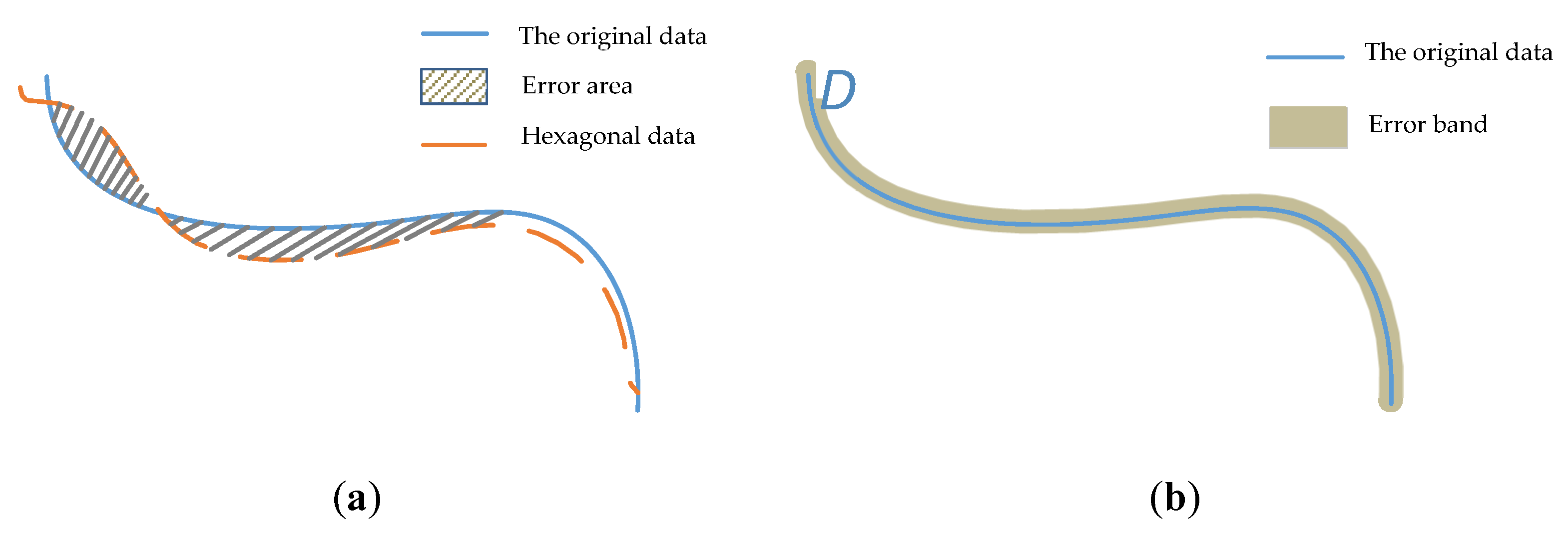
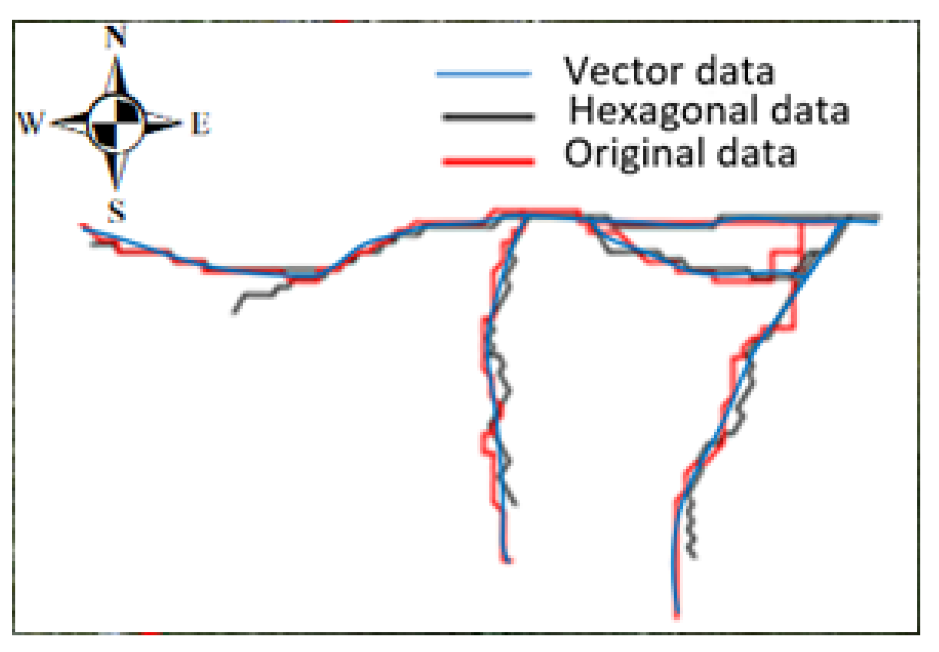
In order to quantitatively analyze the results of the refinement of linear features, this paper uses the error band to indicate the degree of deviation between the original image refinement results and the hexagonal grid image refinement results [29].

$$D=\frac{\Delta s}{L}$$

(19)

where $\Delta s$ is the error area between the linear features extracted by the two image formats, and this parameter is the number of grid cells between the two linear features multiplied by the cell area. As shown in Figure 9, L is the average length of linear elements extracted by the two image formats, which is determined by the number of grid cells through which the linear elements pass. D is the average error width under this length.

This parameter can quantify the degree of agreement between the linear elements extracted from the original image and the hexagonal grid image.

3. Results

3.1. Remote Sensing Data Modeling Based on Hexagonal Grids

3.1.1. Introduction of Data and Study Area

Landsat 8 is a land satellite launched by NASA on 11 February 2013. The satellite carries two main payloads: OLI and TIRS. The spatial resolution is 30 m (15 m in the panchromatic band). This article uses the Landsat 8 image of the Yellow River mouth area downloaded from USGS

The GF-1 satellite is a group of application satellites developed by the Aerospace Dongfanghong Satellite Co., Ltd. of the Space Technology Research Institute affiliated to the China Aerospace Science and Technology Corporation. It was successfully launched by the Long March 2D carrier rocket at the Jiuquan Satellite Launch Center on 26 April 2013. emission. The GF-1 satellite is equipped with two 2 m resolution panchromatic/8 m resolution multispectral cameras and four 16 m resolution multispectral cameras. The satellite project broke through the optical remote sensing technology. It combined high spatial resolution, multispectral and high time resolution, multiload image splicing and fusion technology, high-precision and high-stability attitude control technology, a five- to eight-year lifespan, high-reliability satellite technology, and high-key technologies such as resolution data processing and application. The data used in this article comprise a high-resolution image of Hainan with a resolution of 2 m.

3.1.2. Result Comparison

The nearest-neighbor interpolation, bilinear interpolation, and cubic convolution interpolation methods are used to convert remote sensing images of different resolutions (high-, medium-, and low-resolution, respectively, using GF-1, Landsat 8 images as examples) to data based on hexagonal grids.

The conversion of remote sensing data to hexagonal grid data includes two steps: the first step is the construction of the regional hexagonal grid; the second step is the remote sensing data sampling based on the hexagonal grid. First, it is necessary to determine the four-corner coordinates of a scene of remote sensing data and determine the scope of grid construction according to the four-corner coordinates. Secondly, the unit size of the hexagonal grid is determined according to the spatial resolution of the remote sensing image. For example, the spatial resolution of Landsat 8 is 30 m; then, according to Formula (1) and Table 1, it can be determined that the grid level corresponding to Landsat 8 is 18 layers, and the area of the hexagonal unit of the grid on the 18th layer is 989.657 square meters. After determining the scope of grid construction and the grid level, we can fill in the hexagonal grid of the corresponding level within the four-corner coordinates of the remote sensing image, as shown in Figure 10.

Using different resampling methods to convert remote sensing images in the same area into hexagonal grid images has different effects. Figure 11 shows the interpolation results of Landsat 8 images in the same area (Yellow River Estuary) using different interpolation methods. It can be clearly seen that, compared with nearest-neighbor interpolation, bilinear interpolation and bicubic interpolation perform pixel-value operations, and the image is smoother. The pixel value of the nearest interpolation has not been calculated, thus the original characteristics of the remote sensing image can be better maintained, and the result of linear interpolation is smoother; for example, the boundary of the river channel does not appear jagged. The result of cubic interpolation can reflect more information and image features, but the calculation of a single pixel involves 16 adjacent pixels, which requires more work.

Figure 11 shows the results of the conversion of Landsat 8 (Yellow River Estuary Region) images using bilinear interpolation. In order to compare the calculation efficiency of different interpolation methods, the calculation time of the same scene data is recorded and compared in

Table 5. Calculation efficiency of different interpolation methods.

Data	Interpolation Method	Calculation Time
Landsat 8 (7761,7881)	Nearest-neighbor interpolation	134 s
	Bilinear interpolation	257 s
	Bicubic interpolation	452 s
GF-1 (1137,11,25)	Nearest-neighbor interpolation	16 s
	Bilinear interpolation	68 s
	Bicubic interpolation	104 s

.

The side length ratio of the hexagons between adjacent grid levels is 1:2. As shown in Figure 12, the grid unit side length ratio of the 19th grid level and the 18th grid level is 1:2, and the image of the 19th grid level can show more information and image details.

3.2. Accuracy Evaluation of Different Interpolation Methods

3.2.1. Basic Evaluation Indicators

This study calculated the basic evaluation indicators of Landsat 8 and GF-1 remote sensing images before and after conversion, as shown in

Table 6. Evaluation results based on basic evaluation indexes and image structure evaluation indexes.

Image	Interpolation Method	Information Entropy	Mutual Information	Deviation Index	SSIM	ESSIM	Comprehensive Index
Landsat 8	Nearest-neighbor interpolation	0.989	1.028	1.022	0.987	0.965	0.9968
	Bilinear interpolation	0.978	1.042	1.012	0.981	0.964	0.9972
	Bicubic interpolation	0.984	1.047	1.019	1.011	0.958	1.0040
GF-1	Nearest-neighbor interpolation	0.973	1.021	1.021	0.978	0.969	0.9937
	Bilinear interpolation	0.972	1.043	1.017	1.008	0.964	1.0016
	Bicubic interpolation	0.977	1.028	1.015	0.974	0.960	0.9958

.

The result of bilinear interpolation is closest to one. This shows that compared with the original image, the hexagonal grid image obtained by bilinear interpolation retains the most information and structural features. The main reason is that in the process of using nearest-neighbor interpolation, although the bilinear interpolation is smoothed, it uses the gray values of multiple surrounding pixels, thus the original information of the image can be better preserved. Although the cubic convolution interpolation also uses multiple surrounding pixels to calculate the interpolation result, the calculation efficiency of the cubic convolution interpolation is too low, and it is not suitable for large-scale calculations.

3.2.2. Evaluation Index Based on Image Feature

(1)

Accuracy evaluation for points

The following(Figure 13) are the results of random points selection of Landsat 8 and GF-1 remote sensing images:

Figure 13 is a schematic diagram of randomly selected checkpoints for a scene image to calculate. It can be seen that selecting thirty checkpoints for a scene image can basically cover different types of features, thus the degree of retention of the point feature of the hexagonal grid image can be calculated for the original image.

The resolution of the GF-1 image and the Landsat 8 image is not the same. The spatial resolution of the Landsat 8 OLI land imager is 30 m, and the spatial resolution of the GF-1 PMS image is 16 m. As shown in

Table 7. RMSE of hexagon-gridded images from different data resources.

Image	Interpolation Method	RMSE of the Grid Pixel Value
Landsat 8	Nearest-neighbor interpolation	7.48
	Bilinear interpolation	6.54
	Bicubic interpolation	8.06
GF-1	Nearest-neighbor interpolation	11.3
	Bilinear interpolation	10.5
	Bicubic interpolation	12.4

, we calculated the RMSE of the pixel value of the checkpoint on images obtained by different sampling methods. Among the three interpolation methods, the RMSE value of the bilinear interpolation is the smallest. The main reason is that although the process of establishing a hexagonal grid is regular, a scene is shifted compared with the coordinates of the quadrilateral pixels. Therefore, only using the nearest-neighbor interpolation operation is likely to cause a collective misalignment of pixels. The bilinear interpolation can guarantee higher interpolation accuracy.

(2)

Accuracy evaluation for the line

As shown in Figure 14, the sensitivity of the hexagonal grid image to angle changes is better than that of the original image. It is better than the quadrilateral image in terms of maintaining traits and can maintain the curved characteristics of linear features well. Hexagonal elements have a consistent direction and better angular resolution than quadrilateral elements. The quadrilateral has two directions, and the distance between these two directions is 1 and $\sqrt{2}$.

In order to compare the effects of the hexagonal grid with the original image’s retention of the curve, this paper uses the vector diagram of the Yellow River mouth area to calculate the error band between the two extracted linear features and the true value, as shown in Figure 15 and

Table 8. Error band of different data resources.

	Vector Data	Hexagonal Data	Original Data
Vector data	0	19.6	20.7
Hexagonal data	19.6	0	22.3
Original data	20.7	22.3	0

.

According to Equation (19), it can be calculated that the width of the error band between the hexagonal image and the original image is 22.3 m. The error band width between the hexagonal image and the vector image is smaller than that between the original image and the vector image, which means that because of the consistency, the hexagon can maintain the degree of curvature and directionality of the curve better.

3.2.3. Accuracy Evaluation for the Evaluation Index System

The evaluation indicators proposed in this paper include statistical indicators for the entire image and indicators based on geographic applications. In order to verify the operational efficiency of the evaluation index system, we recorded the calculation time of each index, as shown in

Table 9. Accuracy evaluation for the evaluation index system.

	Calculation Time (/s)
Information Entropy	0.00
Mutual Information	0.00
Deviation Index	0.00
SSIM	0.04
ESSIM	0.21
Accuracy evaluation for points	1.21
Accuracy evaluation for the line	2.45

.

As shown in Table 9, the calculation time of each evaluation index for the same scene image (Landsat 8 Yellow River Estuary area) is within 3 s, thus the calculation efficiency of this evaluation index system meets the general requirements.

4. Discussion

The storage of raster remote sensing data on the grid plays a vital role in subsequent applications and the integration of multisource heterogeneous data. The hexagonal grid and the original remote sensing data are two different forms of data management and data storage, and there are big differences in pixel units. This study proved that the remote sensing data based on the hexagonal grid has practical applications. Availability requires quantitative indicators to prove the similarity between the hexagonal grid data and the original data. This paper used basic evaluation indicators to prove that the amount of information in the hexagonal grid data is within a controllable range compared to the original remote sensing data. There is inevitable data loss and smoothing, but the amount of lost data is within an acceptable range. This study compared different resampling methods, including nearest-neighbor interpolation, linear interpolation, and cubic interpolation. The weights calculated in this study are not the only indicator weights. When used in different application scenarios, other appropriate judgment matrices can be selected according to the focus of remote sensing applications so as to determine the weights of different indicators accordingly.

The calculation results of the quantization index show that the image obtained by the bilinear interpolation is the closest to the original image and retains more information. In addition, based on the differences between hexagons and quadrilaterals, this paper proposed a new algorithm for thinning hexagonal grid images and further compares the linear features obtained by the thinning algorithm. It also shows that the hexagonal grid image is available in remote sensing geometry applications; for example, large area yield estimation, land use classification, river extraction, etc., based on a hexagonal grid image. In addition, according to the feature that the level of the hexagonal grid can be infinitely divided, the grid can be used to store unstructured emerging spatial big data, including point, line, human activity, luminous, etc., data. 2004

5. Conclusions

This research brought up and implemented the conversion method from the original remote sensing image to the hexagonal discrete grid image. It was dedicated to finding a suitable way to express the remote sensing data on the discrete grid and establishing a suitable accuracy evaluation system to evaluate the accuracy of the modeling aims of the remote sensing data based on the hexagonal grid. This paper proposes a targeted evaluation method for hexagonal grid images from different levels. The evaluation scope includes changes in image information, edge changes, spectral changes, and changes in feature extraction based on geographic applications. These evaluation index systems can basically comprehensively evaluate remote sensing images based on hexagonal grids. This proved their availability and provides support for the further use of remote sensing data based on hexagonal grids. The converted hexagonal data can maintain the basic and geometric characteristics of the original data. However, due to the geometrical characteristics of the hexagon grid compared to the quadrilateral grid, the direction and angle of the hexagonal data are more sensitive to line elements, which means the hexagonal grid can keep the direction better. Among the three resampling methods, the image obtained by bilinear interpolation has the highest similarity to the original image. Bilinear interpolation can ensure good operation efficiency, and it can also ensure relatively high interpolation accuracy.

References

1. Guo, H. Big Earth data: A new frontier in Earth and information sciences. Big Earth Data 2017, 1, 4–20. [Google Scholar] [CrossRef] [Green Version]
2. Yao, X.; Li, G.; Xia, J.; Jin, B.; Zhu, D. Enabling the Big Earth Observation Data via Cloud Computing and DGGS: Opportunities and Challenges. Remote Sens. 2019, 12, 62. [Google Scholar] [CrossRef] [Green Version]
3. Nan, L.; Cheng, C.; Ma, H.; Yang, Y. Global Discrete Grid Systems Analysis and Comparison. In Proceedings of the Geoscience & Remote Sensing Symposium, Munich, Germany, 22–27 July 2012. [Google Scholar]
4. Sahr, K.; White, D.; Kimerling, A.J. Discrete Global Grid System. Cartogr. Geogr. Inf. Sci. 2003, 30, 121–134. [Google Scholar] [CrossRef] [Green Version]
5. Sahr, K.; White, D.; Kimerling, A.J. Geodesic Discrete Global Grid Systems. Am. Cartogr. 2003, 30, 121–134. [Google Scholar] [CrossRef] [Green Version]
6. Yao, X.; Li, G. Big spatial vector data management: A review. Big Earth Data 2018, 2, 108–129. [Google Scholar] [CrossRef]
7. Sirdeshmukh, N. Utilizing a Discrete Global Grid System For Handling Point Clouds With Varying Locations, Times, and Levels of Detail. Cartogr. Int. J. Geogr. Inf. Geovisualization 2018, 541, 4–15. [Google Scholar] [CrossRef] [Green Version]
8. Goodchild, M.F.; Kimerling, A.J.E. Discrete Global Grids: A Web Book; eScholarship; National Center for Geographic Information and Analysis (UCSB): Santa Barbara, CA, USA, 2002. [Google Scholar]
9. Asharindavida, F. Study on Hexagonal Grid in Image Processing. Int. Proc. Comput. Sci. Inf. Tech 2012, 7–8. [Google Scholar]
10. Kazi Mostafa, I.H. An edge detection method for hexagonal images. Int. J. Image Process. 2016, 10, 12. [Google Scholar]
11. Jasiewicz, J.; Stepinski, T.; Niesterowicz, J. Multi-scale segmentation algorithm for pattern-based partitioning of large categorical rasters. Comput. Geosci. 2018, 118, 122–130. [Google Scholar] [CrossRef] [Green Version]
12. Wang, L.; Ai, T.; Shen, Y.; Li, J. The isotropic organization of DEM structure and extraction of valley lines using hexagonal grid. Trans. Gis. 2020, 24, 483–507. [Google Scholar] [CrossRef]
13. Zhou, J.; Ben, J.; Wang, R.; Zheng, M.; Yao, X.; Du, L. A novel method of determining the optimal polyhedral orientation for discrete global grid systems applicable to regional-scale areas of interest. Int. J. Digit. Earth 2020, 13, 1553–1569. [Google Scholar] [CrossRef]
14. Her, I. Geometric transformations on the hexagonal grid. IEEE Trans. Image Process. 2002, 4, 1213–1222. [Google Scholar]
15. Xia, J.; Yang, C.; Li, Q. Building a spatiotemporal index for Earth Observation Big Data. Int. J. Appl. Earth Obs. Geoinf. 2018, 73, 245–252. [Google Scholar] [CrossRef]
16. Devendran, A.A.; Lakshmanan, G. A Review on Accuracy and Uncertainty of Spatial Data and Analyses with Special Reference to Urban and Hydrological Modelling. In Proceedings of the Isprs Annals of the Photogrammetry, Remote Sensing & Spatial Information Sciences, Ii-8, Isprs Technical Commission VIII Symposium, Hyderabad, India, 9–12 December 2014. [Google Scholar]
17. Freeman, L.K. WebGeochem: DGGS Geochemical Sample Analysis Search Engine. 2005. Available online: https://dggs.alaska.gov/metadata/webgeochem_app.faq.html (accessed on 22 March 2021).
18. Guo, Z. Research of Environment Monitoring System Based on Discrete Global Grids; East China Normal University Shanghai: Shanghai, China, 2008. [Google Scholar]
19. Wenshuai, Y.U.; Tong, X.; Jin, B.; Xie, J. The Accuracy Control in the Process of Vector Line Data Drawing in the Hexagon Discrete Global Grid System. J. Geo-Inf. Sci. 2015, 6, 70–76. [Google Scholar]
20. Gregory, M.J.; Kimerling, A.J.; White, D.; Sahr, K. A comparison of intercell metrics on discrete global grid systems. Comput. Environ. Urban Syst. 2008, 32, 188–203. [Google Scholar] [CrossRef]
21. White, D.; Kimerling, A.J.; Sahr, K.; Song, L. Comparing area and shape distortion on polyhedral-based recursive partitions of the sphere. Int. J. Geogr. Inf. Syst. 1998, 12, 805–827. [Google Scholar] [CrossRef]
22. Zhang, B.; Yuan, Z.Y.; Zhao, X.S.; Zhang, X.J. An Geometry Deformation Evaluation Index of the Spherical Discrete Grid Based on the Fuzzy Similarity. Geogr. Geo-Inf. Sci. 2015, 31, 20–24. [Google Scholar]
23. Sahr, K. Hexagonal discrete global grid systems for geospatial computing. Arch. Photogramm. 2011, 22, 366–376. [Google Scholar]
24. Chandio, I.A.; Matori, A.N.B.; Wanyusof, K.B.; Talpur, M.A.H.; Lawal, D.U. GIS-based analytic hierarchy process as a multicriteria decision analysis instrument: A review. Arab. J. Geosci. 2013, 6, 3059–3066. [Google Scholar] [CrossRef]
25. Li, M.; Stefanakis, E. Geo-feature modeling uncertainties in discrete global grids: A case study of downtown Calgary, Canada. Geomatica 2020, 1–21. [Google Scholar] [CrossRef]
26. Ye, S.; Liu, D.; Yao, X.; Tang, H.; Xiong, Q.; Zhuo, W.; Du, Z.; Huang, J.; Su, W.; Shen, S.; et al. RDCRMG: A raster dataset clean & reconstitution multi-grid architecture for remote sensing monitoring of vegetation dryness. Remote Sens. 2018, 10, 1376. [Google Scholar] [CrossRef] [Green Version]
27. Jin, B.; Chong, T.X.; Wang, L.; Wen, B.G. Key Technologies of Geospatial Data Management Based on Discrete Global Grid System. J. Geomat. Sci. Technol. 2010, 27, 382–386. [Google Scholar]
28. Tong, X. The Principles and Methods of Discrete Global Grid Systems for Geospatial Information Subdivision Organization. Acta Geod. Cartogr. Sin. 2011, 40, 208. [Google Scholar]
29. Ai, T.; Li, J. A DEM generalization by minor valley branch detection and grid filling. ISPRS J. Photogramm. Remote Sens. 2010, 65, 198–207. [Google Scholar] [CrossRef]
30. Wang, L.; Ai, T. The valley extraction based on the hexagonal grid-based DEM. J. Geod. Geoinf. Sci. 2019, 048, 780–790. [Google Scholar]
31. Tong, X.; Jin, B.; Qing, Z.; Zhang, Y. The hexagonal discrete global grid system appropriate for remote sensing spatial data. Proc. SPIE Int. Soc. Opt. Eng. 2009, 7146, 71460J. [Google Scholar]
32. Zhou, M.; Chen, J.; Gong, J. A pole-oriented discrete global grid system: Quaternary quadrangle mesh. Comput. Geoencesci. 2013, 61, 133–143. [Google Scholar] [CrossRef]
33. Tao, M.; Wen, Y.; Peng, G.X.; Su, L.; Wang, Z. The Study on Error Analysis of Discretization Area in Discrete Global Grid System. Procedia Environ. Sci. 2011, 10, 1122–1128. [Google Scholar] [CrossRef] [Green Version]
34. Wang, H. A Study of Evaluation Methods on Performance of the Multi-Source Remote Sensing Image Fusion. Comput. Eng. Appl. 2003, 25, 33. [Google Scholar]
35. Zhao, S.H.; Feng, X.Z.; Kang, G.D.; Elnazir, R. Multi-source remote sensing image fusion based on support vector machine. Chin. Geogr. Sci. 2002, 12, 244–248. [Google Scholar] [CrossRef]
36. Fan, S.; Zao, C.; Zou, K. A Review on the Accuracy Analysis of Spatial Scaling Data. Prog. Geogr. 2013, 31, 1574–1582. [Google Scholar]
37. Feng, X.; Qin, K.; Cui, W.; Chen, Y.; Li, X. Multiscale description and recognition of target shape in high-resolution remote sensing images. J. Remote Sens. 2014, 18, 90–104. [Google Scholar]
38. Tulloch, A.I.T.; Sutcliffe, p.; Naujokaitis-Lewis, I.; Tingley, R.; Brotons, L.; Ferraz, K.M.P.M.B.; Possingham, H.; Guisan, A.; Rhodes, J.R. Conservation planners tend to ignore improved accuracy of modelled species distributions to focus on multiple threats and ecological processes. Biol. Conserv. 2016, 199, 157–171. [Google Scholar]
39. Xu, H.Y.; Liu, Y.; Yan, Y. A Review on the Accuracy Analysis of Spatial Scaling Data. Prog. Geogr. 2012, 31, 1574–1582. [Google Scholar] [CrossRef]
40. Hong, W.; Cheng, C.; Xiao, Z. An Hierarchical Information Entropy Model for Coverage Estimation of Coastal Areas Based on an Adaptive Discrete Global Grid System. In Proceedings of the International Conference on Geoinformatics, Beijing, China, 18–20 June 2010. [Google Scholar]
Figure 1. Planar hexagonal grid structure. (a) Ratio of the area of two adjacent layers, which is 4. The ratio of the side lengths of the two layers is 2; (b) unit structure between different layers, and all the unit directions are the same.
Ijgi 10 00194 g001
Figure 2. (a) Planar hexagonal grid system based on an orthogonal coordinate system; (b) planar quadrilateral grid system based on an orthogonal coordinate system.
Ijgi 10 00194 g002
Figure 3. Misalignment relationship between odd and even rows, taking the hexagonal unit (i, j) as an example. (a) Schematic diagram of the grid structure in odd rows; (b) schematic diagram of the grid structure in even rows.
Ijgi 10 00194 g003
Figure 4. Schematic diagram of interpolation operation.
Ijgi 10 00194 g004
Figure 5. Basic evaluation indicators.
Ijgi 10 00194 g005
Figure 6. Sobel operator for a quadrilateral pixel image. (a) Gradient in the horizontal direction (x); (b) gradient in the vertical direction (y).
Ijgi 10 00194 g006
Figure 7. Sobel operator for hexagonal pixel image. (a) Gradient in the vertical direction (x); (b) gradient 60° to the left (y); (c) gradient 60° to the right (y);
Ijgi 10 00194 g007
Figure 8. Basic structure of AHP(Analytic Hierarchy Process).
Ijgi 10 00194 g008
Figure 9. Schematic diagram of error band calculation.
Ijgi 10 00194 g009
Figure 10. Hexagonal grid images converted from Landsat 8 images in the same area using different resampling methods. (a) Generated by nearest-neighbor interpolation; (b) generated by bilinear interpolation; (c) generated by bicubic interpolation.
Ijgi 10 00194 g010
Figure 11. Expression of a Landsat 8 image based on hexagonal grids and rectangular pixels.
Ijgi 10 00194 g011
Figure 12. Expression of a Landsat 8 image based on hexagonal grids on different levels: (a) Level 18; (b) Level 19.
Ijgi 10 00194 g012
Figure 13. Checkpoints randomly selected on remote sensing images.
Ijgi 10 00194 g013
Figure 14. Original image and the hexagonal grid image for linear element extraction and the result of the refinement operation. (a) Landsat 8 hexagonal grid image of Level 18; (b) original remote sensing image of Landsat 8.
Ijgi 10 00194 g014
Figure 15. Comparison of linear feature extraction results among the original Landsat 8 hexagonal image and vector data.
Ijgi 10 00194 g015