Article

Nationwide Determination of Required Total Lengths of Multiple Borehole Heat Exchangers under Variable Climate and Geology in Japan

Division of Environmental Engineering, Faculty of Engineering, Hokkaido University, Kita-13 Nishi-8, Sapporo, Hokkaido 0608628, Japan
*
Author to whom correspondence should be addressed.
ISPRS Int. J. Geo-Inf. 2021, 10(4), 205; https://0-doi-org.brum.beds.ac.uk/10.3390/ijgi10040205
Submission received: 12 December 2020 / Revised: 11 March 2021 / Accepted: 22 March 2021 / Published: 1 April 2021
(This article belongs to the Collection Spatial and Temporal Modelling of Renewable Energy Systems)

Abstract

:
This study determined the required lengths of borehole heat exchangers (BHEs) in ground-source heat pump systems for heating/cooling a building (with 300 m2 of floor area) across Japan’s four main islands through a simulation approach. Hourly thermal loads were estimated in 10 km gridded cells based on the outside temperature and humidity. Three-dimensional estimates of ground thermal conductivity from our previous study at the depths of the BHEs were used. A 5-year system operation was simulated in a total of 4059 cells with 81 combinations of individual lengths and total numbers of BHEs to determine the shortest total length required to achieve sustainable use and targeted performance. The optimal combination of individual length and total number varied regionally due to climate conditions and locally among adjacent cells due to geological conditions. The total required lengths ranged widely from 78 to 1782 m. However, the lengths were less than 400 m in 85% of the cells. Additionally, cost-effectiveness in 69% of the cells was shown by reducing the total lengths to half or less of those in the practical method. The reduction could potentially increase the feasibility of heat pump system use in Japan. The total lengths were dependent on the heating/cooling loads approximately as secondary-polynomial functions, but the relations with the ground thermal conductivity were not clear.

1. Introduction

The International Energy Agency (IEA) has recently reported that heat pump technology and renewable energy equipment for heating/cooling in a building are expected to further increase in order to achieve Sustainable Development Goals (SDGs) [1]. Ground-source heat pump (GSHP) systems have been applied for various thermal uses including heating/cooling in buildings by using the underground heat source as a kind of renewable energy [2,3,4]. The performance efficiency based on the stability of underground temperatures can contribute to energy savings in buildings compared with the energy consumed by conventional systems [5]. Typically, in this decade, the efficiency of GSHP systems has been the focus of environmental studies with the aim of reducing gas emissions associated with global warming [6]. Another worldwide review [7] showed that the market has been growing across the world but that the speed of this growth has varied among countries. Growth was typically observed in economically advanced countries, such as the USA and China, and in traditionally GSHP promoting European countries, including Germany, Switzerland, and Sweden. However, the growth was limited in many other countries, such as Japan, where the total number of GSHP systems in 2017 was still 2700, and the annual increase in GSHP systems was less than 200 [8].
One main disadvantage of GSHP systems compared with competitive systems such as air-source heat pump systems is the capital cost related to installing ground heat exchangers. Currently, among a variety of ground heat exchangers, borehole heat exchangers (BHEs) have become the most popular [9], and they consist of single or double U-shaped tubes installed in a borehole approximately several tens to 100 m or more in depth; such systems are classified as closed-loop systems. BHEs are flexible in that they can be installed in limited space in urbanized areas and can be modified to supply arbitrary thermal demands by adjusting the total length (TL). The disadvantage of deep BHEs is their high capital costs relative to those of other shallower ground heat exchangers. However, practical methods in each country, such as the USA [10], UK [11], Germany [12] and Japan [13], similarly apply only the maximum pulse in variable thermal demands, often resulting in overestimates of TL because the maximum pulse is usually much larger and less frequent than other ordinary pulses. Thus, the practical methods are recommended for relatively small buildings, such as those with a thermal pulse of less than 30 kW.
Another limitation of the practical methods for determining the TL of BHEs is that the specific heat extraction is assumed—for example, 30–70 Wm−1 [13]—to be constant at any depth. The heat extraction rates are dependent on the thermal properties of BHEs and surrounding soils. For the former, borehole thermal resistance is also of importance in the design of BHEs. This property is dependent on the borehole (diameter), U-tube (materials and arrangement), grout materials, and circulating fluids [14]. The capital costs increase as the resistance becomes higher [15], but the resistance estimation is available for the designs with the assigned configurations above. On the other hand, ground thermal conductivity, the most significant factor of geothermal properties, is often uncertain because of limited information in the deep zones for installing BHEs. In general, the geological materials change from soft soils in the shallow zones to solid rocks in the deep zones. Hence, the ground thermal conductivity, representing the overall average of effective thermal conductivity in the underground formation, also increases with depth. Additionally, ground temperatures escalate as the depth increases due to upward heat fluxes from the Earth’s core. Considering the vertical changes in geological conditions, it is desired to determine the individual length L and total installation number N of BHEs separately instead of TL directly. For example, assuming that TL(=L × N) remains the same, the L of each BHE should be longer, but N should be smaller for heating because ground thermal conductivity and ground temperature increase with increasing depth. However, N might be larger, and L might be shorter if cooling is desired and the ground thermal conductivity is almost constant at the site. Therefore, it is necessary to design an optimal combination of L* and N* as the lowest TL* (=T* × N*) capable of meeting the required thermal demands under the given climate and vertical variations in ground thermal conductivity.
A simulation approach has been developed as an alternative to the conventional method to evaluate the performance of GSHP systems with more realistic estimates of the climatic and geological conditions at each site. The approach is commonly based on a cyclic calculation of ground temperature around BHEs, fluid temperature in the U-tube, and heat pump efficiency (electricity consumption) in each time step according to scheduled heating/cooling loads. The changes in underground temperatures are calculated through analytic-solution-based tools [16,17] or by using numerical simulation software [18,19]. The analytical calculation is effective in saving computational time, especially for multiple BHEs [20]. Previous studies have shown the effectiveness of the simulation approach for the evaluation of parameter sensitivity and for optimization of system performance in targeted buildings [21,22]. The simulation approach was useful in terms of not only energy efficiency but also economic advantage [23]. In previous studies applying the simulation, the L and N values of multiple BHEs were assumed in advance. To our knowledge, an optimal combination of L and N has rarely been discussed, probably because geological information such as borehole data is limited, especially in deep zones, making comparison of the simulation results of BHEs with different L values difficult. In addition to local studies for each system, regional studies have applied the simulation approach to evaluate the heat extraction potentials and the system performance on all cells covering each city and basin on a 10 to 100 km scale [24,25,26,27,28]. The results commonly show feasibility maps based on geographic information system (GIS) procedures, thus contributing to installing GSHP systems in the targeted region, including areas where the utilization of shallow geothermal energy remains unfamiliar. However, these regional studies commonly considered only horizontal changes in climate and geological conditions but not vertical changes underground. The design of GSHP systems to obtain deep information, including vertical changes in the ground thermal conductivity, has long been discussed [29].
The purpose of this study is to apply the simulation approach for determination of the lowest TL for a GSHP system involving multiple BHEs to heat/cool a building (300 m2 in floor area), when considering variability in the climate and geological conditions among the four main islands of Japan. The four islands are distributed as an extensive archipelago along a north–south direction over a distance of more than 1500 km in the four islands, there are a variety of climates between subarctic and subtropical climates along a north–south direction over 1500 km in length. Another geological condition is also variable not only horizontally but also vertically between unconsolidated Quaternary soils and solid Tertiary or older rocks in the mountains, resulting from the tectonic activities through the plate tectonics in the eastern side of Asia. In addition, the sedimentary and geomorphological processes promoted a multi-layered structure in the underground formation. The effectiveness of the simulation approach for the design of multiple BHEs is discussed through the nation-scale analysis based on a variety of both climates and geologies as representative of regional feasibility studies for enhancing the utilization of shallow geothermal energy.
This study demonstrated the simulation approach for a total of 4059 10-km-gridded cells over the land on a larger scale than previous regional studies discussed above. In addition, various simulation cases of L and N are assigned on each mesh to determine the required total lengths of multiple BHEs, not of a single BHE. The simulation algorithm has been developed for fast calculation of ground temperatures around multiple BHEs according to hourly loads [30,31]. Hourly heating/cooling loads are assigned considering changes in outdoor temperature and humidity. As another potential source of uncertainty for analysis, 3D estimates of ground thermal conductivity are provided from a previous study [32] to assign ground thermal conductivity at all depths for the installation of BHEs. In this study, the performance of a 5-year operation of a GSHP system in the building was evaluated in each cell under 81 different combinations of L and N. The results are interpolated to determine the lowest TL* (L* × N*) capable of satisfying one necessary condition of temperature for sustainable use and another condition related to the performance of the GSHP system. The nationwide distributions of L*, N* and TL* are visualized in a GIS software application, and their spatial variability is discussed statistically. The simulated TL* values are compared with the TL values estimated by the practical method in Japan to show the cost-effectiveness of the simulation approach. The maps of the more economically reasonable TL results show the feasibility of GSHP systems on the national scale. Finally, this study discusses the sensitivity of TL* to heating/cooling loads and ground thermal conductivity.

2. Materials and Methods

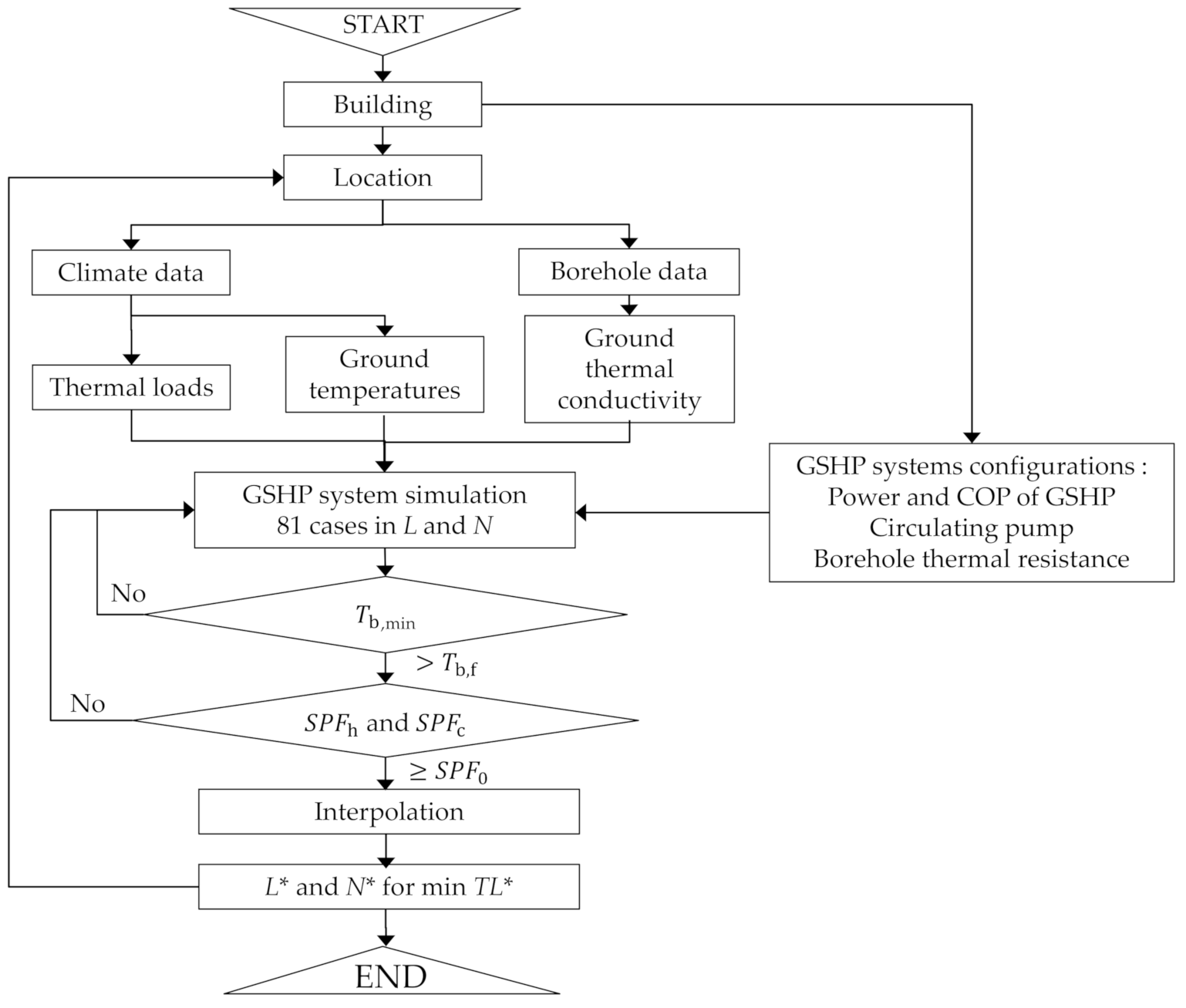
2.1. Simulation Approach for Determination of Total Lengths of Multiple Borehole Heat Exchangers (BHEs)

The simulation methodology used to evaluate the performance efficiency of GSHP systems has been developed in the literature [30,31]. It consists of cyclic calculations of the temperatures of (1) the soil surrounding the BHEs; (2) the heat transfer fluids in the U-tubes; and (3) the fluids entering and exiting the heat pump. The calculation was performed according to hourly thermal loads, resulting in the most realistic solutions as the highest level in the text [14]. First, all configurations of the thermal demands, geology, and system facility were assigned to each cell in various locations. In particular, ground thermal conductivity was input at the same depth with the length L of BHEs as in the previous estimates [32], as shown below. At each time step, the changes in soil temperature around each BHE were estimated as the superposition of temperature changes according to all hourly thermal pulses not only at the targeted BHE itself but also from all other BHEs. The algorithm applied the heat transfer theory of an infinite cylindrical source for the targeted BHE itself and the theory of an infinite line source for other BHEs for fast calculation with sufficient accuracy. The calculations based on the infinite source theory were modified by correction factors for finite heat sources such as BHEs in actuality. The targeted BHE changed in order, resulting in the calculation of soil temperature changes around all BHEs.
Next, the heat transfer rate between the fluids and the soils was calculated from differences in their temperatures with respect to the borehole thermal resistance. The calculation of the borehole thermal resistance is divided into analytic solutions and 2D/3D numerical simulation [33,34,35]. In this study, the borehole thermal resistance was calculated by using the 2D boundary element method for the steady temperature differences between fluids and borehole surfaces, considering circulating fluid properties, U-tube materials and its geometry, and as well as grout materials [30]. The temperatures of the fluids at the shank of the outlet U-tube were calculated from the temperatures of the fluids at the shank of the inlet U-tube considering the heat transfer rates between the fluids and the surrounding soils and the thermal capacity within the BHE. The electricity consumption of the GSHP was calculated at each time step by using a relation between the coefficient of performance COP of the heat pump and the temperature of the fluid flowing into the heat pump. The temperatures of fluids flowing out of the heat pump changed after heat extraction for heating or injection for cooling.
The cycle calculation was carried out in each time step. Then, the electricity consumptions of heat pumps and fluid-circulation pumps were summed based on the seasonal performance of GSHP systems for heating and cooling, i.e., SPFh and SPFc, respectively. The simulation was performed under the assumption of long-term operation for convergence in the soil temperature among different conditions of L and N. The interpolation of the results in the final simulation year followed the optimal combination of L* and N*, yielding the lowest TL*(=L* × N*) to satisfy the criteria assigned. The determination of TL* was performed for all cells in the study region. Figure 1 shows a schematic flow of determination of required total lengths of multiple BHEs in this study.

2.2. Geo-Information for Analysis

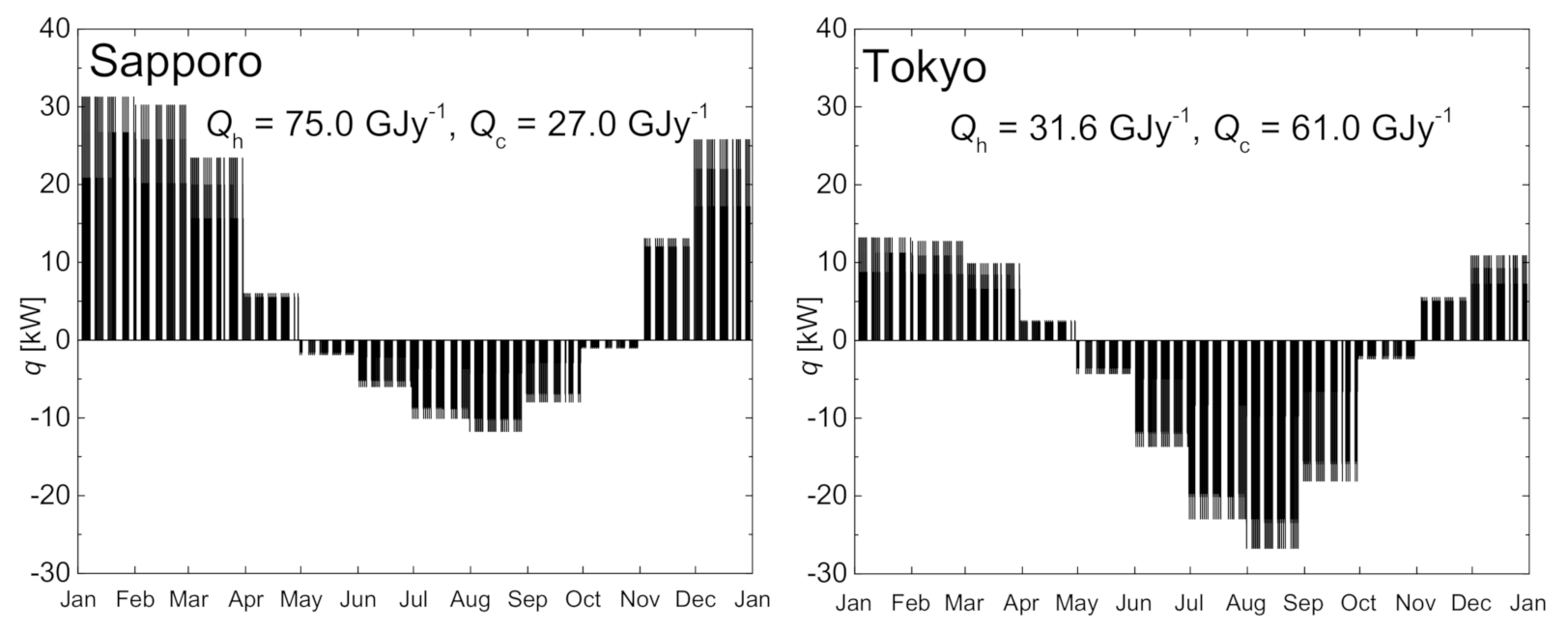
2.2.1. Climate and Thermal Loads

This study was performed to determine TL* on the four main islands of Japan—i.e., Hokkaido, Honshu, Kyushu, and Shikoku—through the simulation approach, as shown in Figure 2a. The mapping was conducted by ArcGIS 10.7.1. The four islands are located along a north-south axis with a length of over 1500 km from 27.0–45.3°N latitude and 128.1–E146.3°E longitude. Thus, the climate conditions are variable. The climate ranges from subarctic on Hokkaido Island to extratropical on Kyushu Island. The climate varies even at the same latitude due to differences in topography, ranging from flat areas near the coast to mountainous areas in the interior. Approximately 70% of the islands feature steep relief due to tectonic and volcanic activities in the Quaternary era, related to Japan’s position as part of the Ring of Fire.
Figure 2a shows the ground elevations in a total of 4156 10-km-gridded cells determined by averaging the digital elevation map [36]. The ground elevations increase toward the middle of each island, with the highest elevation of 2353 m at the center of Honshu Island. Figure 2b,c show the average outside temperatures during heating and cooling, T h ¯ and T c ¯ . GSHP systems were operated for heating at daily outside temperatures lower than 16 °C, and for cooling at temperatures higher than 26 °C. The original temperatures for averaging were obtained from the published weather database [37] for the period during 2000 and 2010, at the nearest meteorological weather station for each cell. This study corrected the outside temperatures for each cell, considering a temperature gradient of –0.006 Km−1. Figure 2b indicates that T h ¯ ranged between <0 °C in most of Hokkaido Island, and >8 °C in the warm and low-elevation areas in the western areas of Honshu, Shikoku, and Kyushu Islands. Figure 2c shows the small range of T c ¯ between 26 and 30 °C, relative to T h ¯ . Figure 2d also indicates the averaged humidity during cooling, R H c ¯ , from the same weather database. R H c ¯ becomes higher in the southern regions than the northern regions. In addition, the climates were more humid near the coasts. Thus, the climate conditions of Japan are variable not only regionally along the north–south direction but also locally according to elevations as well as in the west–east direction.
Figure 2e and f show the annual heating and cooling loads, Qh and Qc, of a two-floor office building with the same total floor area of 300 m2 in each mesh. This floor area is the legal minimum criterion for submitting a construction permit to the government in Japan. These loads in Tokyo were calculated from the practical guide of Japan [38] for room temperatures of 22 °C for heating and 27 °C for cooling with humidity of 50%. The modification factors of Qh and Qc were also summarized for 27 other cities to cover the land in Japan. This study derived relationships for the modification factors with annually averaged temperatures and relative humidity, resulting in Qh and Qc for each cell, as shown in Figure 2e and f. Qh increased from 12 GJy−1 in southern Kyushu Island to 127 GJy−1 in northern Hokkaido Island. The increase is also shown from low coastal elevations to higher interior elevations on each island. The trend in Qc was almost opposite that of Qh, ranging between 1 GJy−1 on Hokkaido Island and 82 GJy−1 on Kyushu Island., Qc was also high along the western areas with low elevations due to the westward anticyclone winds in summer. This study translated Qh and Qc to hourly thermal steps as standard schedules for thermal use, as in the previous study [39]. Figure 3 shows two examples of hourly thermal steps on meshes for northern Sapporo (43.062° N, 141.354° E) and central Tokyo (35.683° N, 139.753° E). Heating demands were dominant in Sapporo while cooling demands were dominant in Tokyo. Figure 2 and Figure 3 indicate that the balance of heating/cooling loads in the building varied among the islands of Japan.

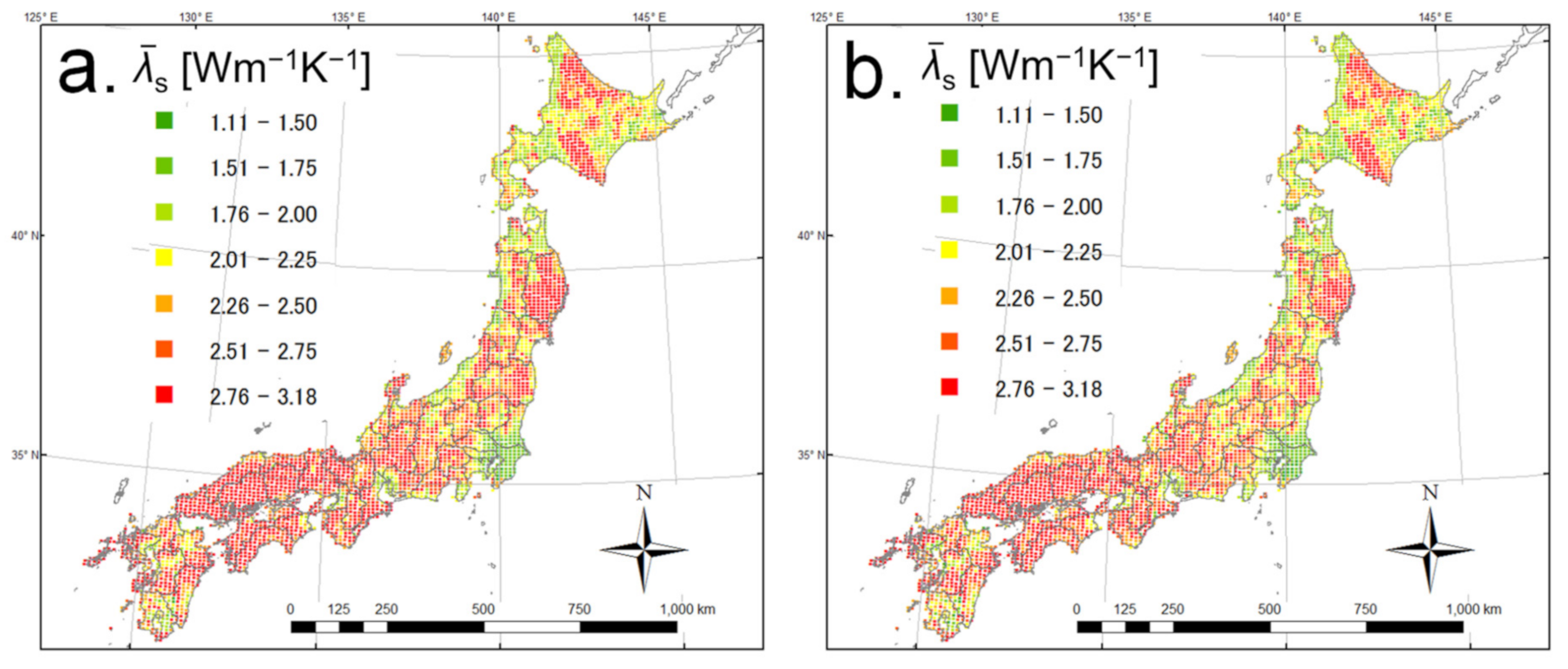
2.2.2. Thermal Properties Underground

The simulation requires assigning three geological properties: ground thermal conductivity, volumetric heat capacity, and initial soil temperature. Ground thermal conductivity λ s ¯ is an overall average of effective thermal conductivity existing in soils in the formation along the BHEs. A previous study [32] provided estimates of λ s ¯ , with a 5-m vertical interval on regular 0.5-km grids over the four main islands by applying the indicator kriging method with 46,515 borehole data points. The estimates were validated at the same locations within situ tests, indicating an average estimation error of less than 0.25 Wm−1K−1. This study converted the estimates for each 10 km gridded cell obtained by the simulation by averaging 0.5 m gridded estimates within each cell, and the averages were interpolated through an inverse distance weighted (IDW) method by using the algorithm in ArcGIS 10.7.1 to cover all cells, including cases in which no borehole data were available.
Figure 4a,b show two example maps of λ s ¯ on the 10-km-gridded meshes at depths of 50 m and 150 m, respectively. We could show the map of λ s ¯ at any depth from 5 to 200 m. λ s ¯ exceeded 2.5 Wm−1K−1 at these two depths in most cells. This was because the soft deposits were <5 m thick on the high relief covering most parts of the islands. However, in cells on the flat plains near the coasts and on the basins among mountains, λ s ¯ was relatively low (<2.0 Wm−1K−1) because the formations consist mainly of unconsolidated soils. Comparison of λ s ¯ at depths of 50 and 150 m reveals that λ s ¯ increased with increasing depth because the main medium changes from soil to rock. The increase was obvious in the high-elevation areas where bedrock becomes more common with increasing depth. On the other hand, λ s ¯ was not clearly different on the flat plains where cities have developed because the unconsolidated deposits are several hundred meters thick in the basin and plains due to the Quaternary deposition in Japan [40].
Volumetric heat capacity was assumed to be constant at 2.5 MJm−3K−1, as an intermediate value for soils and rocks, because of reduced sensitivity of simulation results to this property [41]. The temperature changes in unconsolidated deposits were much less affected by this property than by λ s ¯ . Additionally, the initial soil temperature is as important as λ s ¯ , especially in terms of affecting whether L or N should increase. The profiles were assumed to be first-order linear relations of initial temperature with depth [42]. The thermal performances of BHEs might be affected by groundwater flows, as shown in previous studies [25,43]. In this study, however, the effect of groundwater was assumed to be negligible because the previous simulation study indicated that the averaged Darcy velocity of groundwater was less than 101 m/y on a scale of 10 km [44]. The velocity was evaluated as a threshold for actual effects of groundwater in a residence or in small buildings with limited thermal loads [45]. The intercept of the linear relation of temperature with depth was assigned to be 1 K larger than the annual average outside temperature for each cell. The gradients toward the depth were also locally variable for each cell, depending on the heat fluxes from the interior. However, this regional study assumed a constant value of 0.03 Km−1 in all cells as an average across Japan [46].

2.3. System Configurations and Performance Target

This study assumed that the GSHP system was equipped with a water-to-water heat pump with an output power of 64 kW for heating and 75 kW for cooling. This study focused on heat extraction by a heat pump and neglected the energy performance for heating/cooling in each office room. In meshes where the maximum heating or cooling pulse exceeded the output power, another heat pump was also installed. The relation of the COP of the heat pump was simply assumed to be a linear function of the hourly temperatures of fluids entering the heat pump. The parameters of the relations, i.e., the slopes and intercepts, varied with respect to heating and cooling; the intercepts for cooling and heating were 3.7 and 9.0, respectively. The gradients for cooling and heating were 0.10 °C−1 and −0.16 °C−1, respectively. These values were obtained from laboratory test data of a commercial GSHP product in the product company catalog. For example, when the entering temperature was −5 °C in a heating time step and 38 °C in a cooling time step, the COPs of the heat pump were calculated simply at 3.2 and 2.9, respectively. The electricity consumption of the heat pump was calculated by dividing the thermal loads by the COP in each time step. The total electricity consumption by pumps for circulating fluids at a flow rate of 15 L/min in each BHE was assumed to be constant at 1 kW. The seasonal performance factors, i.e., SPFh for heating and SPFc for cooling, were calculated by dividing the total load by the total electricity consumption during heating and cooling, respectively.
The configurations of BHE (except for L and N of the BHEs) were assumed to be the same, as is usual in the practice of Japan. Each BHE was assumed to consist of a double 32A high-density polyethylene U-tube buried in a borehole with a diameter of 147 mm. The grout materials were also assumed to be silica sands as usual in Japan. The effective thermal conductivity was assigned at 1.5 Wm−1K−1 as the value for the ratio of silica sand over cement weight of 50% [47]. The multiple BHEs were arranged in regular 3-m grids under the assumption of a square building site with dimensions of 15 × 15 m2. The pipes for circulating fluids were connected in parallel among multiple BHEs, so the thermal pulse in each BHE was the same, with a ratio of the total thermal pulse over the BHE number N. This study assumed that L ranged from 40 to 200 m with an interval of 20 m (nine cases) and that N ranged from one to nine (nine cases), resulting in a total of 81 combinations of L and N. The 5-year system operation simulation was conducted for each combination by repeating the heating/cooling thermal loads to achieve sufficient convergence of the maximum and minimum soil temperatures. Although after the 5-year calculation, the temperatures continued to change, as shown in the previous study [48], this study assumed sufficient convergence to be within 1K, corresponding to the situation that the change of COP was limited to within 0.2 (5% for target SPF0 = 4.0). This study calculated SPFh and SPFc from the electricity consumption values of heat pumps and circulating pumps in the final year.
The lowest TL* in each cell required one necessary condition to be satisfied, and another performance condition was determined. The necessary condition was that the temperatures of the fluids must be higher than the freezing point Tb,f of tap water at 0 °C in the warm areas ( T h ¯ > 8 °C in Figure 2b) and higher than the freezing point of antifreeze consisting of 20% ethylene glycol in the cold areas ( T h ¯ ≤ 8 °C). The targeted performance condition stipulated that both SPFh and SPFc must be higher than the target SPF0 value of 4.0, considering that SPFh was recommended to be at least 4.0 for new buildings in the European Norm EN15450. The results of minimum fluid temperatures Tb,min, SPFh and SPFc were interpolated to determine the optimal combination of L* and N* as the lowest total length TL* for sustainable use and target performance.

2.4. Comparison between Simulated and Conventional Methods

This study compared simulated TL* with the TL determined via the conventional method of Japan [13]. The conventional TL0 was determined by dividing the maximum thermal pulse qmax by the specific heat extraction and modified COP. The specific heat extraction rate was assigned a value ranging from 50 to 80 Wm−1 according to λ s ¯ and the total operation time of the system [12,13]. The modified COP was calculated at COPh/(COPhCOPc) for COPh = 3.5 in heating or at COPc/(COPc + 1) for COPc = 4.0 in cooling. In this study, the ratio TL*/TL0 was calculated for each cell, and the results indicate the cost-effectiveness of determining TL* by the simulation approach when TL*/TL0 < 1.
Figure 5 shows two examples of interpolated contours for simulated Tb,min, SPFh, and SPFc for all 81 cases of L and N for the thermal loads of the cities of Sapporo and Tokyo in Figure 3. Table 1 summarizes the climate conditions and the optimization results. All contours were smoothly distributed according to L and N. Tb,min should be higher than Tb,f of –15 °C in Sapporo and 0 °C in Tokyo. The necessary condition was less critical for the determination of L* and N* than for SPFh and SPFc. In Sapporo, L* and N* were 134 m and 2, respectively, for the lowest TL* of 268 m in order to satisfy SPFh with the target performance (4.0). However, in Tokyo, L* and N* were 90 m and 3, respectively, resulting in TL* = 270 m for an SPFc value greater than 4.0. Comparing the results for the two cities shows that the TL* was almost the same, but that the optimal combination of L* and N* was different. Both cities are on flat plains, and the ground thermal conductivity of unconsolidated sediments was less than 2 W−1mK−1. In Sapporo city, where the heating demand was dominant, the L* of each BHE was longer in order to enhance the heat extraction in the deep zones with higher ground temperatures. On the other hand, in Tokyo, where the cooling demand was dominant, multiple BHEs were required; thus, the L of each BHE was shorter, but the N was larger than that in Sapporo city. The conventional TL0 was calculated at 634 and 559 m, respectively. The ratio TL*/TL0 in both cities was less than 0.5, indicating the potential reduction of the capital costs versus those of conventional design.

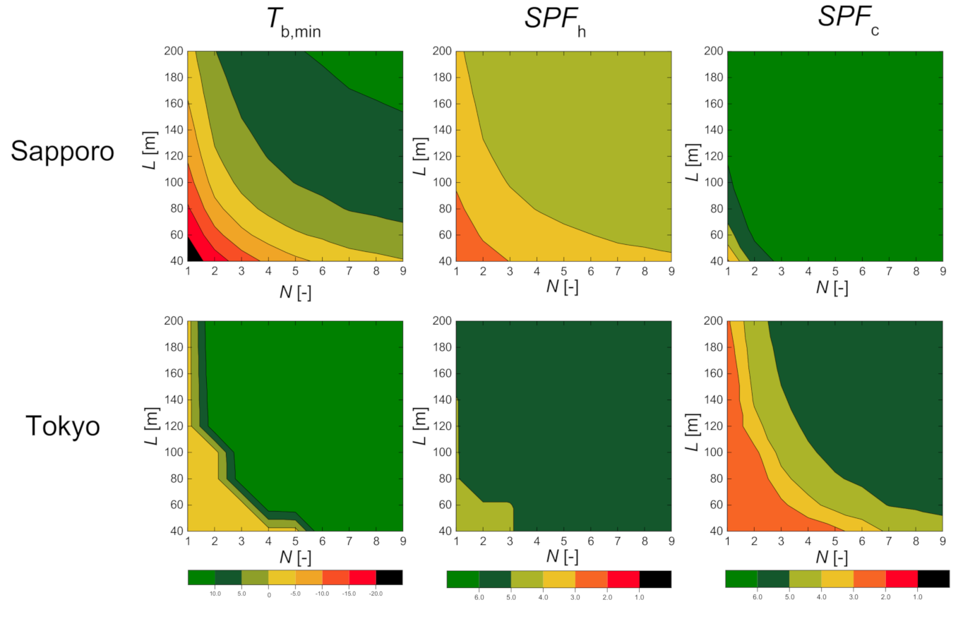
3. Results and Discussion

Figure 6 shows simulation results for a total of 4059 10-km-gridded cells across the four islands of Japan: (a) L*, (b) N*, (c) TL*, and (d) TL*/TL0. There are 97 uncolored meshes in northern and eastern Hokkaido Island for which the heating demands were too high for the systems to satisfy the target performance with a maximum TL of 1800 m (L = 200 m and N = 9) in this study. Figure 7 shows histograms of (a) L*, (b) N*, and (c) TL*, along with their statistical values (maximum, minimum, and average).
In Figure 6a, L* primarily ranges between 60 and 190 m and exhibits an average of 128 m. The simulated L* increases toward the north and the interior of islands, similar to Qh, as shown in Figure 2e. Considering the increase in temperature with increasing depth, L* should increase for efficiency of the systems in cold areas where heating demands are dominant. However, in most cells, L* was not equal to the maximum (200 m in this study), as N was restricted to integer values. Figure 7a shows that L* was distributed almost uniformly, especially between 60 and 190 m, indicating the wide range of L* across the land of Japan.
In Figure 6b and Figure 7b, N* ranged between one and nine, but most systems required a value no greater than three. This indicated that the cooling demands were insufficient to determine variable N for the relatively small buildings for this study. In particular, a single BHE (N* = 1) was sufficient in the northern area of Honshu Island from 35° N to 40° N in latitude. Multiple BHEs were needed in other areas, and N* increased in the southern areas to address increasing cooling demands. N* also increased in the northern area of Hokkaido Island in order to address the large heating demands. These results indicate that the regional trend of a combination of L* and N* was dependent on the climate conditions in Japan. The cells with N*greater than four were observed not only in northern Hokkaido and southern Kyushu Islands but also locally in flat plains near the eastern coasts of Honshu Island—for example, around Tokyo City—due to climate and geological conditions, relatively large cooling demands on the eastern coasts, and a gentle increase in ground thermal conductivity in the soft formation. On the local scale (for example, among adjacent cells), L* and N* were also variable because of differences in ground thermal conductivity. In typical cells where the main materials of the formations changed from soft soils on the flat plains to solid rocks in the mountains, L* and N* suddenly changed. Therefore, the optimal combinations of L* and N* were dependent not only on the regional climate but also on the local geology.
In Figure 6c, as a result of L* × N*, TL* ranged widely between 78 and 1782 m, with an average of 273 m, but was less than 400 m in most cells except throughout most of Hokkaido Island (which has large heating demands) and in some parts of Kyushu Island (which has large cooling demands). Figure 7c also shows that TL* was distributed approximately as a log-standard distribution. The simulation study found that TL* values over 100 m were required, but TL* values were less than 400 m in 3453 cells, i.e., 85% of the cells across the four islands of Japan, despite the variability in L* and N* depending on the climatic and geological conditions. The limited TL* across the land also indicates the feasibility of GSHP systems in this country.
Figure 6d and Figure 7d show TL*/TL0 as a comparison of the TL values determined via the simulation and conventional methods. The TL*/TL0 ratio was 0.5 or less in 69% of the cells (2817 cells), mainly excepting those in northern Hokkaido Island, for the assumed building. This means that the total length of multiple BHEs could be reduced by half or more in most areas of Japan, indicating the potential cost-effectiveness of the simulation approach compared with the conventional approach. It is expected that the simulation-based design method would induce the market growth of the systems and contribute to a reduction in CO2 emissions in buildings of Japan. On Hokkaido Island, on the other hand, the TL*/TL0 ratio was greater than 0.5, especially in the western part, where it was approximately 1.0 or more. In such cold areas with large heating demands, TL* became greater than TL0 in order to satisfy the target performance (SPFh > 4). This also means that the conventional method was limited and that the simulation approach was required to design a GSHP system to obtain such target performance under large thermal demands.
Figure 8 shows plots of the simulated TL* with the simulation parameters Qh, Qc and λ s ¯ . The data in these three plots are scattered, indicating that TL* was dependent not on a single parameter but upon all three. Comparison of the three parameters in the plots revealed that TL* shows a relatively clear relation with Qh in Figure 8a. The relation was assumed to be a second-order polynomial function, with a lower bound of approximately 150 m for Qh between 40 and 70 GJy−1. TL* increased almost linearly with Qh when Qh was over 70 GJy−1 and reached a maximum at 1782 m. TL* also increased as Qh decreased in the range of Qh less than 40 GJy−1 because another Qc increased in the southern areas. The relation of Qc in Figure 8b was also parabolic, similar to Qh, but was less clear. In particular, TL* was more scattered at low Qc values than at low Qh values. TL* also increased with increasing Qc when Qc exceeded 50 GJy−1, but the increase was limited to less than 500 m at a Qc value of 80 GJy−1. Compared with Qh and Qc, λ s ¯ was not obviously related to TL*, as the plots in Figure 8c resemble a cloud. The lower sensitivity of λ s ¯ versus those of Qh and Qc results because λ s ¯ increased only in the mountainous areas where bedrock was more common in the deep zones, in the mountains, λ s ¯ was still large at approximately 2.5 Wm−1K−1 even at shallow depths, as shown in Figure 4a. In the plains with low λ s ¯ , the increases in λ s ¯ were not observed because of the substantial thickness of the soft soil sediments. This indicates that TL* was more affected by horizontal variability of Qh and Qc in different meshes than λ s ¯ . However, when the target scale is smaller than 10 km, for example, 500 m [49] in the previous simulation of BHE sizes in a residence, the relationship of TL* with λ s ¯ would be more obviously obtained.
Finally, the uncertainty in this simulation study is discussed. First, this study demonstrated the nation-scale analysis in the same building and system facility, which are no less significant than climate and geology. Especially in larger buildings, more simulation periods were needed to obtain the convergence of the temperature calculations [48]. The sensitivity analysis in Figure 8 shows that the ground thermal conductivity played a less significant role in TL* than heating/cooling demands on the scale of 10-km grids. However, the sensitivity increases at smaller scales, such as 1-km or smaller grids. In addition, the effect of groundwater flow could enhance the performance through the advection effect [25,44]. We assumed that the effect was negligible on a scale of 10 km. However, the effect should be considered on smaller scales in the simulation by using the developed algorithms [50] or other numerical simulation approaches. This study also assumed that the gradient of the initial ground temperature was constant at the average of Japan. However, the simulation results indicated that the gradient was also crucial in determining an optimal combination of L* and N* while considering a balance of heating/cooling demands. It is necessary in our future study to estimate the gradients of ground temperatures on the national scale—for example, by deriving the relations of other parameters, including the upward heat fluxes from the interior, the sedimentary structures, and groundwater flow velocity. The required TL* would change according to the assumptions of the building specifications such as the floor area, the GSHP system configurations, circuit arrangement of BHEs, and the target for the determination of BHEs. For example, simulation for a variety of building sizes not only 300 m2 but also 500, 2000, and 10,000 m2 in a floor area, is needed to evaluate the nation-scale contribution of GSHP systems for energy conservation and CO2 emission reduction. However, the simulation for floor areas greater than 300 m2 would require a simulation cycle of more than five years. Additionally, the circuit arrangement of BHEs should be optimized to be the most efficient in terms of temperatures in circulating fluids. A sensitivity analysis study of different configurations is also required in the future. Although several limitations and assumptions remain in this study, it was concluded that the simulation approach was economically effective in determining the total lengths of multiple BHEs in buildings. The simulation approach has the potential to contribute to expanding the market of GSHP systems and to reducing CO2 emissions from thermal uses in buildings by estimating the economically reasonable capital costs through the lowest total lengths while considering realistic conditions of climate and geology.

4. Conclusions

This study performed a numerical simulation of the required total length TL* for multiple BHEs on the national scale in Japan. The simulation was performed for a standard building with a total area of 300 m2 in 4059 10-km-gridded meshes with different hourly heating/cooling loads and ground thermal conductivity values. The simulation of the 5-year operation of GSHP systems was performed for each mesh with 81 different conditions of individual length L and number N of BHEs. The results of minimum temperatures of fluids in U-tubes Tf, min and seasonal performance factors SPFh and SPFc for heating/cooling were interpolated and optimized by coupling the required individual length and total number, L* × N*, in all cells to satisfy their criteria. The simulated TL* values were compared with the TL* values determined by the conventional method. The sensitivity of TL* to heating/cooling demands and ground thermal conductivity is shown. The results are summarized below.
(1) The simulation-determined L* ranged mainly between 60 and 190 m and exhibited an average of 128 m. The length increased toward the north and the island’s interior as the heating loads increased because of the increasing ground temperatures with depth. N* reached values of no more than three for the assumed small building. L* and N* were regionally variable depending on the climate and varied locally among adjacent cells due to geological differences.
(2) As a result of L* × N*, TL* ranged widely between 78 and 1782 m (with an average of 273 m), but in most grid cells, it was less than 400 m, except for Hokkaido Island in the north and the southern part of Kyushu Island. TL* did not change despite variations in climate and geology. This study highlighted the effectiveness of the simulation approach for the determination of multiple BHEs because the simulated TL* was half or less of the TL0 obtained by the conventional method in approximately 80% of the cells except for northern Hokkaido Island, indicating the feasibility of the systems in Japan and the potential contribution to reduction in CO2 emissions by thermal uses in such buildings. However, in northern areas with high thermal loads, TL* was greater than the TL0 obtained by the conventional method to satisfy the target performance. This also highlights the importance of the simulation approach for the design of GSHP systems to achieve the target performance.
(3) TL* shows a second-order polynomial relationship with the heating and cooling demands. The relation is more clearly shown for heating than for cooling for the assumed building. The plots of TL*with respect to the ground thermal conductivity were scattered in a cloud, indicating an unclear relationship. This was because increases in the geological properties were primarily observed in the mountainous areas where the values were generally high, not in the flat plains with thick and soft sediments.

Author Contributions

Conceptualization, Data Curation, Methodology, Formal Analysis, Visualization and Writing-Original Draft Preparation, Yoshitaka Sakata; Methodology and Validation, Takao Katsura; Conceptualization, Funding Acquisition, Resources, and Supervision, Katsunori Nagano. All authors have read and agreed to the published version of the manuscript.

Funding

This research was funded by the project “Renewable energy heat utilization technology development,” commissioned by the Japanese national agency New Energy and Industrial Technology Development Organization (NEDO).

Institutional Review Board Statement

Not applicable.

Informed Consent Statement

Not applicable.

Data Availability Statement

The data presented in this study are available on request from the corresponding author. The data are not publicly available due to privacy reasons.

Acknowledgments

The water-well data for analysis were provided by the Ministry of Land, Infrastructure, Transport and Tourism of Japan and the National Institute of Advanced Industrial Science and Technology (AIST).

Conflicts of Interest

The authors declare no conflict of interest.

References

  1. IEA Tracking Buildings 2020 Heating and Cooling. 2020. Available online: https://www.iea.org/reports/tracking-buildings-2020/ (accessed on 10 October 2019).
  2. Kavanaugh, S.; Rafferty, K. Geothermal Heating and Cooling; ASHRAE: Atlanta, GA, USA, 2014; pp. 1–15. [Google Scholar]
  3. Self, S.J.; Reddy, B.V.; Rosen, M.A. Geothermal heat pump systems: Status review and comparison with other heating options. Appl. Energy 2013, 101, 341–348. [Google Scholar] [CrossRef]
  4. Sarubu, I.; Sebarchievici, C. General review of ground-source heat pump systems for heating and cooling of buildings. Energy Build. 2014, 70, 441–454. [Google Scholar] [CrossRef]
  5. De Swardt, C.A.; Meyer, J.P. A performance comparison between an air-source and a ground-source reversible heat pump. Int. J. Energy Res. 2001, 25, 899–910. [Google Scholar] [CrossRef]
  6. Schiel, K.; Baume, O.; Caruso, G.; Leopold, U. GIS-based modelling of shallow geothermal energy potential for CO2 emission mitigation in urban areas. Renew. Energy 2016, 86, 1023–1036. [Google Scholar] [CrossRef]
  7. Lund, J.W.; Boyd, T.L. Direct utilization of geothermal energy 2015 worldwide review. Geothermics 2016, 60, 66–93. [Google Scholar] [CrossRef]
  8. FY2018 Report of Shallow Geothermal Energy Utilization in Japan. Available online: https://www.env.go.jp/press/files/jp/111221.pdf (accessed on 10 March 2020).
  9. Sanner, B.; Karytsas, C.; Mendrinos, D.; Rybachc, L. Current status of ground source heat pumps and underground thermal energy storage in Europe. Geothermics 2003, 32, 579–588. [Google Scholar] [CrossRef]
  10. ASHRAE. Chapter 35 Geothermal energy. In 2019 ASHRAE Handbook; ASHRAE: Atlanta, GA, USA, 2019; pp. 35.1–35.51. [Google Scholar]
  11. Closed-Loop Vertical Borehole Design, Installation & Materials Standards. Available online: https://www.gshp.org.uk/ (accessed on 20 September 2019).
  12. VDI Part 2 Thermal use of the ground. Ground source heat pump systems. In VDI Richtlinien 4640; VDI: Berlin, Germany, 2000; pp. 15–28. [Google Scholar]
  13. Takasugi, S.; Takeshima, J.; Uchida, Y.; Nakagawa, S. Planning and design of ground source heat pump systems In Construction Guide of Ground Source Heat Pump Systems; Ohm-sha: Tokyo, Japan, 2014; pp. 16–37. [Google Scholar]
  14. Spitler, J.; Bernier, M. Vertical borehole ground heat exchanger design methods In Advances in Ground Source Heat Pump Systems; Elsevier: Duxford, UK, 2016; pp. 29–61. [Google Scholar]
  15. Luo, J.; Rohn, J.; Bayer, M.; Priess, A. Thermal performance and economic evaluation of double U-tube borehole heat exchanger with three different borehole diameters. Energy Build. 2013, 42, 69–75. [Google Scholar] [CrossRef]
  16. GLHEPro 5.0. 2016. Available online: https://igshpa.org/software/ (accessed on 10 March 2020).
  17. Earth Energy Designer (EED) v3.2. 2015. Available online: https://www.buildingphysics.com/manuals/EED3.pdf (accessed on 10 March 2020).
  18. Diersch, H.J.G.; Bauer, D.; Heidemann, W.; Rühaak, W.; Schätzl, P. Finite element modeling of borehole heat exchanger systems. Part 1. Fundamentals. Comput. Geosci. 2010, 37, 1122–1135. [Google Scholar] [CrossRef]
  19. Śliwa, T.; Gołaś, A.; Wołoszyn, J.; Gonet, A. Numerical model of borehole heat exchanger in Ansys CFX software. Arch. Min. Sci. 2012, 57, 375–390. [Google Scholar]
  20. Retkowski, W.; Ziefle, G.; Thöming, J. Evaluation of different heat extraction strategies for shallow vertical ground-source heat pump systems. Appl. Energy 2015, 149, 259–271. [Google Scholar] [CrossRef]
  21. Montagud, C.; Corberán, J.M.; Montero, Á. In situ optimization methodology for the water circulation pumps frequency of ground source heat pump systems. Energy Build. 2014, 68, 42–53. [Google Scholar] [CrossRef]
  22. Wu, W.; You, T.; Wang, B.; Shi, W.; Li, W. Simulation of a combined heating, cooling and domestic hot water system based on ground source absorption heat pump. Appl. Energy 2014, 126, 113–122. [Google Scholar] [CrossRef]
  23. Retkowski, W.; Thöming, J. Thermoeconomic optimization of vertical ground-source heat pump systems through nonlinear integer programming. Appl. Energy 2014, 114, 492–503. [Google Scholar] [CrossRef]
  24. Casasso, A.; Sethi, R. Assessment and mapping of the shallow geothermal potential in the province of Cuneo (Piedmont, NW Italy). Renew. Energy 2017, 102, 306–315. [Google Scholar] [CrossRef]
  25. Ondreka, J.; Rüsgen, M.I.; Stober, I.; Czurda, K. GIS-supported mapping of shallow geothermal potential of representative areas in south-western Germany. Renew. Energy 2007, 32, 2186–2200. [Google Scholar] [CrossRef]
  26. Nam, Y.; Ooka, R. Numerical simulation of ground heat and water transfer for groundwater heat pump system based on real-scale experiment. Energy Build. 2010, 42, 69–75. [Google Scholar] [CrossRef]
  27. Iorio, M.; Carotenuto, A.; Corniello, A.; Di Fraia, S.; Massarotti, N.; Mauro, A.; Somma, R.; Vanoli, L. Low Enthalpy Geothermal Systems in Structural Controlled Areas: A Sustainability Analysis of Geothermal Resource for Heating Plant (The Mondragone Case in Southern Appennines, Italy). Energies 2020, 13, 1237. [Google Scholar] [CrossRef] [Green Version]
  28. Walcha, A.; Mohajerib, N.; Gudmundsson, A.; Scartezzini, J.L. Quantifying the technical geothermal potential from shallow borehole heat exchangers at regional scale. Renew. Energy 2021, 67, 217–224. [Google Scholar] [CrossRef]
  29. Spitler, J.; Bernier, M. Editorial ground source heat pump systems: The first century and beyond. J. HVAC Res. 2011, 17, 891–894. [Google Scholar]
  30. Nagano, K.; Katsura, T.; Takeda, S. Development of a design and performance prediction for the ground source heat pump system. Appl. Therm. Eng. 2006, 26, 1578–1592. [Google Scholar] [CrossRef]
  31. Katsura, T.; Nagano, K.; Takeda, S. Method of calculation of the ground temperature for multiple ground heat exchangers. Appl. Therm. Eng. 2008, 28, 1995–2004. [Google Scholar] [CrossRef]
  32. Sakata, Y.; Katsura, T.; Nagano, K. Estimation of ground thermal conductivity through Indicator kriging: Nation-scale application and vertical Profile analysis in Japan. Geothermics 2020, 88, 101881. [Google Scholar] [CrossRef]
  33. Lamarche, L.; Kajl, S.; Beauchamp, B. A review of methods to evaluate borehole thermal resistances in geothermal heat-pump systems. Geothermics 2010, 39, 187–200. [Google Scholar] [CrossRef]
  34. Zanchini, E.; Jahanbin, A. Effects of the temperature distribution on the thermal resistance of double U-tube borehole heat exchangers. Geothermics 2018, 71, 46–54. [Google Scholar] [CrossRef]
  35. Javed, S.; Spitler, J. Accuracy of borehole thermal resistance calculation methods for grouted single U-tube ground heat exchangers. Appl. Energy 2017, 187, 790–806. [Google Scholar] [CrossRef]
  36. Digital Elevation Mesh. 2008. Available online: https://fgd.gsi.go.jp/download/mapGis.php?tab=dem (accessed on 10 June 2019).
  37. Expanded AMeDAS Weather Data: Standard Year File 2001–2010. 2019. Available online: https://www.metds.co.jp/product/ea/ (accessed on 8 April 2020).
  38. SHASE. Simplified Calculation Methods of Cooling and Heating Loads; SHASE: Tokyo, Japan, 2010; pp. 1–26. [Google Scholar]
  39. TES-FS. 2015. Available online: https://www.hptcj.or.jp/Portals/0/data0/technology/manual/ (accessed on 12 June 2015).
  40. Ito, M.; Kameo, Y.; Satoguchi, F.; Masuda, F.; Hiroki, Y.; Takano, O.; Nakajima, T.; Suzuki, N. Neogene-Quaternary sedimentary successions. In The Geology of Japan; Geological Society of London: London, UK, 2016; pp. 309–338. [Google Scholar]
  41. Chiasson, A.D. Geothermal Heat Pump and Heat Engine Systems; John & Wiley Sons: West Sussex, UK, 2016; pp. 185–186. [Google Scholar]
  42. Domenico, P.A.; Schwartz, F.W. Physical and Chemical Hydrogeology, 2nd ed.; John Wiley & Sons: New York, NY, USA, 1998; pp. 191–214. [Google Scholar]
  43. Chiasson, A.D.; Ree, S.; Spitler, J.D. A preliminary assessment of the effects of ground-water flow on closed-loop ground-source heat pump systems. ASHRAE Trans. 2000, 106, 380–393. [Google Scholar]
  44. Sakata, Y.; Katsura, T.; Nagano, K.; Marui, A. Nation-Scale Evaluation of Required Borehole Heat Exchangers Considering Advection Effects of Groundwater Flow in Japan; IAH Congress: Malaga, Spain, 2019. [Google Scholar]
  45. Sakata, Y.; Katsura, T.; Nagano, K. Importance of groundwater flow on life cycle costs of a household ground heat pump system in Japan. Jour JSRAE 2018, 35, 313–324. [Google Scholar]
  46. Arai, T. Hydrology for Regional Analysis; Kokon-shoin: Tokyo, Japan, 2004; pp. 140–161. [Google Scholar]
  47. Fujii, H.; Ishikami, T.; Ohshima, K. Improvement of thermal properties in grouting materials of heat exchange wells in ground-coupled heat pump systems. Shigen-to-Sozai 2003, 119, 403–409. [Google Scholar] [CrossRef] [Green Version]
  48. Lam, Y.; Law, E.; Dworkin, S.B. Characterization of the effects of borehole configuration and interference with long term ground temperature modelling of ground source heat pumps. Appl. Energy 2016, 179, 1032–1047. [Google Scholar]
  49. Sakata, Y.; Katsura, T.; Nagano, K. 500 m-gridded estimation of required lengths for a closed-type borehole heat exchangers in a ground-source heat pump systems. Jour JSCE 2019, 75, I_177–I_183. [Google Scholar]
  50. Katsura, T.; Shoji, Y.; Sakata, Y.; Nagano, K. Method for calculation of ground temperature in scenario involving multiple ground heat exchangers considering groundwater advection. Energy Build. 2020, 220, 110000. [Google Scholar] [CrossRef]
Figure 1. Schematic flow of determination of required total lengths of multiple borehole heat exchangers (BHEs) in this study.
Ijgi 10 00205 g001
Figure 2. Topographical and climate maps of Japan: ground elevations [36] (a), averaged outdoor temperatures [37] during heating (b) and cooling (c), averaged outside humidity (d), and annual thermal loads for heating (e) and cooling (f) in a building of 300 m2. Each cell size is 10 × 10 km2. The thermal loads were estimated by the method of the Society of Heating, Air-Conditioning and Sanitary Engineers of Japan (SHASE) [38].
Ijgi 10 00205 g002
Figure 3. Hourly thermal loads for simulation of cells of Sapporo and Tokyo. Positive and negative values denote heating and cooling, respectively.
Ijgi 10 00205 g003
Figure 4. The 10 km gridded cell estimates of ground thermal conductivity at depths of 50 m (a) and 150 m (b).
Ijgi 10 00205 g004
Figure 5. Simulation results of 5-year ground-source heat pump (GSHP) operation in Sapporo and Tokyo.
Ijgi 10 00205 g005
Figure 6. Simulation results of required length of each BHE L* (a), total number of BHEs N* (b), total length TL* (c), and the reduction ratio compared with conventional total length TL*/TL0 (d).
Ijgi 10 00205 g006
Figure 7. Histograms of analysis results: L* (a), N* (b), TL* (c) and TL*/TL0 (d) for a total of 4059 meshes (all 4156 meshes except 97 meshes without results).
Ijgi 10 00205 g007
Figure 8. Plots of simulated required total lengths of BHEs with heating (a), cooling (b) loads and ground thermal conductivity (c).
Ijgi 10 00205 g008
Table 1. Two examples of simulation results in the cities of Sapporo and Tokyo in Japan.
CitySimulation ConditionsSimulation Results
Qh
[Gjy−1]
Qc
[Gjy−1]
λs
[Wm−1K−1]
L*
[m]
N*
[-]
TL*
[m]
TL0
[m]
TL*/TL0
[-]
Sapporo75.027.01.7913422686340.42
Tokyo31.661.01.709032705590.48
Publisher’s Note: MDPI stays neutral with regard to jurisdictional claims in published maps and institutional affiliations.

