
Edge Detection in 3D Point Clouds Using Digital Images


Laboratory of Photogrammetry, NTUA, 15780 Athens, Greece
*
Author to whom correspondence should be addressed.
ISPRS Int. J. Geo-Inf. 2021, 10(4), 229; https://0-doi-org.brum.beds.ac.uk/10.3390/ijgi10040229
Submission received: 15 February 2021
/
Revised: 24 March 2021
/
Accepted: 1 April 2021
/
Published: 6 April 2021
(This article belongs to the Special Issue Cultural Heritage Mapping and Observation)
Abstract
:This paper presents an effective and semi-automated method for detecting 3D edges in 3D point clouds with the help of high-resolution digital images. The effort aims to contribute towards addressing the unsolved problem of automated production of vector drawings from 3D point clouds of cultural heritage objects. Edges are the simplest primitives to detect in an unorganized point cloud and an algorithm was developed to perform this task. The provided edges are defined and measured on 2D digital images of known orientation, and the algorithm determines the plane defined by the edge on the image and its perspective center. This is accomplished by applying suitable transformations to the image coordinates of the edge points based on the Analytical Geometry relationships and properties of planes in 3D space. This plane inevitably contains the 3D points of the edge in the point cloud. The algorithm then detects and isolates those points which define the edge in the world system. Finally, the goal is to reliably locate the points that describe the desired edge in their true position in the geodetic space, using several constraints. The algorithm is firstly investigated theoretically for its efficiency using simulation data and then assessed under real conditions and under different image orientations and lengths of the edge on the image. The results are presented and evaluated.
1. Introduction
Geometric Documentation of Cultural Heritage is considered a necessary background for all archaeological and architectural studies for the restoration of cultural heritage monuments and objects, as mandated by the Venice Charter Available online: https://www.icomos.org/charters/venice_e.pdf (accessed on 3 April 2021). To this day, this is performed through the production of traditional two-dimensional vector drawings, and it is estimated that these will not be replaced soon. Creating such linear drawings is a time-consuming process for an engineer because it is conducted manually.
The basic steps and considerations for the successful Geometric Documentation of a cultural heritage object are the following. Primarily is the deep understanding of the monument and the consideration of all historical and archaeological data related to it. This implies the correct study and deep understanding and interpretation of the object, especially its structure and construction phases through its history. This is a crucial fact that an engineer must consider before any data acquisition action, as these elements should be reflected to the documentation products. This study must precede all other plans and actions, it should be made in situ and in collaboration with experts with deep knowledge of the monument—preferably the final users. This reconnaissance should clear all details concerning level of detail (LoD), precision, form of final products and—of utmost importance—the users’ needs. In finalizing the deliverables, i.e., general documentation drawings, detail drawings and 3D visualizations, eventually existing general specifications should be adapted to the specific needs of the object. Unfortunately, such general specifications very rarely exist, and consequently each monument should be documented with its own specifications. This is a need which should be addressed in the future.
In recent years, automation has enabled the rapid acquisition of loads of digital data for the documentation of cultural heritage objects, be they immovable or movable, large, or small. These data are characterized by high accuracy and reliability and offer a lot of possibilities to experts for the thorough documentation of cultural heritage objects. However, processing of the acquired data requires expertise, specialized software, powerful hardware and, most importantly, time. On average, the ratio of the required processing time to the time needed for the acquisition of the data is 15:1, based on our extensive experience with complex architectural monuments presenting high level of detail and requiring large-scale surveys.
The need for optimization and automation of the above processes has often been performed using automatic feature extraction in 3D point clouds, a novel research topic in the fields of Image Analysis, Image Processing and Computer Vision that has been studied in recent years [1,2,3,4,5]. However, the various approaches are not competent enough to arrive at a holistic solution, which has long been a major issue in the 3D modeling applications. In general, in the field of image edge extraction, edges are detected based on the boundary between areas of different brightness or texture [6,7,8]. However, the methods used to detect edges in the images cannot be applied to unorganized 3D point clouds, because they obviously have a different structure from images, as an image is a matrix of (i, j) elements, while an unorganized point cloud is an irregularly distributed set of data [2,9]. This variation in their structure results in the unsuitability of edge detection methods used in images and indicates the emergence of edge detection and extraction from unorganized point clouds as an important research issue [2,3,10].
To address the tasks mentioned above, an automated and effective method for detecting edges in unorganized 3D point clouds is developed and proposed, by exploiting the relationship of oriented digital images, thus connecting 2D image coordinates and 3D space. The software was developed in the Jupyter and Spyder environments using various open-source libraries. The programming language is Python, an open-source programming environment.
A desired edge of the object is detected on an image and fed into the algorithm. The plane, to which the desired edge belongs, is created using the properties of Analytical and Projective Geometry. The goal is to select those points of the 3D point cloud which belong to the specific edge in the object. This is achieved by searching for all edges that belong to that identified plane, which is common to the reference system of both the space and the image. The detection of the desired 3D edge is finally accomplished by applying the RANSAC algorithm and sufficient acceptance criteria. The algorithm and the process were implemented in a simulation experiment and in a real-world case study and, finally, are evaluated for their performance. The compatibility of the method in cases of terrestrial and aerial images is expected for the general effectiveness of the algorithm. The conclusions focus on the accuracy with which the edges were detected and the obstacles the algorithm may face in the process of selecting the appropriate edge.
The rest of the article is organized as follows: Section 2 introduces a review of the state of the art methods for edge detection in 3D point clouds; Section 3 outlines the basics of the method developed, with reference to basic notions of Analytical Geometry and Photogrammetry; Section 4 presents our proposed method and algorithm and its development; in Section 5 the implementation on an existing dataset and the necessary fine tuning is presented; while in Section 6 the application of certain acceptance criteria is implemented and evaluated. Finally, in Section 7 some conclusions are drawn, and future work is envisaged.
2. Vectorization of Point Clouds
Edge detection methods are not satisfactory and their detection algorithms neither work automatically, nor provide robust results. At the same time, with advances in aerial and terrestrial laser scanning technology, but also in image-based modeling software, the acquisition of dense point clouds has become increasingly common [11,12]. 3D point clouds are produced using terrestrial laser scanners or LiDAR Sensors and by implementing SfM/MVS procedures with terrestrial images or images taken by UAV or other airborne sensors. Researchers’ efforts to detect edges in those 3D point clouds can be categorized into two groups—direct and indirect methods—depending on the way the desired 3D edges are extracted. Direct methods identify points belonging to the object of interest as the regions with mutual sharp features, using data from sorting through the point cloud itself and categorizing it into clusters. In contrast, indirect methods firstly convert the 3D point cloud into an image, then the selected 2D edges are projected back to the 3D point cloud. In the first category, most of the existing research on extracting edges uses spatial estimation methods considering either statistical [13,14,15] or geometrical methods [16,17,18], or by estimating the normals on sharp edges [19,20,21,22]. The extraction of 3D edges is based on the density and the massiveness, i.e., the size, of the 3D point cloud, but also the object of interest. In Triangular Irregular Networks edges appear on their external or internal borders as outlines of larger edges [10].
Some approaches employ surface models of point data, due to their capability to detect edges of mutual characteristics. Those approaches are used for irregular objects or complex surfaces. Weber et al. [19,20,21] used triangulation for normal estimation by analyzing points enclosed in different neighborhoods. Different techniques use algorithms for the detection of outlines onto objects by sensing changes in the curvature of the surrounding elements to deal with complex contours. Thus, the points that are closest to the change in edges’ curvature are selected and are considered contour points. Methods referring to the Angular Gap [18] have been suggested and produced along with the Point Cloud Library (PCL). The inherent property of an edge here is based on the geometric properties of each query point’s neighborhood and not the point itself.
Based on this principle, Ni et al. [17] present the AGPN algorithm, an automated method validated on complex man-made objects and large-scale urban scenes which includes detecting 3D edges and then tracing feature lines. In the neighborhood of a border element, there is only one curve or flat surface. Close to a folding edge, there are two or more intersecting surfaces. AGPN then combines RANdom SAmple Consensus (RANSAC) [17,23] and angular gap metric to detect edges. In the feature line tracing step, feature lines are traced by a hybrid method based on region growing and model fitting in the detected edges. The pioneers of this principle, Bazazian et al. [10], used a clustering method for edge extraction by analyzing the eigenvalues of the covariance matrix that are defined by each point’s k-nearest neighbors. Hackel et al., in 2016 [24], pointed out the importance of detecting edges along which their orientation changes abruptly using two binary classifiers for each point at first and then for the selected region of points (Markov Random Field).
An interesting approach was presented by Yang and Förstner [16] based on the geometric properties of 3D planes by dividing the point cloud into small rectangular blocks to confirm that there will be up to three planes in every square. This algorithm integrates RANSAC for plane detection and MDL principle searching for the different planes of each block, thus applying a spatial multiplier to connect all neighboring planes belonging to a certain local range of values.
Another group of methods for edge detection is based on segmentation or classification procedures, sometimes supported by machine learning algorithms. Grilli et al. [25] presented a review of point cloud segmentation methods assisted by machine learning algorithms. The review is not fully exhaustive, but it reports many approaches suitable for the geospatial and heritage communities. All methods are grouped into five categories based on their core approach. Ben-Shabat et al. [23] introduced a new graph-based over-segmentation algorithm for 3D point clouds. Their Point Cloud Local Variation (PCLV) algorithm is generic in the sense that it is sensor independent and may be applied to any 3D point cloud data. However, it does not lead to edge extraction suitable for orthogonal projections and does not offer the required accuracy, as it processes rather sparse point clouds. Hu et al. [26] presented an open-source software package (JSENET), which performs edge detection based on point cloud segmentation, while it does not extract the edges and does not use digital images.
3. Methodology
The motivation of the proposed algorithm is to develop an automated solution for straight edge vectorization from 3D point clouds, by exploiting the combination of the cognitive background of Analytical Geometry and Photogrammetry. As already discussed, most edge detection methods define 2D and 3D edges as discontinuities of the geometric properties in the underlying 3D scene and are often associated with abrupt changes in the gray levels on images.
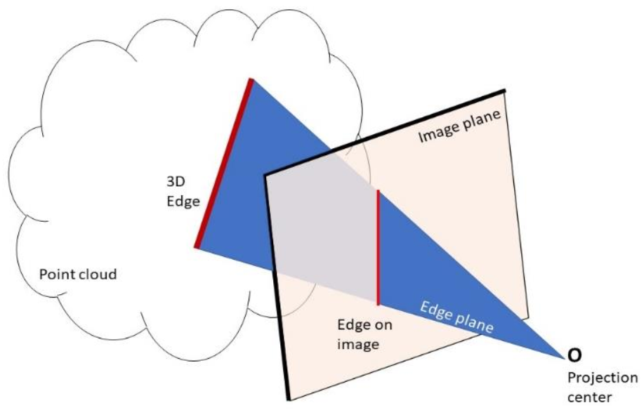
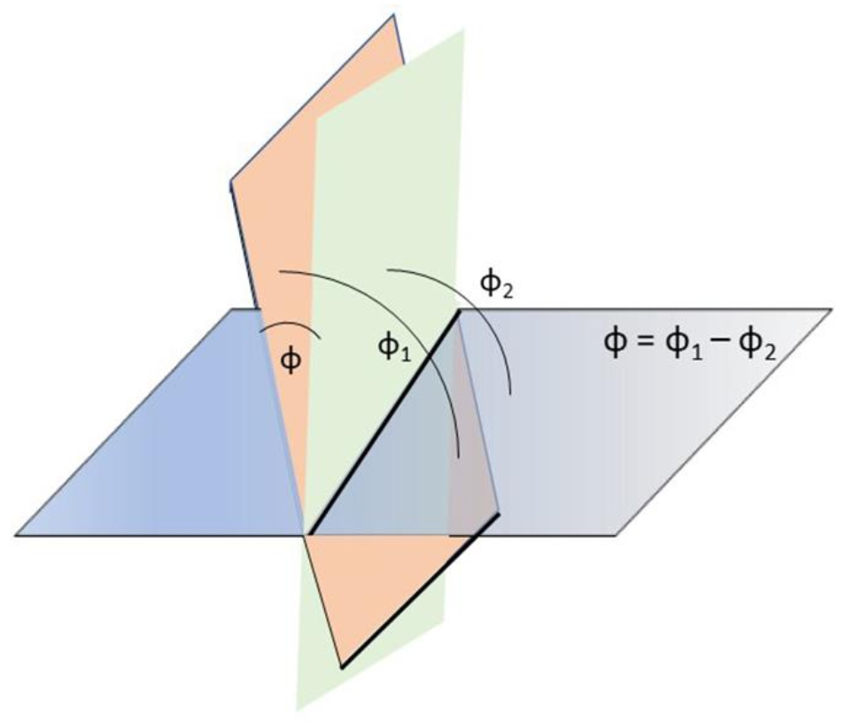
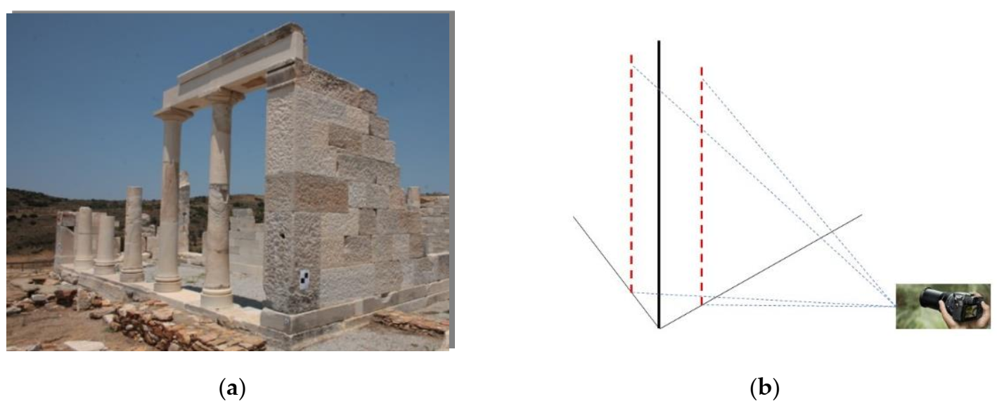
This research attempts to exploit the 3D plane defined by an edge detected in the image and its perspective center (Figure 1). Provided that the exterior orientation of the image is known, and a point cloud, referenced in the same coordinate system, exists, the points of the 3D edge must lie in that plane. Consequently, each 3D line in the point cloud creates a 3D plane, which can be accurately determined using at least two different points belonging to the 3D edge and the 3D space coordinates of the projective center. Obviously, this plane passes through the edge formed on the image.
The necessary parameters to define that plane are the edge on the image, on the one hand, and the exterior orientation parameters of the camera, which include the position of the perspective center O (Xo, Yo, Zo) and the orientation of its axis (ω, φ, κ), on the other. In addition, the intrinsic parameters of the camera should also be known to increase reliability in defining the plane. These parameters include at least the calibrated focal length c, the principal point coordinates (xo, yo) and the radial distortion values. In most photogrammetric applications, the parameters describing the geometry of the camera used, are usually known. It is necessary to identify the two reference systems, image and space, and their relation as well as possible.
It should be remembered that, according to basic Analytical Geometry notions, a plane is defined either (i) by three non-collinear points or (ii) by a point on the plane and the normal vector to it. The general equation of a plane in a rectangular cartesian coordinate system has the following form:
where A, B, C and D are suitable parameters. Two planes ε1 A1x + B1y + C1z + D1 = 0 and ε2 A2x + B2y + C2z + D2 = 0 are identical if:
Ax + By + Cz + D = 0
A1/A2 = B1/B2 = C1/C2 = D1/D2
The main idea of the proposed algorithm is described in the following steps, which will be later elaborated:
- Firstly, an image (or images) of an object is introduced into the algorithm. The image is defined as a matrix of (r, c) pixel values and the image coordinate origin (0,0) is the principal point.
- Then, a desired edge is detected on the image. This may be performed either manually or with one of the numerous edge detection algorithms available. The determination of the edge should be performed with optimal accuracy to reliably determine the plane created by the 2D edge and the projective center of the image in the 3D space with its coordinates (Xo, Yo, Zo).
- Lastly, connecting the image and 3D space reference systems to a common one is an essential step for the developed algorithm. For that purpose, a rigid-body transformation based on the elements of the exterior orientation of the image is applied. In this way the image coordinates are referenced in the 3D coordinate system and thus the plane defined by the 2D edge and the perspective center is defined in the 3D space. It is noted that the available point cloud is also referenced in the same 3D system.
- The 3D points of the edge lie, by definition, on this plane. It remains for the algorithm to seek those points in the 3D point cloud (Figure 1). For that, several criteria are applied to ensure reliable determination of the 3D edge in the point cloud. Those criteria are discussed in the next sections.
The determination of the plane occurs as follows: At least two points are selected on the image edge, e.g., p1 (x1, y1, −c) and p2 (x2, y2, −c), and the line equation can be determined. These coordinates are transformed to the space coordinate system, i.e., that of the point cloud, with the help of the exterior orientation parameters of the image (Equation (3)). This transformation results to P1 (X1, Y1, Z1) and P2 (X2, Y2, Z2), the two points in the space coordinate system, where also the perspective centre O (Xo, Yo, Zo) is known. Those three points (P1, P2 and O) form a plane which profoundly contains the sought edge. The four parameters of the plane can be determined from these three points. All points of the point cloud that satisfy the parametric equation (Equation (1)) of the plane determined belong to this plane. Alternatively, all points of the point cloud with a Euclidean distance from the plane smaller than a preset threshold belong to the plane. At this stage, all outliers are rejected using the RANSAC algorithm and all points that belong to the plane are selected including, of course, the points of the sought edge. Then the algorithm selects the points belonging to the edge from the inliers of the detected plane.
The rigid body transformation makes it possible to connect the vectors of the image with those of 3D space, i.e., the image points (x, y, −c) are related to the points (X, Y, Z) of the selected edge in the world system. The coordinates are transformed according to the rotation and the position of the projective center at the time of the image acquisition, exploiting the known exterior orientation parameters of the image. This transformation is formulated with Equation (3).
where (x, y, −c) are the coordinates of the image points in the image system, R(ω, φ, κ) is the rotation matrix of the image and (Xo, Yo, Zo) the world coordinates of the perspective center. After the implementation of this transformation the plane defined by the edge on the image and the perspective center coincides with the plane defined by the perspective center and the edge in the point cloud (Figure 1).
4. Algorithm Development and Implementation
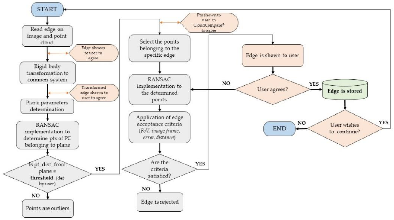
Each step of the developed algorithm was initially investigated for its reliability by creating a representative simulation using artificially created data. In Figure 2, the sequence of the steps of the algorithm are presented in the form of a flowchart.
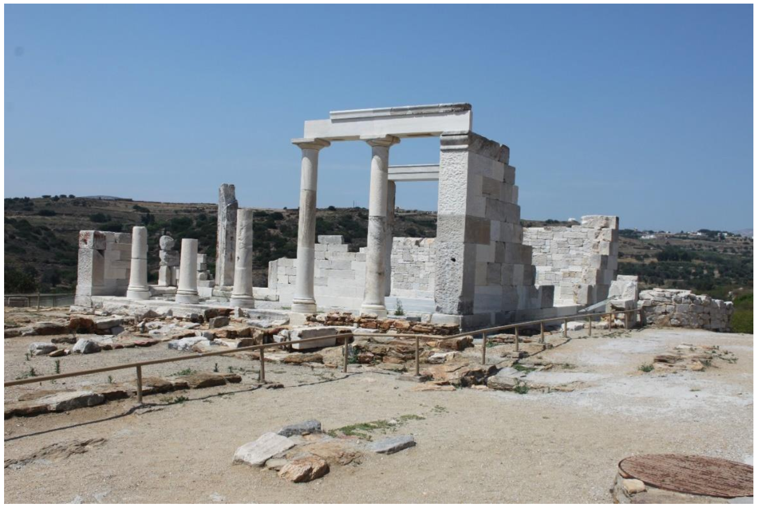
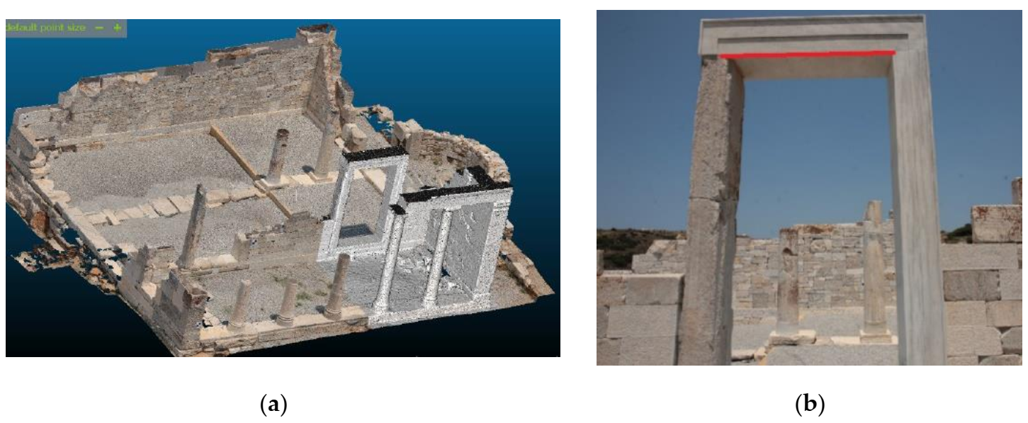
These steps were applied both in a carefully designed simulation created to prove the robustness of the algorithm and in a final practical application in the Temple of Demeter on Naxos island (Figure 3).
The artificial data for the simulation were created using a few, approximately 1000, randomly determined points to build a point cloud within which an edge described by 200 points was present. All points were projected, i.e., imaged, on an image with a simulated camera with known intrinsic and extrinsic parameters. Random Libraries of Python were used for this task. The real-world data consisted of a point cloud consisting of 750,000 points, part of the grater point cloud acquired with a FARO terrestrial laser scanner for the geometric documentation of the Temple of Demeter on Naxos. The point cloud used depicted the front part of the temple as imaged in Figure 3. All images acquired for the geometric documentation of the Temple of Demeter were oriented via an SfM/MVS procedure using the Agisoft Photoscan software v.1.4.
The algorithm starts with the insertion of the 2D edge from an image, depicting the object or part thereof, which is also represented by the existing 3D point cloud. Then, the rigid body transformation described above is applied, considering the principal point image coordinates and the exterior orientation of the image, i.e., the position of its projective center and the orientation of its axis in the same 3D space as the existing point cloud. After that transformation, the points on the image, the perspective center and the point cloud are in the same reference system. Consequently, the plane defined by the points on the image and the perspective center contains, among others of course, the 3D points of the edge from the point cloud. The accurate determination of this plane is crucial, as it is defined by an extremely small part, which is contained in the image space. To determine the points of the point cloud that belong to that plane the RANSAC algorithm is implemented.
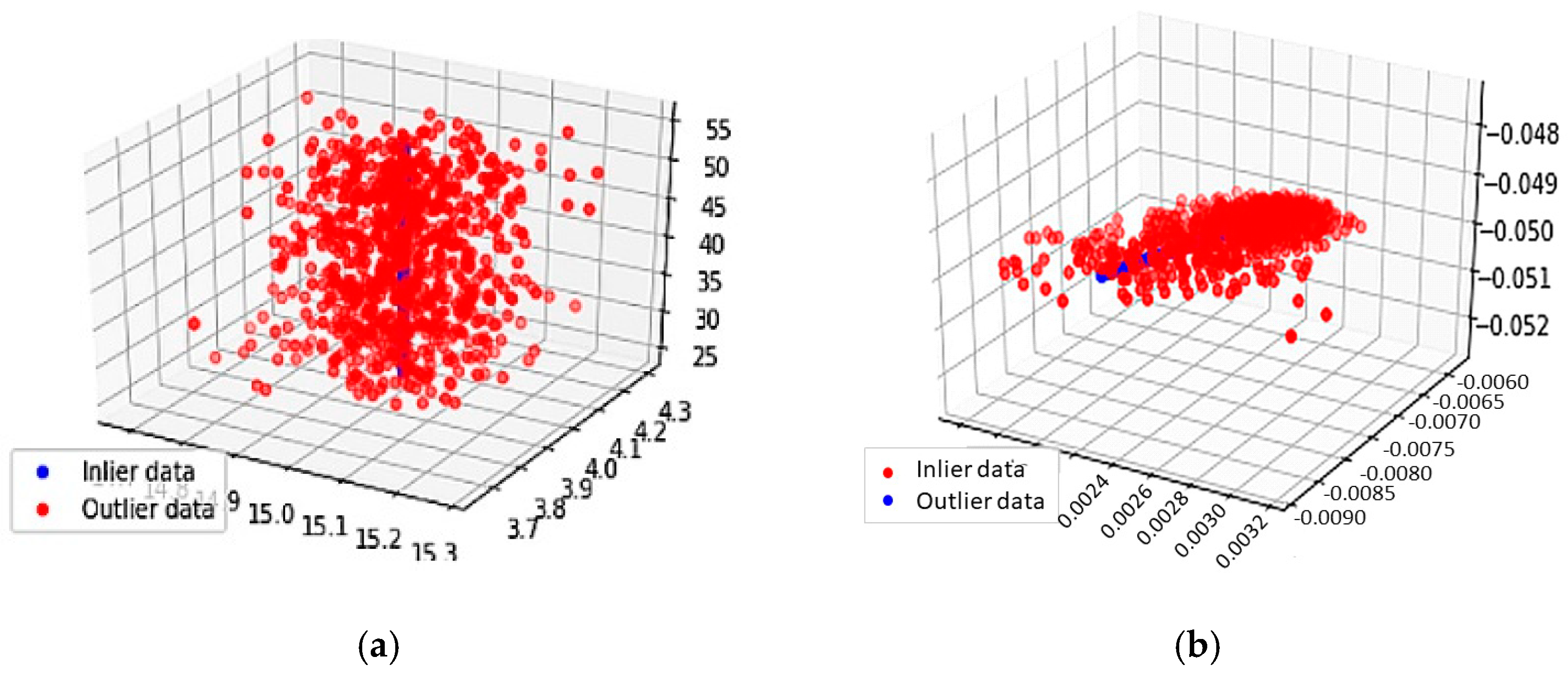
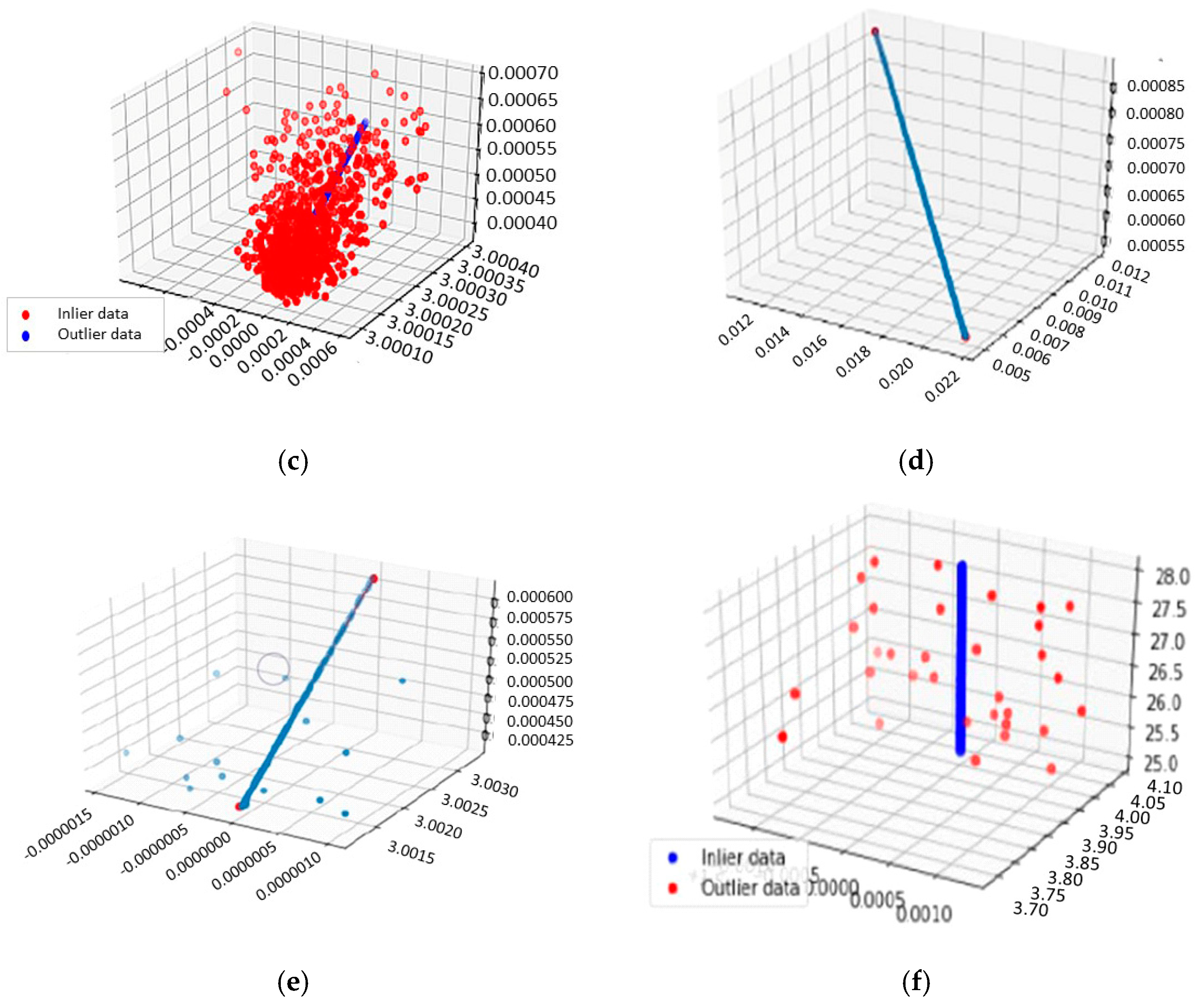
RANSAC extracts shapes by randomly drawing minimal sets from the point data and by constructing corresponding shape primitives. The resulting candidate sets are compared against all points in the dataset to determine how many of the points, called inliers, are well approximated by the primitive, thus forming the greater score of the set. After a given number of trials, the set which approximates the most points is extracted and the algorithm continues with the remaining data [27]. The results of this operating procedure are presented in Figure 4 for the simulation and in Figure 5 for the real-world data resulting in the determination of the 3D edge in the point cloud. In Figure 4a, the original 3D point cloud is displayed, while in Figure 4b the same point cloud is represented as projected on the image. In Figure 4c the resulting point cloud belonging to the determined plane is depicted after the rigid body transformation. Furthermore, Figure 4d presents the segregation of the 2D edge that belongs to the inserted image, while Figure 4d shows the transformed 3D edge in the 3D space. Finally, in Figure 4e, the result of the implementation of RANSAC algorithm to the transformed edge is displayed, with all inliers belonging to the requested edge of the 3D point cloud.
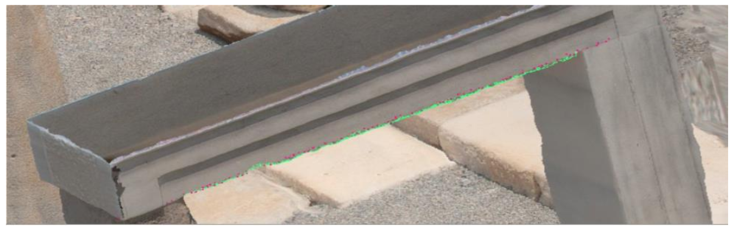
However, the corresponding steps performed using the real data from the Temple of Demeter on Naxos, as shown in Figure 5, result in a summation of points belonging to the determined plane, although they do not necessarily belong only to the wanted 3D edge in space. This discrepancy is dealt with in the second part of the algorithm, where the various acceptance criteria are enforced. The threshold used in RANSAC algorithm for that part of the algorithm depends on the density and the accuracy of the 3D point cloud and is determined by the user.
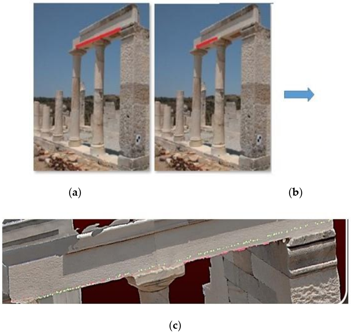
In Figure 5a, the part of the acquired point cloud of the Temple of Demeter composed of 750,000 points is shown. In Figure 5b, the selected 2D edge on one of the available images is depicted. This edge will be sought in the world system of the point cloud. In Figure 5c, the definition of the parameters of the 2D line and acquisition of two characteristic points of the edge is displayed. In Figure 5d, the result of the implementation of the rigid body transformation for that edge is shown. Finally, Figure 5e displays the section of the point cloud with the determined plane depicting with different colors all points belonging to that plane.
5. 3D Edge Detection
The second part of the algorithm applies certain criteria for selecting the right edge among the many linear concentrations of points determined so far in the 3D point cloud (Figure 5e). The acceptance criteria applied on the detected edges are essential for the smooth function of the algorithm and are the following:
- Each investigated edge, when back projected onto the image, should fall within its physical frame, in this case within the 36 × 24 cm2 area, as the images used were taken with a full frame DSLR. If this is not valid the edge is rejected.
- All sections of the non-rejected edges which fall outside the frame of the image should be excluded.
- Each back projected and accepted edge should have similar, i.e., within a threshold value, orientation (inclination) to that of the originally determined edge on the image. If this is not the case, the edge is rejected.
- The edge to be selected should be the one nearest to the projective center, as it was at the time of the image acquisition.
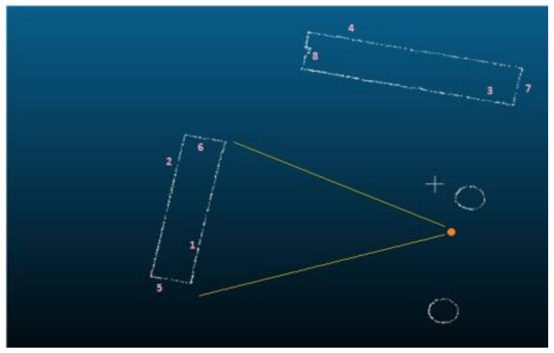
An example is shown in Figure 6, which depicts all edges which are contained in the determined plane (Figure 5e). Of the eight different edges belonging to the requested plane as found by the first part of the algorithm, only #1 is the correct one. The implementation of RANSAC algorithm again uses suitable constraints to obtain that edge and exclude all superfluous edges (#2–8). The yellow lines indicate the field of view (FoV) of the camera. It is obvious that all edges outside the FoV should be excluded. Moreover, the one closest to the perspective center of the camera and having the same or similar orientation with the original one on the image is most likely the sought edge.
As shown in Figure 6, the selection of the appropriate edge among those determined should start by excluding those edges that are back projected outside of the image frame and by keeping only those which fall within the yellow lines, i.e., the FoV of the camera used. The procedure of back projection is performed by applying the collinearity equation, thus returning the edges found by RANSAC to the image coordinate space. The positions and orientations of the back projected edges are compared with those of the edge initially selected. This is achieved via checking if the returned image coordinates (resx, resy) verify the line equation of the initial 2D edge (Equation (4)). If the differences Δx, Δy (Equation (5)) are less than a threshold value defined by the user, the edge is preserved.
Following that, the edge closest to the camera is selected, as it is more likely to be shown in the image than the farthest ones, i.e., edge #2 in Figure 6. Finally, the selected edge is confined inside the image frame and the parts outside are discarded. This is because it is quite difficult to otherwise control the size and position of the detected edge outside the image and it is possible to wrongly accept edges that do not represent the one investigated. If an edge has significant length in the object, it will be detected in parts on adjacent images.
For the experimental implementation of the algorithm and the selection criteria in the specific point cloud of the Temple of Demeter, the total access time for identifying one edge was 25–30 s and the threshold value applied was 1 pixel, or 6 mm, which is the equivalent mean GSD of the images. The threshold value was decided considering the density of the point cloud and the eventual errors added by the interior and exterior orientation of the image.
6. Evaluation of the Results
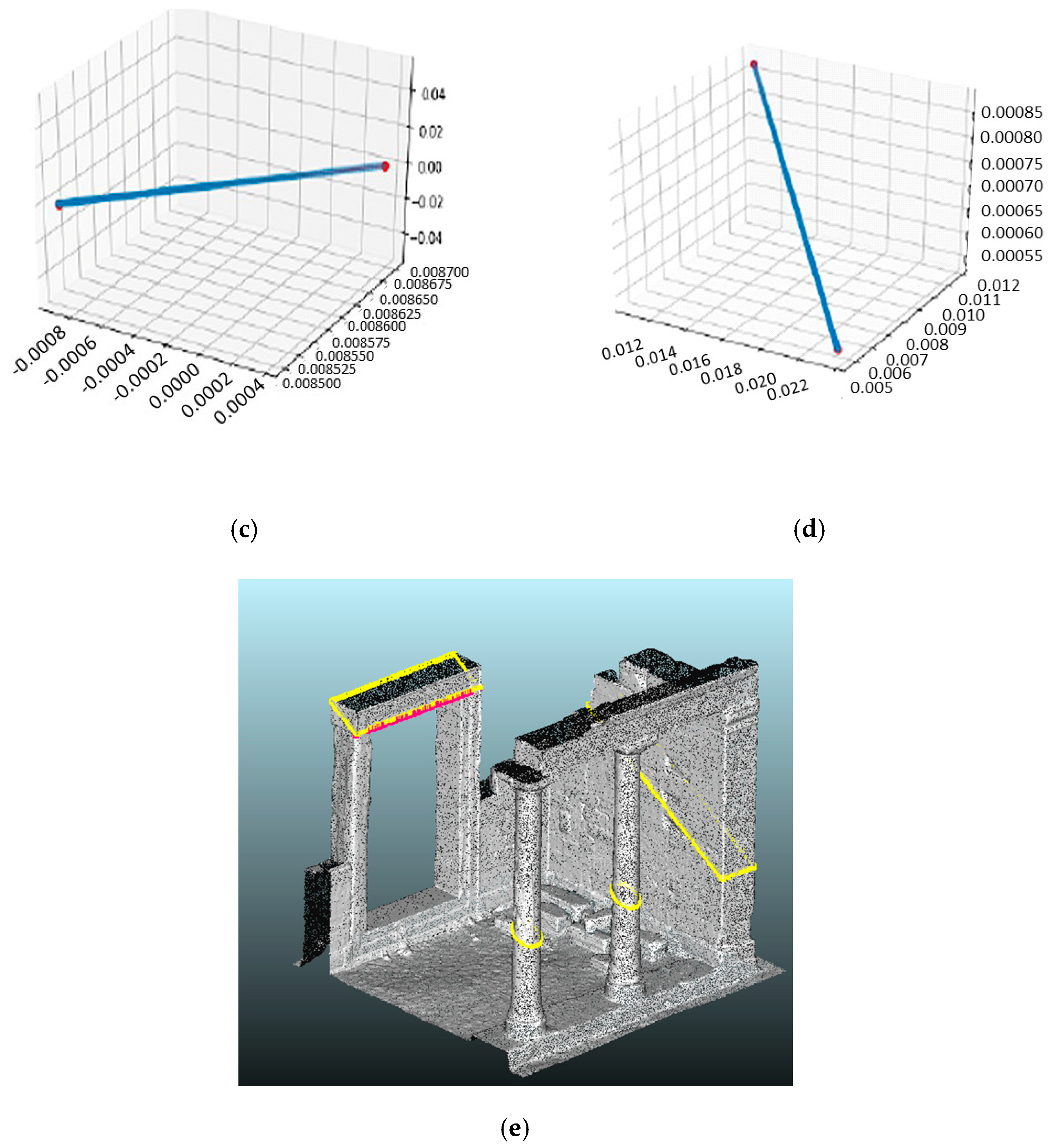
It was considered necessary to study whether significant errors were added to the process during the implementation of the algorithm that would affect the result. Both the plane determination procedures were checked using the error propagation to the functions responsible for the parametrization of the planes and the error was translated both angularly and linearly. The results indicate that the error introduced by the algorithm was calculated to less than 0.3 mm in the world system, for commonplace terrestrial images taken at distances of less than 10 m. The angular error was estimated to be 0.57 cc, which translates to 1.105 × 10⁻⁶ rad, which is considered negligible (Figure 7). Consequently, the determination of the plane based on the image observations is quite stable and is not subject to major variations, proving that the algorithm is robust and powerful. An obvious enhancement for mitigating the error of the back projection on the image would be to include the camera calibration parameters in the algorithm.
The algorithm and the constraints defined, developed, and implemented were assessed under real conditions for different image orientations and edge lengths on the images of the Temple of Demeter. The various results, which contributed to the fine tuning of the algorithm, are presented and evaluated in this section. At the same time, the operation of the algorithm is explained in detail for the success of the edge detection method and assessed under different conditions. The observations made are of particular interest for ensuring the universal applicability of the algorithm in many cases of imported edges and achieving optimal results. The success and usefulness of the algorithm depend mostly on the successful selection of the right 3D edge inside the point cloud among the numerous co-planar 3D edges detected. The implementation of the acceptance conditions or restrictions reassure that the algorithm is working satisfactorily leading to successful localization of the desired edges (Figure 8).
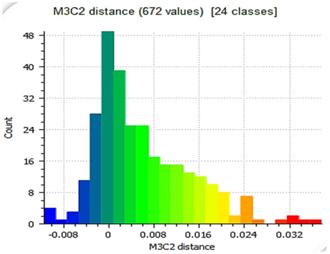
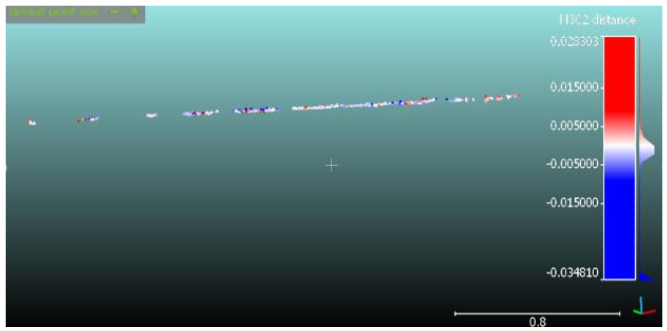
The accuracy of the results achieved is satisfactory, as the image coordinates of the detected edges compare well to the real-world edge when back projected on the image. Specifically, the differences Δx, Δy appear to be less than the desired threshold value, which is set to 1 pixel. Figure 9 presents a histogram which reveals how successfully the two 3D edges, projected in Figure 8, adapt to each other, when compared with the M3C2 tool in CloudCompare®.
Some differences in image coordinates were determined to be larger than the threshold set, i.e., one pixel (Figure 9). This is attributed to the corrosion of the surface of the monument, which is more apparent at the edges. Of course, this deformation is depicted by the laser scanner in the input point cloud.
The effect of not using the exact interior orientation parameters and especially the calibrated focal length on the accuracy of the detected edges was investigated. Obviously, the use of even a slightly different focal length will have an adverse effect on the result, as the shape of the bundle of rays is deformed. This affects the scale of the image as can be seen in Figure 10a, but also leads to erroneous localization of the sought edge (Figure 10b). The focal length varies with the focusing distance, taking its nominal and minimum value at infinity focus, in this case 24 mm. However, as the images were taken at a mean focusing distance of 5 m, the focal length should be set to a higher value. This value was taken from an existing calibration report and was set at 24.5 ± 0.02 mm. The points of the same edge determined using both values of the focal length were located, and the results are shown in Figure 10b, where the erroneous edge is depicted, and Figure 11, where the correct one is compared with the corresponding edge manually detected in the point cloud. It is obvious that the differences of these two edges could adversely affect the resulting 3D edges. The differences of the edge points detected when using the calibrated focal length, as calculated by the M3C2 algorithm in CloudCompare® are less than 5 mm (Figure 11). This means that the calibrated focal length should preferably be used, because the use of the nominal focal length of the camera lens is expected to introduce significant deviations in the edge determination.
A different possible error source investigated concerns edges depicted on images with significant rotations (ω, φ, or κ) at the time of image acquisition. It was proven that if the entire length of the edge is imaged and at a significant length, the algorithm has no problem defining the plane and locating the 3D edge in the point cloud. On the contrary, if a small part of the total edge is depicted or used for the process, the result is directly affected (Figure 12). Robust and more accurate results are obtained if, during the edge selection on the image, those edges are preferred whose image length is as large as possible. In Figure 12c, the white line presents major deviations for the part of the edge which is not described directly in the original image (Figure 12b). The results are extracted successfully, preserving the desired accuracy whether the edge is depicted frontally or acutely rotated, as presented in Figure 12a, with pink color (Figure 12c).
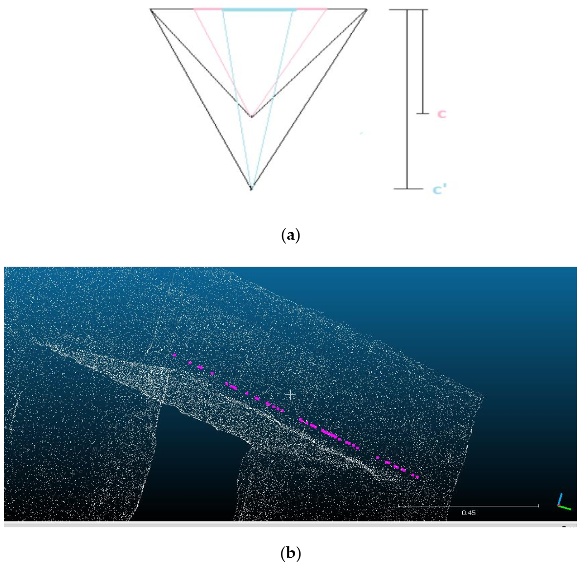
Finally, another problematic case is the depiction in the image of only one of the two sides of an edge (Figure 13a). Depending on the shooting angle this phenomenon may cause some problems for the algorithm. The rays from the camera “penetrate” the point cloud as shown schematically in Figure 13b and the algorithm fails. Depending on the angle of the camera axis, the points selected on the image are too close, but not exactly on the edge. The plane and the threshold used by the algorithm returns the two pink colored edges in Figure 13b, instead of the correct black one. This is attributed to the density of the point cloud and the fact that during scanning it is not certain that points exactly on the edge were registered by the scanner. The algorithm selects either of the two pink edges depending on whether the selected one is closest to the perspective center or back projected closer to the initially detected edge on the image. One suggestion for solving this problem is to limit the threshold or foresee a denser point cloud at the time of data acquisition.
7. Discussion and Concluding Remarks
In this paper, an effective automated method for detecting 3D straight edges in unorganized point clouds using the basic notions of Analytical Geometry and standard Photogrammetry is proposed. The implementation of the algorithm requires a point cloud and digital images with known exterior orientation, both in the same coordinate system. The edges are first detected on the images and the algorithm connects them to the 3D points of the point cloud that belong to each one of them.
The main characteristics of the proposed algorithm are:
- It exploits the geometric and spatial relationships of the oriented digital images and the available point cloud, thus directly connecting 2D image coordinates and 3D space coordinates.
- It can detect all the 3D edges for which the user has identified their depiction on the digital images, thus contributing to the automation of the production of two-dimensional vector drawings.
- It is a robust procedure, as it has been evaluated under different cases with varying image scale, image rotations, edge inclination, and length, thus distinguishing spatially adjacent, collinear, coaxial lines in complex neighborhoods.
In terms of execution time, all experiments were performed on an Intel i7-6500U CPU (2.50 GHz) system with 8 GB RAM. The time needed to perform the algorithm execution for the point cloud of the Temple of Demeter (750,000 points) was 25–30 s. This starts at the introduction of the image edge points and includes the transformation of the point cloud to a matrix form for Python to access it properly and the various inputs by the user (Figure 2). The clock stops when the edges are presented in CloudCompare. It is obvious that the execution time greatly depends on the complexity of the object and the size of the point cloud. Moreover, the existence of more edges parallel to the sought one in the point cloud is likely to slow down the process. It is estimated that for a point cloud with, e.g., 7 million points, the process will need about 90 s.
The experimental results show that the proposed algorithm is successful and meets the expectations of automation set at the beginning. Straight 3D edges are detected using the unique perception of defining the different planes using the edges depicted on images and their perspective centers and exterior orientation parameters to describe 3D space. The results have shown that the required accuracy is achieved, and that the method provides robust solutions in a short amount of computing time. In comparison with state-of-the-art methods, the proposed algorithm can obtain satisfactory results both qualitatively and quantitatively. Moreover, the uncertainties of the results of our proposed method were analyzed by confronting difficulties the algorithm may face during its operation.
The conclusions focus on the accuracy with which the edges are detected and on whether the user can influence it. The evaluation of the algorithm is based on several parameters, validating its success.
The first characteristic that determines the quality of the edges detected and which cannot be changed is the inherent accuracy and density of the point cloud. This depends on the equipment used for the acquisition and the parameters applied in the field. In addition, the object itself, especially in the case of cultural heritage buildings, may present deformations due to loss of material (e.g., weathering, intense use destructions, etc.), leading to practically non-existent edges, or edges that are not well defined. These cases should be examined and identified before the implementation of the algorithm.
The implementation parameters of the RANSAC algorithm also affect the accuracy with which 3D edges are detected. Of course, the user can intervene in this to improve the results. The actions that need to be done are, firstly, to correctly interpret the surfaces and their peculiarities. Secondly, through the default value, i.e., the threshold, to capture the correct interpretation of the properties of the surfaces in the results. That is, to correctly locate the inlier points from which the optimal mathematical model of the planes will be calculated.
In cases where there is a deviation presented to the user by the algorithm (Figure 2), several adjustments should be performed to locate the optimal edge and check how the results are differentiated. These adjustments include (i) the input of the correct accuracy of the pixel coordinates used as input data, (ii) the length of the input edge, and (iii) the use of at least the calibrated value of the camera constant for each image if it is known. Finally, in images with strong perspective distortions, it is obviously important to prefer the detection of edges using their full length and not a small part of them. Hence, it is important to detect the desired edge, if possible, in an image where both of its sides are clearly visible (Figure 14). These limitations ensure the smooth operation of the algorithm and lead to successful results.
The algorithm, as developed, experimentally implemented, and assessed, is promising. To this direction, some improvements are suggested to enhance its functionality and usefulness. Firstly, the detection of the 2D edges on the images should be automated, as the whole procedure is based on their fast and reliable determination. There are many edge detection algorithms that may be improved and become part of the algorithm proposed [28,29,30,31,32]. Secondly, perspective distortions should be avoided, as they adversely affect the implementation of the algorithm. This should be kept in mind at the time of image acquisition.
Thirdly, an additional constraint could be included in the implementation of the RANSAC algorithm. In cases of the determination of two edges on either side of the desired one (Figure 14b), provided they are too close, i.e., less than a threshold set by the user, the sought edge could be determined as the intersection of the two planes of the dihedral angle. Furthermore, the algorithm is being tested in more and diverse datasets to prove its robustness and efficiency. A major improvement at the stage of finalization [33] is the automated vectorization of the extracted 3D edges. Research so far has shown that the vectorization, e.g., in “dxf” format, may be realized by implementing the RANSAC algorithm again. Finally, a major improvement planned is the introduction of the detection of non-planar mathematical surfaces, i.e., cylindrical, or conical shapes, thus extending the algorithm to the detection of non-straight 3D edges. In this way the automated production of vector drawings will be greatly enhanced.
Author Contributions
Conceptualization, Andreas Georgopoulos; Methodology, Andreas Georgopoulos; Software, Maria Melina Dolapsaki; Validation, Maria Melina Dolapsaki, Andreas Georgopoulos; Formal Analysis, Maria Melina Dolapsaki, Andreas Georgopoulos; Writing—Original Draft Preparation, Maria Melina Dolapsaki; Writing—Review & Editing, Andreas Georgopoulos; Supervision, Andreas Georgopoulos. All authors have read and agreed to the published version of the manuscript.
Funding
This research received no external funding.
Institutional Review Board Statement
Not applicable.
Informed Consent Statement
Not applicable.
Conflicts of Interest
The authors declare no conflict of interest.
References
- Naci, Y. Documentation of cultural heritage using digital photogrammetry and laser scanning. J. Cult. Herit. 2007, 8, 423–427. [Google Scholar] [CrossRef]
- Briese, C.; Pfeifer, N. Towards automatic feature line modelling from terrestrial laser scanner data. Int. Arch. Photogr. Remote Sens. Spat. Inf. Sci 2008, XXXVII Pt B5, 463–468. [Google Scholar]
- Canciani, M.; Falcolini, C.; Saccone, M.; Spadafora, G. From point clouds to architectural models: Algorithms for Shape reconstruction. In Proceedings of the International Archives of the Photogrammetry, Remote Sensing and Spatial Information Sciences, 20133D-ARCH 2013—3D Virtual Reconstruction and Visualization of Complex Architectures, Trento, Italy, 25–26 February 2013; Volume XL-5/W1. [Google Scholar]
- Kersten, T.; Büyüksalih, G.; Baz, I.; Jacobsen, K. Documentation of Istanbul historic peninsula by kinematic terrestrial laser scanning. Photogramm. Record 2009, 24, 122–138. [Google Scholar] [CrossRef]
- Tryfona, M.S.; Georgopoulos, A. 3D Image based geometric documentation of the tower of winds. Int. Arch. Phot. Remote Sens. Spatial Inf. Sci. 2016, 41, 969–975. [Google Scholar] [CrossRef]
- Förstner, W. Image analysis techniques for digital photogrammetry. In Proceedings of the 42nd Photogrammetrische Woche, Stuttgart, Germany, 11–16 September 1989; pp. 205–221. [Google Scholar]
- Ando, S. Image field categorization and edge/corner detection from gradient covariance. IEEE Trans. Pattern Anal. Mach. Intell. 2000, 2, 179–190. [Google Scholar] [CrossRef]
- Frei, W.; Chen, C.C. Fast boundary detection: A generalization and a new algorithm. IEEE Trans. Comput. 1977, 10, 988–998. [Google Scholar] [CrossRef]
- Briese, C.; Pfeifer, N. Line based reconstruction from terrestrial laser scanning data. J. Appl. Geod. 2008, 2, 85–95. [Google Scholar] [CrossRef]
- Bazazian, D.; Casas, J.R.; Ruiz-Hidalgo, J. Fast and robust edge extraction in unorganized point clouds. In Proceedings of the 2015 International Conference on Digital Image Computing: Techniques and Applications (DICTA), Adelaide, Australia, 23–25 November 2015; pp. 1–8. [Google Scholar] [CrossRef] [Green Version]
- Lin, Y.B.; Wang, C.; Cheng, J. Line segment extraction for large scale unorganized point clouds. ISPRS J. Phot. Remote Sens. 2015, 102, 172–183. [Google Scholar] [CrossRef]
- Cheng, L.; Chen, S.; Liu, X. Registration of laser scanning point clouds: A review. Sensors 2018, 18, 1641. [Google Scholar] [CrossRef] [Green Version]
- Fleischman, S.; Cohenor, D.; Silva, T. Robust moving least-squares fitting with sharp features. ACM Trans. Graph. 2005, 24, 544–552. [Google Scholar] [CrossRef]
- Daniels, J.; Ochotta, T.; Ha, L.K. Spline-based feature curves from point sampled geometry. Vis. Comput. 2008, 24, 449–462. [Google Scholar] [CrossRef] [Green Version]
- Oztireli, C.; Guennebaud, G.; Gross, M. Feature preserving point set surfaces based on non-linear kernel regression. Comput. Graph. Forum 2009, 28, 493–501. [Google Scholar] [CrossRef] [Green Version]
- Yang, M.Y.; Förstner, W. Plane Detection on Point Cloud, Technical Report Nr. 1; Department of Photogrammetry Institute of Geodesy and Geoinformation University of Bonn: Bonn, Germany, 2010. [Google Scholar]
- Ni, H.; Lin, X.; Ning, X.; Zhang, J. Edge Detection and Feature Line Tracing in 3D-Point Clouds by Analyzing Geometric Properties of Neighborhoods. Remote. Sens. 2016, 8, 710. [Google Scholar] [CrossRef] [Green Version]
- Gumhold, S.; Wang, X.; Macleod, R. Feature extraction from point clouds. In Proceedings of the 10th International Meshing Roundtable, Sandia National Laboratory, Newport Beach, CA, USA, 7–10 October 2001; pp. 293–305. [Google Scholar]
- Weber, C.; Hahmann, S.; Hagen, H. Sharp feature detection in point clouds. In Proceedings of the Shape modelling international conference, Aix-en-Provence, France, 21–23 June 2010; pp. 175–186. [Google Scholar]
- Weber, C.; Hahmann, S.; Hagen, H. Methods for feature detection in point clouds. In Proceedings of the Visualization of Large and Unstructured Data Sets-IRTG Workshop, Bodega Bay, CA, USA, 19–21 March 2010; pp. 90–99. [Google Scholar]
- Weber, C.; Hahmann, S.; Hagen, H.; Bonneau, G. Sharp feature preserving MLS surface reconstruction based on local feature line approximations. Graph. Models 2012, 74, 335345. [Google Scholar] [CrossRef] [Green Version]
- Mitropoulou, A.; Georgopoulos, A. An Automated Process to Detect Edges in Unorganized Point Clouds. ISPRS Ann. Photogramm. Remote. Sens. Spat. Inf. Sci. 2019, IV-2/W6, 99–105. [Google Scholar] [CrossRef] [Green Version]
- Ben-Shabat, Y.; Avraham, T.; Lindenbaum, M.; Fischer, A. Graph based over-segmentation methods for 3D point clouds. Comput. Vis. Image Underst. 2018, 174, 12–23. [Google Scholar] [CrossRef] [Green Version]
- Hackel, T.; Wegner, J.D.; Schindler, K. Contour detection in unstructured point clouds. In Proceedings of the IEEE Conference on Computer Vision and Pattern Recognition (CVPR), Las Vegas, NV, USA, 27 June 2016; pp. 1610–1618. [Google Scholar] [CrossRef]
- Grilli, E.; Menna, F.; Remondino, F. A review of point clouds segmentation and classification algorithms. In Proceedings of the International Archives of Photogrammetry, Remote Sensing and Spatial Information Sciences, 3D Arch, Nafplio, Greece, 1–3 March 2017; p. 339. [Google Scholar]
- Hu, Z.; Zhen, M.; Bai, X.; Fu, H.; Tai, C.L. Jsenet: Joint semantic segmentation and edge detection network for 3D point clouds. arXiv 2020, arXiv:2007.06888. [Google Scholar]
- Fischler, M.A.; Bolles, R.C. Random sample consensus: A paradigm for model fitting with applications to image analysis and automated cartography. Commun. ACM 1981, 24, 381–395. [Google Scholar] [CrossRef]
- Dhankhar, P.; Sahu, N. A review and research of edge detection techniques for image segmentation. Int. J. Comput. Sci. Mob. Comput. 2013, 2, 86–92. [Google Scholar]
- Mehta, A.; Lehri, H.; Thakur, P.; Tambe, S. Exploring Methods to Improve Edge Detection with Canny Algorithm. Bachelor’s Thesis, Department of Computer Science and Information Technology of Veermata Jijabai Technological Institute, Mumbai, India, 2014. [Google Scholar]
- Kumar, M.; Saxena, R. Algorithm and technique on various edge detection: A survey. Signal Image Process. Int. J. 2013, 4, 65. [Google Scholar] [CrossRef]
- Maini, R.; Aggarwal, H. Study and comparison of various image edge detection techniques. Int. J. Image Process. 2009, 3, 83–90. [Google Scholar]
- Shrivakshan, G.T.; Chandrasekar, C. A Comparison of various edge detection techniques used in image processing. IJCSI Int. J. Comput. Sci. Issues 2012, 9, 1694–1814. [Google Scholar]
- Betsas, T. Automated Detection of Edges in Point Clouds using Semantic Information. Bachelor’s Thesis, School of Rural & Surveying Engineering, National Technical University of Athens, Athens, Greece, 2021. Unpublished (In Greece). [Google Scholar] [CrossRef]
Figure 1.
The main idea of the proposed algorithm.

Figure 2.
The flowchart of the developed algorithm.

Figure 3.
The Temple of Demeter on Naxos (© the authors).

Figure 4.
Results of the implementation of the first part of the algorithm to the simulation data. In (a) the original 3D point cloud, in (b) the same point cloud as projected on the image and in (c) the resulting point cloud after the rigid body transformation. In (d) the 2D edge of the inserted image is shown, in (e) shows the transformed 3D edge in the 3D space and in (f) the transformed edge is displayed.


Figure 5.
Results of the implementation of the first part of the algorithm to the real-world data. (a) the point cloud with 750,000 points, (b) the selected 2D edge on one image, (c) the 2D line as represented in image space, (d) the 2D line transformed and related to global reference system and (e) the section of the determined plane with the point cloud.


Figure 6.
Candidate edges (#1–8) after the first part of the algorithm.

Figure 7.
Representation of the angular difference between the plane describing reality and the plane determined by the algorithm used.
Figure 7.
Representation of the angular difference between the plane describing reality and the plane determined by the algorithm used.

Figure 8.
Display of the selected 3D points belonging to the requested 3D edge using the algorithm, (colored in purple) compared to the real word 3D edge obtained by the 3D scanner (colored in green).
Figure 8.
Display of the selected 3D points belonging to the requested 3D edge using the algorithm, (colored in purple) compared to the real word 3D edge obtained by the 3D scanner (colored in green).

Figure 9.
Display of a histogram showing how successfully the two 3D edges projected in Figure 8 as adapted to each other (differences in m).
Figure 9.
Display of a histogram showing how successfully the two 3D edges projected in Figure 8 as adapted to each other (differences in m).

Figure 10.
(a) The effect on the bundle of using the wrong focal length; (b) erroneous localization of 3D edge due to using nominal focal length.
Figure 10.
(a) The effect on the bundle of using the wrong focal length; (b) erroneous localization of 3D edge due to using nominal focal length.

Figure 11.
Comparison of edge points detected using the calibrated focal length and the original 3D edge in the point cloud.
Figure 11.
Comparison of edge points detected using the calibrated focal length and the original 3D edge in the point cloud.

Figure 12.
Display of the results of the algorithm when used on an edge depicting (a) the whole edge resulting in the pink edge in (c); and (b) a small part of the edge resulting in the white edge on (c).
Figure 12.
Display of the results of the algorithm when used on an edge depicting (a) the whole edge resulting in the pink edge in (c); and (b) a small part of the edge resulting in the white edge on (c).

Figure 13.
Representation of the problematic scenario at the time of image acquisition using real data from the temple of Demeter (a) and the problem analyzed in a drawing (b).
Figure 13.
Representation of the problematic scenario at the time of image acquisition using real data from the temple of Demeter (a) and the problem analyzed in a drawing (b).

Figure 14.
Edges depicted frontally with both sides imaged (a) or just one side (b). Result of successful localization of edge (c) obtained using (b).
Figure 14.
Edges depicted frontally with both sides imaged (a) or just one side (b). Result of successful localization of edge (c) obtained using (b).

Publisher’s Note: MDPI stays neutral with regard to jurisdictional claims in published maps and institutional affiliations. |
© 2021 by the authors. Licensee MDPI, Basel, Switzerland. This article is an open access article distributed under the terms and conditions of the Creative Commons Attribution (CC BY) license (https://creativecommons.org/licenses/by/4.0/).
Share and Cite
MDPI and ACS Style
Dolapsaki, M.M.; Georgopoulos, A. Edge Detection in 3D Point Clouds Using Digital Images. ISPRS Int. J. Geo-Inf. 2021, 10, 229. https://0-doi-org.brum.beds.ac.uk/10.3390/ijgi10040229
AMA Style
Dolapsaki MM, Georgopoulos A. Edge Detection in 3D Point Clouds Using Digital Images. ISPRS International Journal of Geo-Information. 2021; 10(4):229. https://0-doi-org.brum.beds.ac.uk/10.3390/ijgi10040229
Chicago/Turabian StyleDolapsaki, Maria Melina, and Andreas Georgopoulos. 2021. "Edge Detection in 3D Point Clouds Using Digital Images" ISPRS International Journal of Geo-Information 10, no. 4: 229. https://0-doi-org.brum.beds.ac.uk/10.3390/ijgi10040229
Note that from the first issue of 2016, this journal uses article numbers instead of page numbers. See further details here.