1. Introduction
In recent years, travel methods based on the shared use of micro-mobility electric vehicles have emerged in most cities, offering an alternative to traditional transportation systems [
1,
2,
3]. The popularity of shared micro-mobility services has spread widely. They are used in trips to urban centers or as an alternative for the first and last mile of metropolitan journeys [
4]. These mobility systems include shared use of bicycles, motorcycles and scooters, or other low-velocity modes, in docked or dockless service systems. In either case, but particularly in dockless services, the system is based on an intensive use of geolocation through smartphones: apps that allow users to locate and unblock vehicles and leave them anywhere when the journey has ended [
3,
5,
6,
7].
One of the most common forms of micro-mobility is the moped-style scooter, on which we will focus this research. Since it first appeared in the 2010s, its use has continued to grow at an increasing pace every year. Although the Coronavirus disease 2019 (COVID-19) pandemic is restructuring the sector and affecting many companies and cities, currently, there are nearly 80 operators worldwide, with around 9 million registered users in over 120 cities [
8]. The rapid growth of these micro-mobility systems has major implications for political and urban planning decisions related to mobility and the choice of transportation [
9].
Shared micro-mobility services offer benefits for the city and its users [
10]. In most cases, they are electric bicycles or vehicles, thus favoring environmentally-friendly forms of mobility, in which flexibility avoids the traffic congestion that characterizes many urban centers in the metropolitan areas where they operate. Thus, these systems help to reduce the use of cars, which, in turn, cuts greenhouse gas emissions and has benefits for the health of users and the population, in general. But they also improve mobility in urban centers, thus contributing to economic development [
11]. However, together with the above benefits, the process of increased integration of dockless shared mobility vehicles is also leading to problems, which are in turn creating major tension in urban governance [
12,
13]. These problems have to do, for example, with excess supply, the bad behavior of users, the unauthorized use of public spaces for riding the vehicles, and, above all, inadequate parking.
In fact, one of the biggest sources of conflict in the new forms of shared mobility in cities is vehicle parking. Often, scooters, bicycles, and even motorcycles appear on sidewalks, badly parked, or simply left on the ground, occupying a space designed for pedestrians. On sidewalks, where the space for pedestrians is limited, the inconvenience is even greater. It also affects particularly vulnerable groups, such as people with reduced mobility [
14]. A number of measures are already being taken, for example, through incentives to the users themselves [
15], but others have to be implemented to regulate the zones for parking. One low-cost solution is to reserve certain spaces for these shared mobility vehicles. Such parking spaces may simply be some of the spaces that today are used for private vehicles. In this paper, the use of Geographic information system (GIS) location-allocation models has been tested to find the best location for these parking spaces or shared vehicles docks.
We have been able to use data generated by the shared mobility systems themselves for our location-allocation models, allowing us to locate the demand for vehicles with a high level of spatial and temporal details. The apps used to manage these systems store the Global Positioning System (GPS) data on the origin and destination of the journey. These data provide information on the locations where there is demand for the system based on the trips actually made.
The aim of this research is to find parking spaces for shared motorcycle services based on GIS location-assignation models and considering the varying distribution of demand throughout the day. The center of Madrid and the GPS data of the company Muving (one of the city’s main operators) have been used for the case study. As well as searching for the location of parking spaces for motorbikes, our interest has been to carry out an analysis of how variations in the distribution of demand over the course of the day affects the demand assigned to parking spaces. To do so, we have used the data of the date and time when the trip was made, and the coordinates of origin and destination captured by the GPS devices in the electric motorcycles themselves. These data have been segmented into three-time bands: morning (07:00–13:59), afternoon (14:00–18:59), and night (19:00–00:00). The results of this work allow us to detect the best locations for electric motorcycle parking spaces, depending on the time distribution of demand over the course of the whole day. This information is of interest to the shared mobility company, and also the local government. They will have spaces reserved where motorcycles can be parked, thus providing a partial response to the problems and conflicts generated by their parking.
The document is organized as follows:
Section 2 presents a review of the literature.
Section 3 presents the case study, while a description of the data, their processing, and the methodology used are presented in
Section 4. The results are presented in
Section 5, followed by the conclusions of the paper.
2. Literature Review
The research into micro-mobility services in cities has become an important topic in the international literature on urban mobility. Recent publications have analyzed the spatial and temporal patterns of vehicle use. These works have used the GPS records generated by the systems themselves, which store the history of the origins and destinations of the trips made by users. The data collected from the GPS systems installed in the shared mobility vehicles have been used to analyze the accessibility offered by these new systems [
16], spatiotemporal patterns of use [
17,
18,
19], and models for predicating demand and customer segmentation [
20].
A number of studies have used the GPS data from shared mobility vehicles to analyze the patterns of spatial distribution of trips made in these micro-mobility systems, focusing particularly in the case of the scooter-share and dockless bike-share systems, comparing how the different types of vehicle are used, or how they compete with some of the traditional means of transportation. This is the case of the work of McKenzie [
18], who analyzes the spatiotemporal use of scooters and bicycles, using the GPS data of the company Lime to compare the patterns of use of Lime vehicles with the system of public bicycles in Washington, DC. In a later work, McKenzie [
19] extends the analysis to all the micro-mobility companies and assesses the competition between micro-mobility and cars in terms of duration of trips within the city. Reck et al. [
21] also model the competition between different forms of micro-mobility. Other works have used patterns of mobility to identify differences between users, such as the mobility of habitual and occasional users [
20,
22], or to relate the types of trips with the conditions of the constructed space [
14,
23,
24].
The data on the spatial patters in the use of micro-mobility services have also been used to find solutions to the problems associated with parking vehicles. Hua et al. [
5] have estimated the demand for parking of three free-floating bike-sharing companies, using GPS data from the company Mobike and spatial cluster techniques to estimate the demand for parking and establish locations for parking spaces. These spatial clustering techniques have been used to find parking zones for free-floating bike-sharing systems using a multiscale geographic view [
25] or including a real-time approach [
14]. However, these works have focused mostly on free-floating bike-sharing services.
Some works have also used GIS location-allocation models for free-floating bike-sharing systems, following the methodology used previously for bike-sharing parking stations [
26], but using new data collected from GPS.
Zhang et al. [
7] propose a methodology for locating electrical walls or virtual geo-fences where bicycles can be parked without fixed stations. Their research uses GPS data on trips, collected by the company Mobike, and the maximizing coverage solution. Park and Young [
27] have created a model to determine location allocation using GPS taxi trajectory data to determine the best location for stations. Yang et al. [
28] formulated a methodology of space-time demand cubes to capture the demand for bicycles. They used GPS data from the bicycle system to study the distribution of demand and applied solutions for minimizing impedance and maximizing coverage with genetic algorithms. Other works suggest locating new stations using the solution of maximizing market share by including variables of proximity to restaurants, pubs, attractions and the coordinates of trips by users of the shared-bicycle system in the city of Baltimore, MD, USA [
1].
Less work has been done to look at moped-style scooter sharing, and there is very little that estimates optimal locations of some type of service for them, whether battery charging points or parking spaces. Among those that have appeared, some again use spatial clustering methods, such as Hua et al. [
5], who estimate the demand for parking of some companies in Nanjing (China) based on GPS data for the origins and destinations of the company Muving’s e-motorcycle trips. Chen et al. [
29] apply minimizing impedance and maximizing coverage solutions to locate recharging stations for the batteries used by e-scooters. However, none of them has made use of the time information in the data to consider the dynamic component of the use of the system in optimal location models.
4. Material and Methods
GIS location-allocation models work according to the distribution of demand for the service to be provided (in this case, the users of the mobility service), a distribution of candidate locations for the service, and a network to simulate movement from the location of the demand to the possible points (in this case, the street map of the central districts of the city of Madrid). This information is incorporated into the GIS in a vector format, through layers of points, where there is demand and candidate locations and lines for the network.
A number of different solutions are available based on this information to find the best locations and assign the demand to them. In general, solutions can be differentiated between those that put a premium on efficiency in accessing demand (covering the largest number of locations with a specific number of locations and at a given distance) and those geared to equity (covering the demand for the service by minimizing the distance to the demand as a whole). One of the most common solutions is known as p-median [
31], which is geared to equity. Its objective is to minimize the distances weighted by total demand to the locations of the service. In the case of the models that put a premium on efficiency, the solutions are based on maximizing the coverage of the demand for the service within a specific distance. Edmonds [
32] and, subsequently, Church and ReVelle [
33] formulated the problem of the location with maximum coverage, where a number of installations must be located to maximize the demand served within the stipulated standard of distance. Toregas et al. [
34] created a location model that finds a minimum number of locations to guarantee a standard service cover. In this paper, the solution that maximizes the demand covered within a certain threshold of distance has been used. The models were calculated using the Network Analyst extension in ArcGIS Desktop 10.6 (Redlands, CA, USA).
4.1. Data and Their Treatment for Creating the Model
The necessary information to implement the models and processes to prepare the data are presented in this section.
4.1.1. Street Network
This set of data was downloaded from the Open Street Map server with the help of QGIS software. The Network Analyst extension of ArcGIS Desktop 10.6 software was used to set up a network that simulates the movement of demand to the candidate sites.
4.1.2. Service Demand Data
The data used have been the information on system use itself. Thus, the origin and destination points of the trips from the e-motorcycles of the company Muving have been used. The records of trips were collected by the GPS devices in the motorcycles themselves. These records contain information on the use of the system from the months of February to December 2019, covering a total period of 11 months. Each trip includes the following information: customer identifier, vehicle identifier, duration, distance traveled, departure time, arrival time, and the coordinates of the origin and destination. In total the initial database amounted to 242,027 trips within the area covered by the study.
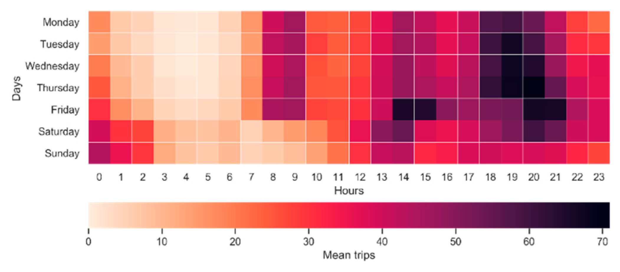
Figure 2 shows the average trips per hour and day. Every day the highest average trip was between 18:00 and 21:00 h. The origin of the trips was used as demand data for implementing the models.
4.1.3. Demand Data Cleaning
The set of initial data (242,027 trips) has been cleaned to eliminate atypical data (4995), leaving us finally with 237,062 trips. A box-plot was constructed to fine-tune the data cleaning by detecting atypical records according to the time and speed data of trips made, eliminating the data that were outside the upper and lower extreme of the graph. This eliminated trips with distances above those expected given the autonomy of the motorcycles (According to the characteristics of Muving’s motorcycles, trips greater than 70 km have been considered as measurement errors.). In addition, trips lasting less than 60 s (usually trips where the user has detected some problem and, finally, decided to not made the trip) and records where the duration of the trip did not match the distance traveled (e.g., long-distance trips made in very short periods of time) have been eliminated.
4.1.4. Data Aggregation
Once the data were debugged, they were aggregated spatially in a regular grid of cells measuring 50*50 m. This cells’ resolution has been established considering the size of the study area. This resolution allows an adequate level of detail for the proposed analysis without compromising the processing times in calculating the models in the GIS. The definition of the location of demand in the models took the centroid of each of the cells and the total trips with their origin there. The trips were also grouped together by time into three bands: morning (07:00–13:59), afternoon (14:00–18:59), and night (19:00–00:00).
4.2. Definition of the Candidate Locations for Parking Spaces
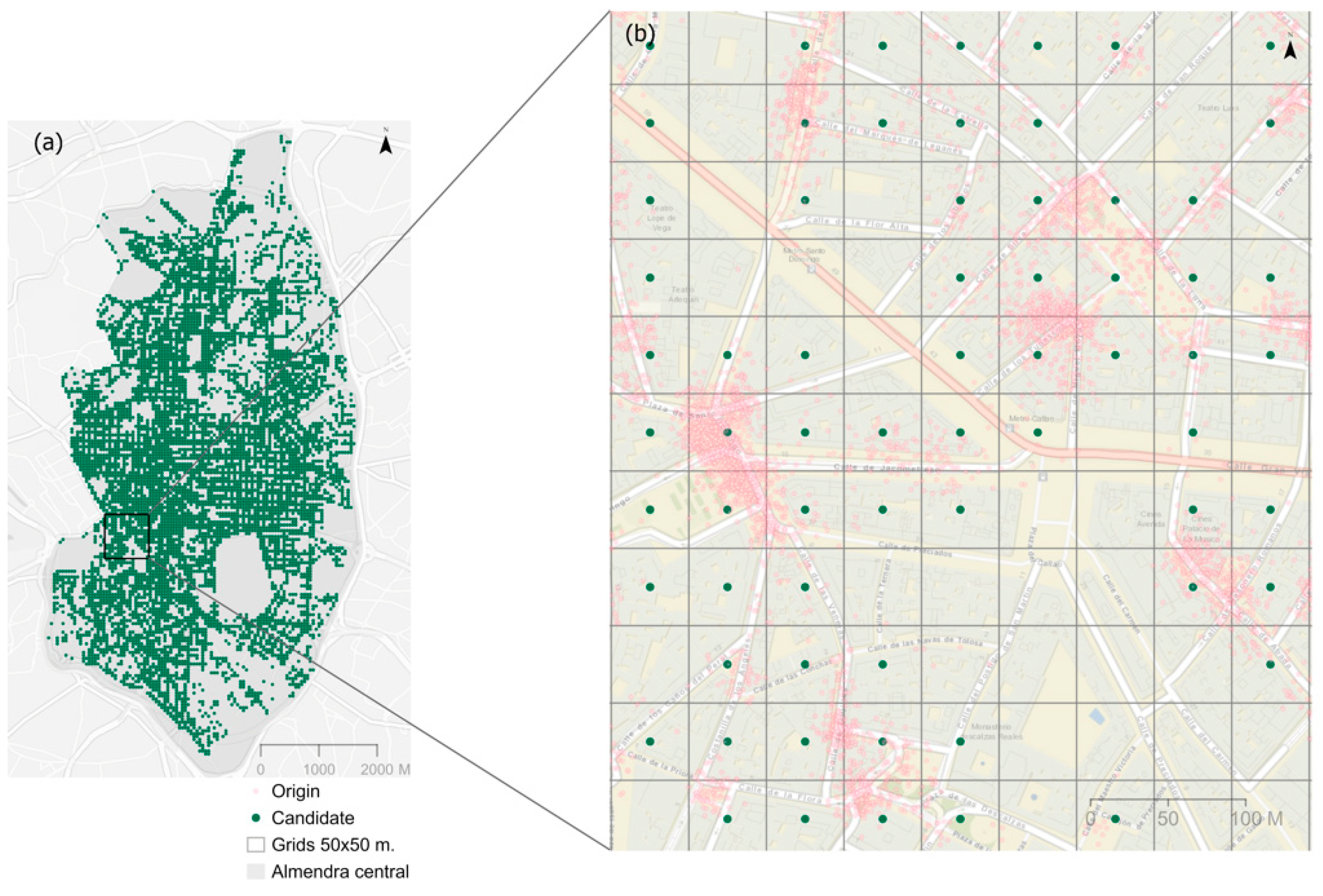
The candidate locations for the parking spaces were those cells that totaled more than five starting points for trips. With this selection, the number of candidates in the implementation of the location models is reduced, eliminating cells with very low demand. In total, there were 7735 candidate locations (
Figure 3a), covering the area of the study with a high spatial level.
Figure 3b shows how, with this selection, most of the demand is covered, and regularly distributed candidates are obtained.
4.3. Location-Allocation Model Definitions
The number of parking spaces to be located was initially estimated at 200, taking into account that the average fleet of motorcycles of the companies operating in the city is around 800 vehicles. Thus, the average capacity of these locations would be 4 vehicles. Similar scenarios with the same number of stations have been considered in bike-sharing programs for the same area [
26].
In addition, four-time scenarios were considered. The reference scenario took into account the distribution of total demand over the day, thus considering the demand of each cell as the sum of all the origins produced in it. This scenario was compared with three partial time scenarios (that considered the distribution of demand in each of the three-time bands into which the data were divided: morning (07:00–13:59), afternoon (14:00–18:59), and night (19:00–00:00).
The rest of the parameters of the model refer to the type of solution and the distance traveled by the user. With respect to the type of solution, the maximum coverage solution was used, taking as the maximum distance that a user would be prepared to walk to the motorcycle to be 200 m. This type of model offers locations that guarantee the maximum number of users are within this threshold of defined distance or cost of movement (200 m), always assigning the demand to the closest center [
33]. This solution and this distance have been used in previous studies on the optimal location of public bicycle stations in the city of Madrid itself [
26].
The equation used is as follows [
33]:
where
Ni is the set of candidate sites to provide coverage to the points of demand
i. A demand location is considered covered when the closest installation to the location of the demand is at a distance that is less than or equal to S. A demand point is not covered when the closest installation to the demand location is more than S [
33].
The type (1) restrictions allow y
i to be equal to 1 only when one or more installations are established in sites in the whole of N
i. The number of installations allocated is restricted or equal to p (2) [
33].
Based on the results of these models for the optimal location of the three time bands of morning, afternoon, and night, a process was developed to obtain a fifth solution (optimized scenario) in which these locations are combined as follows:
The starting point is the parking spaces that appear in the three time bands, eliminating the parking space with the lowest captured demand if parking spaces appear at less than 200 m apart.
To these parking spaces are added those that are active in the two bands of afternoon and night, unless they are within 200 m of one of the locations included in point 1, and eliminating the space with least assigned demand if it is within 200 m of another active location at the time.
To these are added the parking spaces that appear in both the morning and night bands, unless they are within 200 m of one of the locations included in points 1 and 2, and eliminating the space with least assigned demand if it is within 200 m of another active space in those two time bands.
To these are added the parking spaces that appear in both the morning and afternoon bands, unless they are within 200 m of one of the spaces included in the three points above and eliminating the space with least allocated demand if it is within 200 m of another active one at in those two time bands.
To these are added the parking spaces that appear in the night time band, unless they are within 200 m of one of the spaces included in the above points, and eliminating the space with less demand allocated if it is within 200 m of another active one in the night band.
To these are added the parking spaces that appear in the afternoon band, unless they are within 200 m of one of the spaces included in the above points, and eliminating that with least allocated demand if it is within 200 m of another active one in the afternoon band.
To these are added the parking spaces that appear in the morning band, unless they are within 200 m of one of the spaces included in the above points, and eliminating that with least demand allocated if it is within 200 m of another active one in the morning band.
This process has been automated using the model builder tool from the ArcGIS Pro software.
In summary, this paper considers five scenarios: (1) Reference scenario: using the distribution of the total demand over the day; (2) Partial scenario in the morning; (3) Partial scenario in the afternoon; (4) Partial scenario at night; (5) Optimized scenario: combined the solutions in the partial scenarios.
Finally, an indicator was calculated to discover the importance of each of the parking spaces selected in each time band (morning, afternoon, and night), comparing the level of demand allocated to each parking space in this time band as a proportion of the total demand in this time band with the demand allocated for the total demand as a proportion of the total demand, in accordance with the following equation:
where:
is the index of specialization at the parking space i in the time band m,
is the demand allocated to station i in the time band m,
is the total demand in the time band m,
is the demand allocated to station i in the reference situation with total demand, and
is total demand.
5. Results
This section presents the results of the research. First, the distribution of demand is show, both for the total of the day (reference scenario), and for the morning, afternoon, and night situations (partial scenarios). Then, the results for the reference scenario and the impacts of changes in demand throughout the day in that reference scenario are shown. The results of the partial scenarios and the optimized scenario are presented later. All of them are compared with the reference scenario
5.1. Distribution of Demand: Origin and Destination of Trips
The models are based on the distribution of the demand for trips, which will be considered as the distribution of demand.
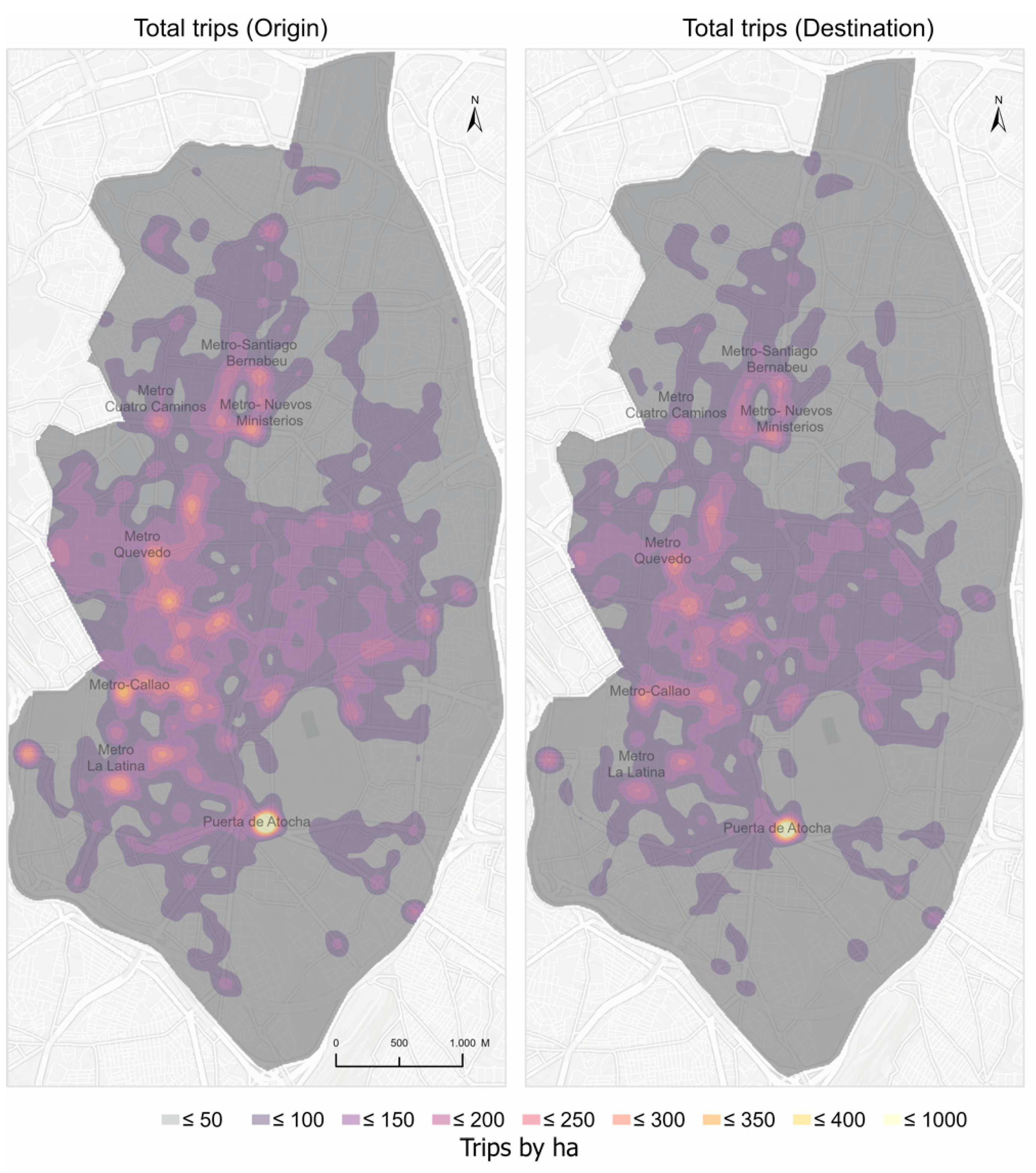
Figure 4 presents the density of trips per hectare, by origin and destination. A concentration can be seen in both origins and destinations in the central area and the Nuevos Ministerios axis. There is a great concentration of trips close to Puerta de Atocha station. The descriptive statistics of trips by origin and destination per hectare (
Table 1) give an average of 46.8 and 56.1 of trips per hectare, respectively, with relatively similar distributions, as shown by the coefficients of variation. The main difference lies in the greater concentration of trips with origin in the surroundings of train and metro stations, particularly in Atocha station, where there are a maximum of 687 origins of trips per hectare, and 564 destinations.
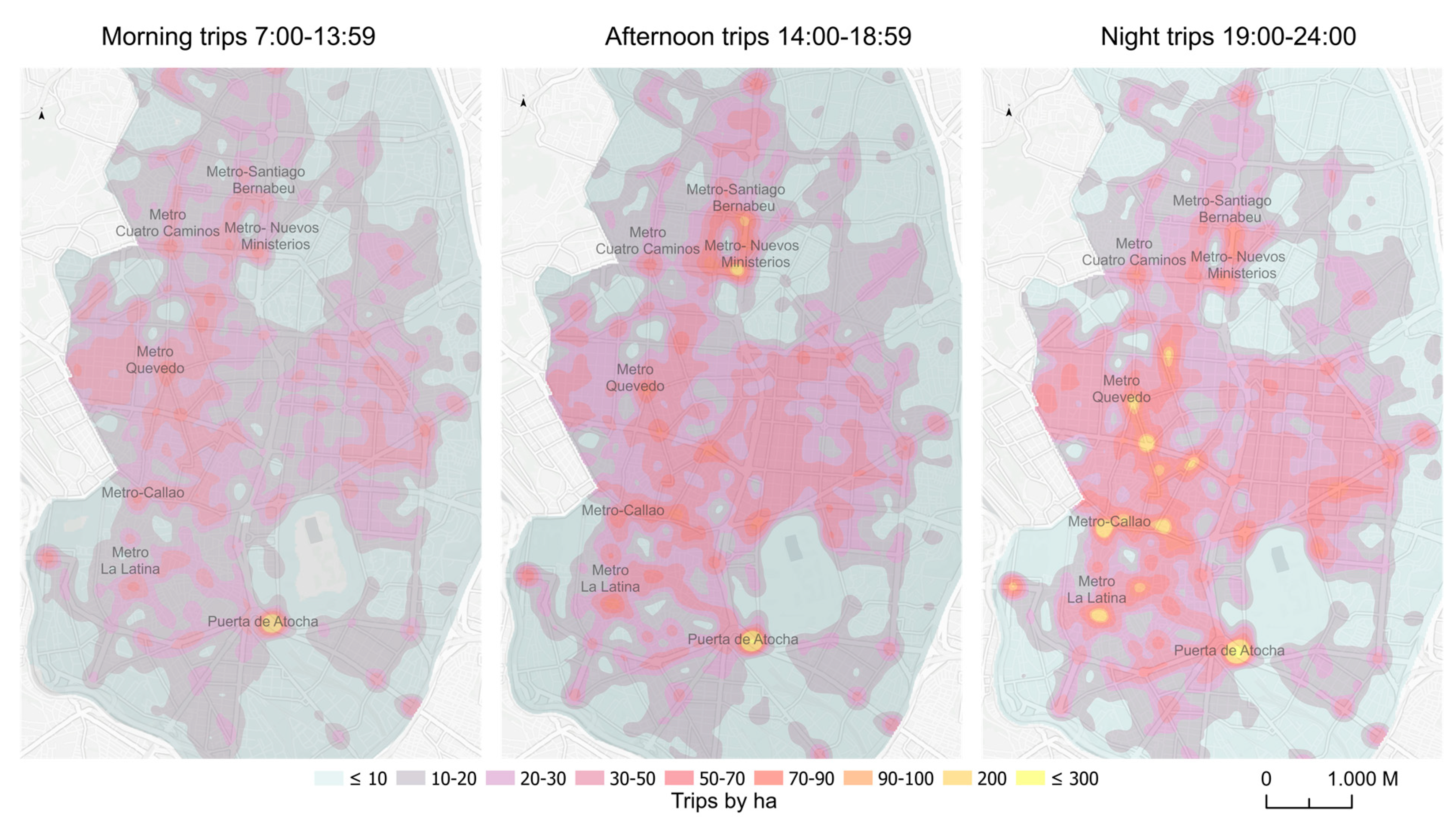
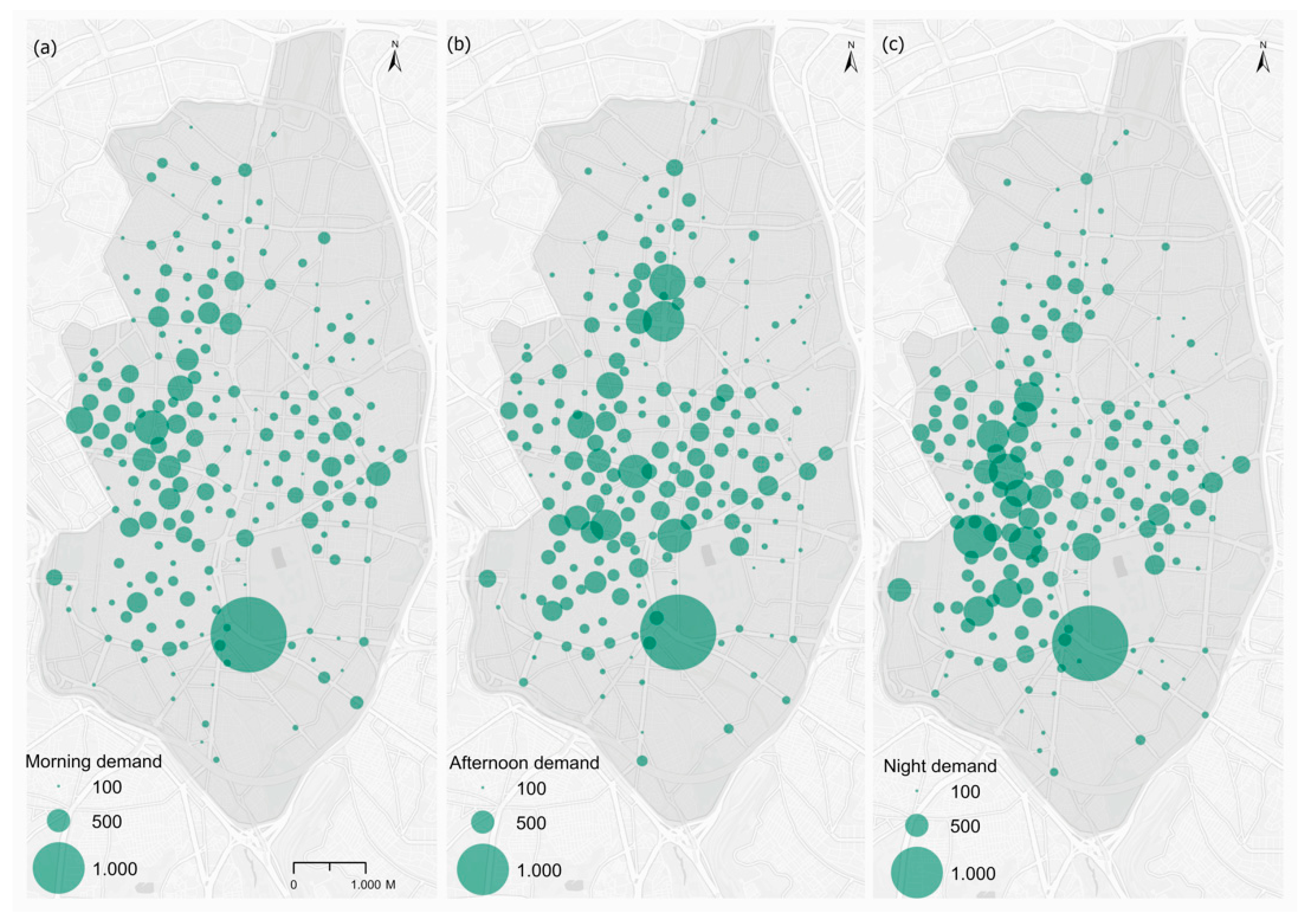
Figure 5 shows the distribution of demand grouped into the three-time bands under consideration. The system is used most at night, with average densities above 19 origins per hectare and values of over 200 origins per hectare in many zones in the center of the city (
Table 2). In contrast, the use of the system is much lower in the morning band, despite the band being 2 h longer. The afternoon presents an intermediary situation between the above two. As well as differences in the number of trips, there are also differences in their spatial concentration. In the morning, the spatial distribution is more homogenous, and the more residential zones have intensities similar to the zones with economic activities, as shown in the maps and lower coefficients of variation in this time band (
Table 2). In the afternoon, the greatest densities are concentrated in areas of economic activity, such as the office zone of Azca. At night, in turn, the distribution is more unequal, with densities of origins of trips being very high in leisure and restaurant areas of the Centro district.
5.2. Proposed Optimal Location of Parking Places for the Distribution of Total Demand
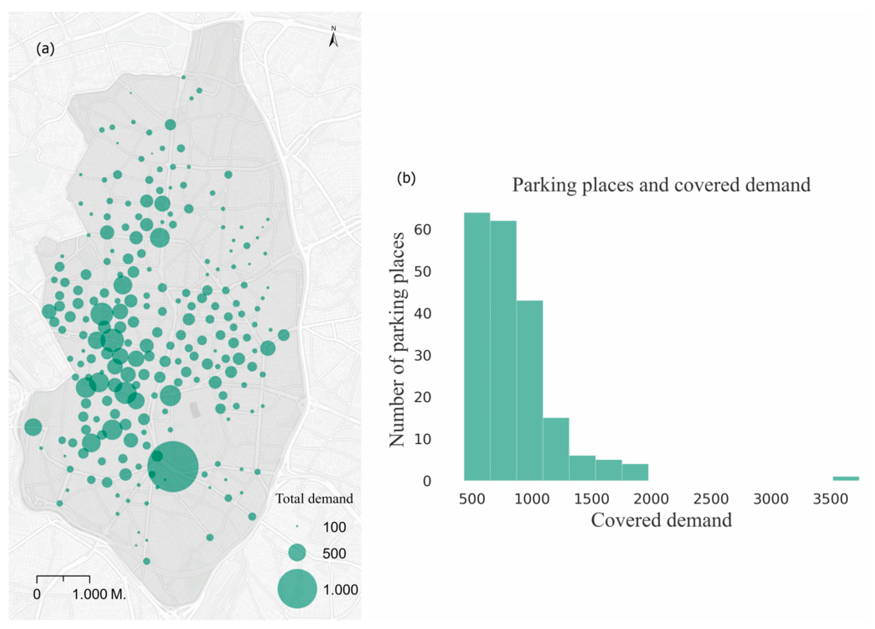
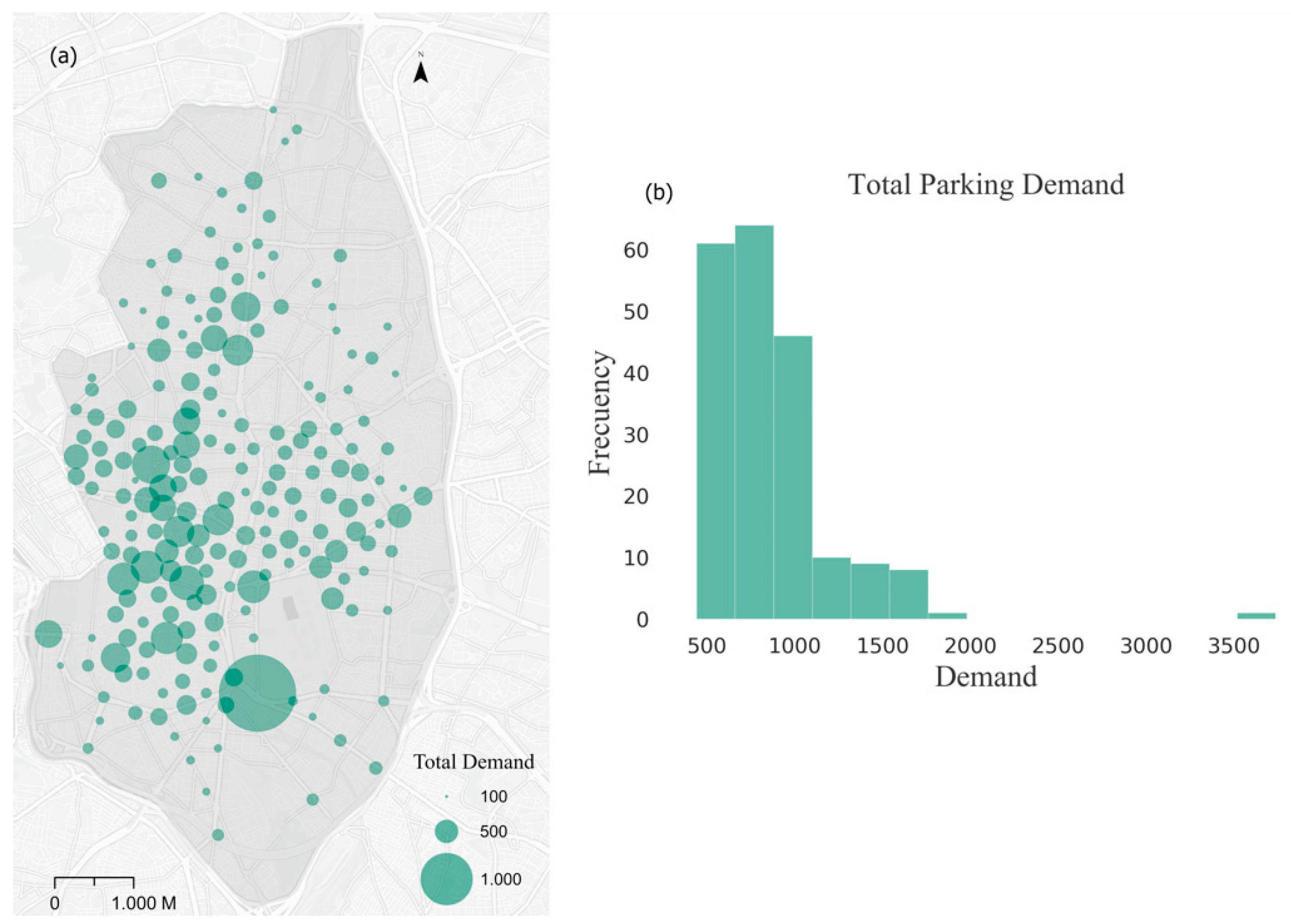
Figure 6 contains the results obtained taking into consideration the total daily trips by origin (reference scenario). The size of the symbol shows the total demand allocated to each of the parking spaces. With this distribution of 200 parking spaces, just over 170,000 of the origins of trips would be covered at a distance of 200 m, amounting to 72% of the total (
Table 3).
The greatest number of parking spaces is located in the zones of the Centro district, related to shopping, leisure and employment areas, as well as train stations and transportation interchanges (like Atocha and Nuevos Ministerios). The average of demand allocated per parking space is 850 trips, but the frequency timeline for parking spaces by demand allocated shows an asymmetrical distribution biased to the right, in which most of the parking spaces have allocated demand of less than 1000 trips for this period of 11 months (some 90 trips per month). Only around 30 parking spaces exceed the 1000 origins allocated, and, only in one case, in the area around Atocha station, there were over 2000 origins, with a total of 3300 (300 origins of trips per month).
5.3. Impact of the Changes in the Distribution of Demand during the Day
To discover the effects of the changing spatial distribution of demand during the day in the coverage of the proposed locations obtained in the reference scenario, below, the demand covered by these parking spaces in each of the three-time bands is calculated.
Table 4 shows how the percentage of coverage ranges between 69.1% of demand covered in the morning and 73.3% at night. The greater demand at night and its greater concentration in the central areas means that the efficiency of the network of parking spaces is greater in this time band than during the day as a whole, capturing 1.2% more demand at this time than in the situation with total demand. In contract, the greater dispersal of trips in the morning has an impact on the efficiency of the parking spaces in this time band, which capture 2.8% fewer origins of trips in this band.
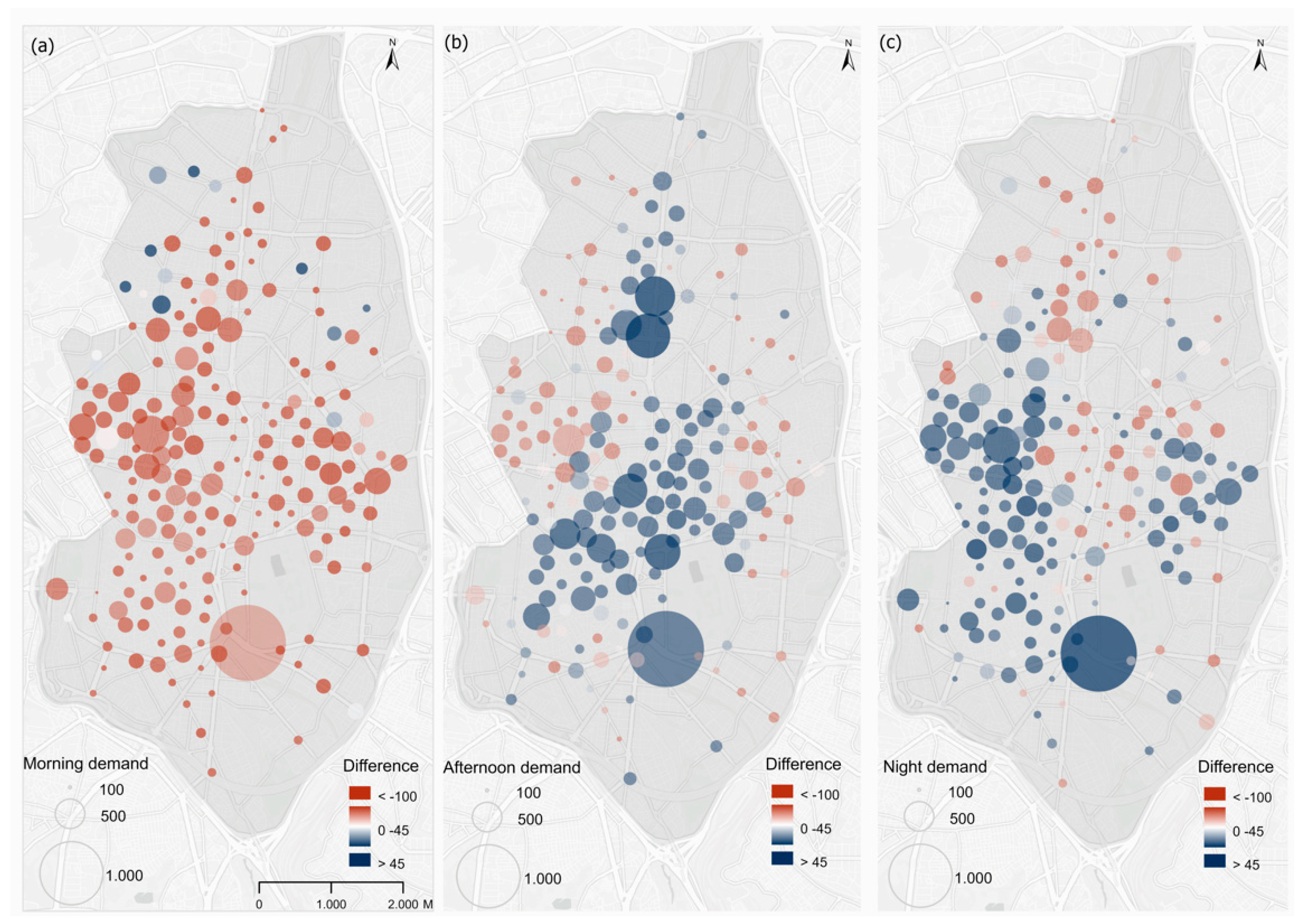
Figure 7 shows the demands allocated to each parking space according to time band (size of the symbols) and the differences between the demand allocated to each of the locations of the parking spaces between the time bands. The demand allocated to the parking spaces in the morning is much more homogenous than in the afternoon and at night, so although the most central parking spaces have greater allocated demand, the differences with respect to the more peripheral parking spaces are reduced and the only outstanding location is the parking space around Atocha station (in all three time bands). In contrast, in the afternoon the demand for parking spaces in the central areas and the areas of activity, particularly the Prado-Recoletos-Castellana axis, increases strongly, while the demand allocated to the parking spaces in the more peripheral residential areas is reduced. At night, these parking spaces in the Prado-Recoletos-Castellana axis once more lose allocated demand, while it is increased in the shopping and leisure areas of districts, such as Centro, Chamberí, and Salamanca.
Thus, if we look at the differences between time bands, the greater demand at night means that most of the parking spaces have more trips assigned at night than in the morning, although, in some residential zones in Tetuán and Salamanca, there are some parking spaces with more trips in the morning. These differences also appear between the morning and the afternoon, where the more residential zones have more trips in the morning and those with business activity capture more in the afternoon. There is a difference between the afternoon and night in the areas of activity around the Castellana, with a greater demand in the afternoon, and the shopping and leisure zones of districts, such as Chamberí and Centro, which are notable for the demand captured at night.
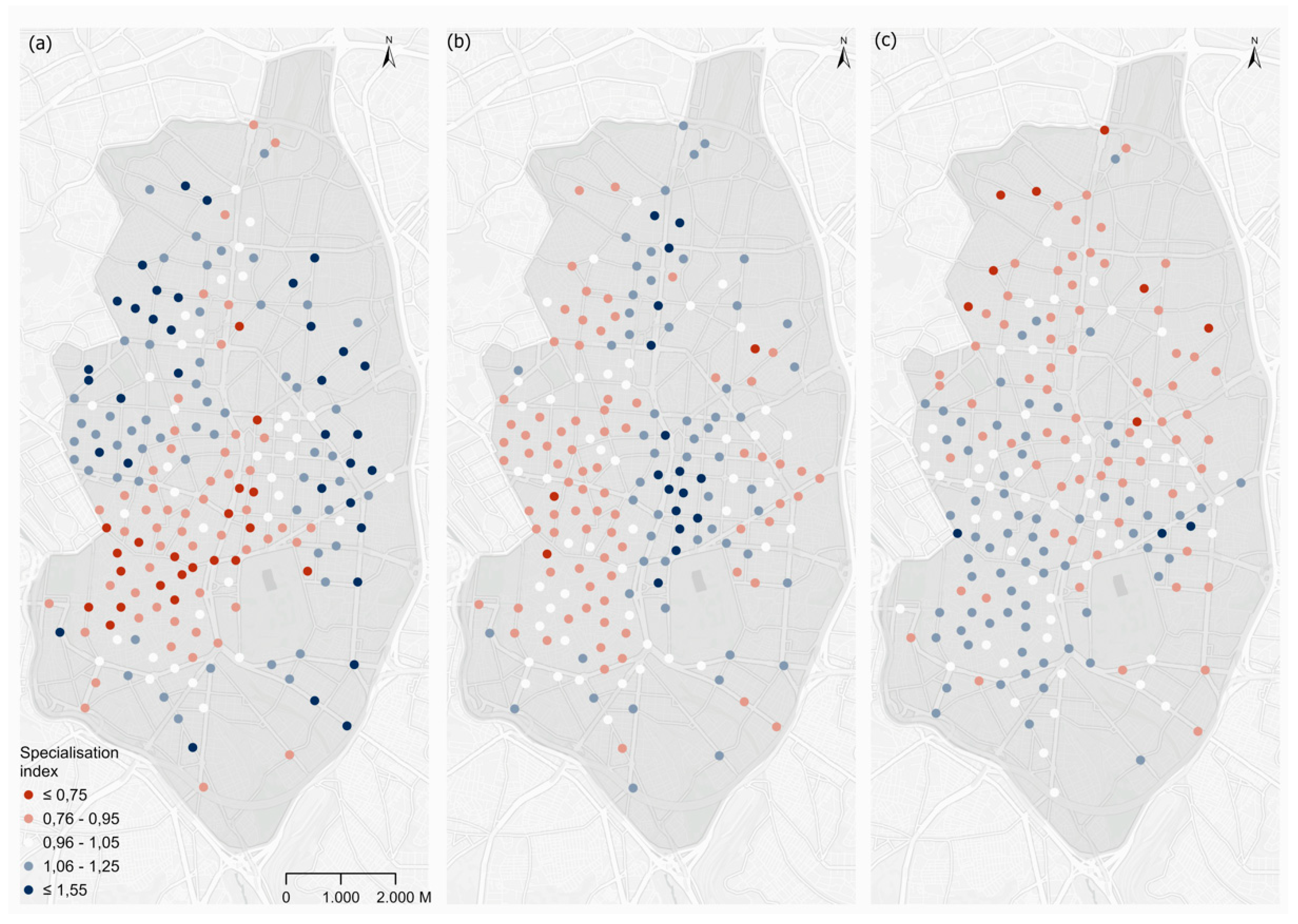
We have calculated indices of specialization to analyze the degree of importance of the demand captured in each parking space and in each time band, with respect to that captured in the reference scenario (with total demand). Here, the blue colors show parking spaces with a greater weight at a particular time, and the red parking spaces a lower weight with respect to the situation in the reference scenario (
Figure 8). The parking spaces which at this time have a behavior similar to the reference scenario are white. An optimal situation of the system would be where the parking spaces had similar allocated demand (circles of similar sizes in the above figure) and remained homogeneous over the course of the day (with the white colors being the main ones in the three time bands).
The results show very clearly the differences in the specialization of the stations according to the spaces with greater weight in residential areas in the morning (blue in the morning band), the office worker zones (blue in the afternoon), and leisure and restaurants (blue at night). The situation at night, when demand is greatest and, therefore, has the greatest influence in the reference scenario, has the lowest levels of specialization (values of around 1 and clear colors), while, in the morning, there are parking spaces that have a great deal of importance at that time (residential, with intense blue), or much less (areas of business activity, in red).
5.4. Models Adapted to the Changes in the Distribution of Demand
A calculation of models of location of the parking places for each of the time bands (partial scenarios) was attempted based on the distributions in the different time bands, to assess the improvements in the coverage of possible models that consider whether a parking space should be activated or not depending on the time. This solution would be something similar to parking places reserved for the delivery of goods or certain services, such as, for example, pharmacies, where parking is reserved for these activities within a particular time band. Nevertheless, it would have the limitation that some vehicles could remain in the parking space outside the time period allocated, which could increase costs if the company had to redistribute the vehicles.
Figure 9 shows the optimal locations of the parking spaces for each of the partial time scenarios and the total of origins of trips allocated to each of the parking spaces (in the size of the symbols). As can be seen, the distributions are relatively similar, although with a greater dispersion of parking spaces in the morning, where there are more in the residential areas bordering the area under study, and a more homogenous total distribution of allocated trips. In contrast, the distribution of parking spaces in the afternoon and above all at night is concentrated most strongly in the central areas, with the biggest differences between these parking spaces and those more peripheral in the total trips allocated. In any event, as can be seen in
Table 5, the increases in demand covered in the three cases compared with the reference scenario are very small. In the morning, the model captures 1% more of the origins of the trips in this time band than the reference scenario, while, in the afternoon and at night, the figure is barely 0.5% more.
Although the distributions are relatively similar, only 35 parking spaces appear active in the three time bands, just over 15% of the 200 located in each case (
Table 6). In contrast, more than 50% of those established in each time band do not appear in the other two periods. The greatest similarities are between the afternoon and night, which have 41 common parking spaces, while, between the morning and afternoon, there are 27, and, between morning and night, there are 26.
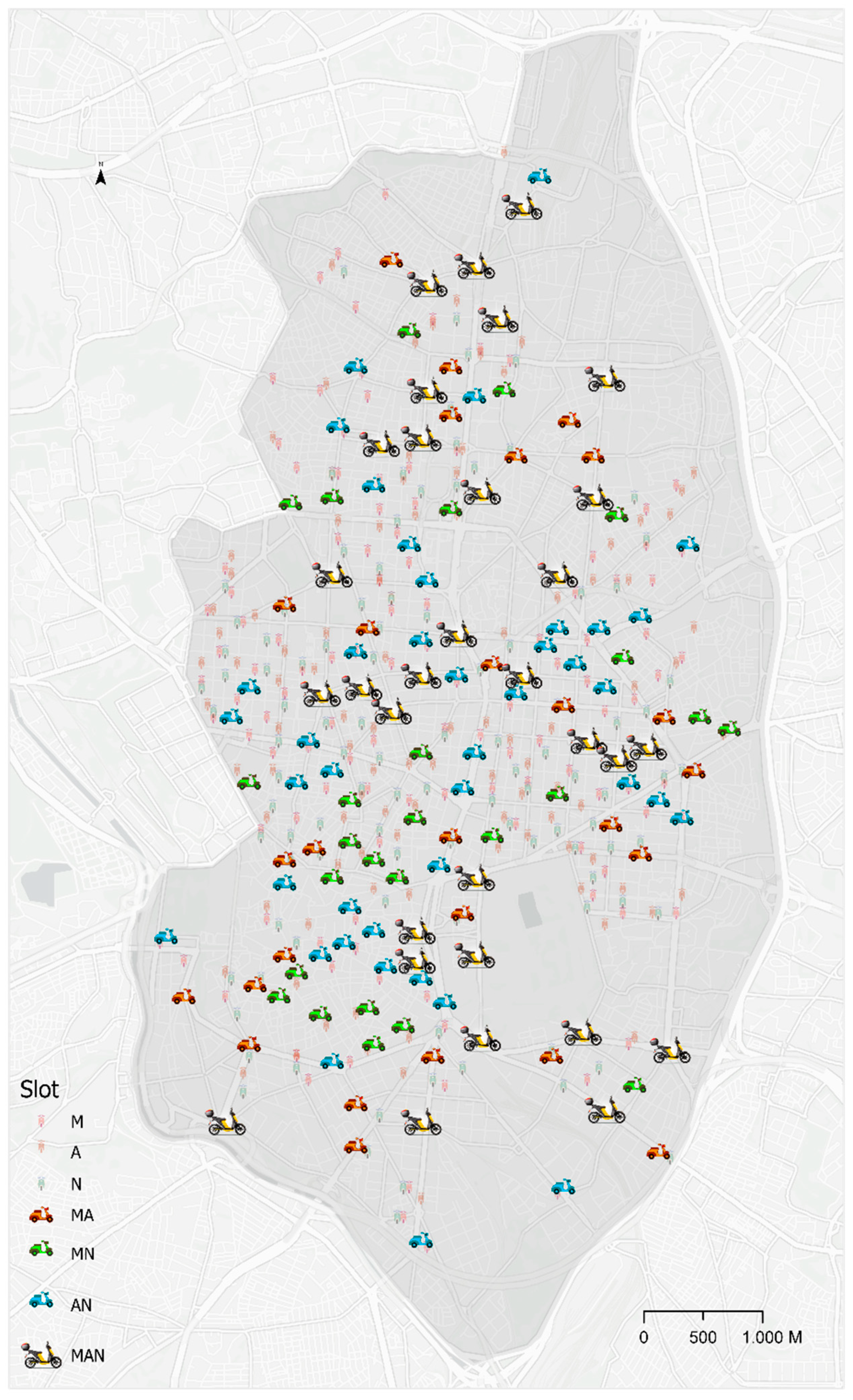
Figure 10 shows the spatial distribution of these parking spaces according to the time in which they appear.
On the basis of the above map, and following the methodology explained above, a last model for locating parking spaces has been obtained. This optimized scenario has a total of 229 parking spaces, which represents 14.5% more than in the initial reference scenario. With these parking spaces, the total number of origins covered is 178,982, or 75.5%, which represents 3.6% more than in the reference scenario with 200 parking spaces. This model not only has higher coverage in all the time bands but has the advantage of reducing the differences in the demand covered between the time bands (
Table 7 and
Figure 11).
6. Conclusions
In this study, GIS location-allocation models were used in order to find the best locations for parking micro-mobility system vehicles. Unlike previous works which have implemented the same methodology for free-floating bike sharing (e.g., References [
7,
27]), in this paper, we worked with a moped-style scooter and incorporated a dynamic perspective with respect to supply and demand. Our proposal used a set of data provided by the company Muving, which are collected from the GPS records of trips made by users.
The use of data from the system itself, taken as a variable of the location of demand within the models, allowed us to work with information of great spatio-temporal detail. Compared with previous works, in which demand is treated from a static perspective, here, we considered the distribution of demand in different time bands over the course of the day. Based on a model calculated using the distribution of total demand (reference scenario), we evaluated how the changes in the daily distribution of demand for trips influence the location of parking spaces. This dynamic perspective allowed us to evaluate the efficiency of the system and see how the variations in the distribution of demand affect the coverage of the service over the course of the day. In addition, it is possible to identify the importance of each parking space depending on the time of day, identifying those with most usage at a particular time and others that have a more continuous usage over the course of the day. Finally, we assessed the efficiency of a model adapted to these time variations in demand.
The results show that models of this type allow us to obtain an efficient distribution of parking spaces. With 200 parking spaces, 72% of the trips are within a distance of 200 m. This is an optimal solution, which would have a very low implementation cost, as they could be parking places currently allocated to cars. This efficiency is maintained over the course of the day, as, although the greater dispersion of trips in the morning band makes the coverage reduce slightly at this time, the decline is small, while during the night the demand is more concentrated, and the efficiency of the parking spaces increases. In addition, when we looked for optimal locations for parking spaces adapted to the changes in demand (partial scenarios), we found small gains in the demand covered, which barely allowed the coverage of 1% more of demand in the morning band and less than 1% in the afternoon and at night. Although there is no sudden reduction in the total coverage of the system between time bands, there does appear to be a marked specialization in parking spaces over time. The greater residential specialization in the periphery of the central area of Madrid means that the parking spaces in the periphery have a greater activity during the morning bands, while the spaces that are more central (commercial and leisure areas) are more active in the afternoon, and particularly at night. Finally, in the paper, we also proposed a solution that aims to adapt the locations of the parking spaces to the changing distribution in demand over the course of the day (optimized scenario). This is a simple solution, which combines the best locations in each of the time bands, looking for parking spaces that can maintain a high coverage and efficiency over the course of the day.
The methodology proposed here may be interesting to urban mobility planners and managers, who face the challenge of anticipating the impact of the new micro-mobility services in urban centers. Policies and actions must be designed that are capable of regulating the new demand for these systems, and particularly the problems and conflicts generated by the parking of the vehicles. It is also essential for the micro-mobility companies to implement joint actions with planners to allow a better service to be offered and to avoid conflicts with other forms of transport or with pedestrians, which generate a negative image of the system. In the search for these solutions, companies have the advantage of having very precise spatial and time information, as well as on the supply and demand for trips. These data can be used in a GIS to search for the best locations for parking spaces and to evaluate possible future scenarios.


