Article

High-Resolution Remote Sensing Image Segmentation Framework Based on Attention Mechanism and Adaptive Weighting

1
Department of Electrical Engineering & Information Technology, Shandong University of Science and Technology, Jinan 250031, China
2
Fujian Anta Logistics Information Technology Co. Ltd., Quanzhou 362200, China
3
Department of Finance and Economics, Shandong University of Science and Technology, Jinan 250031, China
*
Author to whom correspondence should be addressed.
ISPRS Int. J. Geo-Inf. 2021, 10(4), 241; https://0-doi-org.brum.beds.ac.uk/10.3390/ijgi10040241
Submission received: 11 February 2021 / Revised: 25 March 2021 / Accepted: 4 April 2021 / Published: 7 April 2021

Abstract

:
Semantic segmentation has been widely used in the basic task of extracting information from images. Despite this progress, there are still two challenges: (1) it is difficult for a single-size receptive field to acquire sufficiently strong representational features, and (2) the traditional encoder-decoder structure directly integrates the shallow features with the deep features. However, due to the small number of network layers that shallow features pass through, the feature representation ability is weak, and noise information will be introduced to affect the segmentation performance. In this paper, an Adaptive Multi-Scale Module (AMSM) and Adaptive Fuse Module (AFM) are proposed to solve these two problems. AMSM adopts the idea of channel and spatial attention and adaptively fuses three-channel branches by setting branching structures with different void rates, and flexibly generates weights according to the content of the image. AFM uses deep feature maps to filter shallow feature maps and obtains the weight of deep and shallow feature maps to filter noise information in shallow feature maps effectively. Based on these two symmetrical modules, we have carried out extensive experiments. On the ISPRS Vaihingen dataset, the F1-score and Overall Accuracy (OA) reached 86.79% and 88.35%, respectively.

1. Introduction

Semantic segmentation of remote sensing images assigns categories to each category in remote sensing images, thereby completing the pixel-level classification task. Its application is very extensive, and it is used in fields such as vegetation extraction monitoring [1], urban planning [2,3] and building extraction [4,5], among others.
In recent years, with the development of deep learning, remote sensing image segmentation algorithms based on deep learning have developed rapidly. The essence of multi-scale information for target detection with different scales has gradually emerged. People have also proposed many methods that can be applied to image semantic segmentation. In 2015, Long et al. proposed a Fully Convolutional Network (FCN) [6], which converts the convolutional layer of the last layer of traditional CNN into a fully connected layer, and uses an end-to-end deep convolutional neural network to complete semantic segmentation tasks. After that, Huang et al. proposed the U-Net [7] network, which is a semantic segmentation model based on encoding and decoding. This model uses skip connections to connect the features obtained by the decoder with the corresponding feature maps of the encoder at each level. In this way, the semantic information between different levels can be fully utilized, and the problem of loss of detailed information can be solved well. After this, PSPNet [8] and DeepLab [9] further explored the encoder-decoder structure. PSPNet uses the spatial pyramid module to aggregate contextual information in different areas to achieve the ability to obtain global information. Similar to this, DeepLabv3+ [10] obtains multi-scale feature information through the Hollow Space Convolution Pooling Pyramid. In the semantic segmentation of high-resolution images, Dense Pyramid Network (DPN) [11] processes multi-sensor data to extract feature maps of each channel separately. Recently, in an end-to-end framework, the cluster monitoring network (ClusDet) [12] realized the monitoring of cluster multi-scale targets through the unification of multi-scale normalized clustering and implicit models.
Although the semantic segmentation of remote sensing images has made considerable progress, there are still two limitations.
On the one hand, almost all remote sensing images are high-resolution images, in which the multi-scale phenomenon of objects is very obvious, as shown in Figure 1a. Therefore, it is difficult for a single-sized receptive field to obtain object features with sufficient characterization ability. The Atrous Spatial Pyramid Pooling (ASPP) [10] structure obtains the multi-scale features of the image to a certain extent through the continuous expansion rate of the atrous convolution [9,10,13,14]. However, this method uses a fixed weight for each image to fuse the multi-scale features of each branch and cannot be based on the diversity of image sizes or make adaptive weight adjustments. Therefore, using this strategy to identify remote sensing images is not the best strategy.
On the other hand, the traditional encoder-decoder [15] structure directly merges the deep feature map and the shallow feature map through ADD or CAT. Although this method can achieve the fusion of the shallow feature map and the deep feature map to a certain extent, this fusion is not selective. Although the shallow network structure has more detailed information, the number of network layers passed is less, and the number of convolutions is limited, so the ability to extract features is limited. There will be a lot of noise in the feature map, which will affect the effect of segmentation. Therefore, it is very necessary to filter noise information through information selection for shallow feature maps before feature map fusion.
In order to overcome the above shortcomings, we propose two structures to solve these problems. Aiming at the first shortcoming, we propose an adaptive multi-scale fusion module (AMSM). Based on the classic multi-branch feature extraction, we adaptively generate different fusion weight ratios for each image according to the image scale. For example, for remote sensing images with obvious large-scale features, large-scale branches use larger fusion weights. Similarly, smaller branches are given greater weight for integration.
Through the above methods, the AMSM module uses an adaptive way to solve the multi-scale feature problem of remote sensing images.
Aiming at the second shortcoming, it is considered that although the deep feature map has lost some detailed information, it has better feature discrimination. Therefore, we propose the adaptive fuse module (AFM). This module uses deep features to filter shallow feature maps. After the noise information is filtered out, the feature maps are fused.
Through the above ideas, the AFM can solve the noise problem in the shallow features of remote sensing images well.
In summary, the main contributions of this paper are as follows:
(1)
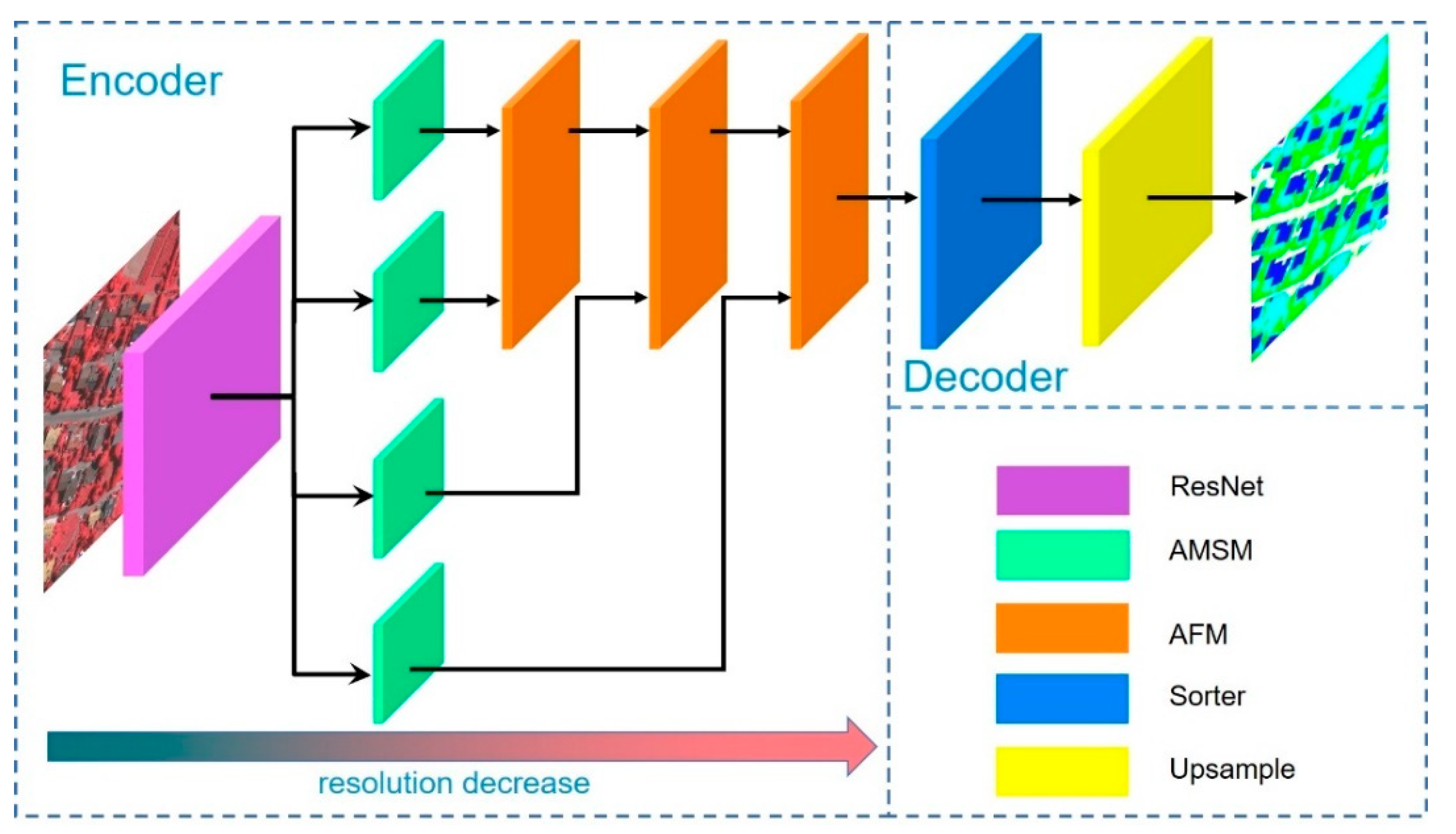
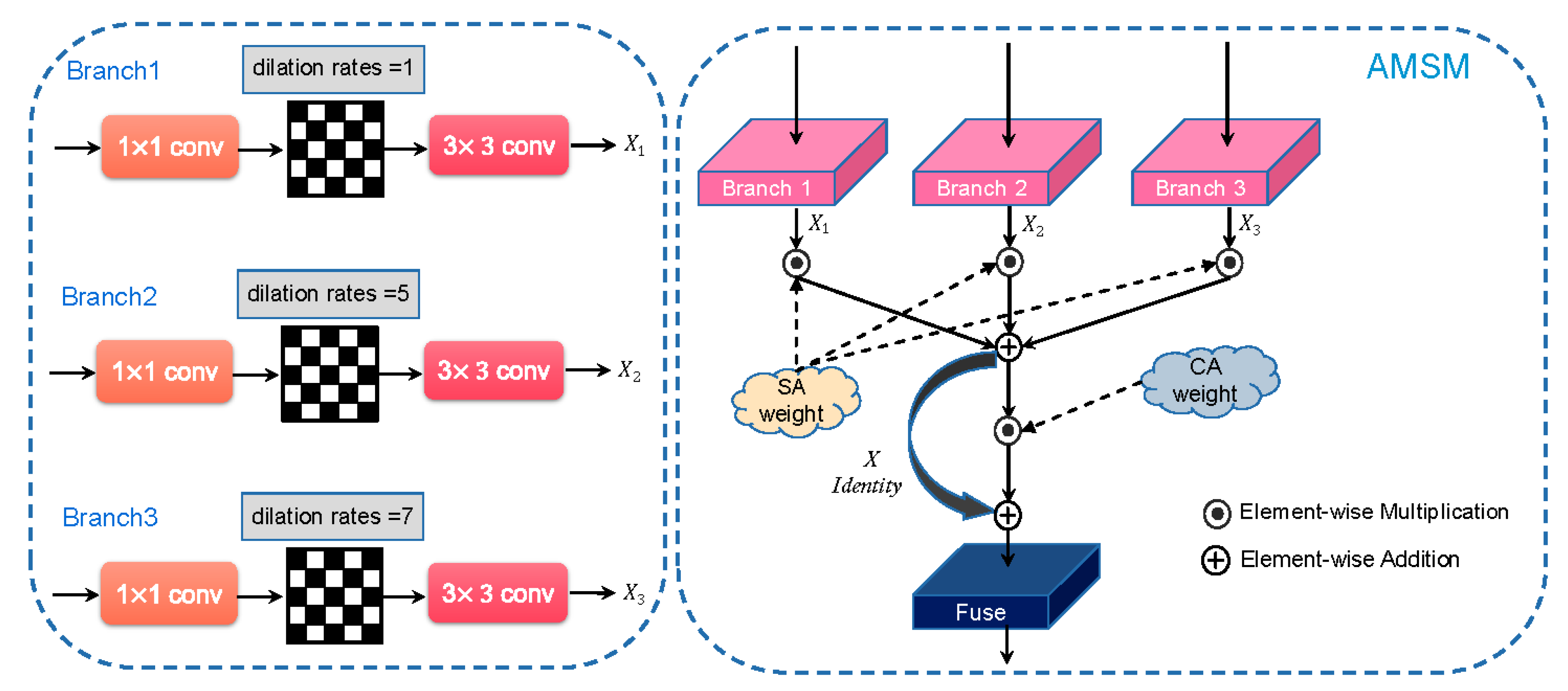
A novel multi-scale fusion module—ASMS (Adaptive Multi-Scale Module) module is proposed, which can adaptively fuse multi-scale features from different branches according to the size characteristics of remote sensing images and has a better segmentation effect in the data sets with complex and variable object sizes.
(2)
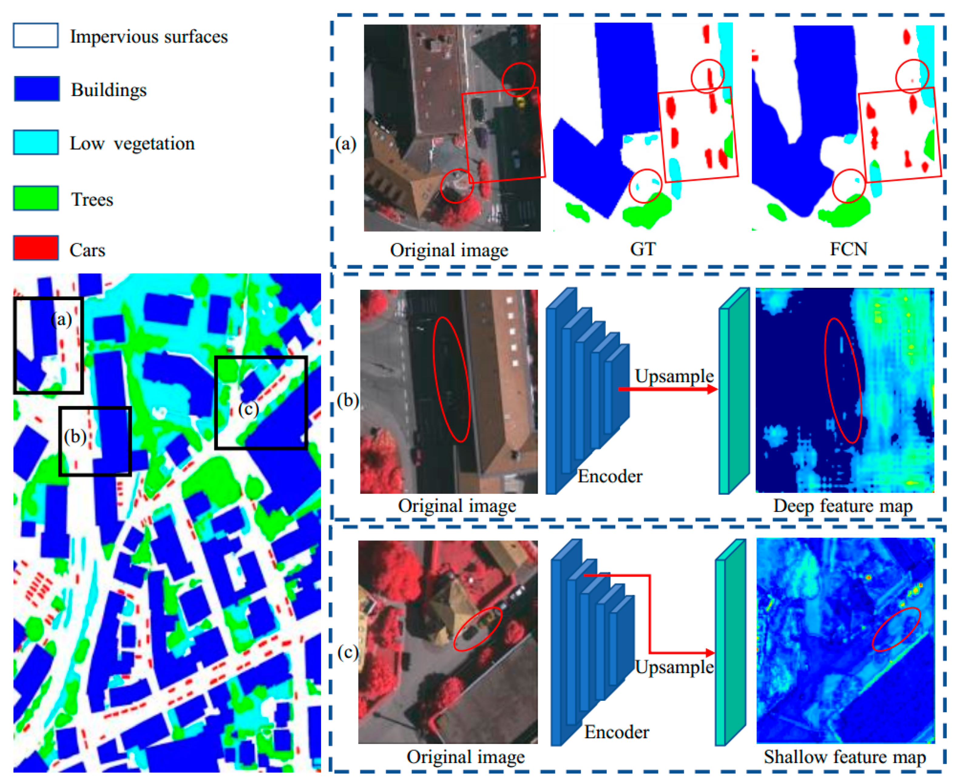
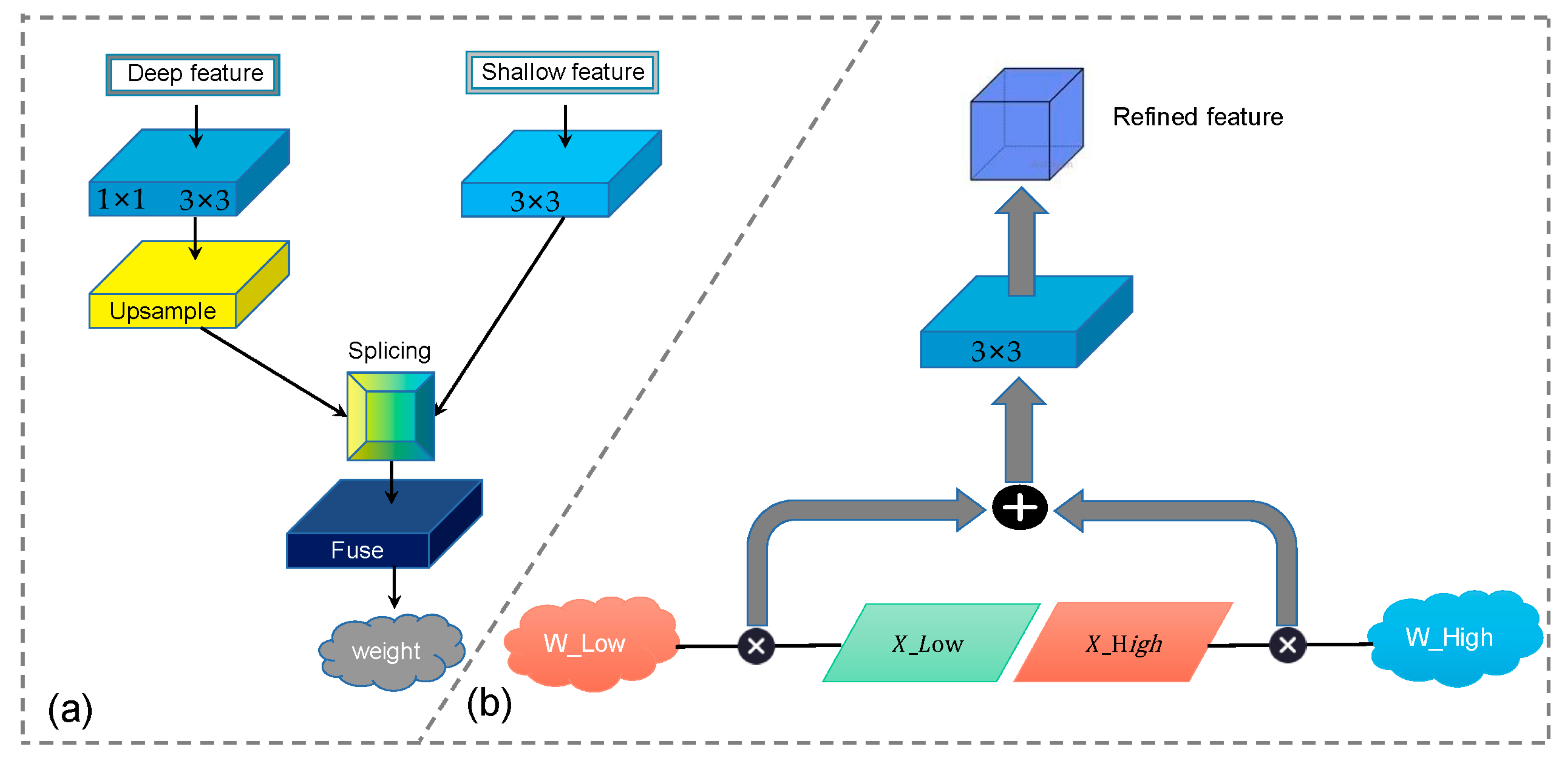
We designed an AFM (Adaptive Fuse Module) that can filter and extract shallow information of remote sensing images. This module can combine the shallow and deep feature information effectively. After obtaining the weights of shallow and deep layers, these weights are multiplied by the original weight of the feature map to emphasize the useful information in the shallow feature map and suppress useless noise. So that the deep feature map can obtain more accurate detailed information.
(3)
A new type of network structure-Adaptive Weighted Network (AWNet) is proposed, which is a network structure embedded with AMSM and AFM. AWNet achieved one of the best accuracies on the ISPRS Vaigingen data set, reaching an overall accuracy of 88.35%.

2. Related work

In this part, we introduce the development of semantic segmentation structure and attention mechanism [16] in order to better discuss our work.

2.1. Semantic Segmentation

In recent years, with the development of deep learning and the computing power of graphics processing units, semantic segmentation has also made considerable progress. In 2015, FCN replaced the fully connected layer of the classic classification network with a convolutional layer and achieved the end-to-end training [6], which became the pioneering work of semantic segmentation.
Later, on this basis, DeepLabv3+ [10], MSCI [17], SPGNet [18], RefineNet [19], and DFN [20] all adopted encoder-decoder structure for dense prediction. Among them, both Refinenet and Global Convolutional Networks (GCNS) [21] have successively reached the most advanced performance. Gradually, the application of semantic segmentation in multi-scale has also made new progress. In order to deal with various scales and deformations of segmented objects, people use Deformable convolutional networks (DCN) [22] and the scale-adaptive convolutions (SAC) [23] model to improve the standard convolution operator. Soon after this, CRF-RNN [24] and DPN [25] used the graph model for semantic segmentation. In order to capture and match the semantic relationship between adjacent pixels in the label space, AAF [26], using adversarial learning, achieves this goal. BiSeNet [27] is applied with real-time semantic segmentation. DenseDecoder [28] built a functional-level remote jump connection on the cascade architecture for the first time, which further improved the effect of semantic segmentation. Later, CE2P [29] proposed a network structure that can achieve both edge detection and computing context embedding, which is also an efficient and concise framework. Obviously, semantic segmentation has made significant progress in various fields.

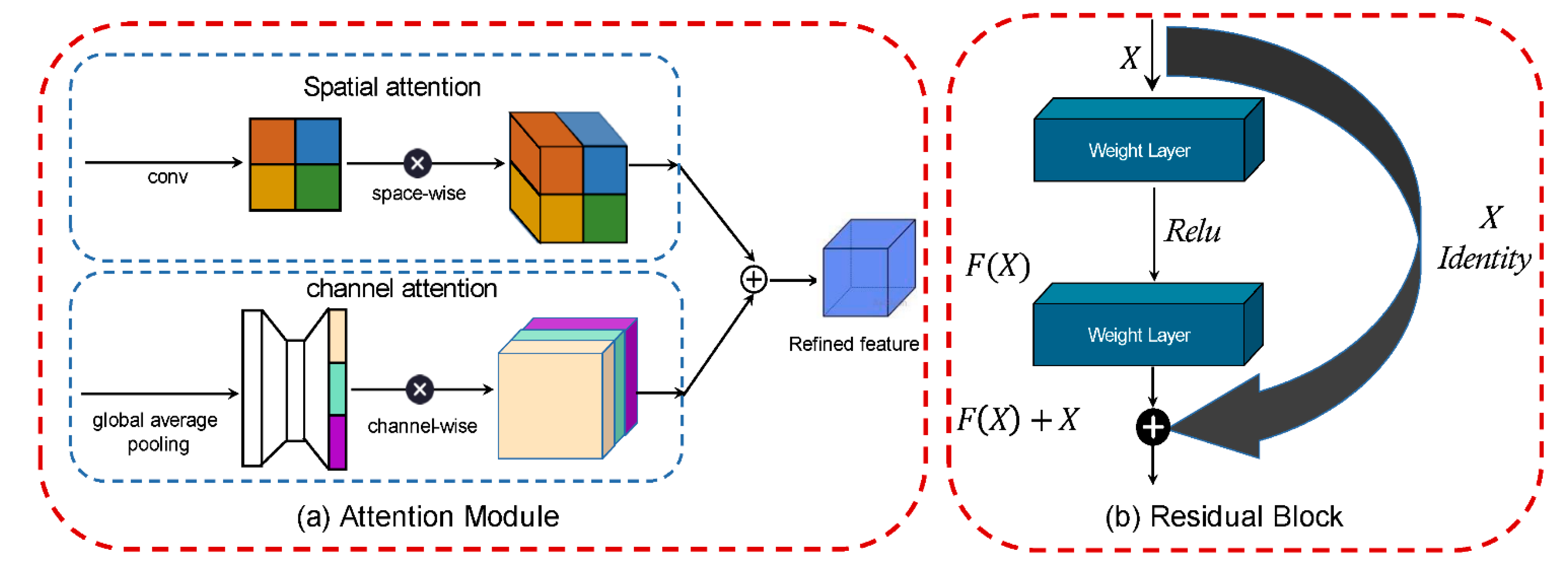
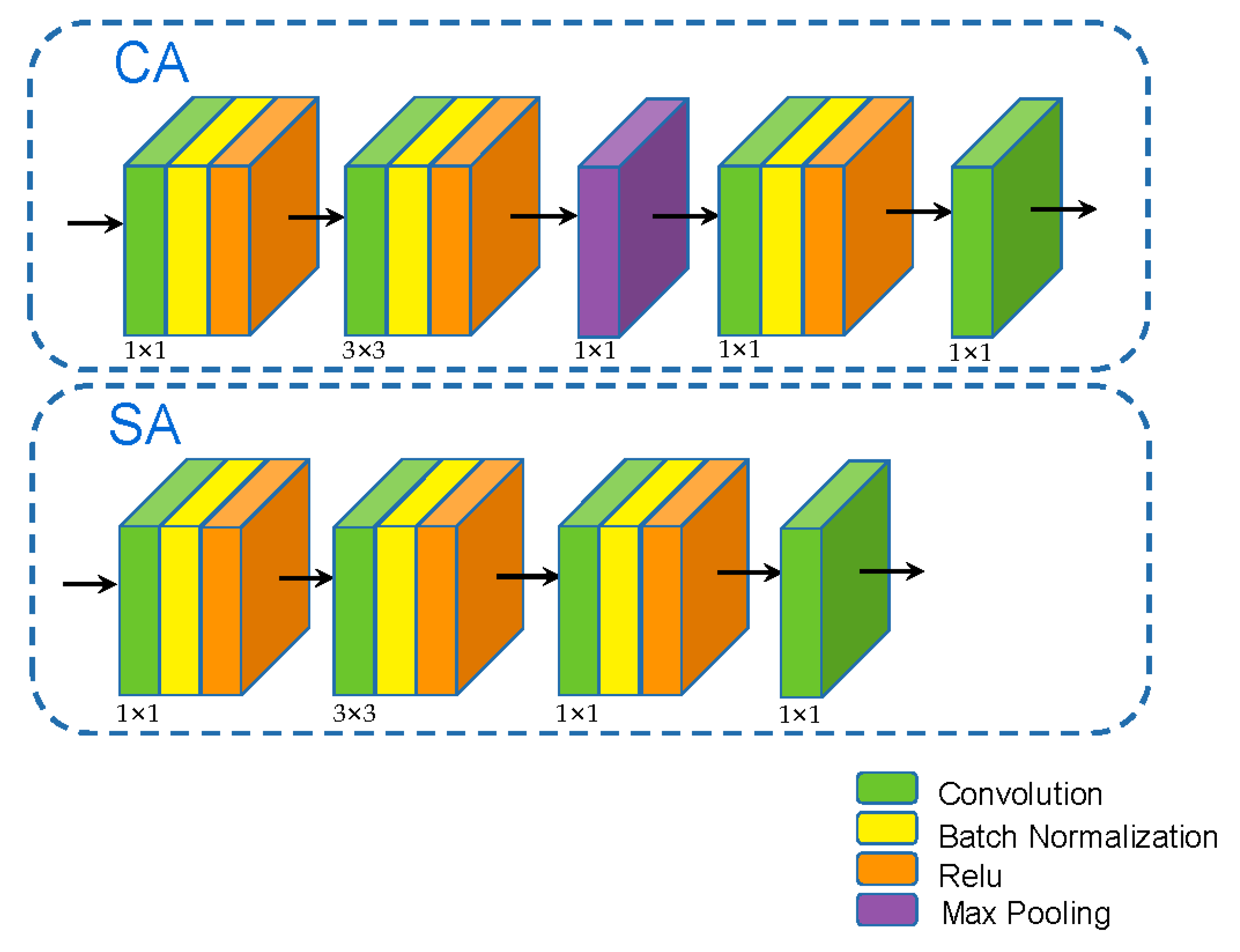
2.2. Attention Module

At present, the attention mechanism has been widely used in computer vision and natural language processing. The attention mechanism module appeared in people’s vision. This is a landmark innovative design, which contains three parts: squeeze, stimulation and attention. For multi-label classification tasks, Hao Guo et al. used attention consistency [30] to make up for the defects of data augmentation in image classification tasks. This model adopts a dual-branch structure and uses two heat maps generated by CAM [31] to achieve the effect of still focusing on the same part after data augmentation. Subsequently, in order to realize the positioning of the shared objects between the images, Bo Li, et al. set the update gate and reset gate [32] so as to continuously update the hidden unit to integrate the information of all images, and then return Parameters to guide the generation of predicted values for each sample. For multi-task learning, Liu S et al. adapted an attention to each task as a feature selector [33], making it possible to extract specific features of each task. Lu, Xiankai et al. proposed a co-attention [34] module, which aligns adjacent frames and then integrates the information between adjacent frames to achieve unsupervised video object segmentation. For the target positioning task, although each channel can respond to a specific object, the noise of a single object is too large. Heliang Zheng, et al. [35] use the idea of self-attention, regard each channel as a spatial attention map, make it corresponding to a specified part, and realize the adaptive and unsupervised positioning of the region of each part of the object.

2.3. Spatial Pyramid Pooling and Atrous Convolution

In the previous CNN structure, the input of the convolutional neural network can only input pictures of a fixed size, which makes it difficult to meet the needs of modern computer vision. In order to realize the recognition of multi-scale objects, people proposed spatial pyramid pooling (SPP) on the basis of a convolutional neural network [26]. The SPP structure can use different sizes of the same image as input and output the same pooling feature. Moreover, regardless of the input of any size of the image, the image after SPP can produce a fixed size of output. Finally, all the segmentation results are merged to obtain the semantic segmentation result of the original input image.
Later, the concept of parallel sampling was proposed, and an upgraded version of SPP, ASPP, appeared. In this module, the input image can be sampled in parallel with irregular convolution. After each channel is sampled and pixels are added, the results obtained by irregular convolution of each branch are fused to obtain the final prediction result. ASPP also makes full use of the atrous convolution, effectively expanding the receptive field without increasing the amount of parameters and merging more context information. Hollow convolution is a convolution method born in the field of image segmentation. It proposes the characteristics of the input image through a convolutional neural network, and expands the receptive field, while merging to reduce the image size. Then, it restores the image size by upsampling to generate an output image. However, due to the limitations of the upsampling algorithm, many details will be lost with the merge. This problem is solved by expanding the receptive field. There is an important parameter (r) in the atrous convolution. When r = 1, it is a standard convolution process. When r > 1, every (r − 1) pixels will be sampled once. This idea is similar to that of dilated convolution [13].

3. Materials and Methods

Inspired by the attention mechanism [30], we proposed the AMSM module and the AFM module. In this part, we mainly describe the realization of this specific model. First, we introduced the overall architecture used to test both modules, namely the AWNet workflow. After that, the network architecture of the AMSM module is introduced. Finally, the construction principle of the AFM module is explained.

3.1. Overview

As shown in Figure 2, this network is mainly composed of three parts: ResNet preprocessing encoder based on residual block; AMSM; and AFM of attention module and upsampling block. The encoder-decoder structure is one of the most common structures in segmented networks. It is possible to extract effective global and local information by extracting high-resolution remote sensing images. In the encoder part, the network ensures the effective use of semantic and spatial information. First, we output different levels of semantic information through the Resnet101 [36] network. Then, we used AMSM stacked in the encoder part as a feature extractor. Each level performs multi-scale feature extraction on the semantic information of the fixed-dimensional image to ensure that it can be adaptively fused with the change of the image scale. Then, we used AFM to fully integrate deep and shallow semantic information. This module is a better feature extractor, designed to ensure consistent resolution. After the processing was over, the number of channels of the feature map was reduced to the same number of categories. The decoder part uses upsampling to restore the feature map to the original image size and output the final result. Facts have proven that our proposed AWNet, a new network deconstruction that combines AMSM and AFM, is very effective and practical in processing the spatial and semantic information of remote sensing images.
At the same time, it is important to consider low-level details while preserving high-level semantic information in order to achieve more accurate semantic segmentation. Especially for high-resolution remote sensing images, it has more detailed information than natural images. In general, deeper networks will get better functionality. However, due to the disappearance of the gradient, the training results will be unsatisfactory, as shown in Figure 1. This problem can be solved using residual neural networks, as shown in Figure 3. The mechanism of residual blocks can be expressed by the following formula:
  Y L = H ( X L ) + F ( X L , W L )
X L + 1 = f ( Y L )
Here, X L and X L + 1 represent input or output residual blocks, and each residual block may contain a multi-layer structure. The residual function can be represented by F , which is obtained by the weight W L and the output X L of the previous layer. Here H ( X L ) is the input of a certain layer of neural network. If the expected output, Y L , is a complex latent mapping, such model training is more difficult. The input H ( X L ) of the neural network of this layer can be directly used as the initial result of the output of this layer to effectively improve the training effect. f ( x ) is the activation function of the linear unit Relu.

3.2. Pretreatment

Before the formal training, we used the pre-trained expanded ResNet-101 [37] to preprocess the input image to extract semantic features in the global scope. The entire semantic input stream can be expressed as:
F s = S θ ( I )
Here I R H × W × 3 represents the original input remote sensing image. W and H represent the width and height of the input image, respectively. θ respectively represents the parameters of the semantic input stream. F R H 8 × W 8 × 2048 represents the semantic map of the output feature map. S θ ( I ) represents the preprocessing process of ResNet semantic flow under the θ conditions. The independent variable I is the original semantic input stream.

3.3. Adaptive Multi-Scale Module (AMSM)

Because the ASPP structure directly integrates multiple scales (different atrous rates), it does not guarantee the adaptive fusion of the branch information, which will lead to inconsistencies within the class. In order to solve the problem of differences in features corresponding to objects with the same label, we designed the AMSM structure to adaptively optimize features by using the attention mechanism.
Figure 4 shows this structure in detail. It combines a spatial attention module and channel attention module. In order to fully enhance the characterization effect of the module, the two modules are combined together. The structure consists of three parallel structures, and the weights obtained using the spatial attention mechanism are then multiplied by the output of the parallel structure pixel by pixel. After that, the residual network module is used to multiply the feature graph pixel by pixel with the weight generated by multi-channel attention. Finally, the feature map is restored to the size of the original input image through the Fuse block (composed of 1 × 1 convolutional layer and 3 × 3 convolutional layer in series).
For the three branches of AMSM, each branch corresponds to a different void rate so as to obtain different weights according to the size of the remote sensing image. The input image passes through a spatial attention module. The number of channels output by this module is three. We assumed that the output X i (i = 1, 2, 3) is the feature of each layer, and the output results of the three channels are regarded as the weights of their respective spaces. Then, we used the spatial attention mechanism to generate the weight SA weight [37], as shown in the right part of Figure 4. After getting the spatial attention weight, it was multiplied by each branch to achieve fusion. Figure 5 shows the process of obtaining spatial attention weights and channel attention weights. The input image passes through a channel attention module, and the channel attention is used for further screening, assuming that each layer outputs Y i (i = 1, 2). Then the fusion feature N i of each spatial attention channel is
N i = X i Y i
Further, the three-layer output is added and fused, and f ( X ) is the jump connection.
M = Y i ( N 1 + N 2 + N 3 ) + f ( X )
Finally, the output results are convolved with the residual structure through two layers to achieve the effect of reducing the number of channels.
It is worth mentioning that AMSM is very simple to use and does not require too many additional parameters or computations. For various network models, there are two common embedding methods. One is to add AMSM after each convolution layer of some network structure. The other is to add AMSM between the two blocks of the remaining network.
The channel attention module generates channel attention feature maps by using channel connections between features. Each channel in the feature map is treated as a feature detector. The focus of the channel attention mechanism is mainly on what is meaningful in the input image. Channel attention uses two common methods to aggregate spatial information, namely max pooling and average pooling operations.
The spatial attention is different from the channel attention above, it mainly focuses on the position information of the input image. It first uses average pooling and maximum pooling to obtain two different feature descriptions. In the channel dimension, the two pooled feature descriptions are integrated. Finally, we used the concat operation to generate the spatial attention map.

3.4. Adaptive Fuse Module (AFM)

The input of AFM is a feature map of semantic information from different convolution kernel sizes. The architecture of Adaptive Fuse Module is shown in Figure 6, and the numbers marked in the figure are the size of the convolution kernel in the block. As can be seen, in this module, we got feature maps with different resolutions from two branches, namely, deep and shallow feature maps. When the combined feature map is obtained, it is necessary to ensure that the two branches maintain the same size, so it is necessary to carry out upsampling after the deep feature map to restore the feature map size. Shallow feature maps contain useful edge information and details but also annoying noise. Therefore, we filtered the shallow feature map with the help of deep features, filtering out the unnecessary noise information and only retaining the required details; we then performed the fusion operation. The weight generation process is shown in Figure 6a. The Fuse block after the fusion of the deep and shallow feature maps is three 1 × 1 convolutional layers in series. It should be noted that these feature maps will be added pixel by pixel instead of simple merging.
There are many reasons why we chose this method, including the following main reasons. First, we can ensure that the weights of the two branches can be easily obtained after data normalization. In addition, the calculation cost can be reduced while the size is uniform. However, the feature processed in this form is not suitable for calculation and extraction. Therefore, in order to better aggregate spatial information, we add a convolution layer after fusion to solve this problem. We no longer use a single branch to calculate the global semantic information and spatial information. It is proposed to use multi-scale to collect weights from deep and shallow layers. The final feature map will be the sum of the feature maps of the two branches, as shown in Figure 6b.

4. Experiments

To verify the validity of our model, we conducted a series of experiments using the ISPRS Vaihingen dataset. The data sets are available from http://www2.isprs.org/commissions/comm3/wg4/2d-sem-label-vaihingen.html (accessed date 25 November 2020). In A, we introduced the dataset and measurement index; in B, we introduced the preprocessing method of the dataset; and in C, we introduced the specific hyperparameters used in the experiment.
The ISPRS Vaihingen dataset contains a total of 33 graph blocks, and the dataset can be split to represent the semantic markup of each graph block. Figure 7 shows the input image of a sample in the ISPRS dataset and the ground truth corresponding to this image.
We conducted a lot of experiments on the ISPRS Vaihingen dataset to evaluate the algorithm model we proposed. The following experiments will be carried out with this as a sample.

4.1. Experiments Sets

(1) Database Sets
The ISPRS Vaihingen dataset is composed of 33 aerial images, as shown in Table 1. These images have a spatial resolution of 9 cm and are collected from an area of 1.38 square kilometers. In this data set, the average size of each picture is 2494*2064 pixels, and each picture has three bands of green (G), near infrared (NIR), and red (R). It is worth mentioning that, in order to achieve a generalized template, we did not use DSM data in the experiments conducted in this article. The data set is divided into training data (ID 1, 3, 11, 13, 15, 17, 21, 26, 28, 30, 32, 34) and verification data (ID 5, 7, 23, 37). Meanwhile, in our study, all the pixels in the image are divided into six categories, which are white impermeable surface, blue building, cyan low vegetation, green tree, yellow car, and red background, as shown in Figure 8.
(2) Evaluation indicators
In order to better evaluate our model, we used F1-score and Overall Accuracy (OA) as network accuracy evaluation indicators. The two classification indicators are briefly introduced below.
F1-score is a very important indicator in classification problems. This indicator takes into account both the precision rate and the recall rate, and uses the percentage of pixels that predict the correct category as the overall accuracy. Among them, both values are between 0 and 1. The closer the value is to 1, the higher the accuracy. The two parameters used to calculate F1-score involve recall and accuracy, which are defined as:
r e c a l l ( c ) = T P C × 100 %
p r e c i s i o n ( c ) = T P C × 100
Among them, TP represents the number of categories C correctly predicted by the model. P represents the total number of pixels in the sample predicted by the model as category C, and C is the total number of pixels in the sample. When it is necessary to consider both the accuracy rate and the recall rate, the model’s F1-score index can be used to judge the pros and cons of the model. F1-socre also considers the precision and recall of the model, which is defined as follows:
F 1 = 2 × p r e c i s i o n ( C ) × r e c a l l ( C ) p r e c i s i o n ( C ) + r e c a l l ( C ) × 100 %
Among them, precision represents the accuracy of the model, which is the proportion of correct results in the total results predicted by the model. Recall is the recall rate of the model, which is the percentage of correct results predicted by the model in the true value label of the sample. F1 is the harmonic average of precision and recall. Therefore, F1-score will only be high when the precision and recall indicators are balanced.
Overall Accuracy represents the proportion of samples that are correctly classified in all samples. This indicator reflects the correctness of the overall classification of the map and is a rough overall measure.
The overall accuracy is the percentage of pixels with the correct class predicted, and the accuracy is defined as
A c c u r a c y = T A × 100 %
In this formula, T represents the number of pixels that predict the correct category, and A is the total number of all pixels.
For each category, the average F1 score is achieved by calculating all F1 scores to achieve a fair evaluation model. It is worth noting that the higher the F1 score, the better the model evaluation result.

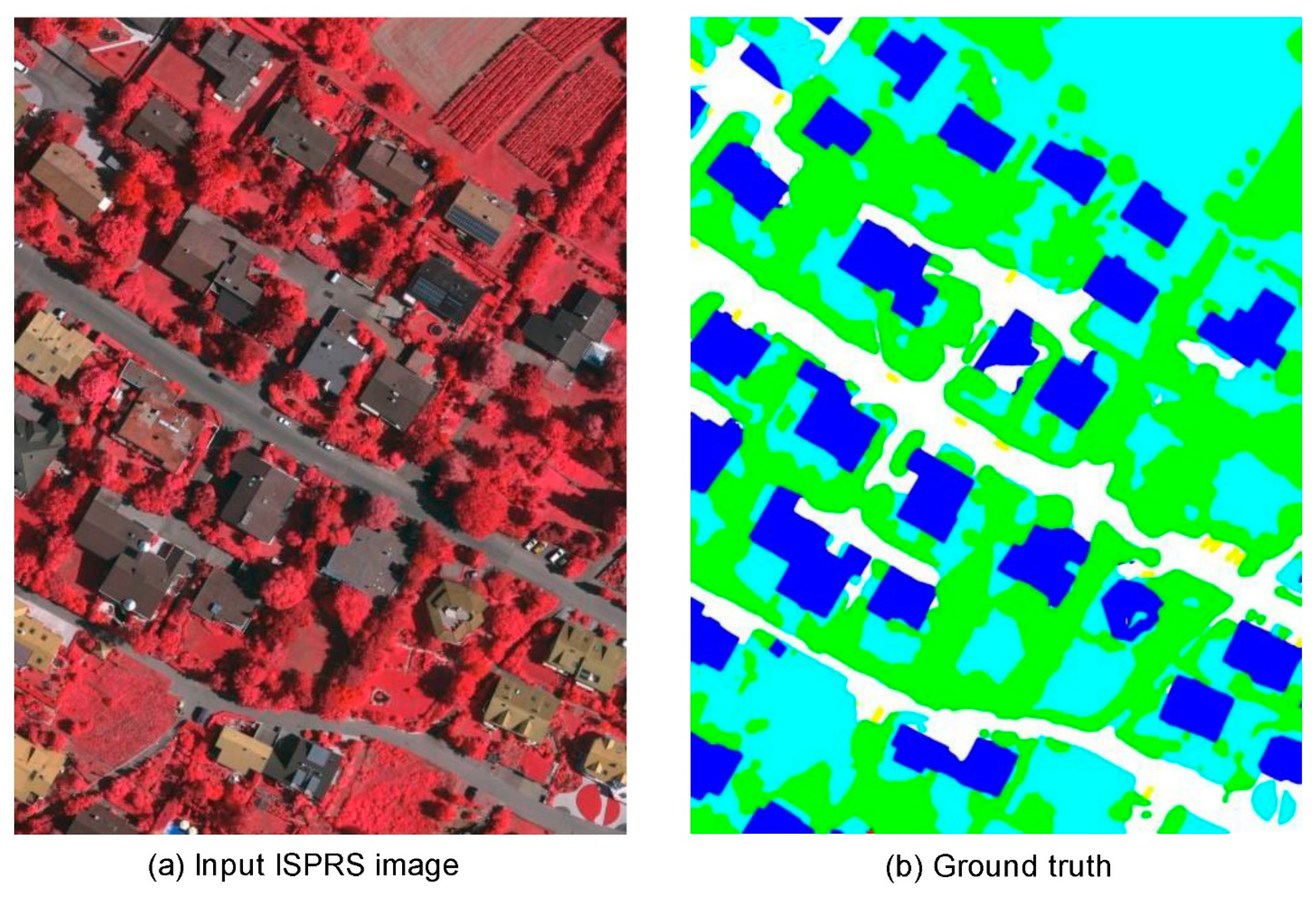
4.2. Data Set Preprocessing

Due to the limited Graphic Processing Unit (GPU) memory, we cut the input image of the model to a fixed pixel size through a sliding window and, then, input it into our model to train and verify the images in the dataset. Similar to the current mainstream processing methods, we used some of the more common data enhancement strategies to achieve data enhancement, such as Gaussian blur, image rotation, random cropping, horizontal flip, vertical flip, 90-degree rotation, grid mask, etc. These methods not only play a role in data enhancement but also prevent the occurrence of over-fitting to a certain extent.

4.3. Implementation

We developed the following training strategy. For the optimizer used, we chose ADAM’s optimizer and set the parameters of the optimizer according to the suggestions, setting the initial learning rate as 1e-3. The model was trained on a single NVIDIA Tesla V100. We set the batch size to 3, trained a total of 50 epochs, and when the verification loss started to stop reducing, we would stop the training. In order to reduce the vibration of the model in the later period of training, we adopted the adaptive learning rate decline strategy. We used U-Net with ResNet-101 as out baseline. Similar to the method used in similar studies, weighted cross entropy function is used to train the whole model. We implemented our network using PyTorch, where the learning rate was initialized to 1e-3 when the validation loss was saturated, and we stopped training when the validation loss function failed to decrease. After setting the above parameters, we trained and tested AWNet. The training of the model lasted about 50 hours, and the test lasted about 20 minutes.

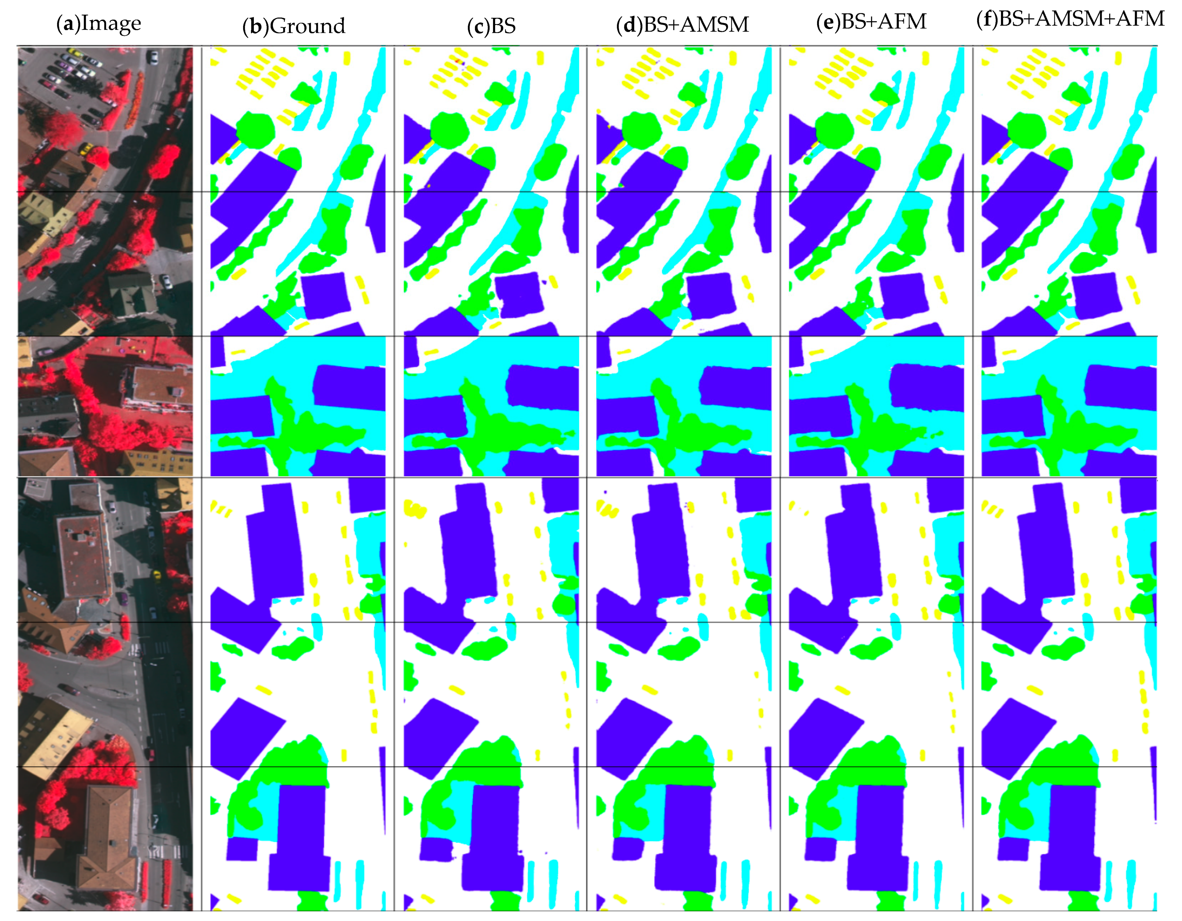
4.4. Ablation Study for Relation Modules

We evaluated each component of the model, used ResNet-101 as our baseline, and added AFM and AMSM to enhance the consistency of the model. In order to verify the performance of the various models we proposed, we conducted a series of ablation experiments. The experimental results of different models in the Vaihingen data set are presented in Table 2.
The overall accuracy rate of ResNet101 + AMSM + AFM in ablation experiments is 88.35%, which is better than ResNet, ResNet + AMSM, and ResNet + AFM. As shown in Figure 9, in the comparison with ground truth, we can see that when only the baseline is used for segmentation, the adhesion between two similar objects that are close in distance is more obvious, and there is obvious noise at the edge. After adding AMSM or AFM, the adhesion phenomenon was reduced, and the independence of the object was improved. See Figure 9f again. After using AMSM and AFM at the same time, there is almost no adhesion between the edges between two objects that are close to each other. The noise at the edge of each object is also significantly reduced, making the boundary of the segmentation result clearer.

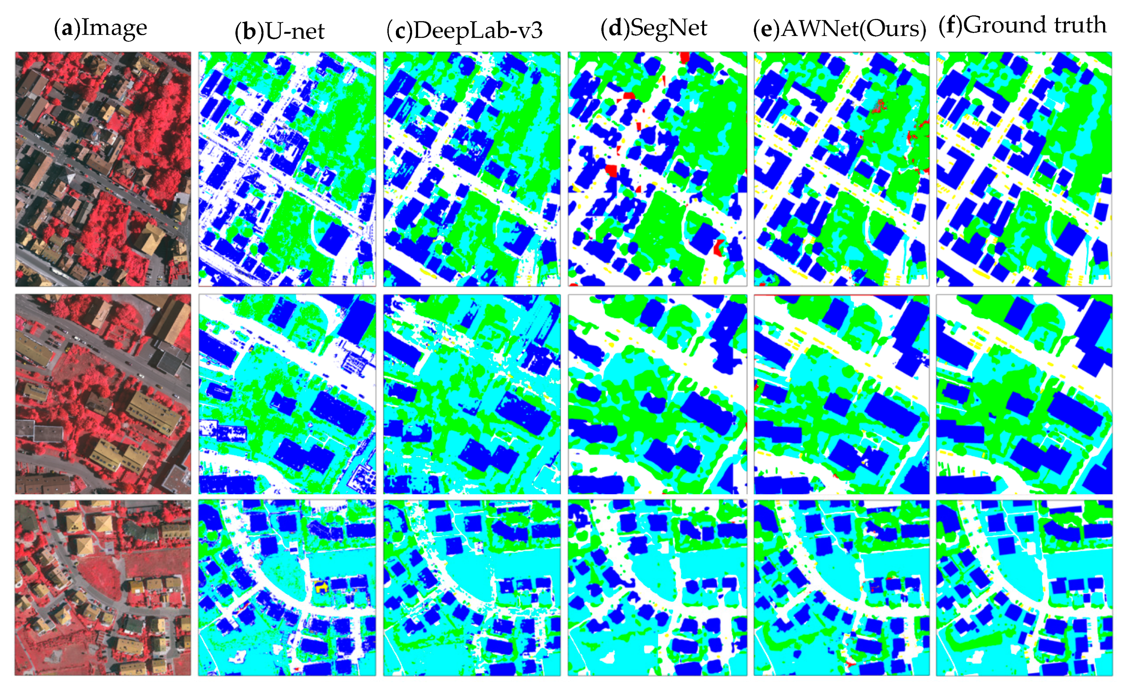
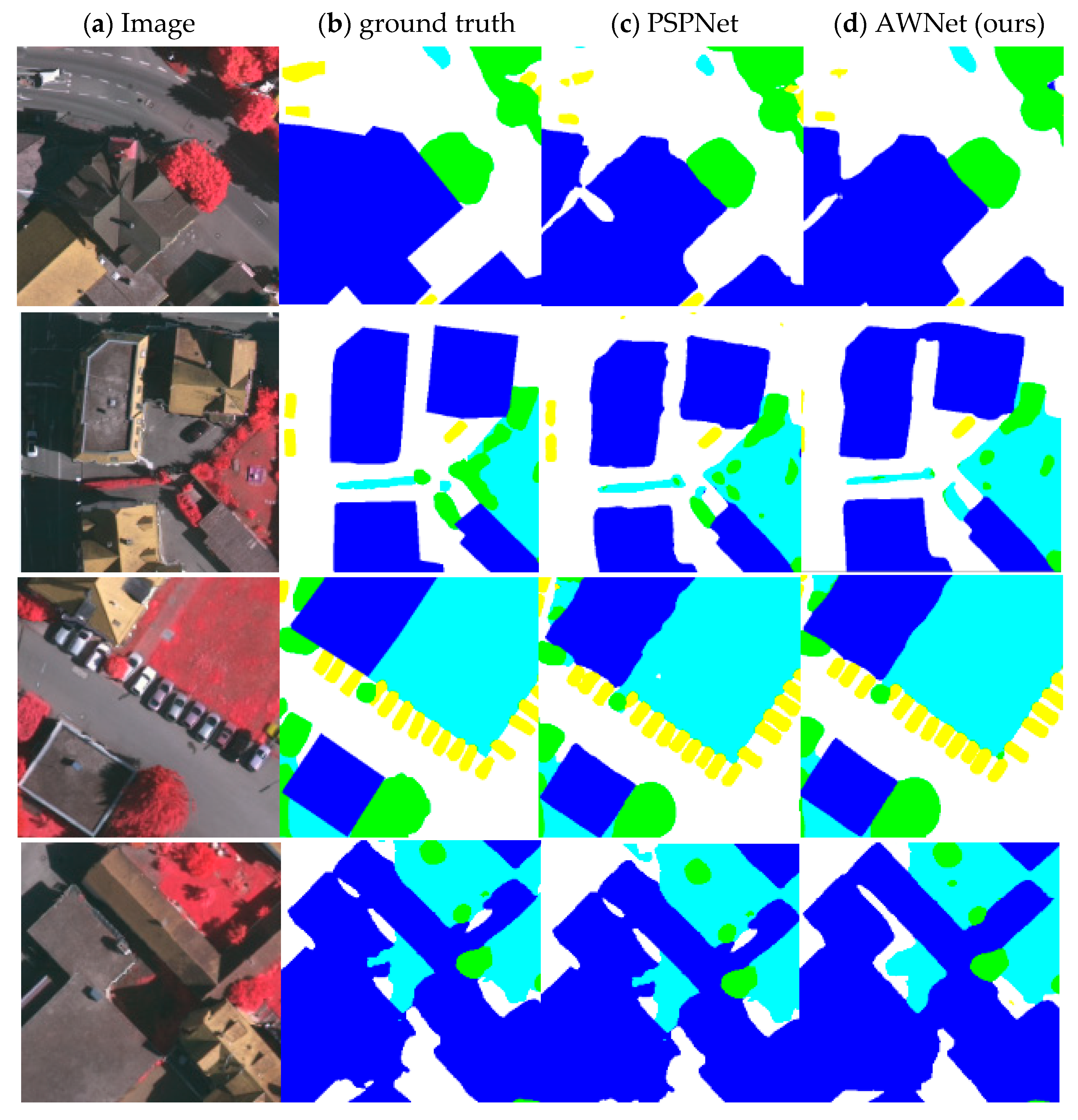
4.5. Comparing with Existing Works

In order to make a more comprehensive evaluation of our research, we first tested the model with five landmark networks [6,7,14,15,38], and the test results obtained are shown in Table 3. The output image is shown in Figure 10. At the same time, we also compared our model with five existing models based on basic network improvements, including FCN with fully connected CRF (FCN-dcrf), spatial propagation CNN (SCNN) [39], FCN with atrus convolution (extensed FCN) [9], FCN with feature remake (FCN-FR) [40], convolutional neural network (CNN-FPL) with patch labeling learning through learning upsampling [41], and VGG16 is the PSPNet of the backbone network [42], and the test results are shown in Table 4.
The numerical results of the Vaihingen data set are shown in Table 3 and Table 4. The results show that whether it is a landmark classic network or an improved network based on the classic network, our model is superior to other methods in terms of F1 average score and overall accuracy. Specifically, for example, compared with FCN-dCRF and SCNN, the average F1 score of our proposed network increased by 1.70% and 1.92%, respectively, which verified the high performance of the spatial relationship module in our network. It shows that the integration of AMSM and AFM relationship modules is effective.
Our model has obvious advantages in dealing with small objects. Specifically, the “car” category is a category that is difficult to handle in the Vaihingen dataset because, compared with other categories, “car” is a relatively small object. As shown in Table 3 and Figure 11, the number of pixels in other categories is much more than the number of pixels in the “car” category, and there are large differences in objects between this category. For example, the diversity of car colors in the image also leads to huge differences within the category. Our proposed method achieves an accuracy of 82.22% in the car category, which is significantly higher than other models, which proves the effect of our method on small targets.
In addition, the qualitative results are shown in Figure 11. For the first line, although the low-vegetation area contains complex local context information and is easily misidentified, due to its powerful function, our network can obtain more accurate results, compared with other methods, to solve the problem of vision blurring [43,44,45] by using global relations, and the phenomenon of category misclassification [46] is greatly reduced. In addition, the edge of our model is clearer and more coherent, which proves that the model has the function of eliminating outliers, and the noise in the detail information has less impact on the result.

5. Conclusions and Future Work

In this paper, we propose two kinds of effective network modules to solve the noise and classification problems in remote sensing images. Adaptive Multi-Scale Module (AMSM) and Adaptive Fuse Module (AFM). Among them, the Adaptive Multi-Scale Module (AMSM) can adaptively generate spatial weight, which has a better segmentation effect in the data set with complex and variable object size. The AFM (Adaptive Fuse Module) module, which can filter and extract shallow information of remote sensing images, is also designed. This module can effectively remove the noise information in the shallow layer feature image and make up for the details with better robustness in the deep layer feature image. Both relationship modules learn the global relationship information between the target and the feature graph. Verified on the Vaihingen dataset, we used the network of two relationship modules to better identify smaller targets while still maintaining good overall accuracy. Moreover, the multi-scale convolutional feature network of AMSM and AFM is superior to other models in terms of vision and numerical value. AWNet’s F1 Score reached OA and reached 88.35%. However, our understanding of how these two modules deal with segmentation problems in remote sensing images is not yet in place, and further research is needed.

Author Contributions

Conceptualization, Yifan Liu and Junke Chen; methodology, Yifan Liu, Qigang Zhu; validation, Yifan Liu, Junke Chen, Gang Lu and Feng Cao; formal analysis, Yifan Liu and Qigang Zhu; investigation, Yifan Liu, Gang Lu and Feng Cao; data curation, Yifan Liu and Gang Lu; writing—original draft preparation, Yifan Liu and Junke Chen; writing—review and editing, Yifan Liu, Junke Chen, Gang Lu, Qigang Zhu and Feng Cao; visualization, Yifan Liu and Junke Chen; project administration, Yifan Liu; All authors have read and agreed to the published version of the manuscript.

Funding

This project is funded by the Provincial and School-level Educational Reform Project-Communication Engineering CDIO Talent Training (Project Number: 310301815) and Excellent Teaching Team Project (Project Number: 310302202).

Institutional Review Board Statement

Not applicable.

Informed Consent Statement

Not applicable.

Data Availability Statement

The data presented in this study are openly available in http://www2.isprs.org/commissions/comm3/wg4/2d-sem-label-vaihingen.html (accessed on 25 November 2020).

Acknowledgments

I sincerely thank Zhang Shuaishuai and Yuan Yulei for answering my questions patiently and giving me great help during the writing process. In particular, on behalf of all the authors, I would like to thank Zhang Shuaishuai again for vividly providing me with ideas for revising the paper and replying to the reviewers’ opinions during the review period. At the same time, I also sincerely thank other teachers on the Jinan campus of Shandong University of Science and Technology for their support and encouragement in all aspects, including Han Wei and Han Bing from the Study Group Department; Chen Fangzhou, Zhang Hongbin, and Zhang Hongbin from the Department of Electrical Information; and Li Wei, Liu Hao, and Xu Haowen, who has always encouraged and supported me.

Conflicts of Interest

The authors declare no conflict of interest.

Abbreviations

The following abbreviations are used in this manuscript:
AMSMAdaptive Multi-Scale Module
AFMAdaptive Fuse Module
AWNetAdaptive Weighted Network
ASPPAtrous Spatial Pyramid Pooling
BSBaseLine
RGBRed–Green–Blue
CNNConvolutional Neural Network
OAOverall Accuracy

References

  1. Wen, D.; Huang, X.; Liu, H.; Liao, W.; Zhang, L. Semantic Classification of Urban Trees Using Very High Resolution Satellite Imagery. IEEE J. Sel. Top. Appl. Earth Obs. Remote Sens. 2017, 10, 1413–1424. [Google Scholar] [CrossRef]
  2. Shi, Y.; Qi, Z.; Liu, X.; Niu, N.; Zhang, H. Urban Land Use and Land Cover Classification Using Multisource Remote Sensing Images and Social Media Data. Remote Sens. 2019, 11, 2719. [Google Scholar] [CrossRef] [Green Version]
  3. Matikainen, L.; Karila, K. Segment-Based Land Cover Mapping of a Suburban Area—Comparison of High-Resolution Remotely Sensed Datasets Using Classification Trees and Test Field Points. Remote Sens. 2011, 3, 1777–1804. [Google Scholar] [CrossRef] [Green Version]
  4. Xu, S.; Pan, X.; Li, E.; Wu, B.; Bu, S.; Dong, W.; Xiang, S.; Zhang, X. Automatic Building Rooftop Extraction from Aerial Images via Hierarchical RGB-D Priors. IEEE Trans. Geosci. Remote Sens. 2018, 56, 7369–7387. [Google Scholar] [CrossRef]
  5. Liu, W.; Yang, M.; Xie, M.; Guo, Z.; Li, E.; Zhang, L.; Pei, T.; Wang, D. Accurate Building Extraction from Fused DSM and UAV Images Using a Chain Fully Convolutional Neural Network. Remote Sens. 2019, 11, 2912. [Google Scholar] [CrossRef] [Green Version]
  6. Long, J.; Shelhamer, E.; Darrell, T. Fully Convolutional Networks for Semantic Segmentation. In Proceedings of the IEEE Conference on Computer Vision and Pattern Recognition (CVPR), Boston, MA, USA, 7–12 June 2015. [Google Scholar]
  7. Ronneberger, O.; Fischer, P.; Brox, T. U-Net: Convolutional Networks for Biomedical Image Segmentation. In Proceedings of the International Conference on Medical Image Computing and Computer-Assisted Intervention, Munich, Germany, 5–9 October 2015; pp. 234–241. [Google Scholar]
  8. Zhou, J.; Hao, M.; Zhang, D.; Zou, P.; Zhang, W. Fusion PSPnet Image Segmentation Based Method for Multi-Focus Image Fusion. IEEE Photon. J. 2019, 11, 1–12. [Google Scholar] [CrossRef]
  9. Chen, L.-C.; Papandreou, G.; Kokkinos, I.; Murphy, K.; Yuille, A.L. DeepLab: Semantic Image Segmentation with Deep Convolutional Nets, Atrous Convolution, and Fully Connected CRFs. IEEE Trans. Pattern Anal. Mach. Intell. 2017, 40, 834–848. [Google Scholar] [CrossRef]
  10. Chen, L.; Zhu, Y.; Papandreou, G.; Schroff, F.; Adam, H. Encoder-Decoder with Atrous Separable Convolution for Semantic Image Segmentation. In Proceedings of the European Conference on Computer Vision (ECCV), Munich, Germany, 8–14 September 2018. [Google Scholar]
  11. Pan, X.; Gao, L.; Zhang, B.; Yang, F.; Liao, W. High-Resolution Aerial Imagery Semantic Labeling with Dense Pyramid Network. Sensors 2018, 18, 3774. [Google Scholar] [CrossRef] [PubMed] [Green Version]
  12. Yang, F.; Fan, H.; Chu, P.; Blasch, E.; Ling, H. Clustered Object Detection in Aerial Images. In Proceedings of the 2019 IEEE/CVF International Conference on Computer Vision (ICCV), Seoul, Korea, 27 October–2 November 2019; pp. 8310–8319. [Google Scholar]
  13. Woo, S.; Kim, D.; Cho, D.; Kweon, I.S. LinkNet: Relational Embedding for Scene Graph. arXiv 2018, arXiv:1811.06410. [Google Scholar]
  14. Chen, L.C.; Papandreou, G.; Schroff, F.; Adam, H. Rethinking Atrous Convolution for Semantic Image Segmentation. arXiv 2017, arXiv:1706.05587. [Google Scholar]
  15. Badrinarayanan, V.; Kendall, A.; Cipolla, R. SegNet: A Deep Convolutional Encoder-Decoder Architecture for Image Segmentation. IEEE Trans. Pattern Anal. Mach. Intell. 2017, 39, 2481–2495. [Google Scholar] [CrossRef]
  16. Mnih, V.; Heess, N.; Graves, A.; Kavukcuoglu, K. Recurrent Models of Visual Attention. arXiv 2014, arXiv:1406.6247. [Google Scholar]
  17. Lin, D.; Ji, Y.; Lischinski, D.; Cohen-Or, D.; Huang, H. Multi-scale Context Intertwining for Semantic Segmentation. In Proceedings of the European Conference on Computer Vision (ECCV), Munich, Germany, 8–14 September 2018. [Google Scholar]
  18. Cheng, B.; Chen, L.-C.; Wei, Y.; Zhu, Y.; Huang, Z.; Xiong, J.; Huang, T.; Hwu, W.-M.; Shi, H.; Uiuc, U. SPGNet: Semantic Prediction Guidance for Scene Parsing. In Proceedings of the 2019 IEEE/CVF International Conference on Computer Vision (ICCV), Seoul, Korea, 27 October–2 November 2019; pp. 5217–5227. [Google Scholar]
  19. Lin, G.; Milan, A.; Shen, C.; Reid, I. RefineNet: Multi-path refinement networks for high-resolution semantic segmentation. In Proceedings of the 30th IEEE Conference on Computer Vision and Pattern Recognition, Honolulu, HI, USA, 22–25 July 2017; Volume 2017, pp. 5168–5177. [Google Scholar]
  20. Yu, C.; Wang, J.; Peng, C.; Gao, C.; Yu, G.; Sang, N. Learning a Discriminative Feature Network for Semantic Segmentation. In Proceedings of the IEEE Computer Society Conference on Computer Vision and Pattern Recognition, Salt Lake City, UT, USA, 18–22 June 2018; pp. 1857–1866. [Google Scholar]
  21. Kumar, B.V.; Carneiro, G.; Reid, I. Learning Local Image Descriptors with Deep Siamese and Triplet Convolutional Networks by Minimizing Global Loss Functions. In Proceedings of the 2016 IEEE Conference on Computer Vision and Pattern Recognition (CVPR), Las Vegas, NV, USA, 27–30 June 2016; pp. 5385–5394. [Google Scholar]
  22. Dai, J.; Qi, H.; Xiong, Y.; Li, Y.; Zhang, G.; Hu, H.; Wei, Y. Deformable convolutional networks. In Proceedings of the 2017 IEEE International Conference on Computer Vision (ICCV), Venice, Italy, 22 October 2017; pp. 764–773. [Google Scholar]
  23. Zhang, R.; Tang, S.; Zhang, Y.; Li, J.; Yan, S. Scale-Adaptive Convolutions for Scene Parsing. In Proceedings of the 2017 IEEE International Conference on Computer Vision (ICCV), Venice, Italy, 22 October 2017; pp. 2050–2058. [Google Scholar]
  24. Cheng, J.; Sun, Y.; Meng, M.Q.-H. A dense semantic mapping system based on CRF-RNN network. In Proceedings of the 2017 18th International Conference on Advanced Robotics (ICAR), Hong Kong, China, 10–12 July 2017; pp. 589–594. [Google Scholar]
  25. Liu, Z.; Li, X.; Luo, P.; Loy, C.-C.; Tang, X. Semantic Image Segmentation via Deep Parsing Network. In Proceedings of the 2015 IEEE International Conference on Computer Vision (ICCV), Santiago, Chile, 7–13 December 2015; pp. 1377–1385. [Google Scholar]
  26. Ke, T.W.; Hwang, J.J.; Liu, Z.; Yu, S.X. Adaptive affinity field for semantic segmentation. In Proceedings of the European Conference on Computer Vision (ECCV), Munich, Germany, 8–14 September 2018. [Google Scholar]
  27. Yu, C.; Wang, J.; Peng, C.; Gao, C.; Yu, G.; Sang, N. BiSeNet: Bilateral Segmentation Network for Real-Time Semantic Segmentation. Trans. Petri Nets Other Models Concurr. 2018, 334–349. [Google Scholar] [CrossRef] [Green Version]
  28. Ruan, T.; Liu, T.; Huang, Z.; Wei, Y.; Wei, S.; Zhao, Y. Devil in the Details: Towards Accurate Single and Multiple Human Parsing. Proc. Conf. AAAI Artif. Intell. 2019, 33, 4814–4821. [Google Scholar] [CrossRef]
  29. Bilinski, P.; Prisacariu, V. Dense Decoder Shortcut Connections for Single-Pass Semantic Segmentation. In Proceedings of the 2018 IEEE/CVF Conference on Computer Vision and Pattern Recognition, Salt Lake City, UT, USA, 18–23 June 2018; pp. 6596–6605. [Google Scholar]
  30. Guo, H.; Zheng, K.; Fan, X.; Yu, H.; Wang, S. Visual Attention Consistency Under Image Transforms for Multi-Label Image Classification. In Proceedings of the 2019 IEEE/CVF Conference on Computer Vision and Pattern Recognition (CVPR), Long Beach, CA, USA, 16–20 June 2019; pp. 729–739. [Google Scholar]
  31. Selvaraju, R.R.; Cogswell, M.; Das, A.; Vedantam, R.; Parikh, D.; Batra, D. Grad-CAM: Visual Explanations from Deep Networks via Gradient-Based Localization. In Proceedings of the 2017 IEEE International Conference on Computer Vision (ICCV), Venice, Italy, 22–29 October 2017; pp. 618–626. [Google Scholar]
  32. Li, B.; Sun, Z.; Li, Q.; Wu, Y.; Anqi, H. Group-Wise Deep Object Co-Segmentation with Co-Attention Recurrent Neural Network. In Proceedings of the 2019 IEEE/CVF International Conference on Computer Vision (ICCV), Long Beach, CA, USA, 16–20 June 2019; pp. 8518–8527. [Google Scholar]
  33. Liu, S.; Johns, E.; Davison, A.J. End-To-End Multi-Task Learning with Attention. In Proceedings of the 2019 IEEE/CVF Conference on Computer Vision and Pattern Recognition (CVPR), Long Beach, CA, USA, 16–20 June 2019; pp. 1871–1880. [Google Scholar]
  34. Lu, X.; Wang, W.; Ma, C.; Shen, J.; Shao, L.; Porikli, F. See More, Know More: Unsupervised Video Object Segmentation with Co-Attention Siamese Networks. In Proceedings of the 2019 IEEE/CVF Conference on Computer Vision and Pattern Recognition (CVPR), Long Beach, CA, USA, 16–20 June 2019; pp. 3618–3627. [Google Scholar]
  35. Zheng, H.; Fu, J.; Zha, Z.-J.; Luo, J. Looking for the Devil in the Details: Learning Trilinear Attention Sampling Network for Fine-Grained Image Recognition. In Proceedings of the 2019 IEEE/CVF Conference on Computer Vision and Pattern Recognition (CVPR), Long Beach, CA, USA, 15–20 June 2019; pp. 5007–5016. [Google Scholar]
  36. He, K.; Zhang, X.; Ren, S.; Sun, J. Deep residual learning for image recognition. arXiv 2015, arXiv:1512.03385. [Google Scholar]
  37. Woo, S.; Park, J.; Lee, J.-Y.; Kweon, I.S. CBAM: Convolutional Block Attention Module. In Proceedings of the Lecture Notes in Computer Science; Springer Science and Business Media LLC: Berlin/Heidelberg, Germany, 2018; pp. 3–19. [Google Scholar]
  38. Nassar, A.S.; Lefèvre, S.; Wegner, J.D. Multi-View Instance Matching with Learned Geometric Soft-Constraints. ISPRS Int. J. Geo-Inf. 2020, 9, 687. [Google Scholar] [CrossRef]
  39. Pan, X.; Shi, J.; Luo, P.; Wang, X.; Tang, X. Spatial as Deep: Spatial CNN for Traffic Scene Understanding. In Proceedings of the AAAI Conference on Artificial Intelligence, New Orleans, LA, USA, 2–7 February 2018. [Google Scholar]
  40. Maggiori, E.; Tarabalka, Y.; Charpiat, G.; Alliez, P. High-Resolution Aerial Image Labeling with Convolutional Neural Networks. IEEE Trans. Geosci. Remote Sens. 2017, 55, 7092–7103. [Google Scholar] [CrossRef] [Green Version]
  41. Volpi, M.; Tuia, D. Dense Semantic Labeling of Subdecimeter Resolution Images with Convolutional Neural Networks. IEEE Trans. Geosci. Remote Sens. 2017, 55, 881–893. [Google Scholar] [CrossRef] [Green Version]
  42. Zhao, H.; Shi, J.; Qi, X.; Wang, X.; Jia, J. Pyramid Scene Parsing Network. In Proceedings of the 2017 IEEE Conference on Computer Vision and Pattern Recognition (CVPR), Honolulu, HI, USA, 21–26 July 2017; pp. 1063–6919. [Google Scholar]
  43. Zhou, K.; Xie, Y.; Gao, Z.; Miao, F.; Zhang, L. FuNet: A Novel Road Extraction Network with Fusion of Location Data and Remote Sensing Imagery. ISPRS Int. J. Geo-Inf. 2021, 10, 39. [Google Scholar] [CrossRef]
  44. Song, A.; Kim, Y. Semantic Segmentation of Remote-Sensing Imagery Using Heterogeneous Big Data: International Society for Photogrammetry and Remote Sensing Potsdam and Cityscape Datasets. ISPRS Int. J. Geo-Inf. 2020, 9, 601. [Google Scholar] [CrossRef]
  45. Liu, Y.F. Research on video emotion analysis algorithm based on deep learning. In Basic & Clinical Pharmacology & Toxicology; Wiley: Hoboken, NJ, USA, 2021; pp. 183–184. [Google Scholar]
  46. Kan, K.; Yang, Z.; Lyu, P.; Zheng, Y.; Shene, L. Numerical Study of Turbulent Flow past a Rotating Axial-Flow Pump Based on a Level-set Immersed Boundary Method. Renew. Energy 2021, 168, 960–971. [Google Scholar] [CrossRef]
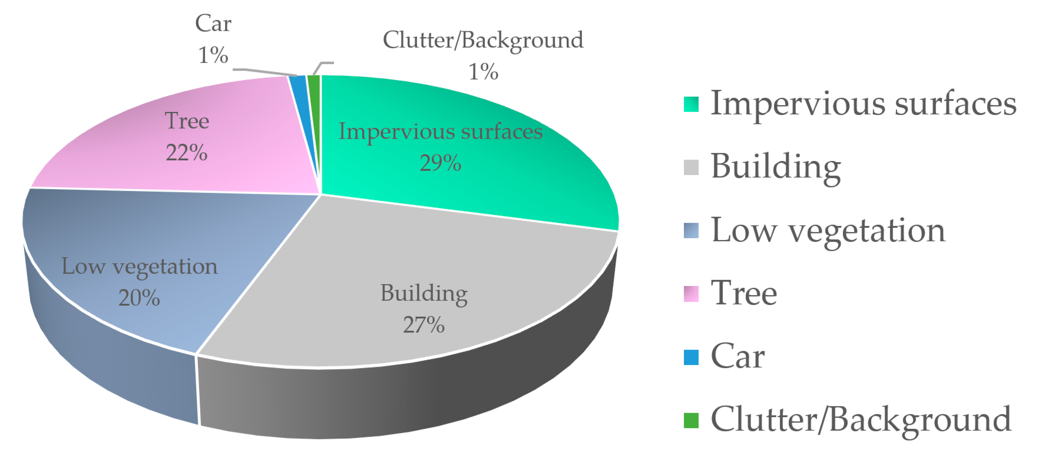
Figure 1. Some examples of multi-scale semantic segmentation and feature maps of remote sensing images. (a) The comparison between the ground truth and the segmentation effect of multi-scale objects in Fully Convolutional Network (FCN) is shown. (b) displays the visualization of deep feature map, in which the marked area is noise. (c) displays the visualization of shallow images.
Ijgi 10 00241 g001
Figure 2. The overall structure of the network. The encoder/decoder framework used in this network is mainly used to test the segmentation effect of the adaptive multi-scale module and the adaptive fuse module.
Ijgi 10 00241 g002
Figure 3. The left part (a) is the schematic diagram of spatial attention and channel attention. The right part (b) is the schematic diagram of a residual block in the residual network.
Ijgi 10 00241 g003
Figure 4. AMSM architecture diagram. The left part is the specific structure and various parameters of the three branches, and the right part is the topology image of an Adaptive Multi-Scale Module (AMSM).
Ijgi 10 00241 g004
Figure 5. The generation mechanism of spatial attention weight (SA weight) and channel attention weight (CA weight) [36] in Adaptive Multi-Scale Module. The number marked below the picture is the size of the convolution kernel.
Ijgi 10 00241 g005
Figure 6. AFM architecture diagram. The Adaptive Fuse Module consists of two parts. The left part (a) is the process of obtaining the weights of deep feature maps and shallow feature maps, aiming to achieve the filtering effect of deep features on shallow noise. The right part (b) is a schematic diagram of the operating mechanism of the Adaptive Fuse Module.
Ijgi 10 00241 g006
Figure 7. An input image sample and its ground truth in the ISPRS dataset. (a) This picture shows one of the input images of the ISPRS dataset. (b) The picture shows the ground truth corresponding to the picture in (a).
Ijgi 10 00241 g007
Figure 8. The proportion of pixels for each class in the training set.
Ijgi 10 00241 g008
Figure 9. On the ISPRS Vaihingen data set, six test results for the same baseline fusion of different modules. (a) Original input image; (b) ground truth; (c) baseline output image; (d) baseline and AMSM output image; (e) baseline and AFM output image; (f) baseline and fusion of AMSM and AFM. Vaihingen’s label includes six categories: impervious surface (white), building (blue), low vegetation (cyan), tree (green), car (yellow), and chaos/background (red).
Ijgi 10 00241 g009
Figure 10. The output image of our network compared with the classic network. Vaihingen’s label includes six categories: impervious surface (white), building (blue), low vegetation (cyan), tree (green), car (yellow), and chaos/background (red). (a) Input image. (b) U-net segmentation results. (c) Segmentation result of DeepLab-v3. (d) The segmentation result of SegNet. (e) We propose the segmentation result of AWNet. (f) Ground Truth.
Ijgi 10 00241 g010
Figure 11. The edge prediction output of our model and Pyramid Scene Parsing Network (PSPNet). Vaihingen’s label includes six categories: impervious surface (white), building (blue), low vegetation (cyan), tree (green), car (yellow), and chaos/background (red). (a) Input image. (b) Ground Truth. (c) A partial enlarged view of the PSPNet segmentation result. (d) A partial enlarged view of our proposed AWNet segmentation result.
Ijgi 10 00241 g011
Table 1. The pixel number of each class in the training set.
Class.Impervious SurfacesBuilding Low VegetationTreeCar Clutter/Background
Pixels Number 15,932,83714,647,182 11,008,08512,118,796 666,618 510,494
Table 2. Comparison between the baseline and the baseline with the corresponding model added.
IDExperimentOAAccuracy Improvement Ratio Compared with Baseline
1Baseline86.92%-
2Baseline + AMSM87.84%0.92%
3Baseline + AFM87.51%0.59%
4Baseline + AMSM + AFM88.35%1.43%
Table 3. The results of comparing our network with the landmark classic network.
ModelThe F1 Value of Each ClassMean F1 ScoreOA
Imp SurfBuildLow VegTreeCar
FCN88.6792.8376.3286.6774.2183.7486.51
U-net79.0579.9568.1070.5015.7262.6675.60
Deeplab-v366.1883.7464.5278.7836.3165.9173.86
SegNet80.2185.9770.3679.2426.7268.5079.87
DCCN86.4392.0779.3682.5466.4081.3685.31
AWNet(ours)90.3294.1180.2587.0582.2286.7988.35
Table 4. The results of a comparison between our network and an improved network based on the classic network.
ModelThe F1 Value of Each ClassMean F1 ScoreOA
Imp SurfBuildLow VegTreeCar
FCN-dCRF88.892.9976.5886.7871.7583.3886.65
SCNN88.2191.877.1787.2378.684.486.43
Dilated FCN90.1994.4977.6987.2476.7785.2887.7
CNN-FPL-----83.5887.83
PSPNet89.9294.3678.1987.1272.9784.5187.62
Deeplab v3+89.9294.2178.3187.0171.4384.1887.51
DANet89.3193.9978.2586.7471.2683.9187.44
AWNet(ours)90.3294.1180.2587.0582.2286.7988.35
Publisher’s Note: MDPI stays neutral with regard to jurisdictional claims in published maps and institutional affiliations.

