
Toward Improving Image Retrieval via Global Saliency Weighted Feature


1
College of Computer Science and Technology, Jilin University, Changchun 130012, China
2
Key Laboratory of Symbolic Computation and Knowledge Engineering of Ministry of Education, Jilin University, Changchun 130012, China
3
School of Mechanical Science and Engineering, Jilin University, Changchun 130025, China
*
Author to whom correspondence should be addressed.
ISPRS Int. J. Geo-Inf. 2021, 10(4), 249; https://0-doi-org.brum.beds.ac.uk/10.3390/ijgi10040249
Submission received: 6 February 2021
/
Revised: 4 April 2021
/
Accepted: 5 April 2021
/
Published: 8 April 2021
Abstract
:For full description of images’ semantic information, image retrieval tasks are increasingly using deep convolution features trained by neural networks. However, to form a compact feature representation, the obtained convolutional features must be further aggregated in image retrieval. The quality of aggregation affects retrieval performance. In order to obtain better image descriptors for image retrieval, we propose two modules in our method. The first module is named generalized regional maximum activation of convolutions (GR-MAC), which pays more attention to global information at multiple scales. The second module is called saliency joint weighting, which uses nonparametric saliency weighting and channel weighting to focus feature maps more on the salient region without discarding overall information. Finally, we fuse the two modules to obtain more representative image feature descriptors that not only consider the global information of the feature map but also highlight the salient region. We conducted experiments on multiple widely used retrieval data sets such as roxford5k to verify the effectiveness of our method. The experimental results prove that our method is more accurate than the state-of-the-art methods.
1. Introduction
Content-based image retrieval (CBIR) [1,2,3,4], with the advent of convolutional neural networks, has dramatically shaped queries in image retrieval in recent years. The volume of image databases is also increasing with the rapid development of computer and Internet technology. Developing quick and accurate methods to obtain the required images from large-scale image databases has become popular in research. Extracting the features of the image is the main aim of these methods. Then, the similarity of these features is measured and the retrieval results are finally obtained. Query extensions and other methods are quintessentially used as a supplement [5,6,7,8] to improve the accuracy of retrieval.
The research process of content-based image retrieval is mainly decomposed into two aspects: manual features and deep features. The initial image retrieval is mainly based on a few manual global features, such as color and texture [9,10,11], but because these manual global features are easily affected by occlusions, displacements, and lighting conditions, the retrieval performance is considerably reduced. To solve the problems affecting the manual global features, researchers have proposed manual local features that are not easily affected by scale changes and illumination [12,13]. The most representative method is the scale-invariant feature transform (SIFT) [12], which is invariant to image distortion, illumination changes, viewpoint changes, and scale scaling. Owing to the complexity and time-consuming compution of SIFT [12], speeded up robust features (SURF) [14] was proposed based on SIFT [12]. Bag-of-visual words (BoW) [15] was proposed to aggregate these local features into a global image representation. BoW [15] was inspired by text processing and regards the local features of the image as visual words so that the frequency of the local features in the image can be used to form a one-dimensional vector to describe the image. In addition to BoW [15], later aggregation technologies such as vector of locally aggregated descriptors (VLAD) [16], fisher kernels on visual vocabularies (FV) [17,18], and triangulation embedding [19] have achieved better results.
In the past few decades, manual features have been widely accepted in image retrieval, but the shortcomings of manual features cannot be ignored: they need to be designed by researchers in the professional field, and they are difficult to generalize to different application scenarios. Since 2012, image retrieval has fully entered an era based on deep features [20,21,22], which are widely used for three-dimensional convolution features obtained by deep convolutional neural networks in image retrieval tasks. When applying the features obtained through the convolutional layer to image retrieval, a problem arises: how to aggregate three-dimensional convolution features into one-dimensional convolution features for similarity measurement. The simplest sum-pooled convolutional (SPoC) [23] and maximum activation of convolutions (MAC) [24] are compressed into a one-dimensional feature vector by obtaining the maximum value and by summing the value of each feature map, but this causes a large amount of feature value information to be lost, so the regional maximum activation of convolutions (R-MAC) [25] was proposed to solve this problem. Using a multiscale method, the maximum value in each region is used to mine the information of each feature map, but the information contained in all feature points in each region is not considered. Cross-dimensional weighting (Crow) [26] is different from the previous methods using the idea of the attention mechanism to perform spatial weighting and channel weighting. The three-dimensional feature map obtained by weighting is then simply compressed to form a one-dimensional feature vector. Through the spatial weighting matrix and the channel weighting matrix, the weighted features can be more concentrated on the target region of the image. Unfortunately, this weighting cannot enhance the salient regions that are more conducive to image retrieval, such as building edges, architectural details, etc.
Given the above considerations, we introduce a novel deep convolution feature aggregation method. First, we propose a generalized R-MAC pooling method that can better represent the global information of the feature map. Second, we construct a method that uses spatial saliency-weighted feature maps to more accurately distinguish the target region from the background region. Then, we fuse the feature maps obtained by the two methods to form the ultimate descriptor. The main contributions of this paper can be summarized as follows:
- We introduce a novel feature pooling method, named generalized R-MAC, which can capture the information contained in all the feature points in each region of R-MAC [25] instead of only considering the maximum value of the feature points in each region.
- We present an approach for the aggregation of convolutional features, including nonparametric saliency weighting and pooling steps. It focuses more attention on the convolutional features of the salient region without losing the information of the entire building (target region).
- We conducted comprehensive experiments on several popular data sets, and the outcomes demonstrate that our method provides state-of-the-art results without any fine-tuning.
2. Related Work
2.1. Aggregation Methods
Since convolutional neural networks have been broadly adopted in the field of image retrieval, research hotspots have gradually concentrated on the fully connected layer instead of the convolutional layer of convolutional neural networks (CNNs). The features produced by the convolutional layer are more robust in image transformation, can more accurately express spatial information. Therefore, obtaining a more representative image descriptor becomes a key step to improving the accuracy of image retrieval.
In the early days, a multitude of classical encoding methods for hand-crafted features was used to generate image descriptors. SIFT [12] is a scale-invariant feature transformation that can detect key points in the image. BoW [15] uses clustered local image features as visual words and counts their frequency to construct image descriptors. VLAD, proposed by Jegou et al. [16], mainly trains a small codebook through the clustering method and encodes it according to the distance between the feature and the cluster center. Hao et al. proposed a multiscale fully convolutional (MFC) [27], which uses three different scales to extract features and fuses them to generate the ultimate descriptor.
In recent years, three-dimensional convolution features have been fused into more compact feature descriptors. Babenko et al. proposed SPoC [23] to calculate the average value of each feature map to obtain a compact feature descriptor. The calculation of this average value does not consider the importance of each feature value. The point with the larger feature value is more likely to be the target region. Razavian et al. proposed MAC [28] to calculate the maximum value of each feature map to obtain compact feature descriptors. Taking the maximum value of each feature map, although feature filtering is simple, it loses too much information contained in the feature map. R-MAC [25] performs sliding window sampling on deep convolutional features and takes the maximum value of each window aggregated into image feature descriptors. Compared with MAC, although R-MAC captures more information from each feature map in a multiscale manner, there are still problems with MAC when selecting the maximum value for each region obtained. Crow [26], proposed by Jimenez et al., cites the idea of the attention mechanism and performs spatial weighting and channel weighting on the convolution feature map to highlight the target region of the image aggregation method. The semantic-based aggregation (SBA) method was proposed by Xu et al. [29]. These aggregation methods improve the accuracy of retrieval to a certain extent, but they do not effectively use of the global information of the feature map and ignore focusing on the salient region of the feature map. Based on this, we propose global saliency-weighted deep convolution features, which makes the feature descriptors more representative of image information and achieves more accurate retrieval results. We conducted a comprehensive comparison test to prove that the algorithm we constructed exceeds various existing state-of-the-art algorithms.
2.2. Normalization and Whitening
Normalization is an overwhelmingly crucial step in image retrieval [30]. Normalization can convert data to a uniform range for comparison. L2 normalization [30] converts the data to a range between 0 and 1. The value range of the feature output by the convolutional neural network is usually extremely large. Accordingly, L2 normalization can be used to balance the size and value influence. The specific calculation is as follows:
where is a concrete vector and is a 2-norm value of this vector.
Power normalization [30] reduces the vector according to the power exponent. The specific calculation formula is as follows:
where is a configurable hyperparameter, ranging from 0 to 1. Additionally, is a concrete vector. To avoid transforming the sign of the value after power normalization, we use , called the sign function, which is defined as = 1 for and = −1 for .
Whitening has often been adopted as a postprocessing operation in image retrieval to whiten and reduce dimensions based on the work of Jegou and Chum [8]. When reducing dimensionality, we use whitening to prevent the interaction effect between raw data components and to reduce noise [7,31,32]. Here, we use whitening as a postprocessing step to improve our retrieval performance. The essence of whitening proposed by Mikolajczyk and Matas [32] is linear discriminant projections, which are divided into two parts.
In the first part, we obtain the covariance matrix of the intraclass images using Equation (3) and the covariance matrix of the interclass images (non-matched image pair) using Equation (4), where
where and denote two distinct images in the data set, and denote the feature descriptors after pooling of image, and () means that images and are associated with the same (different) class.
In the second part, we obtain the projection in the whitened space (the eigenvector of the covariance matrix ) and apply it in the descriptors of images:
where is the eigenvector of the specific matrix, is the mean pooling vector (a mean vector of the descriptors of all images in the test data set after pooling) to perform centering, and is the whitened result of . It is worth noting that Equation (5) does not take only the eigenvectors greater than a specific threshold for feature reduction.
2.3. Similarity Measurement Method
After obtaining the feature descriptors of the image, we need to measure the similarity between the feature descriptors of the query image and the feature descriptors of all the images in the test set. A commonly used method for computing the similarity of two vectors is based on the inverse of their Euclidean distance. The formula is as follows:
where and are two sample vectors, and and are the th components of vectors and , respectively. We denote by the Euclidean distance between and .
Cosine similarity is also used for similarity measurement, which uses the angle between two concrete vectors to calculate the cosine value to represent the similarity of two vectors. The closer the cosine value is to 1, the more similar the two vectors are. The closer the cosine value is to −1, the more dissimilar the two vectors are. The specific calculation formula is as follows:
where is the cosine similarity between and .
2.4. Query Expansion
Query expansion (QE) was first applied in text retrieval to improve effectiveness by extracting new keywords from top ranked results retrieved by an original query [5,6,7] to generate a new expanded query.
Inspired by this idea, where in image retrieval tasks, query expansion starts with a given query image, we retrieved top n ranked images, including the query image itself. Then, we calculated the average of these image features and generated a new query that is evaluated to re-rank [33] images. Query expansion expands the scope of image retrieval and is one of the postprocessing operations in image retrieval. Radenovic et al. [7] proposed α-weighted query expansion (αQE).
3. Proposed Method
3.1. Algorithm Background
Our algorithm calculates the descriptors of convolution features in two modules: generalized R-MAC (GR-MAC) and saliency joint weighting (SJW). They are introduced in detail in Section 3.2 and Section 3.3, respectively.
We obtain the ultimate feature descriptor by fusing the feature descriptors obtained by the two modules.
where comes from Section 3.2, comes from Section 3.3, and and are fusion factors with values ranging from 0 to 1.
GR-MAC inevitably weakens the influence of the salient region while obtaining more global information. Therefore, after integration of the SJW module, it is equivalent to assigning greater weight to the features of more important salient regions while obtaining global information. Such a fusion promotes the GR-MAC module of the data set with more obvious saliency regions. For more complex data sets with obvious saliency regions, there is a better improvement effect.
The algorithm provides five variables as input: is the three-dimensional feature map obtained by the last convolutional layer, is the number of channels selected, is the scale factor, and and are fusion factors. In this algorithm, for an input three-dimensional feature map, we obtain two different one-dimensional feature descriptors through Section 3.2 and Section 3.3, separately, and then normalize them separately. In the end, fusion is performed according to the values of and . After normalization and whitening, the final feature descriptor is obtained. The specific retrieval process is shown in Figure 1.
As shown in Figure 1, we briefly describe the specific retrieval process after using the global saliency weighting algorithm. We first used the pretrained network to extract the feature maps from the images in the data sets. Afterward, we used the generalized R-MAC and saliency joint-weighted deep convolutional feature described in detail in Section 3.2 and Section 3.3 to obtain one-dimensional descriptors for the feature maps, separately. GR-MAC considers the maximum value of each region while considering the information contained in other response values and aggregates the three-dimensional feature maps obtained by the pretraining network into one-dimensional descriptors with more global information. SJW introduces a saliency algorithm to weight the salient region to obtain a salient region that is more conducive to image retrieval, such as the feature descriptor of the edge of a building. Then, after the abovementioned one-dimensional descriptors obtain the normalization process separately, we merged them in a linear manner (such as Equation (10)). Finally, the fused feature descriptors were whitened to obtain the feature descriptors of for image retrieval to obtain the top K retrieval result, returning images that are most similar to the query image.
3.2. Generalized R-MAC
Motivation: in Section 2, we briefly introduced the original R-MAC [25] algorithm. First, the R-MAC [25] algorithm divides each feature map into multiple regions according to the scale, as shown in Figure 2. Then, it takes the maximum value for each region to aggregate and to obtain the final image feature descriptor.
As shown in Figure 2, we use to describe the size of scales. In R-MAC [25], A sliding window is used to extract square feature regions at different scales. When , the side length of the extracted square region is the minimum value of the height and width , namely . Assuming that the number of extracted regions is when , the side length of the region is and each scale will extract regions.
The specific operation details are as follows: taking the feature map of a channel as an example, the feature map is divided into regions and the result region is as follows:
where is the rth region of the th feature map.
The R regions of each channel are obtained by the above formula; the maximum value is retained in the R-MAC [25] algorithm for feature aggregation. However, using max pooling in each scale region of R-MAC [25] loses the information contained in other feature values in the region. A didactic example is provided to illustrate the phenomenon in Figure 3.
As shown in Figure 3, we assume that the black square is a channel-wise feature map after the convolution layer. Obviously, the blue and green squares are two different regions obtained by R-MAC [25]. As R-MAC [25] takes the maximum value for each region, the feature values obtained in the blue region and the green region are both 0.37, but it is apparent that the distributions of the feature values of the two regions are not the same. R-MAC [25] only obtains information at the maximum response of 0.37 in the region. Thus, R-MAC [25] ignores the amount of information contained in other feature values in the region. The feature values obtained by this part of the convolution are also part of the image representation.
Method: to solve this problem, we propose the idea of a generalized R-MAC.
As shown in Figure 4, we use the norm in each scale region of R-MAC [25] to integrate max pooling and average pooling. In this way, not only can we obtain the maximum value of the most representative feature obtained by convolution but also,through the average pooling of norm fusion, we can obtain the overall information contained in the region. Our proposed generalized R-MAC can obtain richer semantic information. Here, we designed an effective scheme to calculate the generalized R-MAC.
For the specific region division of each feature map, we follow the idea of R-MAC [25], as shown in Equation (11).
R-MAC [25] distills the maximum value in each region, but this loses the global feature information of the region. Hence, we use another strategy for calculating regional feature values, as shown in Equation (12). The specific method involves using the norm to fuse max pooling and sum pooling to obtain more representative regional features. The specific calculation formula is as follows:
where is the value calculated by the norm of the th region of the th feature map, where .
Compared with R-MAC selecting the largest feature value in each region as the representative of the region, the feature value calculated by Equation (12) is used as the representative of each region. In Equation (12), when the value of is the value of max pooling, and when, the value of is the value of average (avg) pooling. That is, the proportion of max pooling and avg pooling can be determined by adjusting the coefficient p. Accordingly, the finally obtained representative values of each region not only have the characteristics of max-pooling of the target region as the response value is larger but also have the characteristics of avg pooling, which does not lose the information contained in all the feature values in the region. In this way, each region within the scale can obtain a better expression of the feature value, and finally, a more representative image feature descriptor can be obtained.
According to the multiple regional feature values obtained by each channel, the regional feature values of the channel are summed to generate the ultimate feature vector descriptor , as follows:
where is the sum of the values obtained by all regions of the th channel and is the image immature descriptor using generalized R-MAC.
The resulting generalized R-MAC descriptor considers the overall information and maximum response in each region. It can more accurately describe the global information of convolution features.
3.3. Saliency Joint Weighting Method
Motivation: in Section 2, we briefly introduced the original cross-dimensional weighting (Crow) [26] algorithm. The Crow [26] algorithm performs spatial weighting and channel weighting on the convolution feature map. We find that the spatial matrix of Crow [26] only sums the feature maps of all channels and then normalizes it as a spatial weighting matrix. It is a simple operation to count the number of nonzero values in each channel and to assign greater weight to the channel, with more zero values corresponding to the feature. We think that this simple spatial weighting matrix and channel weighting matrix still has room for optimization. We intended to use the saliency algorithm to identify the salient region of the convolutional features and to apply greater weighting to the salient region to design a weighting matrix that is more beneficial for distinguishing the target region from the background noise region. Retaining the Crow [26] algorithm to pay more attention to the characteristics of the image target region also strengthens the salient regions that are more conducive to image retrieval, such as the edges of buildings.
Method: first, we use Figure 5 to introduce the general flow of our method.
As shown in Figure 5, we briefly describe the key steps of how to obtain the final saliency joint-weighted
(SJW) descriptor from the above equations. For an original image, we obtain the feature map through a pretrained neural network. The green squares in the image represent the feature map of each channel obtained by different convolution kernels. Then, through the variance-channel selection step, the feature maps corresponding to the first channels with the largest variance values are selected, and then, the spatial weighting matrix is obtained by Equation (18). The normalized spatial weighting matrix is obtained by Equation (19). In order to highlight the salient region we need, we first performed a saliency operation on the matrix from the spatial perspective to obtain the saliency weighting matrix obtained by Equation (20) and Equation (21). We then fused the matrix through Equation (22) to obtain the final spatial weighting matrix . Afterward, through Equation (23), the saliency joint weighted (SJW) feature maps were obtained by using the feature maps and the spatial weighting matrix , and then the preliminary descriptor was obtained by pooling. A series of blue cubes of different shades represent the saliency joint-weighted (SJW) feature maps. In order to make the final descriptor more representative, we weighed it from the perspective of the channel. Finally, raw descriptors obtained by sum pooling the saliency joint-weighted (SJW) feature maps and the channel weighting matrix obtained by Equation (17) were used as an element-wise product to obtain a one-dimensional saliency joint-weighted (SJW) descriptor. Among them, let and represent the sizes in the matrices , , , and to make the flowchart more intuitive, where the characters , , and represent the elements in the matrices, , and respectively; is an element in the channel weighting matrix .
First, for a specific image , we used the pretrained network without the fully connected layers to obtain the 3D activated tensor of dimensions, where denotes the number of feature maps output from the last convolution layer.
Then, similar to Crow [26], we also performed spatial weighting and channel weighting operations on the obtained convolution features. For our channel weighting matrix, unlike Crow [26], which only considers the number of nonzero quantities for each channel, we also considered the variance of each channel as a part of the consideration that affects the value of the channel weight matrix. The same as Crow [26], for each dimension of the feature map, the ratio of its sum value corresponding to the number of zero values was calculated in each feature map, and the obtained expression is as follows:
where is the ratio of the total spatial location in the th feature map to the zero value. We can judge the amount of information contained in a feature map by counting the number of nonzero amounts, which is used to improve features that are not often seen but are also meaningful.
Based on , we proposed adding a variance term to optimize the channel weight matrix, as shown in Equation (15). For the feature map of each channel to find its standard deviation, the obtained expression is as follows:
where is the average of and is the variance of the th channel.
Then, we calculated the proportions of and . After that, we summed them, and the resulting expression is as follows:
When aggregating deep convolution features, since we subsequently greatly strengthened the target channel and target region based on the variance and response value, the channel with less information may be ignored. However, such channels may also contain especially crucial information and channels with small variance can also suppress noise. Therefore, we needed to assign a larger weight to the feature channel with a large number of zeros and small variance. Finally, similar to Crow [26], the inversion operation was performed through the log function. The specific formula for obtaining the final channel weight vector using logarithmic transformation is as follows:
where is the channel weight and is an intensely small constant added to prevent the denominator from being zero.
Our spatial weighting matrix is different from Crow [26], which only sums and normalizes all the channel feature maps and then serves as the final spatial weighting matrix S. We firstly filtered the top k feature channels that are more conducive to distinguishing the target region from the background noise region through the variance to sum the initial weighting matrix S and then normalized the weighting matrixwhich is similar to Crow [26]. According to the obtained channel selection factor, we selected the channel with a large variance to superimpose the weighting matrix of the space because the channel with large variance is more conducive to the distinction between the target region and the background region. The specific calculation formula is as follows:
Let be the vector of channels’ variances. We denote as the top with the largest variance in . is the matrix of summing the feature values corresponding positions in all channels by .
Then, the obtained spatial weighting matrix is normalized and power-scaled to obtain the normalized weighting matrix .
We used the linear computational (LC) algorithm [34] to detect the saliency of the weighting matrix . First, we scaled the value of the obtained matrix M to between 0 and 255 to be applicable to the LC algorithm [34]. Then, we mapped the value of to the pixel space from 0 to 255 to calculate the subsequent saliency matrix. The mapping formula is as follows:
where is a weighting matrix that normalizes the value of to a range between 0 and 255.
Concerning the idea of the LC algorithm [34], we calculated the sum of the Euclidean distances between each point on the spatial weighting matrix and all other points as the response value of the point. Afterward, we obtained the spatial saliency weighting matrix. The specific calculation formula is as follows:
where is the feature value of the saliency weighting matrix at , .
Then, we fused the obtained saliency weighting matrix into the original weighting matrix with a certain scale factor, so that the final spatial weighting matrix assigns greater weight to the key region with a certain fusion factor, while the response information of the target region and the background noise region was retained in the original convolution feature. For the obtained spatial weighting matrix , we used a certain scale factor to fuse it into the spatial weighting matrix obtained by the previous channel selection so that the final weighting matrix can better highlight the target region of the feature map.
where is the fused factor and is the spatial weight matrix after saliency joint weighting.
Finally, we obtained the saliency joint-weighted (SJW) descriptor through the final spatial weighting matrix and the channel weighting matrix . We multiplied the obtained final spatial weighting matrix with the three-dimensional feature map obtained by convolution and then summed the feature maps of each channel to obtain a one-dimensional image descriptor .
where is the feature value obtained from the th feature map after spatial weighting and is the vector of all .
For the obtained one-dimensional descriptor , we used the channel weight vector obtained by the above Equation (17) for weight, so that the descriptor pays more attention to the important feature channels and forms the final spatial saliency-weighted descriptor .
where is the feature value obtained from the th feature map after the channel weighting and is the vector of all .
4. Experiments and Evaluation
In this section, to verify the rationality of our designed convolution feature aggregation scheme, we conducted many comparative experiments. First, we tested the effectiveness of the two modules separately, and then, we fused the two modules according to a certain scale factor. The experimental outcomes revealed that our proposed global saliency-weighted convolution feature achieves state-of-the-art performance.
4.1. Data Set
The retrieval data set was used to train and test the retrieval algorithm. In this section, we briefly introduce the data set used in the experiment.
- Oxford5k data set [33]: This data set is provided by Flickr and contains 11 landmarks in the Oxford data set and a total of 5063 images.
- Paris6k data set [35]: Paris6k is also provided by Flickr. There are 11 categories of Paris buildings, which includes 6412 images and 5 query regions altogether for each class.
- Holidays data set [36]: The Holidays data set consists of 500 groups of similar images; each group has a query image for a total of 1491 images.
- Revisited Oxford and Paris [37]: The Revised-Oxford (Roxford) and Revisited-Paris (Rparis) data sets consist of 4993 and 6322 images, respectively; each data set has 70 queries images. They re-examine the oxford5k and paris6k data sets by deleting comments and adding images. There are three difficulty levels of evaluation protocol: easy, medium, and hard.
4.2. Test Environment and Details
Our experiment was implemented on TITAN XP, and the graphics processing unit (GPU) memory was 11 G (the graphics card was composed of a GPU computing unit and video memory, etc. The video memory can be regarded as space, similar to memory). We used the PyTorch deep learning architecture to construct the VGG16 model [3], which was pretrained on ImageNet [38]. Hence, we did not need training. For the test, we used the VGG16 model to extract convolutional features maps from the conv5 layer, and the whole number of channels was 512. For our newly designed algorithms in testing, the first module (GR-RMAC) required 3 min 58 s and 2012 MB of video memory; the second module (SJW) required 19 min 13 s and 2138 MB of video memory; and the entire algorithm (GSW) required a total of 19 m 28 s and 2629 MB of video memory. The test cases were conducted on the oxford5k [33] and paris6k [35], Holidays [36], oxford105k, paris106k, Roxford, and Rparis data sets [37], which have 5063, 6412, 1491, 4993, and 6322 images, respectively. As for image size, we followed Crow [26], which maintains the original size of images as input. After parameter analysis, we set the best hyperparameters in all experiments: = 3, = 0.3, = 100, = 0.6, and = 0.4. In addition, we used the same network model, dimensions of image descriptor, and input size of image. The method used to calculate the similarity was the cosine similarity. For the general evaluation standard, we used mean average precision () [33] and precision.
The average precision () measures the quality of the learned model in each category. measures the quality of the learned model in all categories. After the was obtained, the average value was taken. The range of values was between 0 and 1. The specific , calculation formula is as follows:
where is the resulting images returned that are relevant to the query image, is the volume of returned images during retrieval, and is the volume of images in the test data set that is relevant to the query image.
where is the quantity of the query images in a data set.
Precision means that, given a specific number of returned images in image retrieval, the ratio of the number of correct images to the number of returned images denotes the accuracy of returning an image in the retrieval, while denotes the accuracy of returning five images in the retrieval.
4.3. Testing the Two Modules Separately
Next, we conducted various comparative experiments on the two proposed aggregation modules, which generally reduce the influence of noise. Thus, we use whitening without reducing dimensions to increase precision. To further compare our approach with R-MAC [25] and Crow [26], we evaluated the performance of the generalized R-MAC pooling module and the saliency joint-weighted deep convolutional feature module on the Oxford5k, Paris6k, Holidays, Roxford5k, and Rparis6k data sets with VGG16.
Table 1 illustrates the outcomes of the R-MAC [25] and generalized R-MAC feature descriptors. By observing this table, we find that, when we tested on VGG16, the of Paris6k, Oxford5k, and Holidays using Generalized R-MAC (GR-MAC) was 83.63%, 70.35%, and 89.58%, respectively. Simultaneously, the best retrieval outcomes were obtained.
Table 2 shows the results of the R-MAC [25] and the GR-MAC feature descriptors. By observing this table, we conclude that, when we test on VGG16, the for Roxford5k-Easy and Rparis6K-Easy achieved using GR-MAC was 63.33% and 80.15%, respectively; the P@1 and P@5 of Roxford-Easy and Rparis-Easy using GR-MAC was 85.29% and 78.24%, and 95.71% and 93.71%, respectively; and the of Roxford-Medium and Rparis-Medium using GR-MAC was 42.26% and 63.86%, respectively. The P@1 and P@5 of Roxford-Medium and Rparis-Medium using GR-MAC were 84.29%, 70.19%, 95.71%, and 96.29%, respectively, and the best retrieval results were obtained.
After a series of comparative experiments using R-MAC [25] and our improved generalized R-MAC (GR-MAC) on five data sets, it is clear that our algorithm is better than R-MAC [25] by analyzing the experimental data in Table 1 and Table 2, that is, the effectiveness of our method was verified. Compared with R-MAC taking the maximum value for each divided region, we took the maximum value while considering the influence of other response values in the region so that the image feature descriptor we use obtains better results during retrieval. By comparing the test results, we find that, for the more difficult Oxford5k, Roxford, and Rparis data sets, our improved generalized R-MAC (GR-MAC) is more accurate and that, for the simple Paris6k and Holidays data sets, our method also provides a small improvement.
Table 3 indicates the outcomes of the cross-dimensional weighting (Crow) [26] and saliency joint weighting (SJW) methods. From this table, we learn that, when we test on VGG16, the of the Paris6k, Oxford5k, and Holidays data sets using saliency joint weighting (SJW) is 79.41%, 69.62%, and 89.74%, respectively, which are the best retrieval results.
Table 4 indicates the outcomes of the cross-dimensional weighting (Crow) [26] and the saliency joint-weighted feature descriptors. From this table, we learn that, when we test on VGG16, the of Roxford5k-Easy and Rparis6K-Esay using GR-MAC is 63.09% and 78.68%, respectively; the P@1 and P@5 of Roxford-Easy and Rparis-Easy using GR-MAC are 88.24% and 75.00%, and 97.14% and 93.71%, respectively. The of Roxford-Medium and Rparis-Medium using GR-MAC is 47.36% and 60.90%, respectively; the P@1 and P@5 of Roxford-Medium and Rparis-Medium using GR-MAC are 87.14% and 72.57%, and 97.14% and 96.00%, respectively, and the best retrieval results are obtained.
In addition, given the adequacy of experiments, we conducted a comparative test of Crow [26] and our improved saliency joint weighting (SJW) method on five data sets. By analyzing the experimental data in Table 3 and Table 4, we show that our algorithm is better than Crow [26] on the five data sets, which verifies the effectiveness of our method. Compared with the feature descriptor obtained by Crow’s [26] spatial weighting and channel weighting, the saliency weighting matrix obtained by the saliency detection algorithm is more conducive to distinguishing the salient region, and the image feature descriptor obtained by the improved channel weighting matrix achieves better results in retrieval.
We visualized the heat map for improved saliency weighting (SW) and saliency joint weighting (SJW) and found that the saliency weighting matrix pays more attention to a slice of salient regions that can distinguish different buildings, such as the edge information of the overall shape of the building or the detailed information of the window grille shape. However, these salient regions are the key regions in general image retrieval (such as building data sets). Obviously, as shown in the visualization in Figure 5, column b, the key region is brighter than the others. The ability to represent feature maps has a strong influence on the accuracy of image retrieval. Therefore, in order to improve the expressive ability of the feature map, we explored it from two perspectives to improve the feature map from the original convolutional layer to improve its representativeness. From a spatial perspective, we used the saliency weighting matrix to highlight the feature values of the salient region. At the same time, the feature maps of the convolutional layer were fused proportionally. As shown in column c of Figure 5, the above saliency joint weighting scheme can make the improved feature map pay more attention to the salient region without losing the overall building information obtained by the deep neural network. From a channel perspective, we used nonzero quantities and channel variance to measure the importance of different channels and used channel weighting to obtain the final saliency joint-weighted (SJW) descriptor .
As shown in Figure 6, we randomly selected images and obtained their origin feature maps, saliency-weighted (SW) maps, and saliency joint-weighted (SJW) heat maps. Through the comparison of heat maps, we found that our saliency joint weighting method can make the target region more prominent without ignoring the information of other regions. (a) We randomly selected three original images from the Oxford5k data set [33]. (b) The SW map means a saliency-weighted map for which drawing data were from the result calculated by Equations (16) and (17). After visualization, we found that the saliency-weighted map can focus on the target region of the image. (c) SJW map means the saliency joint-weighted map. The obtained saliency-weighted map was fused with the original features to a certain extent using a scale factor to obtain the final saliency joint-weighted map, as shown in Equation (22). From the analysis of the above results, it can be seen that our saliency joint-weighted (SJW) feature focuses on the key region of retrieval, without losing other parts of information.
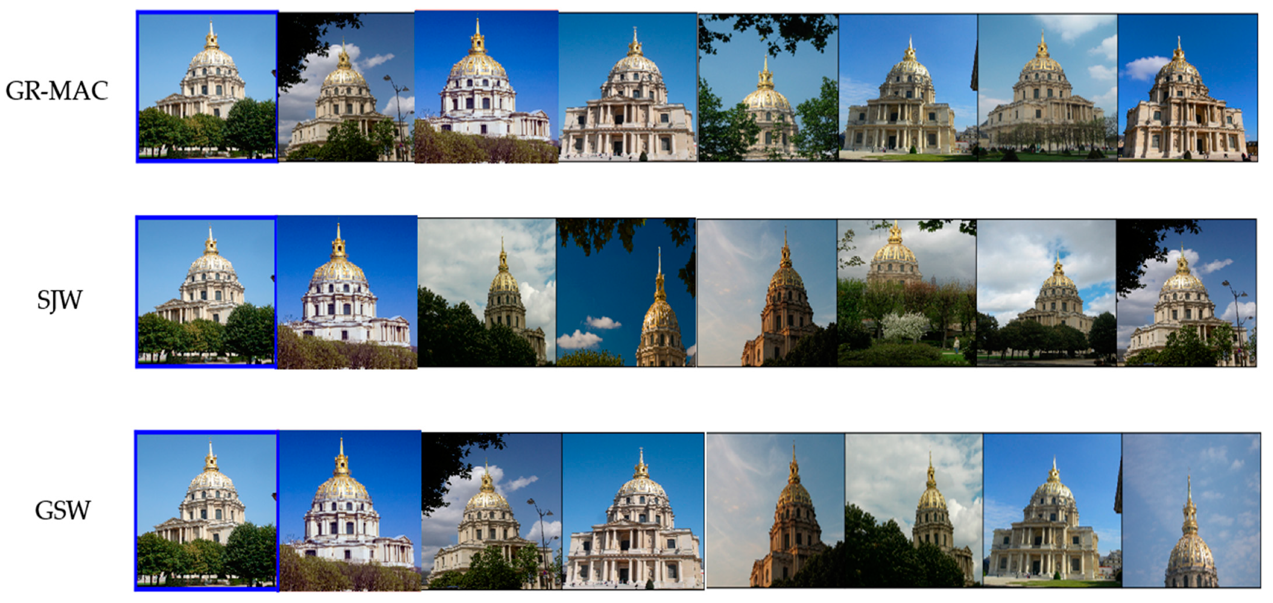
The results of the experimental application of this retrieval result analysis procedure are provided to illustrate the proposed algorithm. As shown in Figure 7, the query image (the image in the blue box) corresponds to the return images of the module’s retrieval results. The first row is the retrieval results of GR-MAC, the second row is the retrieval results of SJW, and the third row is the retrieval results of GSW. Comparing the two rows of images, as discussed, the differences are due to the two modules focusing on differences. GR-MAC pays more attention to global information, and the first line returns a more similar overall building. SJW pays more attention to salient local details, and the second row can return the partial details of the building that are partially obscured (such as the dome-shaped top). GSW can return both images with global information and images with more attention to salient details.
4.4. Feature Aggregation Method Comparison
We conducted retrieval experiments on the global saliency-weighted (GSW) descriptor. Query expansion can further enhance the performance of image retrieval. In this section, we use our method to calculate feature descriptors. Then, we verify the benefit of query expansion on the Oxford5k, Paris6k, and Holidays data sets.
Table 5 illustrates the outcomes of different feature descriptors before and after query expansion. By observing this table, we find that, when we tested on VGG16, the SJW module obtained more discriminative global features for data sets with more saliency regions. For example, oxford5k had a significant effect on improvement. The accuracy rate of GR-MAC in Table 5 is 70.35%, and the effect after integrating the SJW module can reach 72.90%, since there are many images in the Paris6k data set that do not have obvious saliency regions. Our GR-MAC algorithm, which is more conducive to obtaining global information, produced better results than the GSW algorithm, which incorporates saliency weighting. The of the Paris6k, Oxford5k, and Holidays data sets using GSW (ours) + QE was 89.55%, 79.87%, and 91.51%, respectively. Obviously, the best retrieval results were obtained. By observing Table 6, we drew the inference that the results for the features probably increase when we apply the operation of query expansion on diverse data sets.
From the experimental results, we conclude that the previous post-QE operations used to improve retrieval accuracy are also very applicable to our proposed algorithm. Regardless of the feature descriptor obtained from the GR-MAC or SJW module, or the feature descriptor obtained from the fusion of the two modules, the QE operation in the subsequent retrieval process greatly improves our retrieval effect.
To prove the effectiveness and superiority of our proposed global saliency-weighted convolution feature algorithm, we compared the experimental results with the latest feature aggregation algorithms. We not only conducted experiments using the original image representation but also compared the experimental results through query expansion. The outcomes are displayed in Table 6 and Table 7.
Table 6 reveals that only by using our method can we obtain the best results and that better results can be obtained through query expansion. The above experiments fully validated the utility and excellence of our algorithm. In Table 6, because there is no experiment under this condition in the literature of the corresponding methods, we replaced the missing value with a small horizontal line.
Table 7 indicates that only by using our method can we obtain the best results and that better results can be obtained through query expansion. Our algorithm not only provided promising results on the classic data set but also provided greatly improved results on the new building data set revised in 2018, which further proves the generalization ability of the algorithm.
The extensive results in Table 6 and Table 7 show that the two proposed modules have mutual promotion effects. The feature descriptors obtained by fusing the two modules achieve the best accuracy for subsequent retrieval operations. Compared with the previous method, we find that, on the five data sets, the retrieval effect provided by our method is significantly improved. A higher accuracy rate can be achieved after the QE operation.
4.5. Discussion
From the experiments above, key findings emerge:
1. The proposed generalized R-MAC (GR-RMAC) algorithm produces a better retrieval effect than the regional maximum activation of convolutions (R-MAC) [25] algorithm by capturing more effective information in multiple regions of R-MAC [25].
2. Our proposed saliency joint weighting (SJW) algorithm produces a more excellent spatial weighting matrix and channel weighting matrix through saliency detection. Compared with the previous cross-dimensional weighting (Crow) [26] obtained by spatial weighting and channel weighting, our weighting method effectively improves the retrieval performance.
3. We fused the feature descriptors obtained by GR-RMAC and SJW as the final retrieval feature and found that the two proposed modules have a mutual promotion effect. This fusion achieved the best retrieval effect. Comparing it with the previous algorithm, our method provided significantly improved results on multiple data sets.
Two limitations of these two aggregation modules are that it may be suitable for instance retrieval and not for other types of image retrieval that require higher saliency precision. Simultaneously, the calculated amount of the two modules is not low, so we will further optimize this in the future to reduce the computational burden of retrieval and study a more versatile aggregation method.
4.6. Parameter Analysis
In this section, we test the primary parameters of our algorithm on the oxford5k data set [33]. We used the same evaluation criterion, mAP, on the previous feature pooling methods (SPoC [23], MAC [24], R-MAC [25], Crow [26], etc.) to measure the accuracy of retrieval. We tested the best parameters on oxford5k and applied them to the other four data sets.
In the calculation process of global saliency-weighted aggregated convolution features, we used a total of five adjustable parameters: the scale of the R-MAC [25] division region, the number of channels selected by the three-dimensional feature map, the proportion of the fusion saliency weighting matrix factor, and the scale factors and that combine the generalized R-MAC module and the saliency joint-weighted deep convolutional feature module. By adjusting these parameters for the calculation of global aggregated saliency-weighted convolutional features, we selected the best parameters to obtain the final feature descriptor to enable the descriptor obtained by the generalized R-MAC module and the saliency joint-weighted deep convolutional feature module for fusion. We first performed normalization for them and then performed normalization after fusion to obtain the final feature descriptor to facilitate subsequent whitening operations.
Firstly, we tested the value of the scale parameter, which determines the number of regions divided in the GR-MAC algorithm. When the value of is too small, it does not reflect the advantage of obtaining more information on multiple scales. When the value of is too large, there will be large amounts of repeated information collected and this information may be the background region and may not necessarily all contribute to the image. Thus, a larger is not necessarily better.
We aimed to select the optimal so that the GR-MAC algorithm could obtain the optimal number of regions .
Table 8 detects the results of parameter . To obtain the best feature descriptors, we tested the value of between 1 and 4. The was the highest at , and the maximum value is bolded in Table 8. We chose to obtain the final generalized R-MAC feature descriptor.
Then, we tested the parameter described in Section 3.2. The parameter represents the number of feature maps selected in the saliency joint-weighted deep convolutional feature module. We sampled uniformly and then experimented on the Oxford5k data set. The network used was a pretrained VGG16. The result is shown in Table 9.
We aimed to choose a moderate . The value of n should be neither too small, which would lose too much feature channel information, nor too large, which would make our selection process an invalid operation. We aimed to choose the most appropriate so that the chosen feature channel would contain enough information after the summation. At the same time, due to the large variance in these channels, it was more conducive to distinguish the target region from the background region.
From Table 9, we can infer that the obtains the maximum value at = 30%. The maximum value is bolded. We chose = 30% to obtained the final saliency joint-weighted feature descriptor.
We tested the parameterdescribed in Section 3.2. The parameter represents the scale factor of the spatial weighting matrix-aggregated saliency weighting matrix in the saliency joint-weighted deep convolutional feature module. If is too large, it may focus too much on the target region and ignore the background regions containing a certain amount of information. If is too small, it may not focus on the desired target information. We used the VGG16 network pretrained on ImageNet in the experiments to experiment with ranging from 1 to 500. The results are listed in Table 10.
From Table 10, we conclude that obtains a maximum value at = 100. The maximum value is bolded. We chose = 100 to obtain the final saliency joint-weighted feature descriptor.
Finally, the obtained generalized R-MAC feature descriptor and saliency joint-weighted feature descriptor were tested for the fusion scale factorsand . We used the VGG16 network pretrained on ImageNet to test the Oxford5k data set, and the results are shown in Table 11.
We used the fusion factors and to fuse the image feature descriptors obtained by the GR-MAC algorithm and SJW algorithm to obtain the final GSW feature for retrieval. The feature descriptors obtained by GR-MAC focus more attention on the global information of feature maps on multi-scales. Under the influence of the saliency algorithm, the feature descriptor obtained by SJW focuses on the saliency region that is most conducive to image retrieval while focusing on the target region and ignoring the background region. The two descriptors have their advantages; consequently, we hoped to find the most effective fusion ratio and to obtain the feature descriptor with the best retrieval effect.
From Table 11, the results demonstrated that obtains the maximum value at = 0.6 and = 0.4. The maximum value is bolded. We chose = 0.6 and = 0.4 to obtain the final global saliency weighting feature descriptor.
From Table 12, we used Alexnet to perform module ablation experiments on the oxford5k and paris6k data sets, separately, to illustrate that our proposed method is still applicable in other models. Together, the findings confirmed that the feature maps obtained by different pretrained models have a certain impact on the retrieval effect, but for the feature maps obtained under the same network, the feature descriptors obtained by our method are better than the previous algorithm.
5. Conclusions
In this paper, we constructed two effective aggregation and improvement methods for deep convolution features and then merged them. The final retrieval accuracy reached state-of-the-art levels. We improved the classic regional maximum activation of the convolutions (R-MAC) [25] method and proposed a generalized R-MAC (GR-MAC) aggregation method, which allows the descriptor to obtain richer global information and is not limited to a single maximum value. Not only does the saliency joint weighting (SJW) module give the function of the convolutional layer feature an intuitive impression but also the obtained SJW feature pays more attention to the salient region of the image without losing the overall information of the building, improving the retrieval performance to better than that provided by current methods. After fusing the two proposed improved modules, they produced better retrieval performance on multiple building data sets.
Collectively, regardless of the proposed improved module, network training is not required. This nonparametric and easy-to-implement module allows the two proposed aggregation modules to be easily embedded in any other deep learning tasks. Future research should consider the potential effects of these two aggregation modules on more deep learning tasks, such as target detection and few-shot learning.
Author Contributions
Conceptualization, Hongwei Zhao; data curation, Jiaxin Wu; investigation, Hongwei Zhao; methodology, Hongwei Zhao and Danyang Zhang; project administration, Pingping Liu; resources, Hongwei Zhao and Pingping Liu; software, Jiaxin Wu; supervision, Pingping Liu; validation, Jiaxin Wu and Danyang Zhang; writing—original draft, Danyang Zhang; writing—review and editing, Jiaxin Wu and Pingping Liu. All authors have read and agreed to the published version of the manuscript.
Funding
This research was funded by the Nature Science Foundation of China, under grant 61841602; the Fundamental Research Funds of Central Universities, JLU, General Financial Grant from China Postdoctoral Science Foundation, under grants 2015M571363 and 2015M570272; the Provincial Science and Technology Innovation Special Fund Project of Jilin Province, under grant 20190302026GX; the Natural Science Foundation of Jilin Province, grant number 20200201037JC; the Jilin Province Development and Reform Commission Industrial Technology Research and Development Project, under grant 2019C054–4; the State Key Laboratory of Applied Optics Open Fund Project, under grant 20173660; Jilin Provincial Natural Science Foundation No. 20200201283JC; Foundation of Jilin Educational Committee No. JJKH20200994KJ; the Higher Education Research Project of Jilin Association for Higher Education, grant number JGJX2018D10; and the Fundamental Research Funds for the Central Universities for JLU.
Institutional Review Board Statement
Not applicable.
Informed Consent Statement
Not applicable.
Data Availability Statement
Data and the optimal network mode for this research work are stored in Github: https://github.com/wujx990/feizai_upload, accessed on 6 April 2021.
Conflicts of Interest
The authors declare no conflict of interest.
References
- Alzu’bi, A.; Amira, A.; Ramzan, N. Content-Based Image Retrieval with Compact Deep Convolutional Features. Neurocomputing 2017, 249, 95–105. [Google Scholar] [CrossRef] [Green Version]
- Smeulders, A.W.M.; Worring, M.; Santini, S.; Gupta, A.; Jain, R. Content-based image retrieval at the end of the early. IEEE Trans. Pattern Anal. Mach. Intell. 2001, 22, 1349–1380. [Google Scholar] [CrossRef]
- Yue-Hei Ng, J.; Yang, F.; Davis, L.S. Exploiting local features from deep networks for image retrieval. In Proceedings of 2015 Proceedings of the IEEE Conference on Computer Vision and Pattern Recognition Workshops, New York, NY, USA, 7–12 June 2015; pp. 53–61. [Google Scholar]
- Zheng, L.; Yang, Y.; Tian, Q. SIFT Meets CNN: A Decade Survey of Instance Retrieval. IEEE Trans. Pattern Anal. Mach. Intell. 2018, 40, 1224–1244. [Google Scholar] [CrossRef] [PubMed] [Green Version]
- Chum, O.; Philbin, J.; Sivic, J.; Isard, M.; Zisserman, A. Total recall: Automatic query expansion with a generative feature model for object retrieval. In Proceedings of the 2007 IEEE 11th International Conference on Computer Vision, Rio de Janeiro, Brazil, 14–21 October 2007; pp. 1–8. [Google Scholar]
- Chum, O.; Mikulik, A.; Perdoch, M.; Matas, J. Total recall II: Query expansion revisited. In Proceedings of the 2011 IEEE Conference on Computer Vision and Pattern Recognition, Colorado Springs, CO, USA, 20–25 June 2011; pp. 889–896. [Google Scholar]
- Filip, R.; Giorgos, T.; Ondrej, C. Fine-tuning CNN Image Retrieval with No Human Annotation. IEEE Trans. Pattern Anal. Mach. Intell. 2017, 41, 1655–1668. [Google Scholar]
- Jégou, H.; Chum, O. Negative evidences and co-occurrences in image retrieval: The benefit of PCA and whitening. In Proceedings of the 2012 European Conference on Computer Vision, Florence, Italy, 7–13 October 2012; pp. 774–787. [Google Scholar]
- Oliva, A.; Torralba, A. Modeling the Shape of the Scene: A Holistic Representation of the Spatial Envelope. Int. J. Comput. Vision 2001, 42, 145–175. [Google Scholar] [CrossRef]
- Oliva, A.; Torralba, A. Scene-centered description from spatial envelope properties. In Proceedings of the 2002 International Workshop on Biologically Motivated Computer Vision, Tübingen, Germany, 22–24 November 2002; pp. 263–272. [Google Scholar]
- Jain, A.K.; Vailaya, A. Image retrieval using color and shape. Pattern Recognit. 1996, 29, 1233–1244. [Google Scholar] [CrossRef]
- Lowe, D.G. Distinctive Image Features from Scale-Invariant Keypoints. Int. J. Comput. Vision 2004, 60, 91–110. [Google Scholar] [CrossRef]
- Tolias, G.; Furon, T.; Jégou, H. Orientation covariant aggregation of local descriptors with embeddings. In Proceedings of the 2014 European Conference on Computer Vision, Zurich, Switzerland, 6–12 September 2014; pp. 382–397. [Google Scholar]
- Bay, H.; Tuytelaars, T.; Van Gool, L. Surf: Speeded up robust features. In Proceedings of the 2006 European Conference on Computer Vision, Graz, Austria, 7–13 May 2006; pp. 404–417. [Google Scholar]
- Sivic, J.; Zisserman, A. Video Google: A text retrieval approach to object matching in videos. In Proceedings of the 2003 Computer Vision, IEEE International Conference on, Nice, France, 13–16 October 2003; p. 1470. [Google Scholar]
- Jégou, H.; Perronnin, F.; Douze, M.; Sánchez, J.; Pérez, P.; Schmid, C. Aggregating local image descriptors into compact codes. IEEE Trans. Pattern Anal. Mach. Intell. 2011, 34, 1704–1716. [Google Scholar] [CrossRef] [PubMed] [Green Version]
- Perronnin, F.; Dance, C. Fisher kernels on visual vocabularies for image categorization. In Proceedings of the 2007 IEEE Conference on Computer Vision and Pattern Recognition, Minneapolis, MN, USA, 17–22 June 2007; pp. 1–8. [Google Scholar]
- Perronnin, F.; Sánchez, J.; Mensink, T. Improving the fisher kernel for large-scale image classification. In Proceedings of the 2010 European Conference on Computer Vision, Heraklion, Crete, Greece, 5–11 September 2010; pp. 143–156. [Google Scholar]
- Jégou, H.; Zisserman, A. Triangulation embedding and democratic aggregation for image search. In Proceedings of the 2014 IEEE Conference on Computer Vision and Pattern Recognition, San Francisco, CA, USA, 23–28 June 2014; pp. 3310–3317. [Google Scholar]
- Cimpoi, M.; Maji, S.; Vedaldi, A. Deep filter banks for texture recognition and segmentation. In Proceedings of the 2015 IEEE Conference on Computer Vision and Pattern Recognition, Boston, MA, USA, 7–12 June 2015; pp. 3828–3836. [Google Scholar]
- Ghodrati, A.; Diba, A.; Pedersoli, M.; Tuytelaars, T.; Van Gool, L. DeepProposals: Hunting Objects and Actions by Cascading Deep Convolutional Layers. Int. J. Comput. Vision 2017, 124, 115–131. [Google Scholar] [CrossRef] [Green Version]
- Babenko, A.; Slesarev, A.; Chigorin, A.; Lempitsky, V. Neural codes for image retrieval. Proceedings of 2014 European Conference on Computer Vision, Zurich, Switzerland, 6–12 September 2014; pp. 584–599. [Google Scholar]
- Babenko, A.; Lempitsky, V. Aggregating local deep features for image retrieval. In Proceedings of the 2015 IEEE International Conference on Computer Vision, NW Washington, DC, USA, 7–13 December 2015; pp. 1269–1277. [Google Scholar]
- Razavian, A.S.; Sullivan, J.; Carlsson, S.; Maki, A. Visual instance retrieval with deep convolutional networks. Trans. Media Technol. Appl. 2016, 4, 251–258. [Google Scholar] [CrossRef] [Green Version]
- Tolias, G.; Sicre, R.; Jégou, H. Particular object retrieval with integral max-pooling of CNN activations. arXiv 2015, arXiv:1511.05879. [Google Scholar]
- Kalantidis, Y.; Mellina, C.; Osindero, S. Cross-dimensional weighting for aggregated deep convolutional features. In Proceedings of the 2016 European Conference on Computer Vision, Amsterdam, The Netherlands, 11–14 October 2016; pp. 685–701. [Google Scholar]
- Hao, J.; Wang, W.; Dong, J.; Tan, T. MFC: A multi-scale fully convolutional approach for visual instance retrieval. In Proceedings of the 2017 IEEE International Conference on Multimedia & Expo Workshops (ICMEW), San Diego, CA, USA, 23–27 July 2018; pp. 513–518. [Google Scholar]
- Sharif Razavian, A.; Azizpour, H.; Sullivan, J.; Carlsson, S. CNN features off-the-shelf: An astounding baseline for recognition. In Proceedings of the 2014 IEEE Conference on Computer Vision and Pattern Recognition Workshops, Columbus, OH, USA, 24–27 June 2014; pp. 806–813. [Google Scholar]
- Xu, J.; Wang, C.; Qi, C.; Shi, C.; Xiao, B. Unsupervised Semantic-Based Aggregation of Deep Convolutional Features. IEEE Trans. Image Process. 2019, 28, 601–611. [Google Scholar] [CrossRef] [PubMed]
- Szegedy, C.; Liu, W.; Jia, Y.; Sermanet, P.; Reed, S.; Anguelov, D.; Erhan, D.; Vanhoucke, V.; Rabinovich, A. Going deeper with convolutions. In Proceedings of the 2015 IEEE Conference on Computer Vision and Pattern Recognition, Boston, MA, USA, 7–12 June 2015; pp. 1–9. [Google Scholar]
- Gordo, A.; Larlus, D. Beyond instance-level image retrieval: Leveraging captions to learn a global visual representation for semantic retrieval. In Proceedings of the 2017 IEEE Conference on Computer Vision and Pattern Recognition, San Francisco, CA, USA, 21–26 July 2017; pp. 6589–6598. [Google Scholar]
- Mikolajczyk, K.; Matas, J. Improving descriptors for fast tree matching by optimal linear projection. In Proceedings of the 2007 IEEE 11th International Conference on Computer Vision, Rio de Janeiro, Brazil, 14–21 October 2007; pp. 1–8. [Google Scholar]
- Philbin, J.; Chum, O.; Isard, M.; Sivic, J.; Zisserman, A. Object retrieval with large vocabularies and fast spatial matching. In Proceedings of the 2007 IEEE Conference on Computer Vision and Pattern Recognition, Minneapolis, MN, USA, 17–22 June 2007; pp. 1–8. [Google Scholar]
- Zhai, Y.; Shah, M. Visual attention detection in video sequences using spatiotemporal cues. In Proceedings of the 14th ACM International Conference on Multimedia, Santa Barbara, CA, USA, 23–27 October 2006; pp. 815–824. [Google Scholar]
- Philbin, J.; Chum, O.; Isard, M.; Sivic, J.; Zisserman, A. Lost in quantization: Improving particular object retrieval in large scale image databases. In Proceedings of the 2008 IEEE Conference on Computer Vision and Pattern Recognition, Anchorage, AK, USA, 23–28 June 2008; pp. 1–8. [Google Scholar]
- Jegou, H.; Douze, M.; Schmid, C. Hamming embedding and weak geometric consistency for large scale image search. In Proceedings of the 2008 European Conference on Computer Vision, Marseille, France, 12–18 October 2008; pp. 304–317. [Google Scholar]
- Radenović, F.; Iscen, A.; Tolias, G.; Avrithis, Y.; Chum, O. Revisiting oxford and paris: Large-scale image retrieval benchmarking. In Proceedings of the 2018 IEEE Conference on Computer Vision and Pattern Recognition, Salt Lake City, UT, USA, 18–22 June 2018; pp. 5706–5715. [Google Scholar]
- Deng, J.; Dong, W.; Socher, R.; Li, L.-J.; Li, K.; Fei-Fei, L. Imagenet: A large-scale hierarchical image database. In Proceedings of the 2009 IEEE Conference on Computer Vision and Pattern Recognition, Miami, FL, USA, 20–25 June 2009; pp. 248–255. [Google Scholar]
- Liu, P.; Gou, G.; Guo, H.; Zhang, D.; Zhou, Q. Fusing Feature Distribution Entropy with R-MAC Features in Image Retrieval. Entropy 2019, 21, 1037. [Google Scholar] [CrossRef] [Green Version]
- Mohedano, E.; McGuinness, K.; O’Connor, N.E.; Salvador, A.; Marques, F.; Giró-i-Nieto, X. Bags of local convolutional features for scalable instance search. In Proceedings of the 2016 ACM on International Conference on Multimedia Retrieval, Vancouver, BC, Canada, 6–9 June 2016; pp. 327–331. [Google Scholar]
- Maaten, L.V.D. Accelerating t-SNE using tree-based algorithms. J. Mach. Learn. Res. 2014, 15, 3221–3245. [Google Scholar]
Figure 1.
Global saliency-weighted deep convolution features for image retrieval. CNN, convolutional neural network; R-MAC, regional maximum activation of convolutions; GSW, global saliency weighted.
Figure 1.
Global saliency-weighted deep convolution features for image retrieval. CNN, convolutional neural network; R-MAC, regional maximum activation of convolutions; GSW, global saliency weighted.

Figure 2.
Regional maximum activation of convolution (R-MAC) [25]. The squares of different colors represent the different divided regions, and the dots of different colors represent the center of each region.
Figure 2.
Regional maximum activation of convolution (R-MAC) [25]. The squares of different colors represent the different divided regions, and the dots of different colors represent the center of each region.

Figure 3.
The blue and green squares are two regions divided by R-MAC [25] in a channel-wise feature map. The distribution differs in these two regions.
Figure 3.
The blue and green squares are two regions divided by R-MAC [25] in a channel-wise feature map. The distribution differs in these two regions.

Figure 4.
Generalized R-MAC. The squares with different green depths represent the feature maps of each channel obtained by an image through different convolution kernels, and the regions are divided. A series of green circles in the figure indicate that each region of a channel-wise feature map passes through the feature values calculated by the norm. In the same way, the blue circle, the green circle, etc. are a series of feature values obtained in each region of other channels. The GR-MAC descriptor means the feature vector produced by the generalized R-MAC, as shown in Equation (13).

Figure 5.
Saliency joint-weighted deep convolutional features.
Figure 6.
Saliency joint-weighted comparison heat map. SW, saliency weighted.

Figure 7.
Top seven retrieval results for the Paris data set.

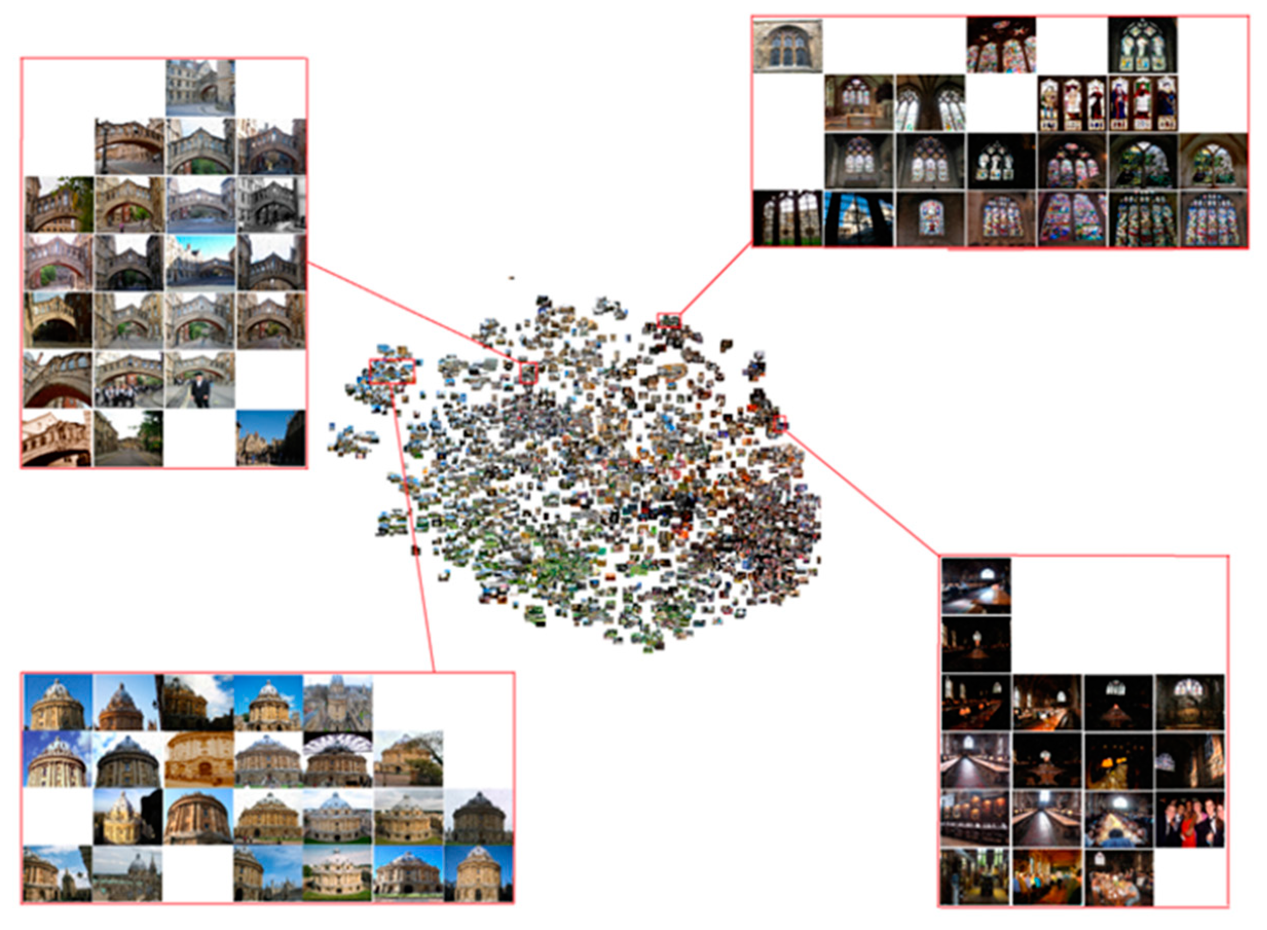
Figure 8.
Barnes–Hut t-SNE (t-distributed stochastic neighbor embedding) [41] visualization of the learned embedding feature on the oxford5k data set [33].


Table 1.
Performance (mean average precision (mAP)) comparison between regional maximum activation of convolutions (R-MAC) [25] and generalized R-MAC (GR-MAC) on the Paris6k, Oxford5k, and Holidays data sets. The best result is highlighted in bold.
Table 1.
Performance (mean average precision (mAP)) comparison between regional maximum activation of convolutions (R-MAC) [25] and generalized R-MAC (GR-MAC) on the Paris6k, Oxford5k, and Holidays data sets. The best result is highlighted in bold.
| Method | Oxford5k | Paris6k | Holidays |
|---|---|---|---|
| R-MAC [25] | 66.85 | 82.24 | 88.88 |
| GR-MAC | 70.35 | 83.62 | 89.58 |
Table 2.
Performance (mAP) comparison between regional maximum activation of convolutions (R-MAC) [25] and generalized R-MAC (GR-MAC) on ROxford and RParis data sets. The best result is highlighted in bold.
Table 2.
Performance (mAP) comparison between regional maximum activation of convolutions (R-MAC) [25] and generalized R-MAC (GR-MAC) on ROxford and RParis data sets. The best result is highlighted in bold.
| Method | Easy | Medium | ||||||||||
|---|---|---|---|---|---|---|---|---|---|---|---|---|
| ROxford | RParis | ROxford | RParis | |||||||||
| mAP | P@1 | P@5 | mAP | P@1 | P@5 | mAP | P@1 | P@5 | mAP | P@1 | P@5 | |
| R-MAC GR-MAC | 58.74 63.33 | 83.82 85.29 | 73.97 78.24 | 78.50 80.15 | 95.71 95.71 | 93.43 93.71 | 39.40 42.26 | 84.29 84.29 | 67.14 70.19 | 61.56 63.86 | 95.71 95. 71 | 96.26 96.29 |
Table 3.
Performance (mAP) comparison of cross-dimensional weighting (Crow) [26] and saliency joint weighting (SJW) on the Paris6k, Oxford5k, and Holidays data sets. The best result is highlighted in bold.
Table 3.
Performance (mAP) comparison of cross-dimensional weighting (Crow) [26] and saliency joint weighting (SJW) on the Paris6k, Oxford5k, and Holidays data sets. The best result is highlighted in bold.
| Method | Oxford5k | Paris6k | Holidays |
|---|---|---|---|
| Crow [26] | 68.09 | 77.88 | 89.50 |
| SJW | 69.62 | 79.41 | 89.74 |
Table 4.
Performance (mAP) comparison between cross-dimensional weighting (Crow) [26] and saliency joint weighting (SJW) on the ROxford and RParis data sets. The best result is highlighted in bold.
Table 4.
Performance (mAP) comparison between cross-dimensional weighting (Crow) [26] and saliency joint weighting (SJW) on the ROxford and RParis data sets. The best result is highlighted in bold.
| Method | Easy | Medium | ||||||||||
|---|---|---|---|---|---|---|---|---|---|---|---|---|
| ROxford | RParis | ROxford | RParis | |||||||||
| mAP | P@1 | P@5 | mAP | P@1 | P@5 | mAP | P@1 | P@5 | mAP | P@1 | P@5 | |
| Crow SJW | 61.23 63.09 | 85.29 88.24 | 75.00 75.00 | 77.46 78.68 | 97.14 97.14 | 92.57 93.71 | 46.10 47.36 | 87.14 87.14 | 72.38 72.57 | 59.99 60.90 | 97.14 97.14 | 95.14 96.00 |
Table 5.
Performance (mAP) comparison using query expansion or not. QE: using query expansion (+QE). We use bold colors to highlight the best result. GSW, global saliency weighted.
Table 5.
Performance (mAP) comparison using query expansion or not. QE: using query expansion (+QE). We use bold colors to highlight the best result. GSW, global saliency weighted.
| Method | Dim | Oxford5k | Paris6k | Holidays |
|---|---|---|---|---|
| Original retrieval results | ||||
| GR-MAC | 512 | 70.35 | 83.62 | 89.58 |
| SJW | 512 | 69.62 | 79.41 | 89.74 |
| GSW | 512 | 72.90 | 83.60 | 90.56 |
| After query expansion (QE) | ||||
| GR-MAC+QE | 512 | 79.20 | 89.86 | 90.36 |
| SJW+QE | 512 | 74.79 | 86.17 | 89.53 |
| GSW+QE | 512 | 79.87 | 89.55 | 91.51 |
Table 6.
Performance (mAP) comparison with the state-of-the-art algorithms in Oxford5k, Paris6k and Holidays. Dim: dimensionality of final compact image feature descriptors. QE: using query expansion (+QE). The best result is highlighted in bold. SPoC, simplest sum-pooled convolutional; MFC, multiscale fully convolutional; MAC, maximum activation of convolutions; GeM, generalized-mean pooling; FDE, fusing feature distribution entropy; SBA, semantic-based aggregation; BoW, bag-of-visual words.
| Method | Dim | Oxford5k | Paris6k | Holidays |
|---|---|---|---|---|
| Original retrieval results | ||||
| SPoC [23] | 256 | 53.10 | - | 80.20 |
| MFC [27] | 256 | 68.40 | 83.40 | - |
| MAC [28] | 512 | 55.01 | 74.73 | 75.23 |
| SPoC [23] | 512 | 56.40 | 72.30 | 79.00 |
| MFC [27] | 512 | 70.60 | 83.30 | - |
| R-MAC [25] | 512 | 66.71 | 83.02 | 84.04 |
| GeM [7] | 512 | 67.90 | 74.80 | 83.20 |
| Crow [26] | 512 | 70.80 | 79.70 | 85.10 |
| FDE [39] | 512 | 69.64 | 83.56 | 85.90 |
| SBA [29] | 512 | 72.00 | 82.30 | - |
| GSW (ours) | 512 | 72.90 | 83.60 | 90.56 |
| After query expansion (QE) | ||||
| Crow+QE [26] | 512 | 74.90 | 84.80 | 88.46 |
| MAC+QE [24] | 512 | 74.21 | 82.84 | - |
| R-MAC+QE [25] | 512 | 77.33 | 86.45 | 90.94 |
| FDE+QE [39] | 512 | 78.48 | 86.53 | - |
| BoW-CNN+QE [40] | 512 | 78.80 | 84.80 | - |
| SBA+QE [29] | 512 | 74.80 | 86.00 | - |
| GSW(ours)+QE | 512 | 79.87 | 89.55 | 91.51 |
Table 7.
Performance (mAP) comparison with the state-of-the-art algorithms on the ROxford and RParis data sets. Dim: dimensionality of the final compact image feature descriptors. QE: using query expansion (+QE). The best result is highlighted in bold.
Table 7.
Performance (mAP) comparison with the state-of-the-art algorithms on the ROxford and RParis data sets. Dim: dimensionality of the final compact image feature descriptors. QE: using query expansion (+QE). The best result is highlighted in bold.
| Method | Easy | Medium | ||||||||||
|---|---|---|---|---|---|---|---|---|---|---|---|---|
| ROxford | RParis | ROxford | RParis | |||||||||
| mAP | P@1 | P@5 | mAP | P@1 | P@5 | mAP | P@1 | P@5 | mAP | P@1 | P@5 | |
| MAC [24] | 44.34 | 72.06 | 60.59 | 63.39 | 92.86 | 90.29 | 32.20 | 71.43 | 56.29 | 49.09 | 94.29 | 93.14 |
| SPoC [23] | 44.31 | 67.65 | 56.54 | 68.06 | 92.86 | 91.71 | 30.33 | 65.71 | 49.71 | 50.92 | 92.86 | 94.57 |
| R-MAC [25] | 58.74 | 83.82 | 73.97 | 78.50 | 95.71 | 93.43 | 39.40 | 84.29 | 67.14 | 61.56 | 95.71 | 96.26 |
| GeM [7] | 58.83 | 85.29 | 75.74 | 76.85 | 94.29 | 92.29 | 42.68 | 87.14 | 72.29 | 60.80 | 97.14 | 95.14 |
| Crow [26] | 61.23 | 85.29 | 75.00 | 77.46 | 97.14 | 92.57 | 46.10 | 87.14 | 72.38 | 59.99 | 97.14 | 96.00 |
| GR-MAC (ours) | 63.33 | 85.29 | 78.24 | 80.15 | 95.71 | 93.71 | 42.26 | 84.29 | 70.19 | 63.86 | 95.71 | 96.29 |
| SJW (ours) | 63.09 | 88.24 | 75.00 | 78.68 | 97.14 | 93.71 | 47.36 | 87.14 | 72.57 | 60.90 | 97.14 | 96.00 |
| GSW (ours) | 66.70 | 88.24 | 80.00 | 81.43 | 95.71 | 94.10 | 48.13 | 88.57 | 75.05 | 64.68 | 95.71 | 96.57 |
| After query expansion (QE) | ||||||||||||
| MAC+QE | 53.03 | 73.53 | 64.41 | 78.98 | 92.86 | 90.57 | 38.62 | 72.86 | 60.29 | 64.50 | 92.86 | 93.14 |
| R-MAC+QE | 75.04 | 88.24 | 84.04 | 88.20 | 95.71 | 95.14 | 53.59 | 85.71 | 75.90 | 73.13 | 97.14 | 96.29 |
| GeM+QE | 68.12 | 89.71 | 81.47 | 85.87 | 94.29 | 93.14 | 51.29 | 88.57 | 76.00 | 71.13 | 95.71 | 95.71 |
| Crow+QE | 65.98 | 85.29 | 78.53 | 83.61 | 95.71 | 94.86 | 48.88 | 84.29 | 74.14 | 66.25 | 97.14 | 97.14 |
| GSW+QE | 76.17 | 91.18 | 85.29 | 88.34 | 95.71 | 96.00 | 55.22 | 88.57 | 79.71 | 72.48 | 97.14 | 97.43 |
Table 8.
The result with different scale size L. The maximum value is in bold.
| L | 1 | 2 | 3 | 4 |
|---|---|---|---|---|
| R-MAC [25] | 56.34 | 63.09 | 66.85 | 67.79 |
| GR-MAC | 65.13 | 70.03 | 70.35 | 70.07 |
Table 9.
The influence of n on retrieval. The maximum value is in bold.
| 10% | 20% | 30% | 40% | 50% | 60% | 70% | 80% | 90% | 100% | |
|---|---|---|---|---|---|---|---|---|---|---|
| mAP | 69.23 | 69.58 | 69.62 | 69.57 | 69.44 | 69.33 | 69.29 | 69.23 | 69.23 | 69.21 |
Table 10.
The influence of on retrieval. The maximum value is bolded.
| 1 | 10 | 100 | 500 | |
|---|---|---|---|---|
| mAP | 69.41 | 69.51 | 69.62 | 68.60 |
Table 11.
The influence of on retrieval. The maximum value is bolded.
| α | β | mAP |
|---|---|---|
| 0.1 | 0.9 | 70.75 |
| 0.2 | 0.8 | 71.62 |
| 0.3 | 0.7 | 72.37 |
| 0.4 | 0.6 | 72.60 |
| 0.5 | 0.5 | 72.85 |
| 0.6 | 0.4 | 72.90 |
| 0.7 | 0.3 | 72.62 |
| 0.8 | 0.2 | 70.61 |
| 0.9 | 0.1 | 68.78 |
Publisher’s Note: MDPI stays neutral with regard to jurisdictional claims in published maps and institutional affiliations. |
© 2021 by the authors. Licensee MDPI, Basel, Switzerland. This article is an open access article distributed under the terms and conditions of the Creative Commons Attribution (CC BY) license (https://creativecommons.org/licenses/by/4.0/).
Share and Cite
MDPI and ACS Style
Zhao, H.; Wu, J.; Zhang, D.; Liu, P. Toward Improving Image Retrieval via Global Saliency Weighted Feature. ISPRS Int. J. Geo-Inf. 2021, 10, 249. https://0-doi-org.brum.beds.ac.uk/10.3390/ijgi10040249
AMA Style
Zhao H, Wu J, Zhang D, Liu P. Toward Improving Image Retrieval via Global Saliency Weighted Feature. ISPRS International Journal of Geo-Information. 2021; 10(4):249. https://0-doi-org.brum.beds.ac.uk/10.3390/ijgi10040249
Chicago/Turabian StyleZhao, Hongwei, Jiaxin Wu, Danyang Zhang, and Pingping Liu. 2021. "Toward Improving Image Retrieval via Global Saliency Weighted Feature" ISPRS International Journal of Geo-Information 10, no. 4: 249. https://0-doi-org.brum.beds.ac.uk/10.3390/ijgi10040249
Note that from the first issue of 2016, this journal uses article numbers instead of page numbers. See further details here.