Article

Comparison of Machine Learning Methods for Potential Active Landslide Hazards Identification with Multi-Source Data

1
Aerospace Information Research Institute, Chinese Academy of Sciences, Beijing 100094, China
2
University of Chinese Academy of Sciences, Beijing 100049, China
3
China Aero Geophysical Survey & Remote Sensing Center for Natural Resources, Beijing 100083, China
4
Key Laboratory of Earth Observation Hainan Province, Sanya 572029, China
5
Sanya Institute of Remote Sensing, Sanya 572029, China
*
Author to whom correspondence should be addressed.
These authors contributed equally to this work.
ISPRS Int. J. Geo-Inf. 2021, 10(4), 253; https://0-doi-org.brum.beds.ac.uk/10.3390/ijgi10040253
Submission received: 28 February 2021 / Revised: 21 March 2021 / Accepted: 6 April 2021 / Published: 9 April 2021
(This article belongs to the Special Issue Disaster Management and Geospatial Information)

Abstract

:
The early identification of potential landslide hazards is of great practical significance for disaster early warning and prevention. The study used different machine learning methods to identify potential active landslides along a 15 km buffer zone on both sides of Jinsha River (Panzhihua-Huize section), China. The morphology and texture features of landslides were characterized with InSAR deformation monitoring data and high-resolution optical remote sensing data, combined with 17 landslide influencing factors. In the study area, 83 deformation accumulation areas of potential landslide hazards and 54 deformation accumulation areas of non-potential landslide hazards were identified through spatial overlay analysis with 64 potential active landslides, which have been confirmed by field verification. The Naive Bayes (NB), Decision Tree (DT), Support Vector Machine (SVM) and Random Forest (RF) algorithms were trained and tested through attribute selection and parameter optimization. Among the 17 landslide influencing factors, Drainage Density, NDVI, Slope and Weathering Degree play an indispensable role in the machine learning and recognition of landslide hazards in our study area, while other influencing factors play a certain role in different algorithms. A multi-index (Precision, Recall, F1) comparison shows that the SVM (0.867, 0.829, 0.816) has better recognition precision skill for small-scale unbalanced landslide deformation datasets, followed by RF (0.765, 0.756, 0.741), DT (0.755, 0.756, 0.748) and NB (0.659, 0.659, 0.659). Different from the previous study on landslide susceptibility and hazard mapping based on machine learning, this study focuses on how to find out the potential active landslide points more accurately, rather than evaluating the landslide susceptibility of specific areas to tell us which areas are more sensitive to landslides. This study verified the feasibility of early identification of landslide hazards by using different machine learning methods combined with deformation information and multi-source landslide influencing factors rather than by relying on human–computer interaction. This study shows that the efficiency of potential hazard identification can be increased while reducing the subjective bias caused by relying only on human experts.

1. Introduction

Landslides are a type of geological disaster that can cause serious casualties and huge property losses [1,2]. The special topographical and geomorphological features of southwest China, such as high elevations, numerous mountains, steep slopes, deep valleys, broken rock and soil, have created numerous slopes and cutting surfaces with sufficient sliding potential. These slopes form the basic conditions for landslides which occur frequently [1]. Among them, the Baige landslide in October and November 2018 in the Jinsha River Valley caused huge losses in the middle and lower reaches of the Jinsha River [2].
In the research field of landslides, the early identification of potential landslide hazards is a hot but difficult topic [3,4]. In general, landslides have obvious spatio-temporal characteristics. Spatially, the study of landslides can be considered at regional and point scales. Temporally, the study of landslides can either focus on the time they have occurred or on potential landslide hazards [4,5,6]. Regional-scale studies mainly focus on three aspects: landslide detection, historical landslide cataloging, and regional landslide risk assessment. These regional-scale studies rely on spectral features, spatial features, morphological attributes, and contextual information of landslides derived from multi-source remote sensing images. These studies often use Object-Oriented methods, SVM, RF and other machine learning methods to identify the occurrence of landslides and cataloging them; the regional landslide risk assessment is then realized by different machine and ensemble learning models by modeling and analyzing the importance of influencing factors of landslide cataloging, and obtain landslide susceptibility maps [7,8,9,10,11,12]. Point-scale studies focus on retrospective analyses of the spatio-temporal evolution of a specific landslide disaster and provide data for monitoring an emergency and analyze a landslide disaster. These studies are more often based on optical or radar remote sensing and are useful for monitoring and early warning of landslide disaster risks, disaster evolution, pre-disaster creep characteristics and post-disaster secondary hazards [6,13,14]. In recent years, due to the great advances in InSAR technology in the field of surface deformation monitoring, studies started to use time series of radar interferometry of repeated orbit observations for studying regional active landslide hazards and obtaining potential landslide hazards data through human–computer interaction interpretation [15,16]. However, Previous studies often did not take advantage of data mining analysis of InSAR deformation results and of all the factors influencing potential active landslide hazards and did not establish a relationship between the extent of surface deformation and the causal factors, because the active landslide identification based on deformation results has been more completed through human–computer interaction interpretation. Machine learning may provide a better solution to distinguish which deformation accumulation areas are landslide hazards and non-landslide hazards, which is a more complex problem. Compared with traditional methods, machine learning methods can fit complex multiple interactions or nonlinear relationships, which brings a higher prediction accuracy. Machine learning methods are often a good supplement to the traditional statistical methods, and even a good substitute in many cases. Besides, studies show that compared with statistical regression or machine learning models, ensemble learning can improve the accuracy of landslide sensitivity mapping to a certain extent, which needs more complex model optimization and adjustment. At the same time, different methods have great differences in data samples, influencing factors selection, parameter adjustment, model robustness and generalization [17,18,19,20,21,22,23,24,25,26,27,28,29]. An urgent problem in the field of landslide monitoring and risk assessment is to define how to analyze and mine landslide risk factors applying machine learning to multi-source remote sensing, basic geography, and geological data, and how to establish or choose recognition models for early warning of potential landslide hazards based on deformation data.
Surface deformation results at different scales can be used to analyze landslides in various active stages. The results obtained with InSAR data play an important role in early warning of active landslides. The coherence and imaging geometry required by InSAR make it suitable for active landslide identification in the middle and lower reaches of Jinsha River with typical dry-hot valley characteristics [2]. Therefore, the study selected a 15 km buffer zone on both sides of the Jinsha River valley to identify potential landslide hazards. Based on the field investigation results of landslide hazards, InSAR surface deformation data, terrain, landform, geological environment, vegetation indices and other related multi-source factors of landslides, through spatial analysis and regional mean statistics, the multi-source features-fusion-dataset including landslide and non-landslide was constructed. And then, the study used four different machine learning methods to detect active potential landslide hazards after feature selection and parameter optimization. The classification accuracy was compared and analyzed to identify the optimal classification method for the early identification of active landslide hazards based on deformation accumulation data.

2. Materials and Methods

2.1. Study Area

The study area was located in the middle and lower reaches (Panzhihua-Huize section) of Jinsha River, China. This section lies flows through the Hengduan Mountains and has complex geological conditions. The strata are mainly composed of presinian metamorphic rocks, Mesozoic coal measures strata, red beds and Permian strata. Faults and folds are well developed in the study area, mainly in the North-South (NS), North-East (NE), and North-North-East (NNE) directions. The geomorphological types are mainly middle-high mountain valleys, then middle mountain and rift basins. The altitude of the mountains ranges between 2000 and 3500 m, and the valley bottom is between 500 and 900 m.
The study area is a typical dry hot valley in China, which is controlled by tropical continental monsoon climate. Intense solar radiation leads to rapid evaporation in this area. The average daily temperature is 18~20 °C, the annual accumulated temperature is generally 6000~7500 °C, which refers to the sum of the daily average temperature in a period of time ≥10 °C. The annual precipitation is about 800 mm, which is one-third of the annual evaporation, the water-heat matching is seriously unbalanced. The unique landform with steep terrain and deep valley leads to a hot and arid climate in Jinsha River, with relatively low vegetation development on both sides of the banks. In addition, due to mineral development and steep slope reclamation, the surface vegetation is sparse and the soil layer is exposed; the geological conditions are extremely unstable in the study area, where is at high-risk of geological disasters. The unique characteristics of the study area are suitable for the differential phase timing analysis method of InSAR based on coherent targets.
Figure 1 show the remote sensing image of GaoFen-1 (GF-1) Satellite.

2.2. Data

The data sources of this study included radar remote sensing data, optical remote sensing data, landform data, basic geographic information data, basic geological data and land cover data. The details of the data source are shown in Table 1.
Figure 2 and Figure 3 show the PS-InSAR results of the ascending and descending deformation from Sentinel-1 in the study area. As the introduction of Section 2.1 study area, the PS-InSAR method is suitable for the surface deformation monitoring work in the study area, and the calculated results are verified in the field, which are in good agreement with the local actual situation. Other data will be introduced in Section 2.3.2 influencing factors of landslide section.
Based on the multi period Sentinel-1 data and Gaofen-1 optical image in the data list of Table 1, the temporal InSAR processing method and human–computer interactive interpretation method based on expert experience were used respectively to obtain the spatial distribution of deformation accumulation area and suspected active landslide hazards in the study area. In order to ensure the identification accuracy of active landslide hazards in the study area, the study introduced overlapping area inspection and external observation calibration in the process of time series InSAR data processing, and carried out field verification on the identification results of 23 suspected active landslide hazards, of which 16 were identified as active landslide hazards, and the overall identification accuracy of active landslide hazards in the study area was 69.57%, which shows that the potential active landslide hidden danger data obtained has reached a high accuracy, because what the study focused on is not occurred landslides, but the discrimination and prediction of the potential landslide hidden danger that has not yet occurred. Then, based on the new understanding of disaster conditions and optical remote sensing characteristics of landslides obtained from field verification, the identification results of suspected active landslide hazards were revised, and 64 typical active landslide hazards in the study area were finally determined. At the same time, with the help of spatial overlay analysis, the deformation accumulation areas indicating landslide hazards and non-landslide hazards were distinguished, which provides an important data basis for the construction of the dataset. Furthermore, based on the Landsat-8, Geology, DEM, DLG and Globeland30 data in the data list of Table 1, this study calculated 17 kinds of landslide hazard characteristic data results. In order to construct a spatial scale consistent feature dataset of active landslide hazard identification for model training and validation, the spatial grid size of multi-source data were assimilated to 30 m ∗ 30 m. The process of an active landslide hazard identification feature dataset will be introduced in Section 2.3. Figure 4 is the example of field verification results of suspected active landslide hazards.

2.3. Methods

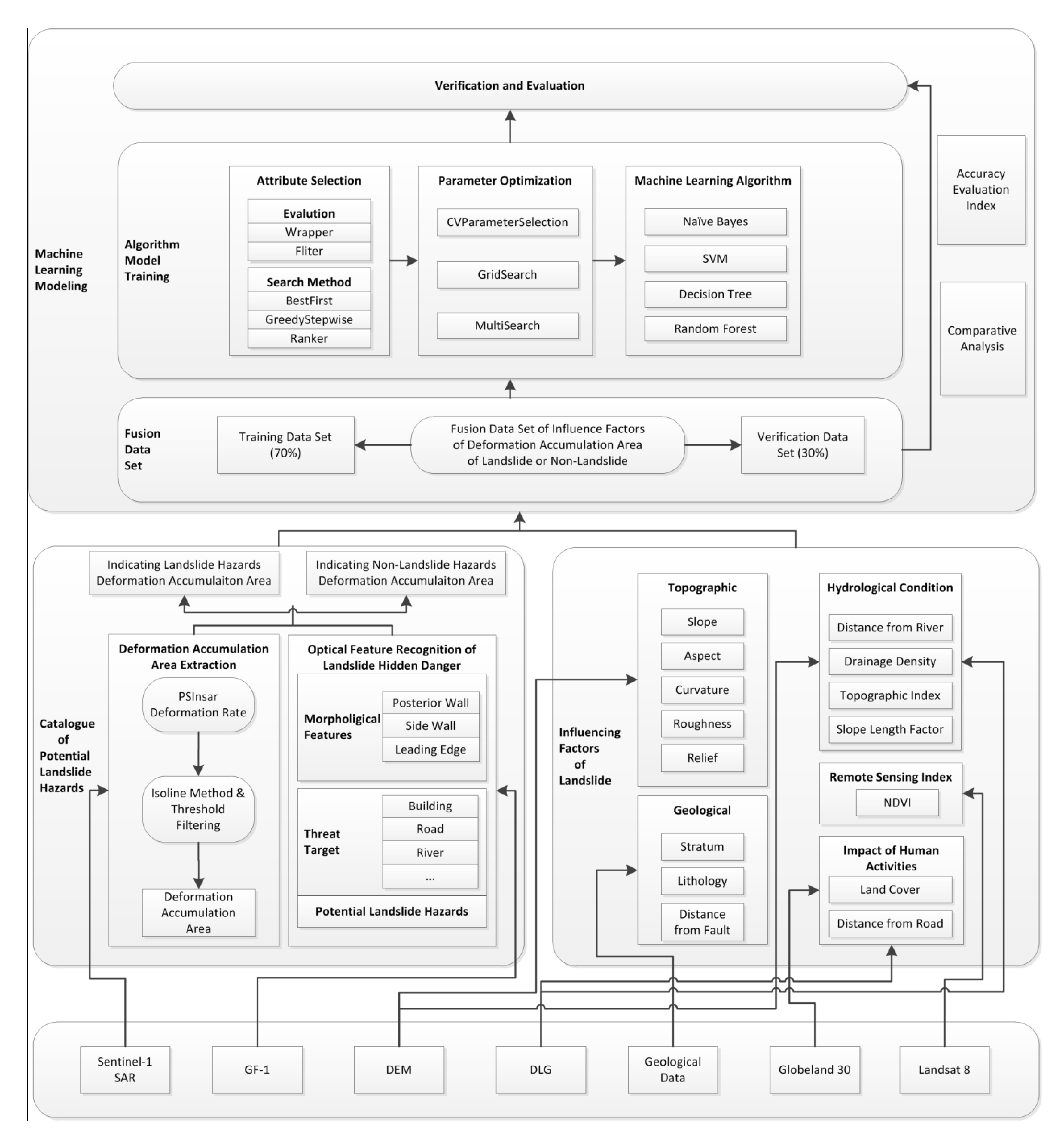
With the help of InSAR deformation data, high-resolution optical remote sensing data, geological background and other multi-source data combined with ground survey data, this study carried out a comprehensive investigation of the active landslide hazards in the study area following the discrimination principle of deformation, shape and threat. Based on the potential landslide hazards and the typical deformation accumulation area filtered by an isoline threshold, 137 data records of potential and non-potential landslide hazards were recorded, including 83 records of deformation accumulation area and 54 records of non-landslide deformation accumulation area. The multi-source attribute characteristics of 137 deformation accumulation areas were extracted by calculating and extracting landslide influencing factors such as landform, basic geology, hydrological conditions, and NDVI. Training sets (n = 96, 70%) and validation sets (n = 41, 30%) were randomly established. Four machine-learning methods, namely NB, DT, SVM and RF, were trained to identify potential landslide hazards after attribute selection and parameter optimization. Finally, the optimal model of potential landslide hazard identification in the study area, which is indicated by the deformation accumulation area, was obtained through the verification and comparison evaluation. The overall study methodology flow is shown in Figure 5.

2.3.1. Catalogue of Potential Landslide Hazards

Identifying landslide risk is the basis of recognizing potential landslide hazards by machine learning. The deformation accumulation area is the key factor determining the potential landslide hazard. Based on surface deformation data, a total of 137 deformation areas were identified by delineating and filtering the deformation concentration areas. A total of 64 potential landslide hazards were identified by using high-resolution optical remote sensing images to analyze the morphological features and hazards surrounding the deformable areas. These steps were carried out through human–computer interactive interpretation and field investigation combined with expert knowledge. The specific location and spatial distribution of deformation accumulation areas and potential landslide hazards in the study area are shown in Figure 6.

2.3.2. Influencing Factors of Landslide

The occurrence of landslides is often related to geological factors, hydrological conditions, topography, land cover, human activities, and so on. The published literature on landslide sensitivity at global or regional scale identifies a number of factors related to the occurrence of landslides. These factors include elevation, slope, aspect, curvature, geology, structure, land cover, distance from rivers and roads, among others [1,26].
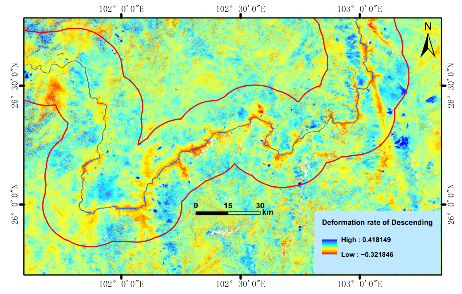
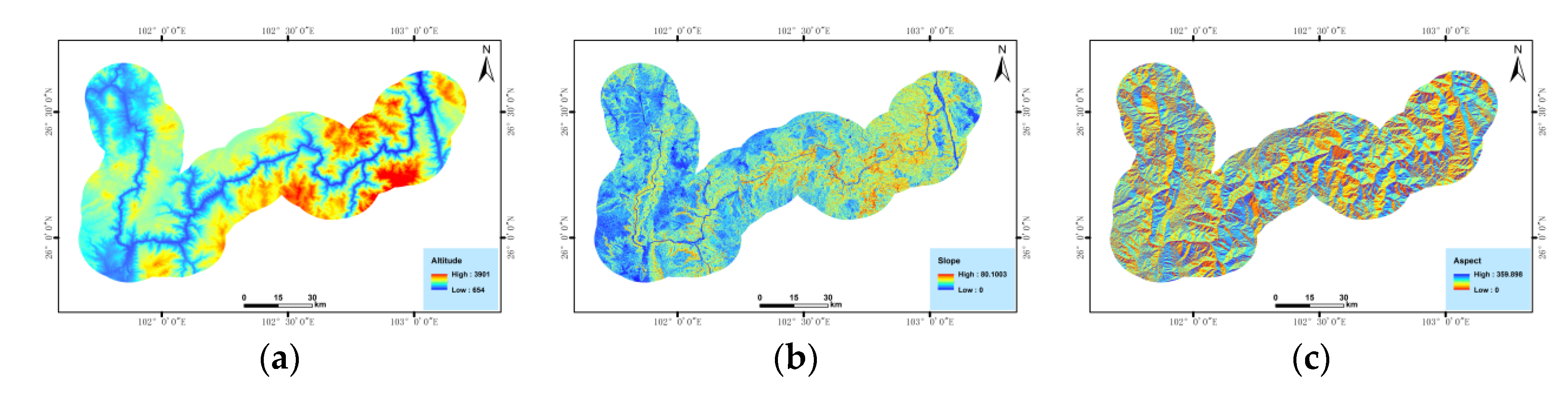
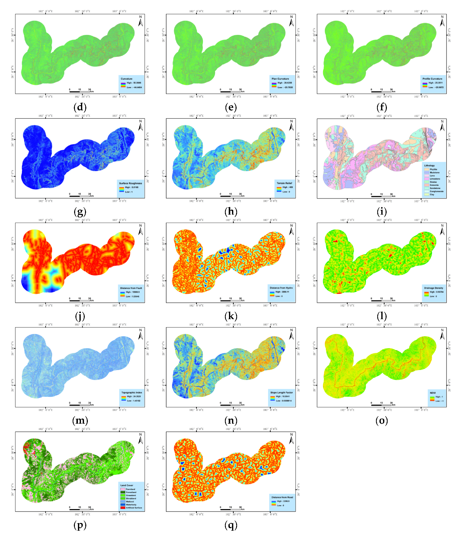
In addition to the optical remote sensing image data and InSAR deformation monitoring data, this study identified 17 influencing factors, including topography, geological background, hydrological conditions, remote sensing data, and human activities as input variables to the machine learning algorithms to perform a “data driven” landslide hazard identification rather than an “expert experience-driven” landslide evaluation and analysis, as shown in Figure 7 and Table 2. Table 2 also showed the numerical statistics (Mean, Minimum, Maxi-mum) of landslide area in the study area. The processing of the 17 factors in the dataset was implemented in ArcGIS 10.5.
Then, based on Section 2.3.1 and Section 2.3.2, the study calculated the attribute fusion dataset of surface deformation area by a zonal mean statistics method, which can transform the polygon-based surface deformation area into samples.
Generally, in terms of topography and geomorphology, a moderately gentle land-form with a steep top is prone to landslide development. In terms of geological back-ground, landslide development is mainly affected by the angle of the strata and by the geological structure. Different strata present different hardness, compactness and susceptibility to weathering, and contribution of material to a landslide. Slope discontinuities caused by a fault in the structural plane create the conditions for landslide occurrence. Hydrological conditions are the main determinants for the development of landslides. The difference between active landslides and rainfall-induced landslides lies in the softening of rocks and soil caused by the long-term action of surface water and groundwater, which reduces the strength of rocks and soil, produces hydrodynamic pressure and pore water pressure, increases the bulk density of rock and soil mass, and produces buoyancy forces on permeable strata, especially on the sliding surface (zone), which reduces the strength of the composite. Changes in land cover and the influence of human activities also promote the formation of landslides, especially the destruction of vegetation, excavation at the base of a slope, slope accumulation and other risky human engineering activities are among the important factors affecting the occurrence of landslides.

2.3.3. Machine Learning Algorithms

The following is a brief introduction to the four machine learning methods used in this study.
  • Naive Bayes
Naive Bayes is a statistical analysis machine learning algorithm based on Bayes criterion. It uses the “attribute conditional independence assumption” to construct a classifier from a probability model and determine the maximum posterior probability (MAP) decision criterion, so as to realize the optimal decision classification for uncertain factors.
Assume an item to be classified as X = f1, f2, ⋯, fn, where each f is a characteristic attribute of X, and the category set is C1, C2, ⋯, Cm, calculate conditional probability separately P(fn|Cm). If P(Ck|X) = MAX(P(C1|X),P(C2|X),…,P(Cm|X)), then XCk, the one with the largest probability is the Bayesian classification result. Naive Bayes assumes that each feature is independent, according to Bayes’ theorem, it can be derived: P(Ci|X) = P(X|Ci)P(Ci)/P(X) [30]. Finally, the classifier formula corresponding to the Naive Bayes algorithm is defined as follows:
c l a s s i f y ( f 1 , , f n ) = a r g m a x   p ( C = c ) i n p ( F i = f i | C = c )
Among them, fn is the characteristic attribute of X, p(C) is the prior probability, and p(F|C) is the posterior probability.
2.
Decision Tree
Decision Tree uses one of the characteristic attributes of the sample data as the classification condition, divides the sample into two subsets, and then continuously loops the classification until each subset belongs to the same label. The tree structure can effectively handle the classification problem. The key to building a Decision Tree is feature-selected. Common feature selection algorithms for a Decision Tree include ID3, C4.5 and CART. Among them, the core of the ID3 algorithm is to apply information gain criteria on each node of the decision tree to select features, and recursively build the decision tree; the C4.5 algorithm is similar to the ID3 algorithm decision tree generation process, and it improves the ID3 algorithm, the maximum information gain rate (ratio) is used to select features; the CART algorithm will be introduced in the random forest section [31].
This research uses the C4.5 Decision Tree algorithm. The split information defined by the algorithm is as follows, which is a definition of entropy:
split _ info A ( D ) = j = 1 v | D j | | D | log 2 | D j | | D |
According to the above formula, the information gain rate formula defined by the C4.5 algorithm is as follows:
gain _ ratio ( A ) = g a i n ( A ) s p l i t _ i n f o ( A )
3.
Support Vector Machine
Support Vector Machine aims to obtain a separation hyperplane that correctly divides the dataset and has the largest geometric interval through nonlinear transformation. The largest separation boundary is the support vector. The classification results of SVM depend on the selection of different kernel functions, such as polynomial functions, sigmoid functions, and radial basis functions [32]. The kernel function used in this study was a radial basis function.
The basic idea of SVM is to calculate the separating hyperplane: w × x + b = 0, where w is the normal vector and b is the intercept. For a linearly separable dataset, there are infinitely many such hyperplanes which are perceptrons, but the separating hyperplane with the largest geometric interval is unique. For nonlinear classification problems, it can be transformed into a linear classification problem in a certain dimensional feature space by nonlinear transformation, and linear support vector machines can be learned in the high-dimensional feature space. Because of the dual problem of linear SVM, the objective function and the classification decision function only involve the inner product between the instance and the instance, so there is no need to explicitly specify the nonlinear transformation, but the inner product is replaced by the kernel function [32,33,34]. Specifically, K(x,z) is a function, which means that there is a mapping ɸ(x) from the input space to the feature space. For x, z in any input space,
K ( x , z ) = ( x ) ( z )
In the dual problem of linear SVM learning, replacing the inner product with the kernel function K(x,z), the result is nonlinear SVM:
f ( x ) = s i g n ( i = 1 N α i * y i K ( x , x i ) + b * )
4.
Random Forest
Random Forest is considered to be one of the most effective non-parametric ensemble learning methods in the field of machine learning. It is based on the Bagging strategy, introduces random attributes in the training process, and uses training datasets to generate multiple deep decision trees. Each decision tree that constitutes a random forest will predict an output result, which is determined by the weighted calculation of the number of votes. The majority vote of an output result and the degree of convergence of the fitting determine the final classification result [35]. Random forests can prevent most overfitting problems by creating random feature subsets and using these subsets to build smaller decision trees, and then forming subtrees.
Specifically, Random Forest is modified on the basis of Bagging. First, use the Bootstrap method to sample n samples from the dataset, then randomly select k attributes from all attributes to build a CART tree, and finally repeat the above steps m times to build m CART trees. These m CART trees form a random forest, and the result of voting determines which category the data belongs to. CART is basically similar to decision tree methods such as ID3.5 and C4.5. The difference is that CART uses Gini coefficient as the criterion for feature selection. The Gini coefficient is essentially an approximation of the information gain. The larger the Gini coefficient of an attribute, the stronger the attribute’s ability to reduce the entropy of the sample. This attribute makes the data stronger, from uncertainty to certainty. The formula is as follows:
Gini ( p ) = k = 1 K p k ( 1 p k ) = 1 k = 1 K p k 2 = 1 k = 1 K ( | C k | | D | ) 2
Before model training, attribute selection and parameter optimization should be carried out first, in order to ensure that different algorithms perform classification tasks under the optimal attribute (subset) set and parameters. A feature evaluation strategy can be divided into Wrapper and Filter; the former focuses on the evaluation of the feature subset, the latter focuses on the evaluation of single attributes. Different evaluation strategies for Wrapper and Filter have different searching methods and attribute selection strategies should be selected according to different algorithms [36,37,38,39,40]. For a specific algorithm, there are three main methods for parameter optimization: CV Parameter Selection, Grid-Search, and Multi Search. The selection principles of parameter optimization methods vary according to the number of parameters to be optimized:
(1) If there are no more than two parameters to be optimized, Grid-search is selected and the boundary is automatically expanded;
(2) If more than two parameters need to be optimized, Multi Search is selected;
(3) If the direct parameters of the classifier are optimized and the number of parameters is no more than two, the CV Parameter Selection can also be considered.
Different parameter optimization methods are chosen according to different algorithms [38]. The attribute selection strategy and the parameter optimization method are shown in Table 3.
The Feature Evaluation Function the study used were WrapperSubsetEval and CorrelationAttributeEval, WrapperSubsetEval evaluates attribute sets by using a learning scheme. Cross validation is used to estimate the accuracy of the learning scheme for a set of attributes [38]; CorrelationAttributeEval evaluates the worth of an attribute by measuring its correlation (Pearson’s) with the class [39].
The Search Strategy the study used were Ranker, BestFirst and GreedyStepwise. Ranker uses an attribute/subset evaluator to rank all attributes. If a subset evaluator is specified, then a forward selection search is used to generate a ranked list. From the ranked list of attributes, subsets of increasing size are evaluated, i.e., the best attribute, the best attribute plus the next best attribute, etc. The best attribute set is reported. RankSearch is linear in the number of attributes if a simple attribute evaluator is used such as GainRatioAttributeEval; BestFirst Searches the space of attribute subsets by greedy Hill_Climbing augmented with a backtracking facility. [40] Setting the number of consecutive non-improving nodes allowed to control the level of backtracking done. Best first may start with the empty set of attributes and search forward, or start with the full set of attributes and search backward, or start at any point and search in both directions (by considering all possible single attribute additions and deletions at a given point); GreedyStepwise performs a greedy forward or backward search through the space of attribute subsets and ay start with no/all attributes or from an arbitrary point in the space. It stops when the addition/deletion of any remaining attributes results in a decrease in evaluation. It can also produce a ranked list of attributes by traversing the space from one side to the other and recording the order that attributes are selected. The Parameter Optimization Methods were CVParameterSelection and GridSearch. CVParameterSelection uses cross validation method, any number of parameters can be optimized; GridSearch is used instead of all the parameter combinations in the experiment to select the parameters, and two parameters can be optimized at most.

2.3.4. Accuracy Assessment

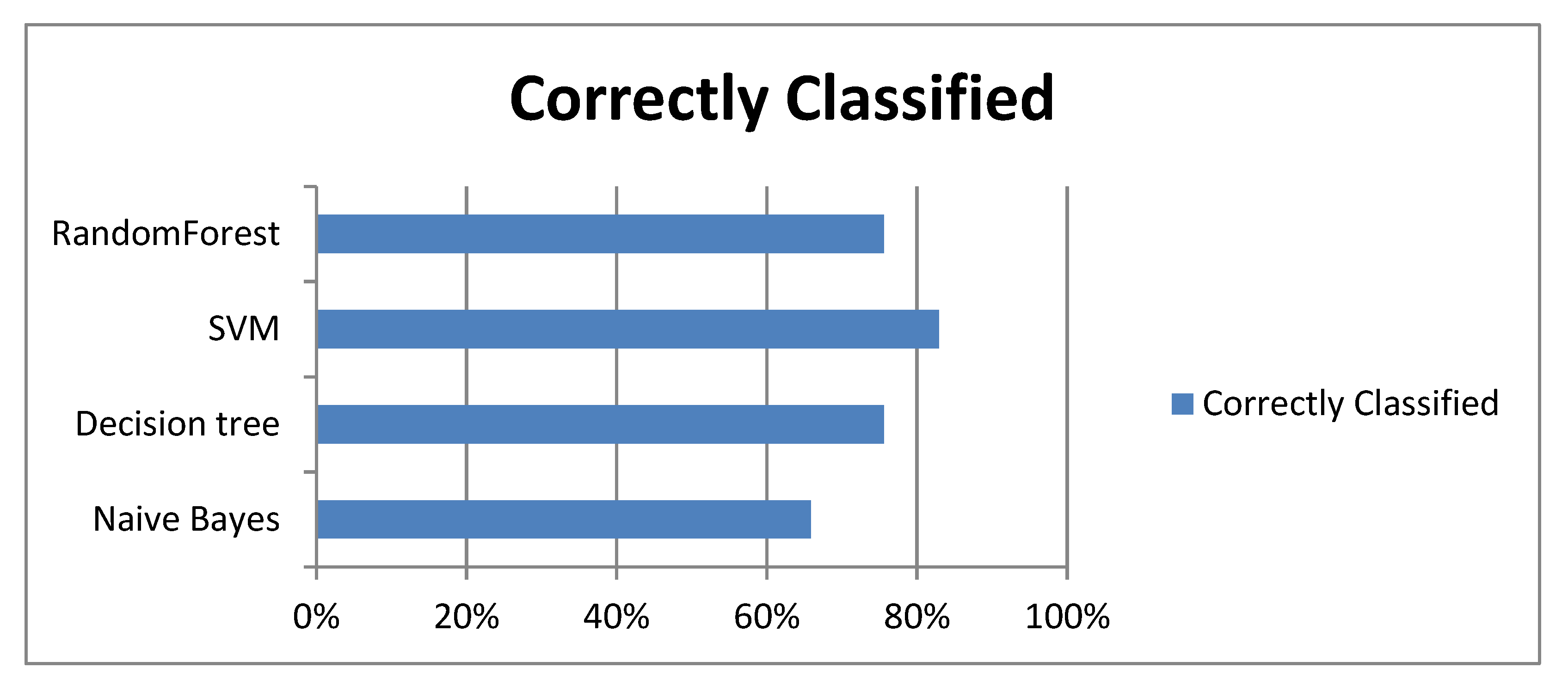
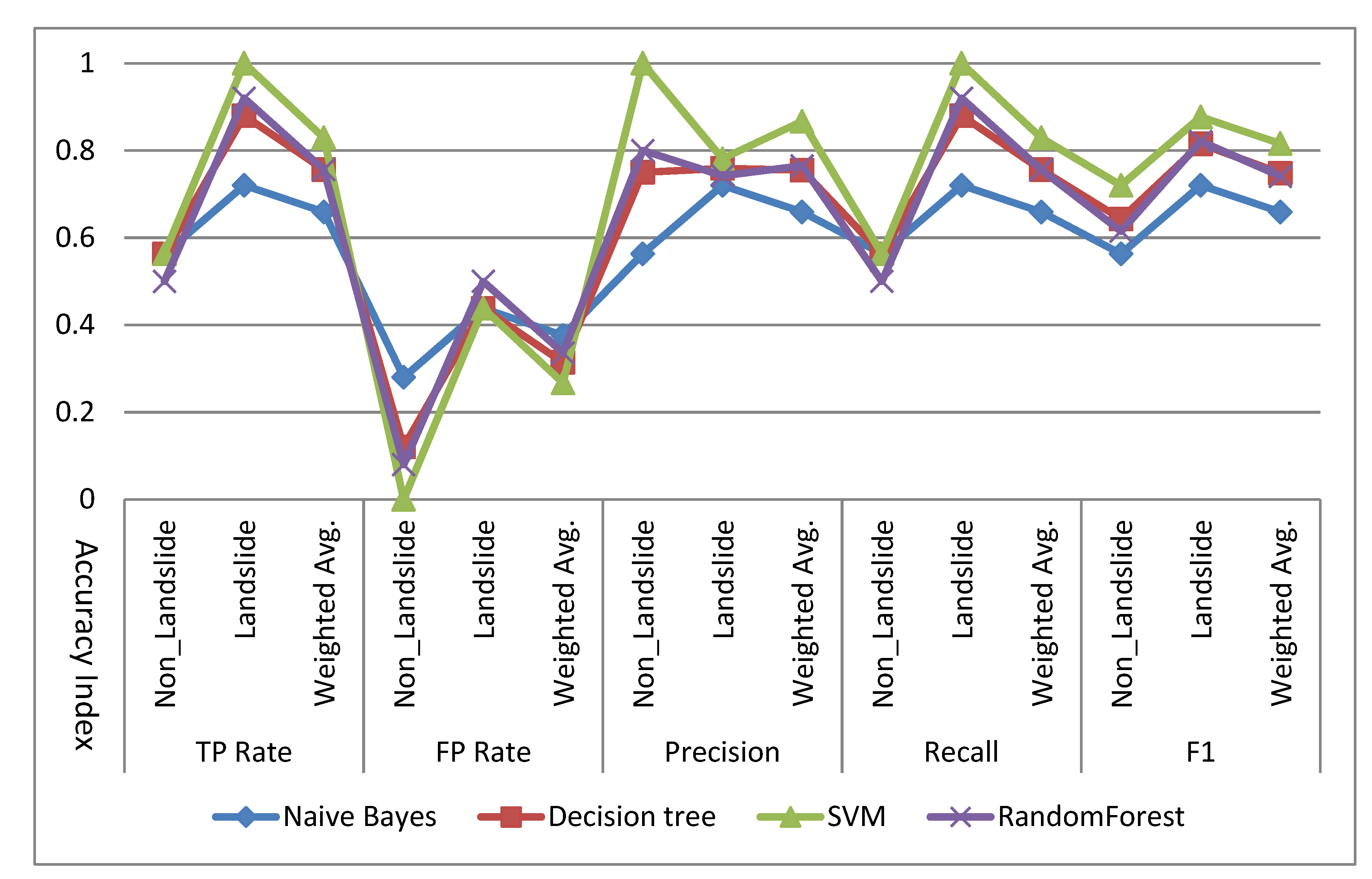
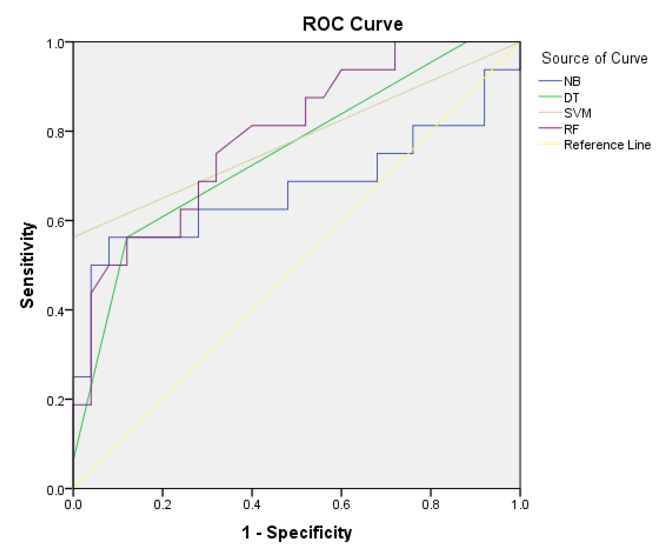
A number of test accuracy indexes of different algorithms were obtained, including Correctly Classified, true positive (TP) rate, false positive (FP) rate, false negative (FN) rate precision, recall, F1, and the AUC (Area Under the ROC curve). Correctly Classified represents the percentage of correct classification, which reflects the correct classification ratio of TP and true negative. TP Rate reflected the proportion of positive samples with correct classification.
Precision is the Precision rate, which is used to measure the ability of the classification algorithm to reject irrelevant information, precision is calculated as:
Precision = TP/(TP + FP)
Recall is the Recall ratio, which is used to measure the ability of classification algorithm to detect relevant information and is calculated as:
Recall = TP/(TP + FN)
F-Measure (F1) is the harmonic mean of precision and recall, and is calculated as:
F-Measure = (2 × Recall × Precision)/(recall + precision) = (2 × TP)/(2 × TP + FP + FN)
AUC is generally greater than 0.5. The closer this value is to 1, the better the classification effect of the model is.

3. Results

Based on the processes illustrated in Figure 6. The study got the attribute selection, classification results and accuracy index of different algorithms with the help of WEKA 3.8.4.

3.1. Attribute Selection Reference Index Results

As can be seen from Table 3, different algorithms adopt different attribute selection strategies. Table 4 shows the reference Pearson product-moment correlation coefficient for the selection of attributes in the NB, and Table 5 shows the cross validation results for DT, SVM, and RF attribute selection. The attribute selection was carried out according to the reference index results of different attribute selection strategies adopted by the algorithm in Table 4 and Table 5. The attributes with a high correlation coefficient were excluded by the NB, and the attributes with “number of folds (%) = 0” were excluded by the DT, SVM and RF.

3.2. Results and Accuracy of Potential Landslide Hazards Identification

The algorithms were trained by using 70% of the data in the deformable cluster attribute fusion dataset and tested on the remaining 30% of the dataset. This paper got the confusion matrix of classification results on test sets, as shown in Table 6 and the prediction results of different methods can be seen in Figure 8.
Based on Table 6, the study got the correctly classified index, as shown in Figure 9, which shows a comparison of the overall correctly classified indexes. The overall correctly classified indexes, from high to low, are SVM > RF = DT > NB. This result indicates that the SVM algorithm performs best in the classification accuracy of the datasets, followed by RF and DT, and the worst performance is with NB.
At the same time, the overall performance, positive sample (Landslide) performance and negative sample (Non-Landslide) performance of different algorithms according to different evaluation indexes of the test set were compared. A number of test accuracy indexes of different algorithms were calculated, including true positive (TP) rate, false positive (FP) rate, false negative (FN) rate precision, recall, and F1 of the algorithms. Table 7 shows the accuracy index results.
As can be seen from Figure 10, SVM had the highest true positive rate in positive and negative samples, the lowest false positive rate in positive and negative samples, the highest Precision rate, the highest recall rate, followed by RF, DT and NB, based on the TP Rate, FP Rate, Precision, Recall and F1.
Algorithms have low accuracy when AUC is 0.5–0.7, and it is more reliable when it is greater than 0.7. Therefore, the study calculated the ROC curve and AUC of the 4 algorithms, and the results are shown in Table 8 and Figure 11. The results show that the RF algorithm has the largest AUC, closely followed by SVM. These were followed by the DT and NB. Thus, it can be seen that, RF, SVM and DT were more reliable.

4. Discussion

In this study, different machine-learning models were applied to multi-source datasets to calculate and predict potential landslide hazards. The extensive use of remote sensing techniques has made data and information from surface deformation and landslide influencing factors (e.g., topography and geology), and their recent situations, available for our perusal. Sentinel-1 SAR data and optical remote sensing data-derived deformation information in the region helped us prepare the inventory map, which was the basis for training and validating the machine-learning algorithms used in this study.
Using available datasets from the study area, 17 influencing factors were calculated. Prior to model training, Pearson correlation factor or 10-fold cross-validation analyses were applied for attribute feature selection of different models. The attribute selection analyses step concluded that different models had different dependence on 17 landslide influencing factors. Next, the training samples of deformation concentration areas with influencing factors were fed into the four machine learning models. Finally, the deformation concentration area were categorized into Landslide/Non-Landslide classes.
The selection of attribute features influences the classification accuracy of the machine-learning algorithm. The same algorithm can have different classification results on different attribute feature subsets, and different algorithms can have different classification results on the same dataset or the same attribute feature subset. This is consistent with several previous studies, i.e., [10,11,12,19]. What is different is that the landslide influencing factors selected by the four methods in this study are different from previous studies [16,17,18,19,20,21,22,23,24,25,26,27,28,29]. This is because the landslide control factors are different in different areas, which leads to the difference in variable selection. According to the results in Section 3, the four algorithms selected different attribute feature subsets in the training stage of the training model. As can be seen from Table 9, four attribute features were selected by all algorithms: Drainage Density, NDVI, Slope and Weathering Degree. Six attribute features were selected by three algorithms: Altitude, Aspect, Fault Distance, ProfileCurv, Topographic Index and Topographic Relief. Two algorithms selected four attribute features: Land Cover, PlanCurv, River Distance and Topographic Roughness. Only one algorithm selected road distance as the attribute feature. Two attributes, Curv and SlopeLength Factor, were not selected by any algorithms, which may be due to the correlations between other attributes.
Validation of the four models showed that SVM was the most reliable method, exhibiting the best prediction rate on the deformable clustering attribute fusion dataset, followed by RF and DT, while NB had the worst performance. This underlines the classification ability of SVM on small samples with high dimensional features because of the use of nonlinear kernel function of SVM. Compared with the related research of landslide susceptibility mapping based on machine learning, the classification results of SVM and RF have better consistency with previous studies [16,20,23,25,26,27,28,29]. Table 8 and Figure 11 present the accuracy and reliability of the four machine learning models based on ROC area, from which we can know that RF has the highest reliability, followed by SVM and DT, while NB has a low reliability. Compared with the four machine learning models, NB has more stable classification efficiency, and classification results are easy to explain, but there is a certain error rate in the classification decision; DT has simple classification rules, high operation efficiency, but it is easy to produce over fitting phenomenon; SVM has a high accuracy, which provides theoretical guarantee for avoiding over fitting, and is suitable for dealing with nonlinear problems, and has strong generalization ability, but it needs a parameter setting. As an ensemble learning model, RF has a high training efficiency and no parameters and has strong practicability. For the classification problem of this study, the research results show that the comprehensive ranking of the algorithm is SVM > = RF > = DT > NB, which means that machine learning models are better than discriminant models and statistical models, which is basically consistent with the conclusion of [17,20,22,23,26,27,28,29]. The study verified the feasibility of early identification of landslide hazards by using different machine-learning methods combined with deformation information and multi-source landslide influencing factors rather than by relying on human–computer interaction, which shows that the efficiency of potential hazard identification can be increased while reducing the subjective bias caused by relying only on human experts.

5. Conclusions

Based on the 64 obvious deformation potential dangers identified in the study area, 83 deformation accumulation areas and 54 non-landslide deformation accumulation areas were obtained. By using multi-source data, such as remote sensing data, DEM, DLG, basic geology and land cover, 17 landslide influencing factors were analyzed and extracted. Through spatial analysis and regional average statistics, an attribute fusion dataset including landslide hazard and non-landslide hazard deformation concentration area were formed. In this study, four machine-learning algorithms, namely NB, DT, SVM and RF, were used to classify and identify the deformation accumulation areas of potential landslide hazards and non-potential landslide hazards, respectively. The results show that the SVM algorithm has better classification accuracy on the basis of attribute selection and parameter optimization, followed by RF, DT and NB.
At the same time, different algorithms had different dependence on 17 landslide influencing factors, among which NB selected 13 attributable factors, DT selected 10 attributable factors, SVM selected 6 attributable factors, and RF selected 14 factors. The SVM algorithm selected the least attribute features, but had the best classification results. It can be seen that SVM can yield better results than other algorithms on the small unbalanced finite dataset. However, due to the large amount of calculation involved with the SVM algorithm, it is difficult to expand to large datasets, and its efficiency is lower than that of the other three algorithms. RF did not perform as well as when used for processing high-dimensional data and feature missing data, as it may not produce a good classification for the small sample datasets. The DT algorithm could easily ignore the correlation among the attributes in the datasets. For data with different number of samples, DT will select different attributes. NB Algorithm does not work well when the correlation degree of sample attributes is high due to the assumption of independence of sample attributes.
According to the selection results of 17 landslide influencing factors (Table 9), Drainage Density, NDVI, Slope and Weathering Degree play an indispensable role in the machine learning and recognition of landslide hazards. And as important factors of landslide hazard identification, Altitude, Aspect, Fault Distance, ProfileCurve, Topographical Index, Topological Relief, Land Cover, PlanCurv, River Distance, Topographic Roughness and Road Distance were selected for different machine learning methods. However, Curv and Slope Length Factor had no obvious effect in this study, which may have a strong correlation with one or some of the 17 factors. But the importance of different factors is not consistent in the algorithm.
In summary, the study provides a better solution to distinguish which deformation accumulation areas are landslide hazards and non-landslide hazards based on surface deformation and influence factors of landslide, which is a more complex problem. Compared with traditional methods, the machine-learning method can fit complex multiple interactions or nonlinear relationships, which brings a higher prediction accuracy. This study is based on the comparative study of different machine learning algorithms in the fields of attribute feature selection and parameter optimization. Despite yielding a certain accuracy in landslide predictions, the outcomes of different landslide identification models are prone to spatio-temporal disagreement due to different input variables and theoretical basis of the algorithm; and therefore, uncertainties. Uncertainties in the results of various landslide identification models create challenges in selecting the most suitable method to manage this complex natural phenomenon. In order to reduce these uncertainties, in future, the study will carry out further research on automatic extraction of surface deformation accumulation areas, which determines the basis of potential active landslide recognition accuracy. A landslide identification method based on ensemble learning will be studied, which can considerably improve the accuracy and certainty of the predictions by suppressing the weaknesses and disadvantages of each individual model, in order to reduce the impact of the uncertainty on the potential active landslide recognition results to a certain extent. However, the study provides a multi-source data feature-driven method reference for potential landslide hazard identification based on deformation concentration area, and changes the traditional working mode of potential landslide hazards identification based on subjective experience of experts to a certain extent.

Author Contributions

Conceptualization, Xiangxiang Zheng and Guojin He; Data curation, Zhaoying Yang and Ning Wang; Formal analysis, Xiangxiang Zheng, Yi Wang, Guizhou Wang and Junchuan Yu; Funding acquisition, Guojin He; Investigation, Xiangxiang Zheng, Shanshan Wang and Zhaoying Yang; Methodology, Xiangxiang Zheng, Guojin He and Shanshan Wang; Project administration, Guizhou Wang; Resources, Yi Wang; Validation, Xiangxiang Zheng and Guizhou Wang; Visualization, Xiangxiang Zheng, Zhaoying Yang, Junchuan Yu and Ning Wang; Writing—original draft, Xiangxiang Zheng and Shanshan Wang; Writing—review and editing, Xiangxiang Zheng and Guojin He. All authors have read and agreed to the published version of the manuscript.

Funding

This research was funded by The National Natural Science Foundation of China (61731022, 61860206004) and the National Key Research and Development Program of China (2016YFA0600302).

Institutional Review Board Statement

Not applicable.

Informed Consent Statement

Not applicable.

Data Availability Statement

Not applicable.

Acknowledgments

Thanks to the Early Identification Team for Geological Hazards, China Aero Geophysical Survey and Remote Sensing Center for Natural Resources, for sharing and supporting the experimental data. Special thanks to Professor Daqing Ge and Liqiang Tong for their help and support. And the authors thank the anonymous reviewers and the editors for their valuable comments to improve our manuscript.

Conflicts of Interest

The authors declare no conflict of interest.

References

  1. Xu, Q.; Dong, X.J.; Li, W.L. Integrated Space-Air-Ground Early Detection, Monitoring and Warning System for Potential Catastrophic Geohazards. Geomat. Inf. Sci. Wuhan Univ. 2019, 44, 957–966. [Google Scholar]
  2. Ge, D.Q.; Dai, K.R.; Guo, Z.C.; Li, Z.H. Early Identification of Serious Geological Hazards with Integrated Remote Sensing Technologies: Thoughts and Recommendations. Geomat. Inf. Sci. Wuhan Univ. 2019, 44, 949–956. [Google Scholar] [CrossRef]
  3. Marco, S.; Laura, L.; Valentina, M.; Monica, P. Remote Sensing for Landslide Investigations: An Overview of Recent Achievements and Perspectives. Remote Sens. 2014, 6, 9600–9652. [Google Scholar] [CrossRef] [Green Version]
  4. Zhao, C.Y.; Lu, Z. Remote Sensing of Landslides-A Review. Remote Sens. 2018, 10, 279. [Google Scholar] [CrossRef] [Green Version]
  5. Kirschbaum, D.B.; Fukuoka, H. Remote Sensing and modeling of landslides: Detection, monitoring and risk evaluation. Environ. Earth Sci. 2012, 66, 1583. [Google Scholar] [CrossRef] [Green Version]
  6. Tazio, S.; Christian, A.; Hugo, R. Interpretation of Aerial Photographs and Satallite SAR Interferometry for the Inventory of Landslides. Remote Sens. 2013, 5, 2554–2570. [Google Scholar] [CrossRef] [Green Version]
  7. Kirschbaum, D.; Stanley, T.; Zhou, Y. Spatial and temporal analysis of a global landslide catalog. Geomorphology 2015, 249, 4–15. [Google Scholar] [CrossRef]
  8. Juang, C.S.; Stanley, T.A.; Kirschbaum, D.B. Using citizen science to expand the global map of landslides: Introducing the Cooperative Open Online Landslide Repository. PLoS ONE 2019, 14, e0218657. [Google Scholar] [CrossRef] [Green Version]
  9. Hamid, A.; Jason, K.L.; Wang, X. Landslide Catastrophes and Disaster Risk Reduction: A GIS Framework for Landslide Prevention and Management. Remote Sens. 2010, 2, 2259–2273. [Google Scholar] [CrossRef] [Green Version]
  10. Kirschbaum, D.; Stanley, T.; Yatheendradas, S. Modeling landslide susceptibility over large regions with fuzzy overlay. Landslides 2016, 13, 485–496. [Google Scholar] [CrossRef]
  11. Stanley, T.; Kirschbaum, D.B. A heuristic approach to global landslide susceptibility mapping. Nat. Hazards 2017, 87, 145–164. [Google Scholar] [CrossRef] [Green Version]
  12. Piralilou, S.T.; Shahabi, H.; Jarihani, B.; Ghorbanzadeh, O.; Blaschke, T.; Gholamnia, K.; Meena, S.R.; Aryal, J. Landslide Detection Using Multi-Scale Image Segmentation and Different Machine Learning Models in the Higher Himalayas. Remote Sens. 2019, 11, 2575. [Google Scholar] [CrossRef] [Green Version]
  13. Zhao, C.; Kang, Y.; Zhang, Q.; Lu, Z.; Li, B. Landslide Identification and Monitoring along the Jinsha River Catchment (Wudongde Reservoir Area), China, Using the InSAR Method. Remote Sens. 2018, 10, 993. [Google Scholar] [CrossRef] [Green Version]
  14. Tang, P.; Chen, F.; Guo, H.; Tian, B.; Wang, X.; Ishwaran, N. Large-Area Landslides Monitoring Using Advanced Multi-Temporal InSAR Technique over the Giant Panda Habitat, Sichuan, China. Remote Sens. 2015, 7, 8925–8949. [Google Scholar] [CrossRef] [Green Version]
  15. Liu, Y.; Lu, Z.; Zhao, C.; Kim, J.; Zhang, Q.; De La Fuente, J. Characterization of the Kinematics of Three Bears Landslide in Northern California Using L-band InSAR Observations. Remote Sens. 2019, 11, 2726. [Google Scholar] [CrossRef] [Green Version]
  16. Tien Bui, D.T.; Shahabi, H.; Shirzadi, A.; Chapi, K.; Alizadeh, M.; Chen, W.; Mohammadi, A.; Bin Ahmad, B.; Panahi, M.; Hong, H.; et al. Landslide Detection and Susceptibility Mapping by AIRSAR Data Using Support Vevtor Machine and Index of Entropy Models in Cameron Highlands, Malaysia. Remote Sens. 2018, 10, 1527. [Google Scholar] [CrossRef] [Green Version]
  17. Achour, Y.; Pourghasemi, H.R. How do machine learning techniques help in increasing accuracy of landslide susceptibility maps? Geosci. Front. 2019, 11, 871–883. [Google Scholar] [CrossRef]
  18. Kadavi, P.R.; Lee, C.W.; Lee, S. Application of Ensemble-Based Machine Learning Models to Landslide Susceptibility Mapping. Remote Sens. 2018, 10, 1252. [Google Scholar] [CrossRef] [Green Version]
  19. Vali, V.; Hamid, R.P.; Mohammad, Z.; Thomas, B. Landslide Susceptibility Mapping Using GIS-Based Data Mining Algorithms. Water 2019, 11, 2292. [Google Scholar] [CrossRef] [Green Version]
  20. Kalantar, B.; Pradhan, B.; Naghibi, S.A.; Motevalli, A.; Mansor, S. Assessment of effects of training data selection on the landslide susceptibility mapping: A comparison between support vector machine (SVM), logistic regression (LR) and artificial neural networks (ANN). Geomat. Nat. Hazards Risk 2018, 9, 49–69. [Google Scholar] [CrossRef]
  21. Pham, B.T.; Shirzadi, A.; Bui, D.T.; Prakash, I.; Dholakia, M.B. Ahybrid machine learning ensemble approach based on a radial basis function neural network and rotation forest for landslide susceptibility modeling: A case study in the Himalayan area, India. Int. J. Sediment Res. 2018, 33, 157–170. [Google Scholar] [CrossRef]
  22. Arabameri, A.; Pradhan, B.; Rezaei, K.; Lee, C.W. Assessment of Landslide Susceptibility Using Statistical and Artificial Intelligence-Based FR-RF Integrated Model and Multiresolution DEMs. Remote Sens. 2019, 11, 999. [Google Scholar] [CrossRef] [Green Version]
  23. Goetz, J.N.; Brenning, A.; Petschko, H.; Leopold, P. Evaluating machine learning and statistical prediction techniques for landslide susceptibility modeling. Comput. Geosci. 2015, 81. [Google Scholar] [CrossRef]
  24. Golovko, D.; Roessner, S.; Behling, R.; Wetzel, H.-U.; Kleinschmit, B. Evaluation of Remote-Sensing-Based Landslide Inventories for Hazard Assessment in Southern Kvrgyzstan. Remote Sens. 2017, 9, 943. [Google Scholar] [CrossRef] [Green Version]
  25. Park, S.J.; Lee, C.-W.; Lee, S.; Lee, M.-J. Landslide Susceptibiility Mapping and Comparison Using Decision Tree Models: A Case Study of Jumunjin Area, Korea. Remote Sens. 2018, 10, 1545. [Google Scholar] [CrossRef] [Green Version]
  26. Chen, W.; Peng, J.; Hong, H.; Shahabi, H.; Pradhan, B.; Liu, J.; Zhu, A.-X.; Pei, X.; Duan, Z. Landslide susceptibility modelling using GIS-based machine learning techniques for Chongren County, Jiangxi Province, China. Sci. Total Environ. 2018, 626, 1121–1135. [Google Scholar] [CrossRef]
  27. Adnan, M.; Rahman, S.; Ahmed, N.; Ahmed, B.; Rabbi, F.; Rahman, R. Improving Spatial Agreement in Machine Learning-Based Landslide Susceptibility Mapping. Remote Sens. 2020, 12, 3347. [Google Scholar] [CrossRef]
  28. Kalantar, B.; Ueda, N.; Saeidi, V.; Ahmadi, K.; Halin, A.A.; Shabani, F. Landslide Susceptibility Mapping: Machine and Ensemble Learning Based on Remote Sensing Big Data. Remote Sens. 2020, 12, 1737. [Google Scholar] [CrossRef]
  29. Chen, W.; Li., Y. GIS-based evaluation of landslide susceptibility using hybrid computational intelligence models. Catena 2020, 195, 104777. [Google Scholar] [CrossRef]
  30. George, H.; John, P.L. Estimating Continuous Distributions in Bayesian Classifiers. In Eleventh Conference on Uncertainty in Artificial Intelligence; Morgan Kaufmann Publishers: San Mateo, CA, USA, 1995; pp. 338–345. [Google Scholar]
  31. Ross, Q. C4.5: Programs for Machine Learning; Morgan Kaufmann Publishers: San Mateo, CA, USA, 1993. [Google Scholar]
  32. Platt, J. Fast Training of Support Vector Machines using Sequential Minimal Optimization. In Advances in Kernel Methods Support Vector Learning; Schoelkopf, B., Burges, C., Smola, A., Eds.; The MIT Press: Cambridge, MA, USA, 1998. [Google Scholar]
  33. Chang, C.C.; Lin, C.J. LIBSVM: A Library for Support Vector Machines. Available online: https://www.csie.ntu.edu.tw/~cjlin/libsvm/ (accessed on 11 September 2019).
  34. Keerthi, S.S.; Shevade, S.K.; Bhattacharyya, C.; Murthy, K.R.K. Improvements to Platt’s SMO Algorithm for SVM Classifier Design. Neural Comput. 2001, 13, 637–649. [Google Scholar] [CrossRef]
  35. Leo, B. Random Forests. Mach. Learn. 2001, 45, 5–32. [Google Scholar]
  36. Trevor, H.; Robert, T. Classification by Pairwise Coupling. In Advances in Neural Information Processing Systems; The MIT Press: Cambridge, MA, USA, 1998. [Google Scholar]
  37. Kohavi, R.; John, G.H. Wrappers for feature subset selection. Artif. Intell. 1997, 97, 273–324. [Google Scholar] [CrossRef] [Green Version]
  38. Kohavi, R. Wrappers for Performance Enhancement and Oblivious Decision Graphs; Stanford University: Stanford, CA, USA, 1995. [Google Scholar]
  39. Hall, M.A. Correlation-Based Feature Subset Selection for Machine Learning; University of Waikato: Hamilton, NJ, USA, 1998. [Google Scholar]
  40. Mark, H.; Geoffrey, H. Benchmarking attribute selection techniques for discrete class data mining. IEEE Trans. Knowl. Data Eng. 2003, 15, 1437–1447. [Google Scholar]
Figure 1. GF-1 Satellite of the study area in vegetation growing season in 2019.
Ijgi 10 00253 g001
Figure 2. Deformation Results of the Ascending Orbit.
Ijgi 10 00253 g002
Figure 3. Deformation Results of the Descending Orbit.
Ijgi 10 00253 g003
Figure 4. Field verification result of suspected active landslide hazards. (a) Deformation accumulation area; (b) Optical remote sensing interpretation of landslide hazards; (c) Photos of field verification.
Ijgi 10 00253 g004
Figure 5. Overall research methodology.
Ijgi 10 00253 g005
Figure 6. Spatial distribution of the deformation accumulation area and potential landslide hazards.
Ijgi 10 00253 g006
Figure 7. Result of influence factors. (a) DEM; (b) Slope; (c) Aspect; (d) Curvature; (e) Plane Curvature; (f) Profile Curvature; (g) Surface Roughness; (h) Terrain Relief; (i) Lithology; (j) Distance from Fault; (k) Distance from Hydro; (l) Drainage Density; (m) Topographic Index; (n) Slope Length Factor; (o) NDVI; (p) Land Cover; (q) Distance from Road.
Ijgi 10 00253 g007aIjgi 10 00253 g007b
Figure 8. Prediction results of 4 Machine-Learning methods. (a) Prediction result of NB; (b) Prediction result of DT; (c) Prediction result of SVM; (d) Prediction result of RF.
Ijgi 10 00253 g008
Figure 9. Comparison of the correctively classified index between algorithms.
Ijgi 10 00253 g009
Figure 10. Comparison of TP Rate, FP Rate, Precision, Recall and F1.
Ijgi 10 00253 g010
Figure 11. ROC curves of different algorithms.
Ijgi 10 00253 g011
Table 1. Data Sources.
NO.Product NameSpatial Resolution DateSource
1Sentinel-1 SAR
deformation monitoring data
30 mMarch 2017–September 2019ESA
2GF-1 optical remote sensing image2 mVegetation Season in 2019China Resource Satellite Application Center
3Landsat 830 mVegetation Season in 2019USGS
4Basic geology1:200,0002013China Geological Survey
5DEM30 mOctober 2011ASTER GDEM
6DLG1:250,0002017National Basic Geographic Information Center, China
7GlobeLand3030 m2020National Basic Geographic Information Center, China (DOI:10.11769)
Table 2. List of potential active landslide influence factors.
NO.Data TypeImpact FactorsStatistical Characteristics
Mean Minimum Maximum
1TopographicDEM1671.5894.5463368.08
2Slope24.7926.51649.118
3Aspect17824324
4Curvature0.006−1.2221.261
5Plane curvature0.014−0.4690.418
6Profile curvature0.008−1.061.199
7Surface roughness1.1411.0081.561
8Terrain relief391087
9Geological BackgroundLithology213
10Distance from Fault1815.10426.17110335.9
11Hydrologic ConditionDistance from river779.53655.5722396.14
12Drainage density1.0830.5971.715
13Topographic index5.8909.36
14Slope length factor8.8271.66920.42
15Remote sensing indexNDVI0.102−0.3650.459
16Impact of human activitiesLand use types201040
17Distance from road500.37602167.4
Table 3. Attribute selection strategy and the parameter optimization method used in this paper.
AlgorithmAttribute SelectionParameter Optimization Method/Parameter
Evaluation StrategyCharacteristic Evaluation FunctionSearch StrategySelect Mode
NBFilterCorrelationAttributeEvalRankerPearson Correlation CoefficientCVParameterSelection/——
DT (C4.5)WrapperWrapperSubsetEvalGreedyStepwise10-fold cross-validation (stratified)CVParameterSelection/Confidence factor = 0.1
SVMWrapperWrapperSubsetEvalBestFirst10-fold cross-validation (stratified)GridSearch/Cost = 8.0 & Gamma = 16.0
RFWrapperWrapperSubsetEvalBestFirst10-fold cross-validation (stratified)——
Table 4. Pearson correlation coefficient between attributes referenced by NB.
WeatheringLand CoverProfileCurvPlanCurvCurvSlopeLengthFactorAspectSlopeDrainageDensityRiverDistanceFaultDistanceTopographic indexReliefRoughnessRoadDistanceNDVIAltitude
Weathering1
Land Cover−0.0991
ProfileCurv0.0620.0831
PlanCurv0.0920.004−0.4341
Curv0.003−0.055−0.8970.7871
SlopeLengthFactor0.128−0.320−0.216−0.0170.1401
Aspect0.020−0.1550.040−0.066−0.0600.0071
Slope−0.0970.3940.1230.006−0.085−0.787−0.07851
DrainageDensity−0.166−0.0810.031−0.094−0.0670.0360.040−0.1241
RiverDistance−0.2770.117−0.030−0.067−0.013−0.111−0.1010.126−0.0801
FaultDistance−0.0860.092−0.1040.0490.0950.1240.108−0.151−0.0070.1081
Topographic index−0.023−0.2640.139−0.427−0.3050.2340.150−0.5070.126−0.0710.0061
Relief−0.0940.3970.1270.009−0.082−0.753−0.0600.987−0.1200.138−0.145−0.5011
Roughness−0.09360.3930.1250.015−0.078−0.780−0.0410.954−0.0870.139−0.100−0.4500.9731
RoadDistance−0.0260.1310.012−0.103−0.0590.025−0.0800.048−0.0590.0870.2580.1070.0620.0581
NDVI0.013−0.339−0.2340.1730.2460.108−0.094−0.086−0.0370.1440.054−0.110−0.112−0.125−0.0841
Altitude−0.083−0.069−0.0520.0080.0400.0270.043−0.050−0.500.340−0.069−0.053−0.021−0.025−0.0080.1591
Table 5. Attribute selection 10-fold cross-validation (stratified) of DT, SVM and RF.
AttributeNumber of Folds (%)
DTSVMRF
WeatheringDegree3 (30%).1 (10%).4 (40%).
Land Cover0 (0%).0 (0%).1 (10%).
ProfileCurv1 (10%).0 (0%).7 (70%).
PlanCurv0 (0%).0 (0%).2 (20%).
Curv0 (0%).0 (0%).0 (0%).
SlopeLengthFactor0 (0%).0 (0%).0 (0%).
Aspect2 (20%).0 (0%).3 (30%).
Slope1 (10%).9 (90%).1 (10%).
DrainageDensity3 (30%).7 (70%).10 (100%).
RiverDistance0 (0%).0 (0%).5 (50%).
FaultDistance4 (40%).0 (0%).7 (70%).
Topographic index0 (0%).2 (20%).4 (40%).
Relief2 (20%).8 (80%).10 (100%).
Roughness7 (70%).0 (0%).4 (40%).
RoadDistance0 (0%).0 (0%).0 (0%).
NDVI2 (20%).1 (10%).7 (70%).
Altitude2 (20%).0 (0%).5 (50%).
Table 6. Confusion matrix of classification results on test sets.
LandslideNon-Landslide
NB187Landslide
79Non-Landslide
DT223Landslide
79Non-Landslide
SVM250Landslide
79Non-Landslide
RF232Landslide
88Non-Landslide
Table 7. Accuracy index results of different algorithms.
NBDTSVMRF
TP RateNon-Landslide0.5630.5630.5630.5
Landslide0.720.8810.92
Weighted Avg.0.6590.7560.8290.756
FP RateNon-Landslide0.280.1200.08
Landslide0.4380.4380.4380.5
Weighted Avg.0.3760.3140.2670.336
PrecisionNon-Landslide0.5630.7510.8
Landslide0.720.7590.7810.742
Weighted Avg.0.6590.7550.8670.765
RecallNon-Landslide0.5630.5630.5630.5
Landslide0.720.8810.92
Weighted Avg.0.6590.7560.8290.756
F1Non-Landslide0.5630.6430.720.615
Landslide0.720.8150.8770.821
Weighted Avg.0.6590.7480.8160.741
Table 8. Result of AUC.
Test Result VariableAreaStandard ErroraAsymptotic SignificancebAsymptotic 95% Confidence Interval
Inferior LimitSuperior Limit
NB0.6700.1000.0690.4740.866
DT0.7510.0800.0070.5940.909
SVM0.7810.0830.0030.6180.944
RF0.7900.0720.0020.6490.931
Table 9. Results of attribute feature selection for different algorithms.
NBDTSVMRF
Altitude
Aspect
Curv
Drainage Density
Fault Distance
Land Cover
NDVI
PlanCurv
ProfileCurv
River Distance
Road Distance
Slope
SlopeLength Factor
Topographic Index
Topographic Relief
Topographic Roughness
Weathering Degree
Note: √ stands for being selected, ○ stands for not being selected.
Publisher’s Note: MDPI stays neutral with regard to jurisdictional claims in published maps and institutional affiliations.

