
Accuracy Comparison on Culvert-Modified Digital Elevation Models of DSMA and BA Methods Using ALS Point Clouds


Abstract
:1. Introduction
1.1. Related Work
1.1.1. State of the Present Research in the Departments of Transportation (DOTs)
1.1.2. State of the Present Research in Earth Science (ES)
1.1.3. Algorithmic Solutions
1.1.4. New Developments
1.1.5. Contributions
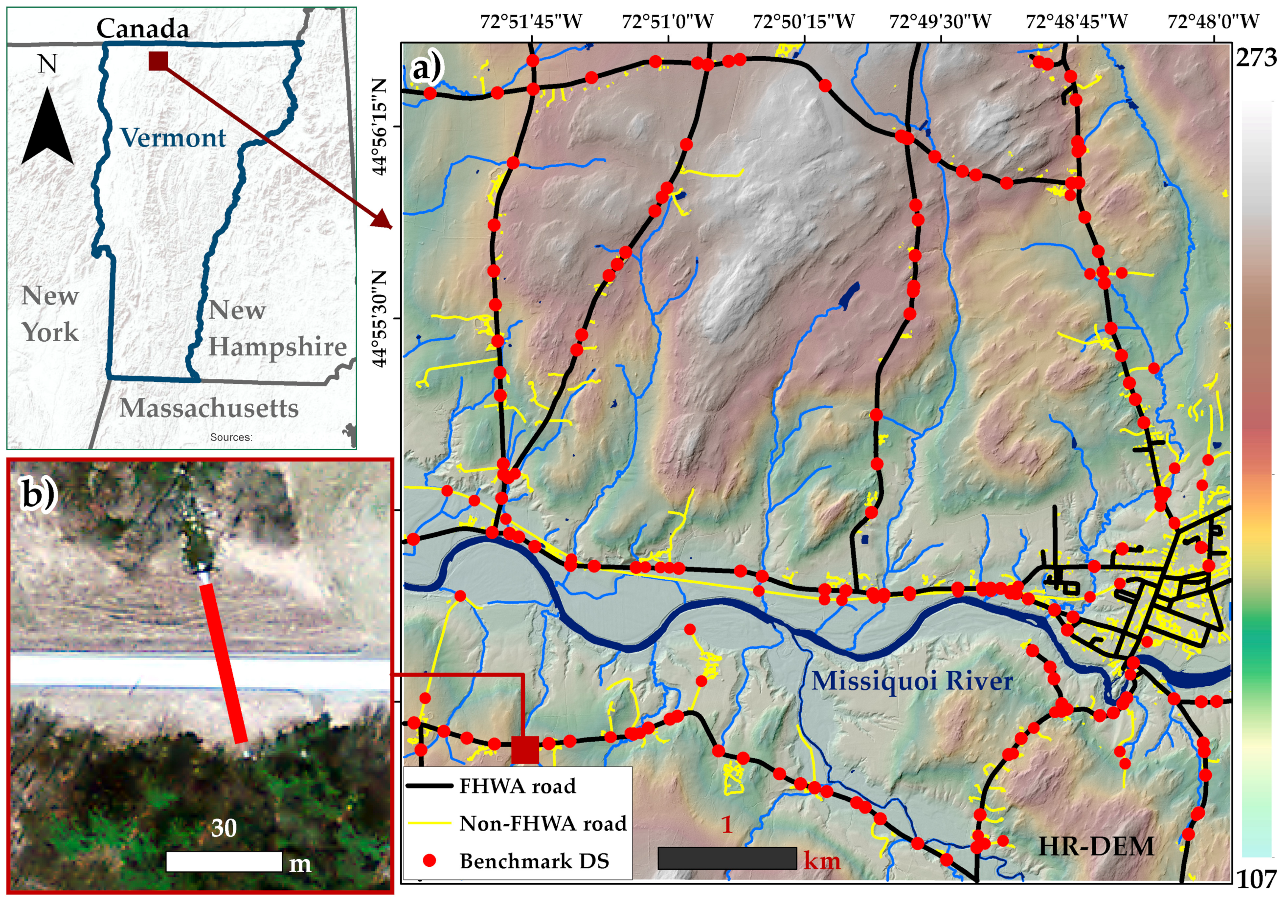
2. Study Area and Datasets
2.1. Study Area and ALS Survey
2.2. Benchmark DS Dataset Along with FHWA and Non-FHWA Roads
3. Methods
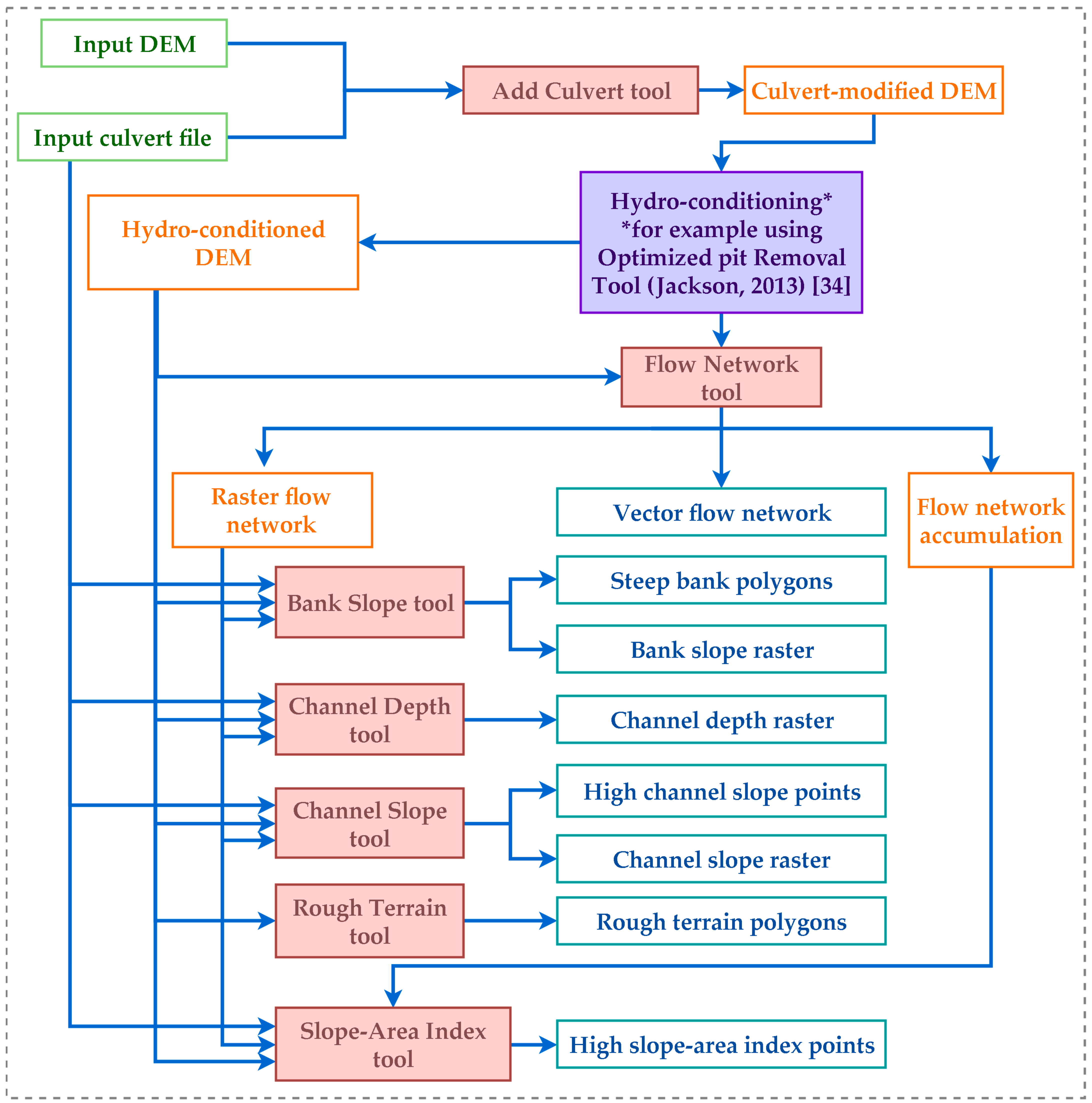
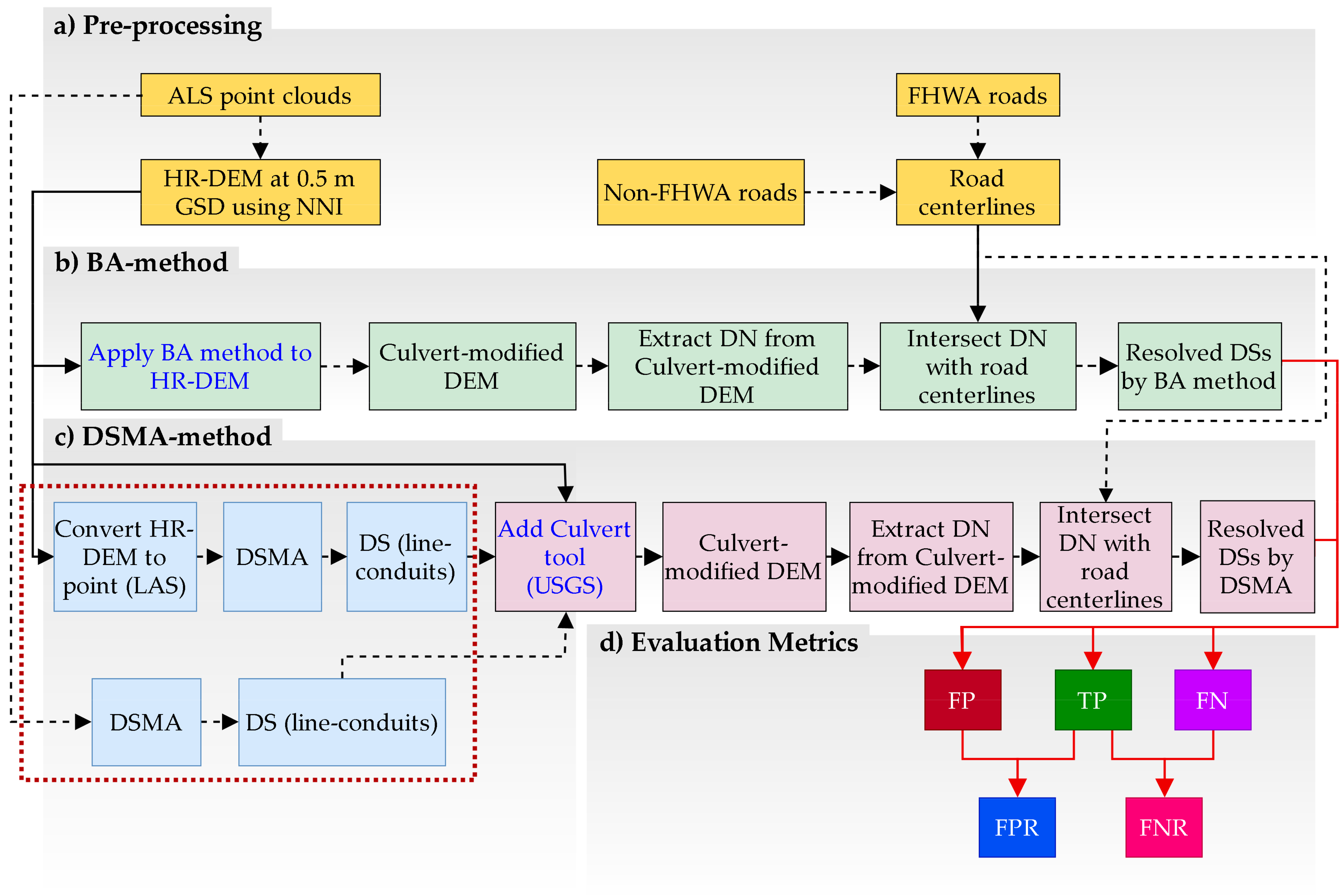
3.1. Preprocessing
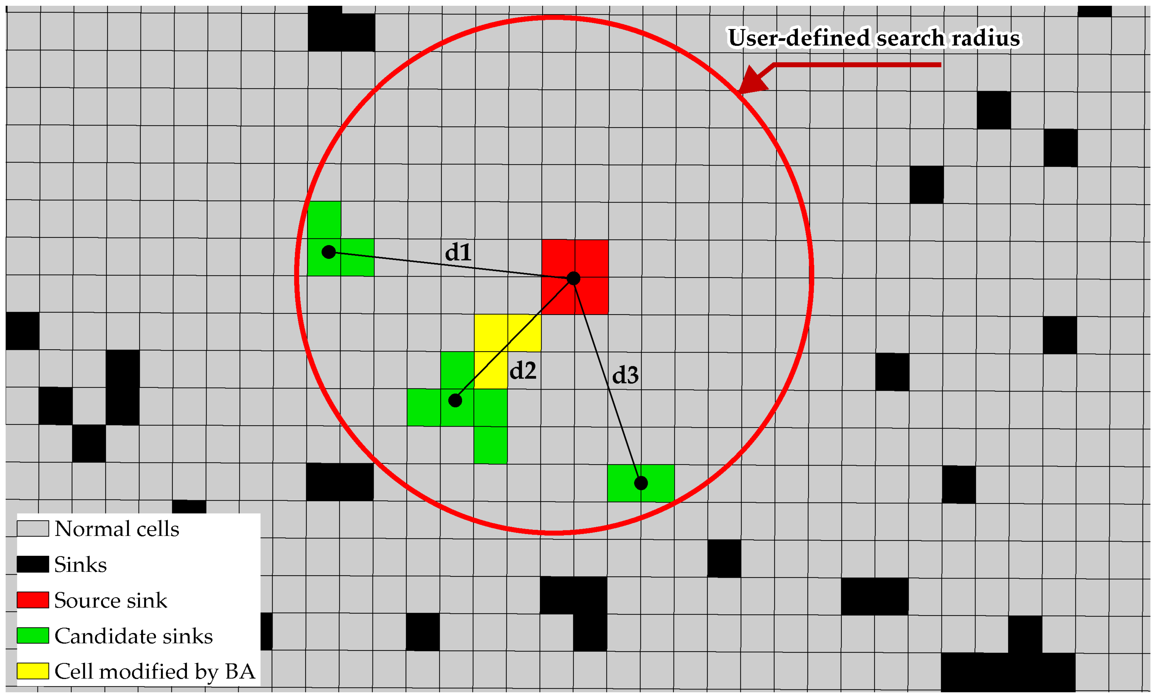
3.2. Breaching Algorithm (BA) Method
3.3. DS Mapping Algorithm (DSMA) Method
3.4. Evaluation Metrics
4. Results
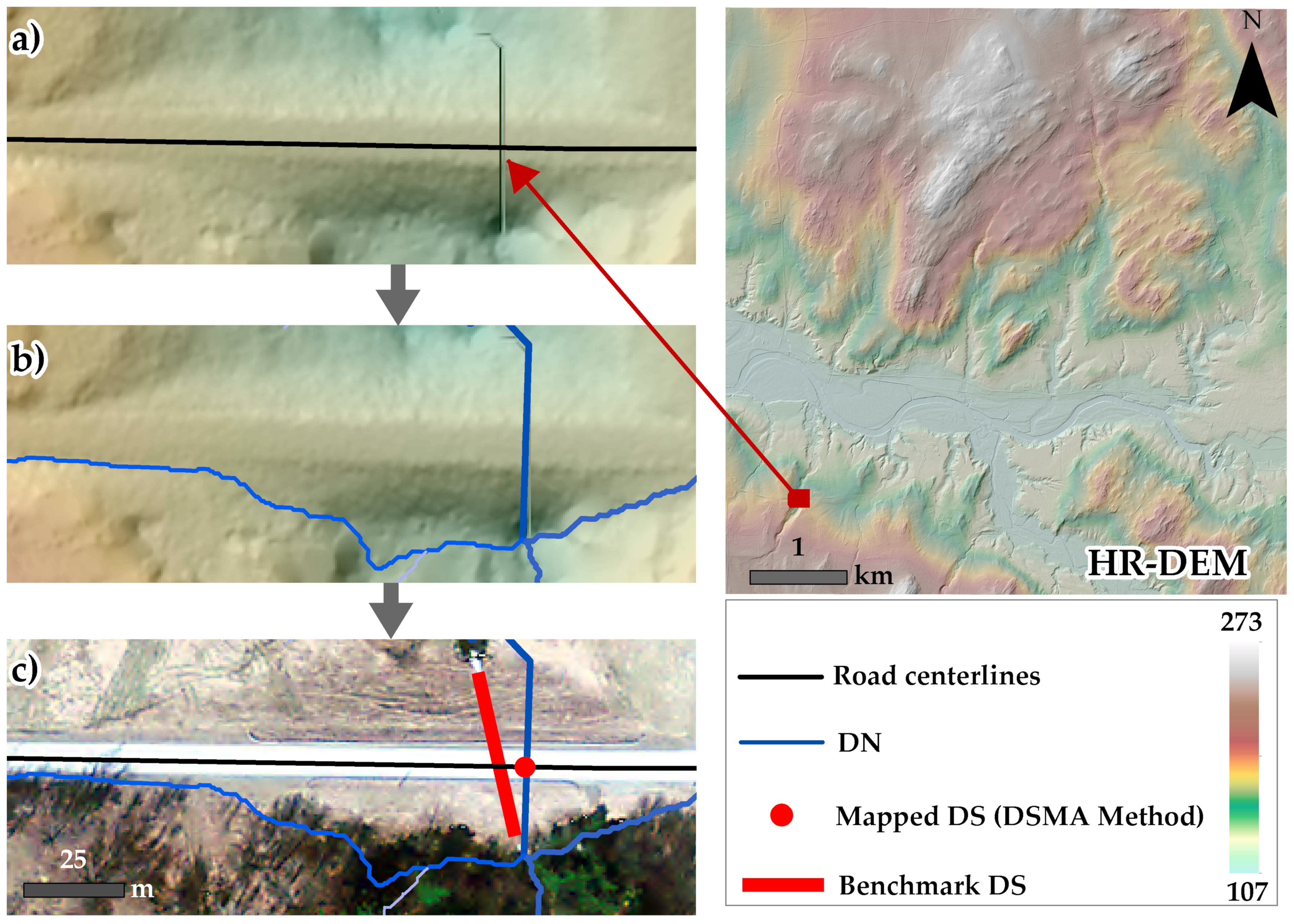
4.1. DS Mapping Assessment of the BA Method Using the HR-DEM
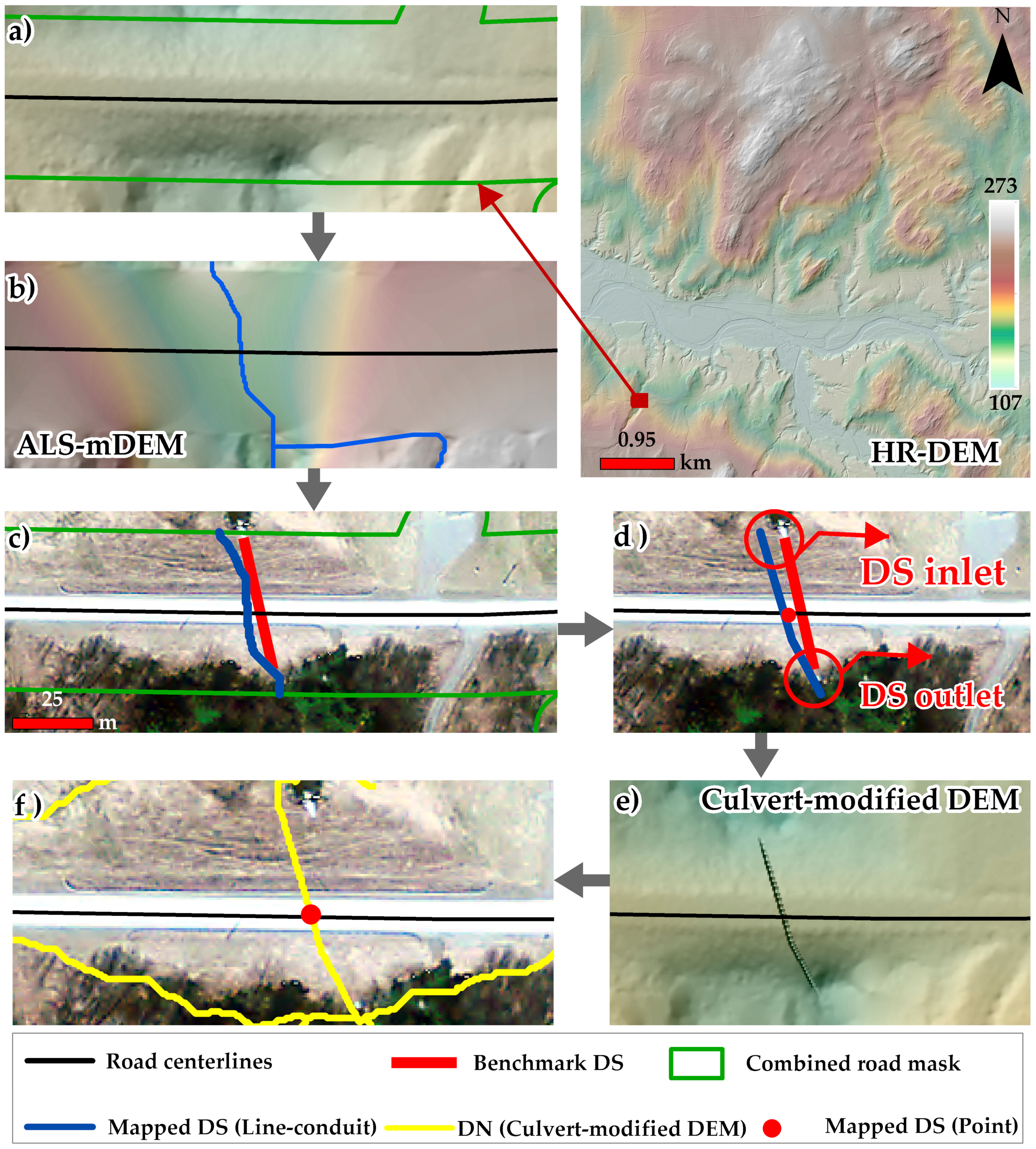
4.2. DS Mapping Assessment of the DSMA Method Using an HR-DEM and ALS Point Clouds
4.3. Comparative Assessment of BA and DSMA Methods
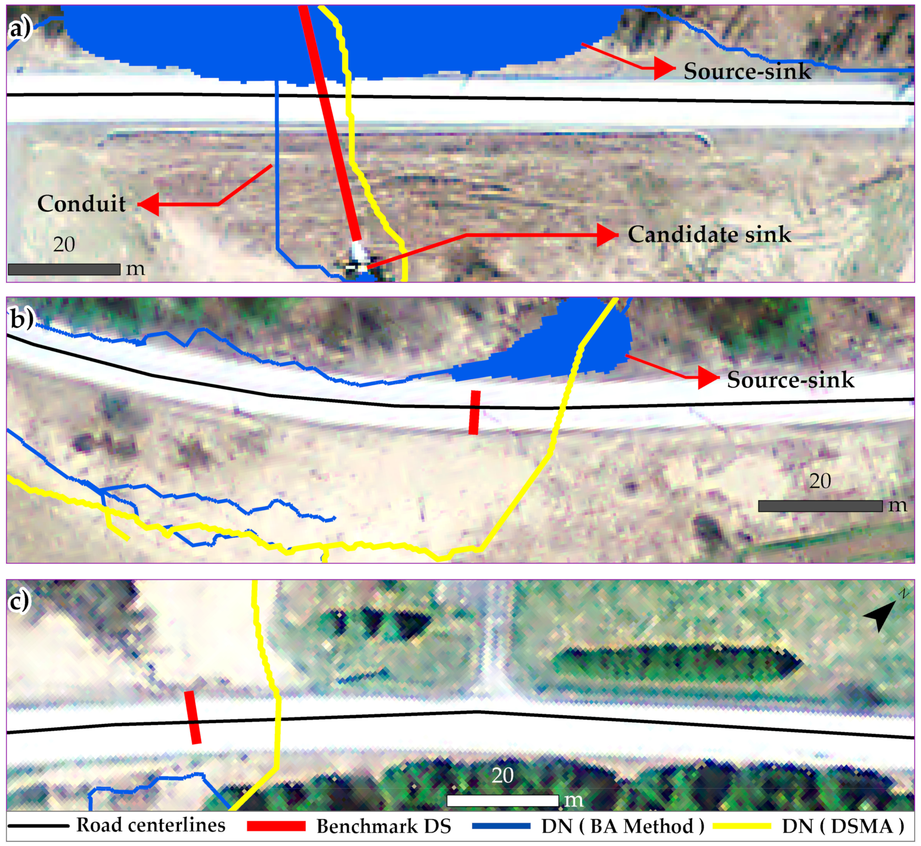
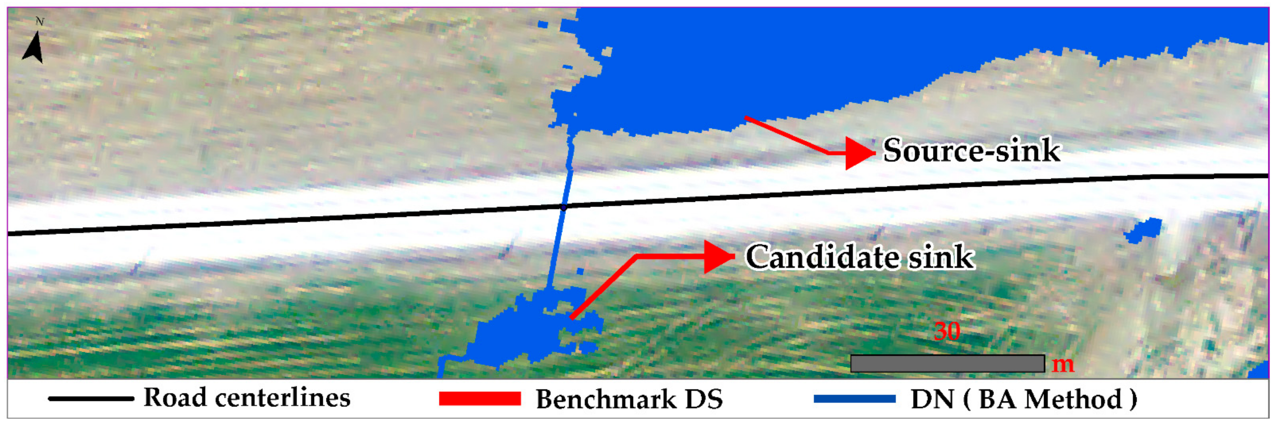
4.3.1. Case-1: No Source or Candidate Sink Found
4.3.2. Case-2: No Solution within the Found Sinks
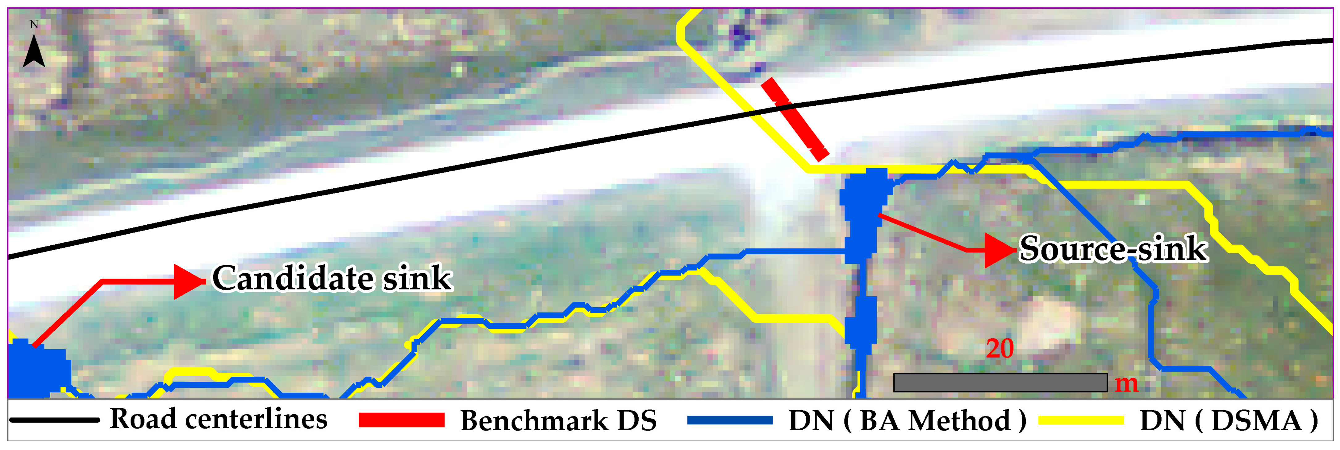
4.3.3. Case-3: Wrong Solutions within the Found Sinks
5. Discussion
6. Conclusions
Author Contributions
Funding
Institutional Review Board Statement
Informed Consent Statement
Data Availability Statement
Acknowledgments
Conflicts of Interest
References
- Martin, R.; Bernhard, H.; Michael, V.; Norbert, P. Chapter Eighteen—Digital Terrain Models from Airborne Laser Scanning for the Automatic Extraction of Natural and Anthropogenic Linear Structures. In Developments in Earth Surface Processes; Smith, M.J., Paron, P., Griffiths, J.S., Eds.; Elsevier: Amsterdam, The Netherlands, 2011; Volume 15, pp. 475–488. [Google Scholar]
- Soilán, M.; Truong-Hong, L.; Riveiro, B.; Laefer, D. Automatic extraction of road features in urban environments using dense ALS data. Int. J. Appl. Earth Obs. Geoinf. 2018, 64, 226–236. [Google Scholar] [CrossRef]
- Ma, H.; Zhou, W.; Zhang, L. DEM refinement by low vegetation removal based on the combination of full waveform data and progressive TIN densification. ISPRS J. Photogramm. Remote Sens. 2018, 146, 260–271. [Google Scholar] [CrossRef]
- Lee, C.-C.; Wang, C.-K. Effect of flying altitude and pulse repetition frequency on laser scanner penetration rate for digital elevation model generation in a tropical forest. GIScience Remote Sens. 2018, 55, 817–838. [Google Scholar] [CrossRef]
- Shi, W.; Deng, S.; Xu, W. Extraction of multi-scale landslide morphological features based on local Gi* using airborne LiDAR-derived DEM. Geomorphology 2018, 303, 229–242. [Google Scholar] [CrossRef]
- Polat, N.; Uysal, M.; Toprak, A.S. An investigation of DEM generation process based on LiDAR data filtering, decimation, and interpolation methods for an urban area. Measurement 2015, 75, 50–56. [Google Scholar] [CrossRef]
- Yang, P.; Ames, D.P.; Fonseca, A.; Anderson, D.; Shrestha, R.; Glenn, N.F.; Cao, Y. What is the effect of LiDAR-derived DEM resolution on large-scale watershed model results? Environ. Model. Softw. 2014, 58, 48–57. [Google Scholar] [CrossRef]
- Archuleta, C.-A.M.; Constance, E.W.; Arundel, S.T.; Lowe, A.J.; Mantey, K.S.; Phillips, L.A. The National Map Seamless Digital Elevation Model Specifications; 11-B9; US Geological Survey: Reston, VA, USA, 2017. [Google Scholar]
- Schumann, G.J.-P.; Bates, P. The Need for a High-Accuracy, Open-Access Global Digital Elevation Model; Frontiers Media SA: Lausanne, Switzerland, 2020. [Google Scholar]
- Poppenga, S.K.; Worstell, B.B. Hydrologic Connectivity: Quantitative Assessments of Hydrologic-Enforced Drainage Structures in an Elevation Model. J. Coast. Res. 2016, 76, 90–106. [Google Scholar] [CrossRef] [Green Version]
- Szypuła, B. Quality assessment of DEM derived from topographic maps for geomorphometric purposes. Open Geosci. 2019, 11, 843–865. [Google Scholar] [CrossRef]
- Cartwright, J.M.; Diehl, T.H. Automated Identification of Stream-Channel Geomorphic Features from High-Resolution Digital Elevation Models in West Tennessee Watersheds; 2328-0328; US Geological Survey: Reston, VA, USA, 2017. [Google Scholar]
- Heidemann, H.K. Lidar Base Specification; 11-B4; US Geological Survey: Reston, VA, USA, 2012; p. 114. [Google Scholar]
- Wang, C.-K.; Fareed, N. Mapping Drainage Structures Using Airborne Laser Scanning by Incorporating Road Centerline Information. Remote Sens. 2021, 13, 463. [Google Scholar] [CrossRef]
- Arendt, R.; Faulstich, L.; Jüpner, R.; Assmann, A.; Lengricht, J.; Kavishe, F.; Schulte, A. GNSS mobile road dam surveying for TanDEM-X correction to improve the database for floodwater modeling in northern Namibia. Environ. Earth Sci. 2020, 79, 1–15. [Google Scholar] [CrossRef]
- Li, R.P.; Tang, Z.H.; Li, X.; Winter, J. Drainage Structure Datasets and Effects on LiDAR-Derived Surface Flow Modeling. ISPRS Int. J. Geo-Inf. 2013, 2, 1136–1152. [Google Scholar] [CrossRef]
- Poppenga, S.K.; Gesch, D.B.; Worstell, B.B. Hydrography change detection: The usefulness of surface channels derived From LiDAR DEMs for updating mapped hydrography. J. Am. Water Resour. Assoc. 2013, 49, 371–389. [Google Scholar] [CrossRef]
- Meegoda, J.N.; Juliano, T.M.; Tang, C. Culvert Information Management System. Transp. Res. Rec. 2009, 2108, 3–12. [Google Scholar] [CrossRef]
- Ewaskiw, A. Culvert Installment and Removals, How They Affect Surrounding Habitat and How We Can Improve Our Methods of Maintenance. Ph.D. Thesis, Lakehead University, Thunder Bay, ON, Canada, 2018. [Google Scholar]
- Salem, O.; Salman, B.; Najafi, M. Culvert asset management practices and deterioration modeling. Transp. Res. Rec. 2012, 2285, 1–7. [Google Scholar] [CrossRef] [Green Version]
- Park, D.; Sullivan, M.; Bayne, E.; Scrimgeour, G. Landscape-level stream fragmentation caused by hanging culverts along roads in Alberta′s boreal forest. Can. J. For. Res. 2008, 38, 566–575. [Google Scholar] [CrossRef]
- Perrin, J., Jr.; Jhaveri, C.S. The economic costs of culvert failures. In Proceedings of the Prepared for TRB 2004 Annual Meeting, Washington, DC, USA, 11–13 July 2004. [Google Scholar]
- Gassman, S.L.; Sasanakul, I.; Pierce, C.E.; Gheibi, E.; Starcher, R.; Ovalle, W.; Rahman, M. Failures of pipe culverts from a 1000-year rainfall event in South Carolina. In Geotechnical Frontiers 2017; American Society of Civil Engineers: Reston, VA, USA, 2017; pp. 114–124. [Google Scholar]
- Najafi, M. An Asset Management Approach for Drainage Infrastructure and Culverts; Midwest Regional University Transportation Center, University of Wisconsin: Madison, WI, USA, 2008. [Google Scholar]
- Perrin, J., Jr.; Dwivedi, R. Need for culvert asset management. Transp. Res. Rec. 2006, 1957, 8–15. [Google Scholar] [CrossRef]
- Venner, M.; Berger, L. Culvert Management Case Studies: Vermont, Oregon, Ohio and Los Angeles County; Federal Highway Administration: Washington, DC, USA, 2014. [Google Scholar]
- Balali, V.; Rad, A.A.; Golparvar-Fard, M. Detection, classification, and mapping of US traffic signs using google street view images for roadway inventory management. Vis. Eng. 2015, 3, 15. [Google Scholar] [CrossRef] [Green Version]
- She, T.; Aouad, G.; Sarshar, M. A geographic information system (GIS)–based bridge management system. Comput. Aided Civ. Infrastruct. Eng. 1999, 14, 417–427. [Google Scholar] [CrossRef]
- Xiong, D.; Floyd, R. Highway Feature and Characteristics Database Development Using Commercial Remote Sensing Technologies, Combined with Mobile Mapping, GIS and GPS; Oak Ridge National Laboratory: Oak Ridge, TN, USA, 2004. [Google Scholar]
- Sabatini, R.; Richardson, M.A.; Gardi, A.; Ramasamy, S. Airborne laser sensors and integrated systems. Prog. Aerosp. Sci. 2015, 79, 15–63. [Google Scholar] [CrossRef]
- Eitel, J.U.H.; Höfle, B.; Vierling, L.A.; Abellán, A.; Asner, G.P.; Deems, J.S.; Glennie, C.L.; Joerg, P.C.; LeWinter, A.L.; Magney, T.S.; et al. Beyond 3-D: The new spectrum of lidar applications for earth and ecological sciences. Remote Sens. Environ. 2016, 186, 372–392. [Google Scholar] [CrossRef] [Green Version]
- Biron, P.M.; Choné, G.; Buffin-Bélanger, T.; Demers, S.; Olsen, T. Improvement of streams hydro-geomorphological assessment using LiDAR DEMs. Earth Surf. Process. Landf. 2013, 38, 1808–1821. [Google Scholar] [CrossRef]
- Vocal Ferencevic, M.; Ashmore, P. Creating and evaluating digital elevation model-based stream-power map as a stream assessment tool. River Res. Appl. 2012, 28, 1394–1416. [Google Scholar] [CrossRef]
- Jackson, S. Optimized Pit Removal V1. 5.1 Tutorial. Center for Research in Water Resources University of Texas at Austin. Available online: http://tools.crwr.utexas.edu/OptimizedPitRemoval/CRWR%20Tools%20Optimized%20Pit%20Removal.html (accessed on 6 February 2013).
- Poppenga, S.K.; Worstell, B.B.; Stoker, J.M.; Greenlee, S.K. Using Selective Drainage Methods to Extract Continuous Surface Flow from 1-Meter Lidar-Derived Digital Elevation Data; US Geological Survey: Reston, VA, USA, 2010. [Google Scholar]
- Lindsay, J.B. The practice of DEM stream burning revisited. Earth Surface Process. Landf. 2016, 41, 658–668. [Google Scholar] [CrossRef]
- Lidberg, W.; Nilsson, M.; Lundmark, T.; Ågren, A.M. Evaluating preprocessing methods of digital elevation models for hydrological modelling. Hydrol. Process. 2017, 31, 4660–4668. [Google Scholar] [CrossRef] [Green Version]
- Lindsay, J.B.; Dhun, K. Modelling surface drainage patterns in altered landscapes using LiDAR. Int. J. Geogr. Inf. Sci. 2015, 29, 397–411. [Google Scholar] [CrossRef]
- White, B.; Ogilvie, J.; Campbell, D.M.; Hiltz, D.; Gauthier, B.; Chisholm, H.K.H.; Wen, H.K.; Murphy, P.N.; Arp, P.A. Using the cartographic depth-to-water index to locate small streams and associated wet areas across landscapes. Can. Water Resour. J. Rev. Can. Ressour. Hydr. 2012, 37, 333–347. [Google Scholar] [CrossRef]
- MacFaden, S. LandLandcov_NFLLAKELCLU. Available online: http://maps.vcgi.vermont.gov/gisdata/metadata/LandLandcov_NFLLAKELCLU.xml (accessed on 6 February 2021).
- Stoker, J.; Harding, D.; Parrish, J. ed for a National Lidar Dataset. Photogramm. Eng. Remote Sens. 2008, 74, 1067. [Google Scholar]
- Crosby, C.J.; Arrowsmith, J.R.; Nandigam, V. Chapter 11—Zero to a trillion: Advancing Earth surface process studies with open access to high-resolution topography. In Developments in Earth Surface Processes; Tarolli, P., Mudd, S.M., Eds.; Elsevier: Amsterdam, The Netherlands, 2020; Volume 23, pp. 317–338. [Google Scholar]
- Krishnan, S.; Crosby, C.; Nandigam, V.; Phan, M.; Cowart, C.; Baru, C.; Arrowsmith, R. OpenTopography: A services oriented architecture for community access to LIDAR topography. In Proceedings of the 2nd International Conference on Computing for Geospatial Research & Applications, Washington, DC, USA, 23–25 May 2011; pp. 1–8. [Google Scholar]
- O’Neil-Dunne, J. Mapping Impervious Surfaces in the Lake Champlain Basin; Lake Champlain Basin Program Final Report, Technical Report No 76; Lake Champlain Basin Program: Grand Isle, VT, USA, 2013. [Google Scholar]
- Commissions, V.R.P. TransStructures_BCVOBCIT. Available online: https://vtculverts.org/structures (accessed on 2 February 2021).
- Anguelov, D.; Dulong, C.; Filip, D.; Frueh, C.; Lafon, S.; Lyon, R.; Ogale, A.; Vincent, L.; Weaver, J. Google street view: Capturing the world at street level. Computer 2010, 43, 32–38. [Google Scholar] [CrossRef]
- Woodrow, K.; Lindsay, J.B.; Berg, A.A. Evaluating DEM conditioning techniques, elevation source data, and grid resolution for field-scale hydrological parameter extraction. J. Hydrol. 2016, 540, 1022–1029. [Google Scholar] [CrossRef]
- Verdin, K.L.; Jenson, S. Development of continental scale DEMs and extraction of hydrographic features. In Proceedings of the Third International Conference/Workshop on Integrating GIS and Environmental Modeling, Santa Fe, NM, USA, 21–26 January 1996; pp. 1–12. [Google Scholar]
- Lindsay, J.B. Whitebox GAT: A case study in geomorphometric analysis. Comput. Geosci. 2016, 95, 75–84. [Google Scholar] [CrossRef]
- Duke, G.D.; Kienzle, S.W.; Johnson, D.L.; Byrne, J.M. Improving overland flow routing by incorporating ancillary road data into digital elevation models. J. Spat. Hydrol. 2003, 3, 23–49. [Google Scholar]
- Bettinger, P.; Merry, K.; Boston, K. (Eds.) Chapter 7—Map Development and Generalization. In Mapping Human and Natural Systems; Academic Press: Cambridge, MA, USA, 2020; pp. 255–281. [Google Scholar] [CrossRef]
- Duke, G.D.; Kienzle, S.W.; Johnson, D.L.; Byrne, J.M. Incorporating ancillary data to refine anthropogenically modified overland flow paths. Hydrol. Process. 2006, 20, 1827–1843. [Google Scholar] [CrossRef]
- He, Y.; Song, Z.; Liu, Z. Updating highway asset inventory using airborne LiDAR. Measurement 2017, 104, 132–141. [Google Scholar] [CrossRef]
- Persendt, F.C.; Gomez, C. Assessment of drainage network extractions in a low-relief area of the Cuvelai Basin (Namibia) from multiple sources: LiDAR, topographic maps, and digital aerial orthophotographs. Geomorphology 2016, 260, 32–50. [Google Scholar] [CrossRef] [Green Version]
- Amatya, D.; Trettin, C.; Panda, S.; Ssegane, H. Application of LiDAR data for hydrologic assessments of low-gradient coastal watershed drainage characteristics. J. Geogr. Inf. Syst. 2013, 5, 175–191. [Google Scholar] [CrossRef] [Green Version]


| Road Type | FPR | FNR | |||||
|---|---|---|---|---|---|---|---|
| Case-1 | Case-2 | Case-3 | |||||
| BA Method | FHWA roads | 78 | 23 | 13 | 31 | 0.28 | 0.32 |
| Non-FHWA roads | 16 | 19 | 6 | 25 | 0.62 | 0.61 | |
| Road Type | FPR | FNR | ||||
|---|---|---|---|---|---|---|
| DSMA Method (HR-DEM) | FHWA roads | 108 | 6 | 9 | 0.05 | 0.07 |
| Non-FHWA roads | 27 | 15 | 4 | 0.12 | 0.38 | |
| DSMA Method (ALS ground clouds) | FHWA roads | 108 | 6 | 9 | 0.05 | 0.07 |
| Non-FHWA roads | 27 | 15 | 4 | 0.12 | 0.38 |
| Min | First Quartile | Median | Third Quartile | Max | Mean | |
|---|---|---|---|---|---|---|
| Study area (36 km2) | 0.65 | 5.71 | 10.17 | 10.17 | 72.53 | 15.82 |
Publisher’s Note: MDPI stays neutral with regard to jurisdictional claims in published maps and institutional affiliations. |
© 2021 by the authors. Licensee MDPI, Basel, Switzerland. This article is an open access article distributed under the terms and conditions of the Creative Commons Attribution (CC BY) license (https://creativecommons.org/licenses/by/4.0/).
Share and Cite
Fareed, N.; Wang, C.-K. Accuracy Comparison on Culvert-Modified Digital Elevation Models of DSMA and BA Methods Using ALS Point Clouds. ISPRS Int. J. Geo-Inf. 2021, 10, 254. https://0-doi-org.brum.beds.ac.uk/10.3390/ijgi10040254
Fareed N, Wang C-K. Accuracy Comparison on Culvert-Modified Digital Elevation Models of DSMA and BA Methods Using ALS Point Clouds. ISPRS International Journal of Geo-Information. 2021; 10(4):254. https://0-doi-org.brum.beds.ac.uk/10.3390/ijgi10040254
Chicago/Turabian StyleFareed, Nadeem, and Chi-Kuei Wang. 2021. "Accuracy Comparison on Culvert-Modified Digital Elevation Models of DSMA and BA Methods Using ALS Point Clouds" ISPRS International Journal of Geo-Information 10, no. 4: 254. https://0-doi-org.brum.beds.ac.uk/10.3390/ijgi10040254