
Spatial Allocation Based on Physiological Needs and Land Suitability Using the Combination of Ecological Footprint and SVM (Case Study: Java Island, Indonesia)

 ,
, 
Abstract
:1. Introduction
2. Materials and Methods
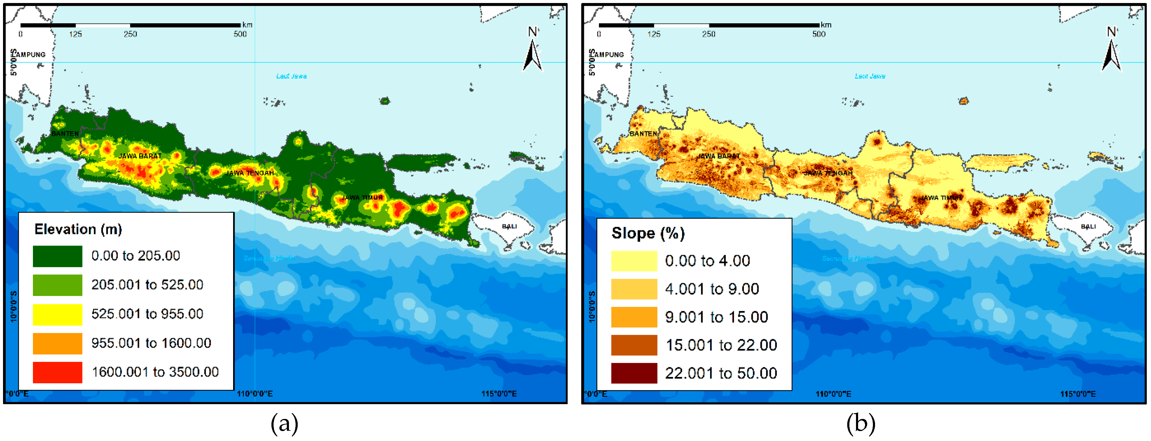
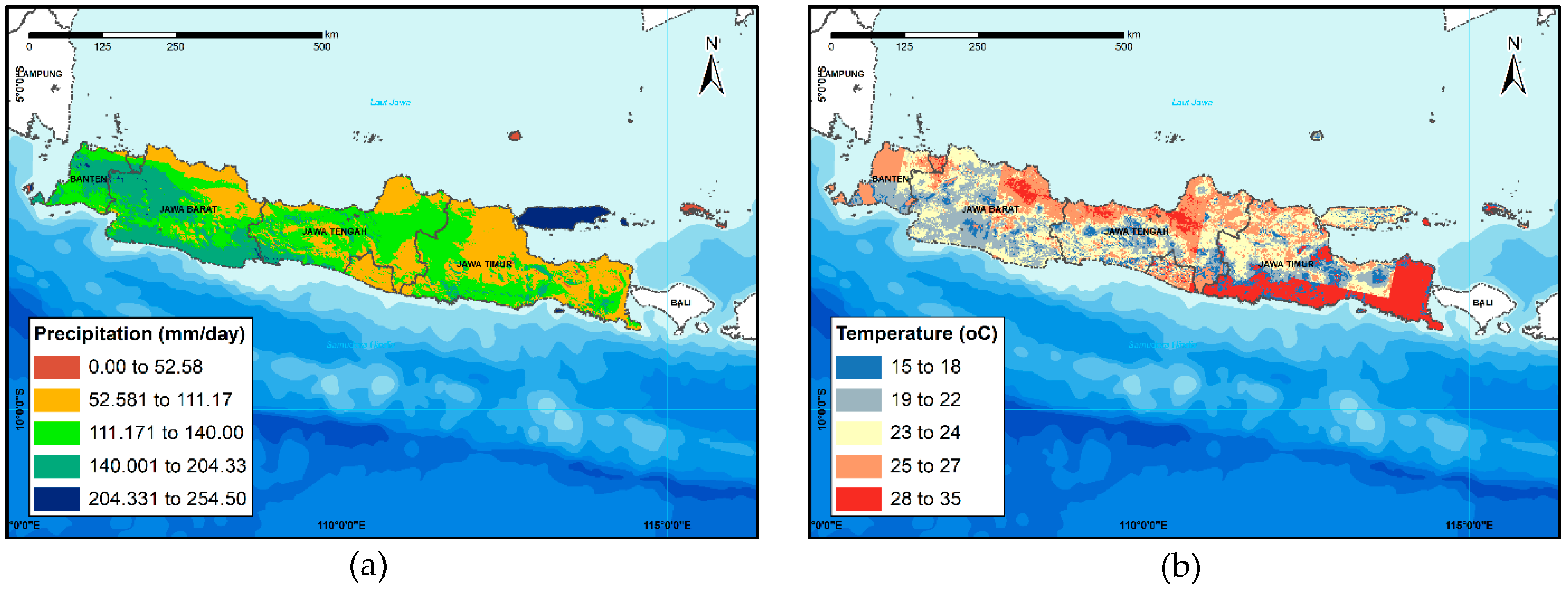
2.1. Materials
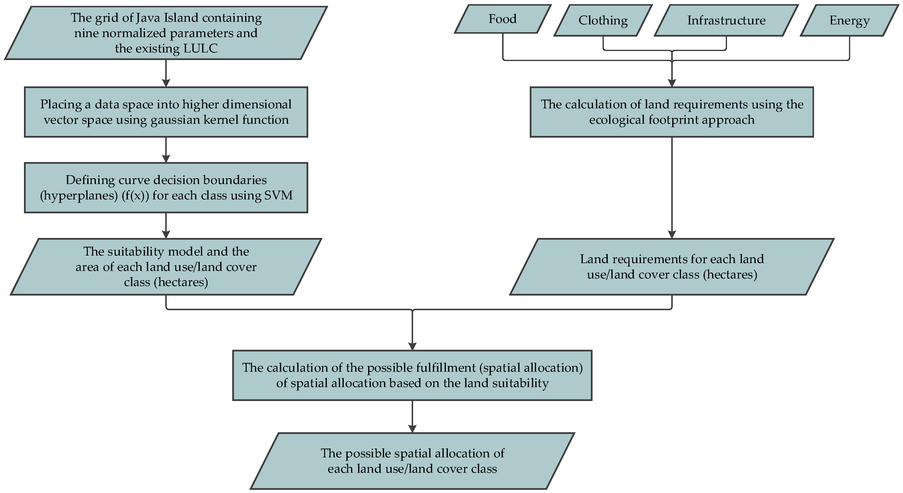
2.2. Methods
- Perform the calculation of land use/land cover spatial allocation based on physiological needs using an ecological footprint approach with land use/land cover data and statistical data. The spatial allocation can also be carried out using several scenarios of meeting the needs.
- Conduct land suitability analysis using the SVM with kernel trick. There are nine parameters and several sample points. The number of sample points and the sampling method refer to the standards set for geospatial information, namely SNI ISO 19157.
2.2.2. The Calculation of Spatial Allocation with the Ecological Footprint (EF) Approach
| = | ecological footprint or land requirements (gm2); | |
| = | number of basic human needs (kg); | |
| = | ||
| = | footprint intensity (m2/kg); | |
| = | yield factor (wm2/m2); | |
| = | equivalence factor (gm2/wm2). |
2.2.3. Land Suitability Model with Support Vector Machine (SVM)
3. Results
3.1. Spatial Allocation Based on Physiological Needs Using Ecological Footprint (EF)
- Indonesia’s food sector is grouped into eight categories: grains, tubers, animal food, oils and fats, oily fruits/seeds, nuts, sugar, and vegetables and fruit [72,73]. The food sector is produced from wetland agriculture, dryland agriculture, and plantations. The calculation results of the ecological footprint per person for the food sector can be seen in Table 4.
- The clothing/textile sector is produced with raw materials from natural fibers and synthetic fibers [74,75]. The raw material for textiles in Indonesia, which uses natural fibers (cotton), reaches 42%, and the rest is produced from synthetic fibers [76,77]. Therefore, the raw material for clothing/textiles taken into account in this model is cotton made from plantation land. The calculation results of the ecological footprint per person for the clothing/textile sector can be seen in Table 5.
- The infrastructure sector includes residents’ needs for housing and public spaces classified into built-up land types. Calculation of the required built-up land area uses the standard of space requirements per person [78,79]. Infrastructures that require wood include infrastructure with a physical structure, namely, a residence (house), cultural and recreational facilities, shopping and commercial centers, religious facilities, health facilities, and educational facilities. Therefore, the proportion of wood demand for buildings must be considered in this model (m3 of wood/m2 of buildings). Wood as a building material is produced from forest land. The calculation results of the ecological footprint per person for the infrastructure sector can be seen in Table 6.
- The energy sector involved in modeling includes electricity, gas, and fuel oil. The amount of energy needed per person is the average of the total energy use in Java. Energy use data are obtained from the Electricity Statistics provided by the Ministry of Energy and Mineral Resources of the Republic of Indonesia. The energy sector is produced from built-up land and pastureland. The calculation results of the ecological footprint per person for the energy sector can be seen in Table 7.
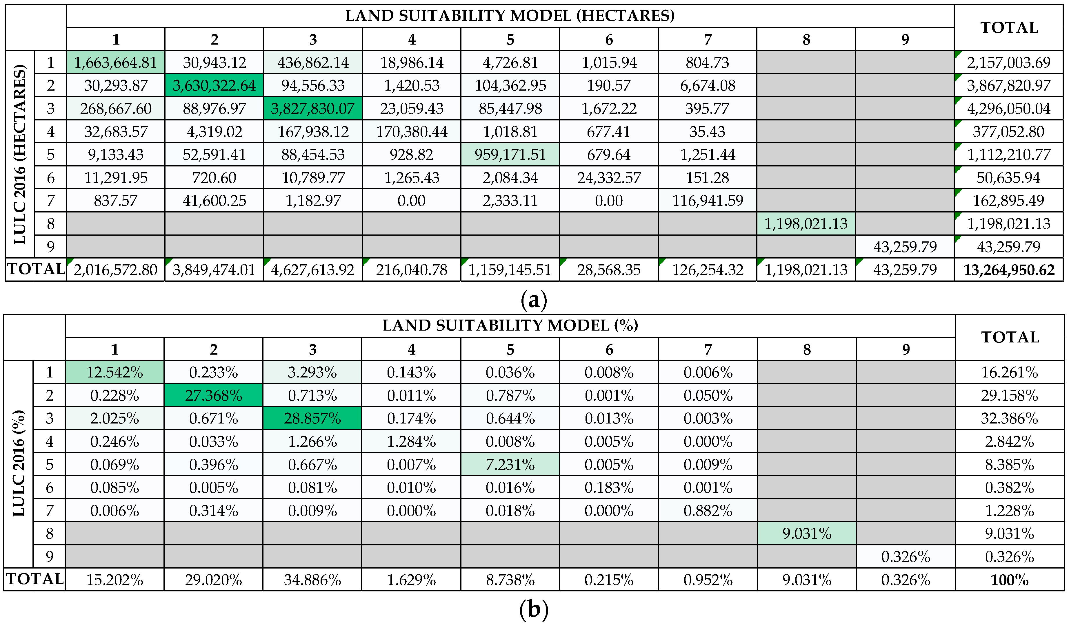
3.2. Land Suitability Classification Using SVM
4. Discussion
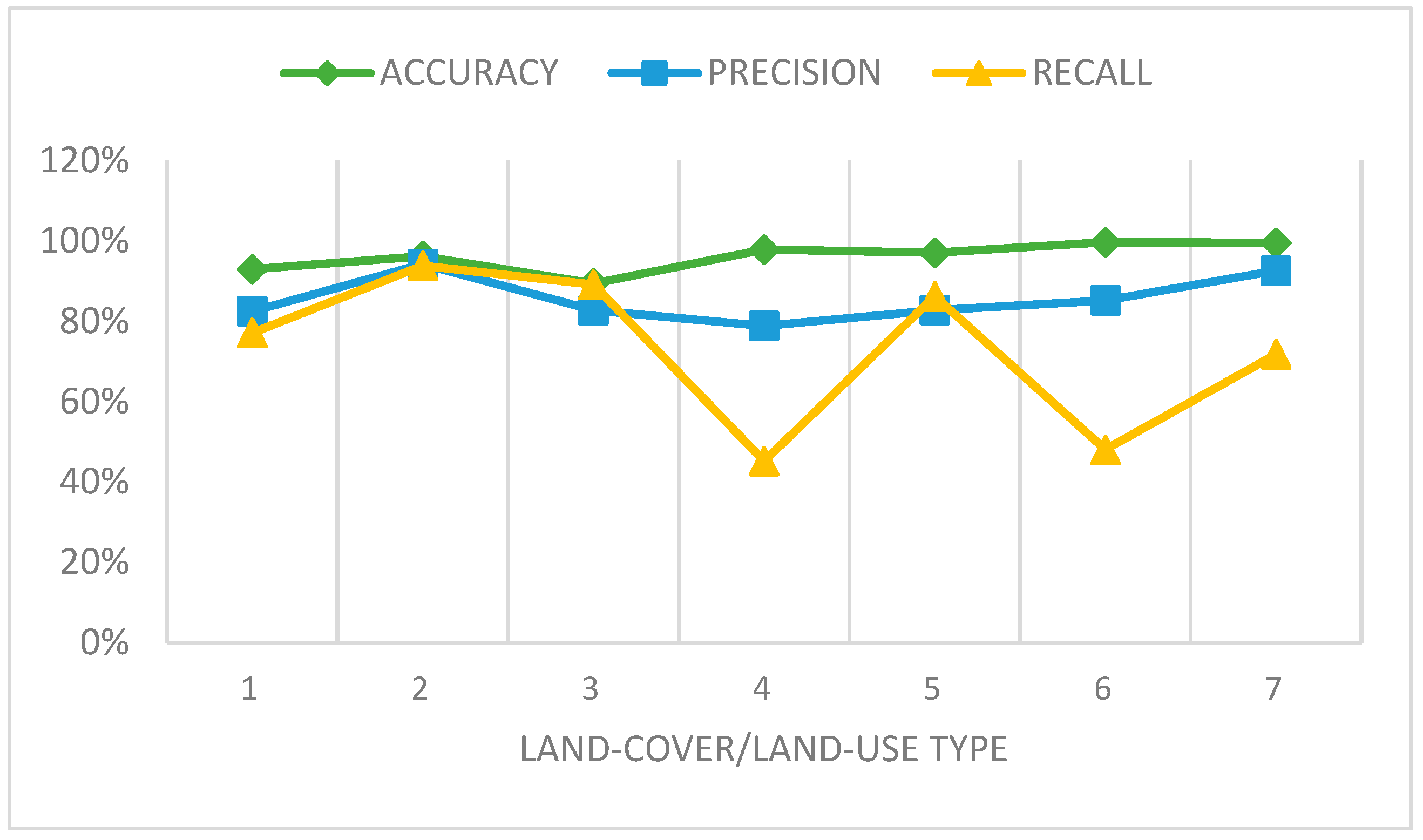
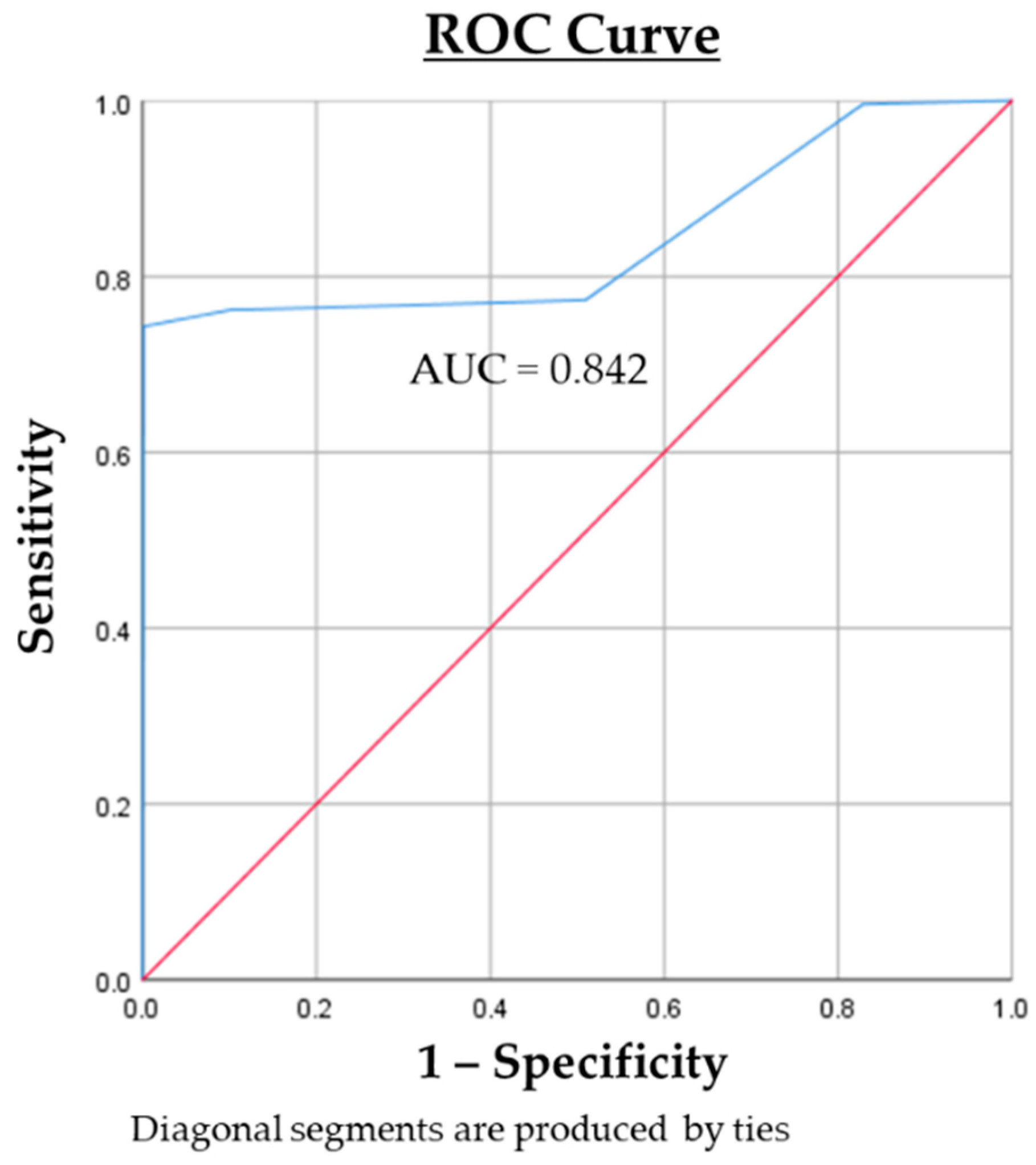
4.1. The Overall Performance of Land Suitability Model in Java Island
4.2. Fulfillment of Spatial Allocation Based on Land Suitability
5. Conclusions
Author Contributions
Funding
Data Availability Statement
Acknowledgments
Conflicts of Interest
References
- Abulof, U. Introduction: Why we need Maslow in the twenty-first century. Society 2017, 54, 508–509. [Google Scholar] [CrossRef] [Green Version]
- Fallatah, R.H.M.; Syed, J. A critical review of Maslow’s hierarchy of needs. In Employee Motivation in Saudi Arabia; Palgrave Macmillan: Cham, Switzerland, 2018; pp. 19–60. [Google Scholar] [CrossRef]
- Lane, M. The Development of a Carrying Capacity Assessment Model for the Australian Socio-Environmental Context. Doctoral Dissertation, Queensland University of Technology, Brisbane, Queensland, Australia, 2014. [Google Scholar]
- Meadows, D.; Randers, J.; Meadows, D. Limits to Growth: The-30-Year Update; Earthscan: London, UK, 2005. [Google Scholar]
- Borucke, M.; Moore, D.; Cranston, G.; Gracey, K.; Iha, K.; Larson, J.; Lazarus, E.; Carlos, J.; Wackernagel, M.; Galli, A. Accounting for demand and supply of the biosphere’s regenerative capacity: The national footprint accounts’ underlying methodology and framework. Ecol. Indic. 2013, 24, 518–533. [Google Scholar] [CrossRef]
- Wackernagel, M.; Lin, D.; Hanscom, L.; Galli, A.; Iha, K. Ecological Footprint. Encycl. Ecol. 2019, 4, 270–282. [Google Scholar] [CrossRef]
- Steffen, W.; Sanderson, R.A.; Tyson, P.D.; Jäger, J.; Matson, P.A.; Moore, B., III; Oldfield, F.; Richardson, K.; Schellnhuber, H.J.; Turner, B.L.; et al. Global Change and the Earth System: A Planet under Pressure, 1st ed.; Springer: Berlin/Heidelberg, Germany, 2005. [Google Scholar] [CrossRef]
- UN Environment; United Nations Environment Programme (UNEP). Global Environment Outlook 5—Environment for the Future We Want; United Nations Environment Programme (UNEP): Nairobi, Kenya, 2012. [Google Scholar]
- Daly, H.E. Toward some operational principles of sustainable development. Ecol. Econ. 1990, 2, 1–6. [Google Scholar] [CrossRef]
- Intergovernmental Panel on Climate Change (IPCC). Climate Change 2014: Synthesis Report. Contribution of Working Groups I, II and III to the Fifth Assessment Report of the Intergovernmental Panel on Climate Change; Pachauri, R.K., Meyer, L.A., Eds.; IPCC: Geneva, Switzerland, 2014. [Google Scholar]
- Mancini, M.S.; Galli, A.; Niccolucci, V.; Lin, D.; Bastianoni, S.; Wackernagel, M.; Marchettini, N. Ecological footprint: Refining the carbon footprint calculation. Ecol. Indic. 2016, 61, 390–403. [Google Scholar] [CrossRef]
- FAO Land and Water Development Division. Planning for Sustainable Use of Land Resources—Towards a New Approach; FAO Land and Water Bulletin: Rome, Italy, 1995; pp. 1–8. [Google Scholar]
- Badan Standardisasi Nasional. Klasifikasi Penutup Lahan—Bagian 1: Skala Kecil Dan Menengah; Badan Standarisasi Nasional: Jakarta, Indonesia, 2014; p. 51. [Google Scholar]
- Di Gregorio, A.; Henry, M.; Donegan, E.; Finegold, Y.; Latham, J.; Jonckheere, I.; Cumani, R. Land Cover Classification System: Classification Concepts—Software Version 3; Food and Agriculture Organization of The United Nations: Rome, Italy, 2016. [Google Scholar]
- Aquilué, N.; de Cáceres, M.; Fortin, M.; Fall, A. A spatial allocation procedure to model land-use/land-cover changes: Accounting for occurrence and spread processes. Ecol. Modell. 2017, 344, 73–86. [Google Scholar] [CrossRef]
- Moser, S.C. A partial instructional module on global and regional land use/cover change: Assessing the data and searching for general relationships. GeoJournal 1996, 39, 241–283. [Google Scholar] [CrossRef]
- Noi, P.T.; Kappas, M. Comparison of random forest, k-nearest neighbor, and support vector machine classifiers for land cover classification using sentinel-2 imagery. Sensors 2018, 18, 18. [Google Scholar] [CrossRef] [Green Version]
- De Alvarenga, R.A.F.; da Silva, V.P., Jr.; Soares, S.R. Comparison of the ecological footprint and a life cycle impact assessment method for a case study on brazilian broiler feed production. J. Clean. Prod. 2012, 28, 25–32. [Google Scholar] [CrossRef]
- Guinee, J.B.; Heijungs, R.; Huppes, G.; Zamagni, A.; Masoni, P.; Buonamici, R.; Ekvall, T.; Rydberg, T. Life cycle assessment: Past, present, and future. Environ. Sci. Technol. 2011, 45, 90–96. [Google Scholar] [CrossRef]
- Miao, C.L.; Sun, L.Y.; Yang, L. The studies of ecological environmental quality assessment in Anhui province based on ecological footprint. Ecol. Indic. 2016, 60, 879–883. [Google Scholar] [CrossRef]
- Gao, J.; Tian, M. Analysis of over-consumption of natural resources and the ecological trade deficit in China based on ecological footprints. Ecol. Indic. 2016, 61, 899–904. [Google Scholar] [CrossRef]
- Hopton, M.E.; White, D. A simplified ecological footprint at a regional scale. J. Environ. Manag. 2012, 111, 279–286. [Google Scholar] [CrossRef]
- Wackernagel, M.; Moran, D.; Goldfinger, S.; Monfreda, C.; Welch, A.; Murray, M.; Burns, S.; Konigel, C.; Peck, J.; King, P.; et al. Europe 2005: The Ecological Footprint; Lyons, J., Ed.; The WWF European Policy Office: Cambridge, UK, 2005. [Google Scholar]
- Galli, A. On the rationale and policy usefulness of ecological footprint accounting: The case of Morocco. Environ. Sci. Policy 2015, 48, 210–224. [Google Scholar] [CrossRef] [Green Version]
- Lin, D.; Hanscom, L.; Martindill, J.; Borucke, M.; Cohen, L.; Galli, A.; Lazarus, E.; Zokai, G.; Iha, K.; Wackernagel, M. Working Guidebook to the National Footprint Accounts; Global Footprint Network: Oakland, CA, USA, 2018. [Google Scholar]
- Zhao, J.; Ma, C.; Zhao, X.; Wang, X. Spatio-temporal dynamic analysis of sustainable development in China based on the footprint family. Int. J. Environ. Res. Public Health 2018, 15, 246. [Google Scholar] [CrossRef] [Green Version]
- Yin, Y.; Han, X.; Wu, S. Spatial and temporal variations in the ecological footprints in northwest China from 2005 to 2014. Sustainability 2017, 9, 597. [Google Scholar] [CrossRef] [Green Version]
- Wang, Y.; Jiang, Y.; Zheng, Y.; Wang, H. Assessing the ecological carrying capacity based on revised three-dimensional ecological footprint model in inner Mongolia, China. Sustainability 2019, 11, 2002. [Google Scholar] [CrossRef] [Green Version]
- Lu, Y.; Li, X.; Ni, H.; Chen, X.; Xia, C.; Jiang, D.; Fan, H. Temporal-spatial evolution of the urban ecological footprint based on net primary productivity: A case study of Xuzhou Central Area, China. Sustainability 2019, 11, 199. [Google Scholar] [CrossRef] [Green Version]
- Wu, D.; Liu, J. Spatial and temporal evaluation of ecological footprint intensity of Jiangsu Province at the county-level scale. Int. J. Environ. Res. Public Health 2020, 17, 7833. [Google Scholar] [CrossRef] [PubMed]
- Wackernagel, M.; Cranston, G.; Morales, J.C.; Galli, A. Ecological footprint accounts: Criticisms and applications. In Handbook of Sustainable Development, 2nd ed.; Atkinson, G., Dietz, S., Neumayer, E., Agarwala, M., Eds.; Edward Elgar Publishing: Cheltenham, UK, 2014; pp. 371–396. [Google Scholar] [CrossRef]
- Erb, K. Actual land demand of austria 1926–2000: A variation on ecological footprint assessments. Land Use Policy 2004, 21, 247–259. [Google Scholar] [CrossRef]
- Bicknell, K.B.; Ball, R.J.; Cullen, R.; Bigsby, H.R. New methodology for the ecological footprint with an application to the New Zealand economy. Ecol. Econ. 1998, 27, 149–160. [Google Scholar] [CrossRef] [Green Version]
- Chengkang, G.; Dahe, J.; Dan, W.; Jonathan, Y. Calculation of ecological footprint based on modified method and quantitative analysis of its impact factors—A case study of Shanghai. Chin. Geogr. Sci. 2006, 16, 306–313. [Google Scholar] [CrossRef]
- Haberl, H.; Erb, K.; Krausmann, F. How to calculate and interpret ecological footprints for long periods of time: The case of Austria 1926–1995. Ecol. Econ. 2001, 38, 25–45. [Google Scholar] [CrossRef]
- Hubacek, K.; Giljum, S. Applying physical input-output analysis to estimate land appropriation (ecological footprints) of international trade activities. Ecol. Econ. 2003, 44, 137–151. [Google Scholar] [CrossRef]
- van Vuuren, D.P.; Bouwman, L.F. Exploring past and future changes in the ecological footprint for world regions. Ecol. Econ. 2005, 52, 43–62. [Google Scholar] [CrossRef]
- Lane, M.; Dawes, L.; Grace, P. Scalar considerations in carrying capacity assessment: An Australian example. Popul. Environ. 2014, 36, 356–371. [Google Scholar] [CrossRef] [Green Version]
- Lane, M.; Dawes, L.; Grace, P. The essential parameters of a resource-based carrying capacity assessment model: An Australian case study. Ecol. Modell. 2014, 272, 220–231. [Google Scholar] [CrossRef] [Green Version]
- IUCN; UNEP; WWF. Caring for the Earth: A Strategy for Sustainable Living; Munro, D.A., Holdgate, M.W., Eds.; Earthscan: Gland, Switzerland, 1991. [Google Scholar]
- McDowell, R.W.; Snelder, T.; Harris, S.; Lilburne, L.; Larned, S.T.; Scarsbrook, M.; Curtis, A.; Holgate, B.; Phillips, J.; Taylor, K. The land use suitability concept: Introduction and an application of the concept to inform sustainable productivity within environmental constraints. Ecol. Indic. 2018, 91, 212–219. [Google Scholar] [CrossRef]
- Hopkins, L.D. Methods for generating land suitability maps: A comparative evaluation. J. Am. Inst. Plan. 1977, 43, 386–400. [Google Scholar] [CrossRef]
- Collins, A.; Galli, A.; Patrizi, N.; Maria, F. Learning and teaching sustainability: The contribution of ecological footprint calculators. J. Clean. Prod. 2018, 174, 1000–1010. [Google Scholar] [CrossRef]
- Mazahreh, S.; Bsoul, M.; Hamoor, D.A. GIS approach for assessment of land suitability for different land use alternatives in semi arid environment in Jordan: Case study (Al Gadeer Alabyad-Mafraq). Inf. Process. Agric. 2019, 6, 91–108. [Google Scholar] [CrossRef]
- Feizizadeh, B.; Blaschke, T. Land suitability analysis for Tabriz County, Iran: A multi-criteria evaluation approach using GIS. J. Environ. Plan. Manag. 2013, 56, 1–23. [Google Scholar] [CrossRef]
- Mulkeen, C.J.; Gibson-brabazon, S.; Carlin, C.; Williams, C.D.; Healy, M.G.; Mackey, P.; Gormally, M.J. Habitat suitability assessment of constructed wetlands for the smooth newt (Lissotriton vulgaris [Linnaeus, 1758]): A comparison with natural wetlands. Ecol. Eng. 2017, 106, 532–540. [Google Scholar] [CrossRef]
- Bradley, B.A.; Olsson, A.D.; Wang, O.; Dickson, B.G.; Pelech, L.; Sesnie, S.E.; Zachmann, L.J. Species detection vs. habitat suitability: Are we biasing habitat suitability models with remotely sensed data? Ecol. Modell. 2012, 244, 57–64. [Google Scholar] [CrossRef]
- Girvetz, E.H.; Thorne, J.H.; Berry, A.M.; Jaeger, J.A.G. Integration of landscape fragmentation analysis into regional planning: A statewide multi-scale case study from California, USA. Landsc. Urban Plan. 2008, 86, 205–218. [Google Scholar] [CrossRef]
- Brunetta, G.; Monaco, R.; Salizzoni, E.; Salvarani, F. Integrating landscape in regional development: A multidisciplinary approach to evaluation in trentino planning policies, Italy. Land Use Policy 2018, 77, 613–626. [Google Scholar] [CrossRef]
- Rojas, C.; Pino, J.; Jaque, E. Strategic environmental assessment in Latin America: A methodological proposal for urban planning in the metropolitan area of Concepción (Chile). Land Use Policy 2013, 30, 519–527. [Google Scholar] [CrossRef]
- Rega, C.; Singer, J.P.; Geneletti, D. Investigating the substantive effectiveness of strategic environmental assessment of urban planning: Evidence from Italy and Spain. Environ. Impact Assess. Rev. 2018, 73, 60–69. [Google Scholar] [CrossRef]
- Vapnik, V. Estimation of Dependences Based on Empirical Data, 2nd ed.; Jordan, M., Kleinberg, J., Schölkopf, B., Eds.; Springer: New York, NY, USA, 2006. [Google Scholar] [CrossRef]
- Sarmadian, F.; Keshavarzi, A.; Rooien, A.; Zahedi, G.; Javadikia, H. Support vector machines based-modeling of land suitability analysis for rainfed agriculture. J. Geosci. Geomat. 2014, 2, 165–171. [Google Scholar] [CrossRef]
- Senagi, K.; Jouandeau, N.; Kamoni, P. Using parallel random forest classifier in predicting land suitability for crop production. J. Agric. Inform. 2017, 8, 23–32. [Google Scholar] [CrossRef] [Green Version]
- Hernandez, M.F.C. Land Suitability Analysis to Assess the Potential of Vacant Lands for Urban Agriculture Activities. Master Thesis, The Universidade Nova de Lisboa, Lisbon, 2020. [Google Scholar]
- Taghizadeh-Mehrjardi, R.; Nabiollahi, K.; Rasoli, L.; Kerry, R.; Scholten, T. Land suitability assessment and agricultural production sustainability using machine learning models. Agronomy 2020, 10, 573. [Google Scholar] [CrossRef]
- Badan Pusat Statistik Indonesia. Statistik Indonesia 2019; Subdirektorat Publikasi dan Kompilasi Statistik, Ed.; Badan Pusat Statistik: Jakarta, Indonesia, 2019. [Google Scholar]
- Badan Pusat Statistik Indonesia. Statistik Indonesia 2018; Subdirektorat Publikasi dan Kompilasi, Ed.; Badan Pusat Statistik: Jakarta, Indonesia, 2018. [Google Scholar]
- Direktorat Jenderal Ketenagalistrikan Kementerian Energi dan Sumber Daya Mineral Republik Indonesia. Statistik Ketenagalistrikan 2016; Kementerian Energi dan Sumber Daya Mineral Republik Indonesia: Jakarta, Indonesia, 2017. [Google Scholar]
- Avdan, U.; Jovanovska, G. Algorithm for automated mapping of land surface temperature using LANDSAT 8 satellite data. J. Sens. 2016, 2016, 8. [Google Scholar] [CrossRef] [Green Version]
- Rees, W.E.; Wackernagel, M. Urban ecological footprints: Why cities cannot be sustainable—And why they are a key to sustainability. Environ. Impact Assess. Rev. 1996, 9255, 223–248. [Google Scholar] [CrossRef]
- Galli, A.; Iha, K.; Moreno, S.; Serena, M.; Alves, A.; Zokai, G.; Lin, D.; Murthy, A.; Wackernagel, M. Assessing the ecological footprint and biocapacity of Portuguese cities: Critical results for environmental awareness and local management. Cities 2020, 96, 102442. [Google Scholar] [CrossRef]
- McDonald, G.W.; Smith, N.J.; Kim, J.; Cronin, S.J.; Proctor, J.N. The spatial and temporal ‘cost’ of volcanic eruptions: Assessing economic impact, business inoperability, and spatial distribution of risk in the Auckland region, New Zealand. Bull. Volcanol. 2017, 79, 48. [Google Scholar] [CrossRef]
- York University Ecological Footprint Initiative; Global Footprint Network. National Footprint and Biocapacity Accounts, 2021 Edition. Produced for the Footprint Data Foundation and Distributed by Global Footprint Network. Available online: https://data.footprintnetwork.org (accessed on 30 December 2020).
- Nanda, M.A.; Maddu, A. A comparison study of kernel functions in the support vector machine and its application for termite detection. MDPI Inf. 2018, 9, 5. [Google Scholar] [CrossRef] [Green Version]
- Raczko, E.; Zagajewski, B. Comparison of support vector machine, random forest and neural network classifiers for tree species classification on airborne hyperspectral APEX images. Eur. J. Remote Sens. 2017, 50, 144–154. [Google Scholar] [CrossRef] [Green Version]
- Samardić-Petrović, M.; Kovačević, M.; Bajat, B.; Dragićević, S. Machine learning techniques for modelling short term land-use change. ISPRS Int. J. Geo Inf. 2017, 6, 387. [Google Scholar] [CrossRef] [Green Version]
- Vasu, D.; Srivastava, R.; Patil, N.G.; Tiwary, P.; Chandran, P.; Singh, S.K. A comparative assessment of land suitability evaluation methods for agricultural land use planning at village level. Land Use Policy 2018, 79, 146–163. [Google Scholar] [CrossRef]
- Wang, F.; Wang, K. Assessing the effect of eco-city practices on urban sustainability using an extended ecological footprint model: A case study in Xi’an, China. Sustainability 2017, 9, 1591. [Google Scholar] [CrossRef] [Green Version]
- Wackernagel, M.; Beyers, B. Ecological Footprint: Managing Our Biocapacity Budget, 1st ed.; New Society Publishers: Gabriola Island, QC, Canada, 2019. [Google Scholar]
- Badan Ketahanan Pangan Kementerian Pertanian Republik Indonesia. Statistik Ketahanan Pangan 2016; Kementerian Pertanian Republik Indonesia: Jakarta, Indonesia, 2017. [Google Scholar]
- Badan Ketahanan Pangan Kementerian Pertanian Republik Indonesia. Statistik Ketahanan Pangan 2019; Kementerian Pertanian Republik Indonesia: Jakarta, Indonesia, 2020. [Google Scholar]
- Nguyen, H.; Zatar, W.; Mutsuyoshi, H. Mechanical properties of hybrid polymer composite. In Hybrid Polymer Composite Materials; Thakur, V.K., Thakur, M.K., Gupta, R.K., Eds.; Elsevier Ltd.: Kiddlington, UK, 2017; pp. 83–113. [Google Scholar] [CrossRef]
- Asim, M.; Jawaid, M.; Saba, N.; Ramengmawii; Nasir, M.; Sultan, M.T.H. Processing of hybrid polymer composites—A review. In Hybrid Polymer Composite Materials; Thakur, V.K., Thakur, M.K., Gupta, R.K., Eds.; Elsevier Ltd.: Kiddlington, UK, 2017; pp. 1–22. [Google Scholar] [CrossRef]
- Kementerian Perindustrian Republik Indonesia. Indonesia Kurang Bahan Baku Tekstil. Available online: https://kemenperin.go.id/artikel/3983/Indonesia-Kurang-Bahan-Baku-Tekstil (accessed on 30 December 2020).
- Zikria, R. Outlook Kapas: Komoditas Pertanian Subsektor Perkebunan; Nuryati, L., Noviati, P., Eds.; Pusat Data dan Sistem Informasi Pertanian, Kementerian Pertanian: Jakarta, Indonesia, 2015. [Google Scholar]
- Menteri Permukiman dan Prasarana Wilayah Republik Indonesia. Keputusan Menteri Permukiman Dan Prasarana Wilayah Nomor 403/KPTS/M/2002 Tentang Pedoman Teknis Pembangunan Rumah Sederhana Sehat (RsSEHAT); Kementerian Pekerjaan Umum dan Perumahan Rakyat Republik Indonesia: Jakarta, Indonesia, 2002; p. 298. [Google Scholar]
- Badan Standarisasi Nasional. SNI 03-1733-2004 Tentang Tata Cara Perencanaan Lingkungan Perumahan Di Perkotaan; Badan Standarisasi Nasional Republik Indonesia: Jakarta, Indonesia, 2004; p. 58. [Google Scholar]
- Badan Pusat Statistik Indonesia. Statistik Indonesia 2017; Subdirektorat Publikasi dan Kompilasi Statistik, Ed.; Badan Pusat Statistik: Jakarta, Indonesia, 2017. [Google Scholar]
- Altman, D.G. Statistics in Medical Journals: Development in the 1980s. Stat. Med. 1991, 10, 1897–1913. [Google Scholar] [CrossRef] [PubMed]
- BSN; Badan Informasi Geospasial. SNI ISO/TS 19157:2015 Informasi Geografis—Kualitas Data; Sekretariat BSN: Jakarta, Indonesia, 2015; p. 170. [Google Scholar]
- Kementerian Pekerjaan Umum Republik Indonesia. Ecological Footprint of Indonesia 2010; Kementerian Pekerjaan Umum Republik Indonesia: Jakarta, Indonesia, 2010. [Google Scholar]
- Nathaniel, S.P. Ecological footprint, energy use, trade, and urbanization linkage in Indonesia. GeoJournal 2020, 7, 175. [Google Scholar] [CrossRef]
- Silitonga, R.B.R.; Ishak, Z.; Mukhlis. Pengaruh ekspor, impor, dan inflasi terhadap nilai tukar rupiah di Indonesia. J. Ekon. Pembang. 2017, 15, 53–59. [Google Scholar] [CrossRef] [Green Version]
- Badan Pusat Statistik Indonesia. Statistik Indonesia 2020; Subdirektorat Publikasi dan Kompilasi Statistik, Ed.; Badan Pusat Statistik: Jakarta, Indonesia, 2020. [Google Scholar]


| Parameter/Data | Source(s) |
|---|---|
| Land cover (1:250,000, in 2016) | Ministry of Environment and Forestry—Kementerian Lingkungan Hidup dan Kehutanan (KLHK), Indonesia |
| Province statistics in Java (in 2016) | Central Bureau of Statistics, Indonesia |
| Agriculture Statistics (in 2016) | Ministry of Agriculture, Indonesia |
| Animal Husbandry and Health Statistics (in 2016) | |
| Electrical Statistics (2016) | Ministry of Energy and Mineral Resources, Indonesia |
| Elevation (resolution 90 m, in 2016) | Shuttle Radar Topography Mission (SRTM) data from NASA, provided by USGS Earth Resources Observation and Science (EROS) Data Center |
| Slope (resolution 90 m, in 2016) | |
| Ekoregion (1:500,000, in 2017) | Ministry of Environment and Forestry, Indonesia |
| Land surface temperature (resolution 90 m, in 2016) | Landsat 8 OLI from NASA, provided by USGS EROS Data Center |
| Rainfall | Central Bureau of Statistics, Indonesia |
| Soil type, soil pH, soil organic content (resolution 90 m) | International Soil Reference and Information Centre (ISRIC)—World Soil Information, Wageningen University and Research (WUR) |
| Water availability (per WD, in 2016) | Ministry of Public Works, Indonesia |
| Product | Land-Use/Land Cover Type(s) | ||
|---|---|---|---|
| Global Footprint Network | KLHK * | ||
| Food | Rice and other grains | Cropland | Wetland agriculture and dryland agriculture |
| Tubers | Dryland agriculture | ||
| Nuts and legumes | |||
| Vegetables and fruit | |||
| Sugar | Plantation | ||
| Oil and fat | |||
| Oily fruit/seeds | |||
| Meat, fish, poultry, eggs | Grazing land and inland fishing grounds | Pastureland and inland fishing grounds | |
| Clothing | Cotton | Cropland | Plantation |
| Infrastructure | Housing | Infrastructure and forest | Built-up land and forest |
| Public space | |||
| Energy | Electricity | Forest | Forest |
| Gas fuel | |||
| Fuel oil | |||
| Land-Use/Land Cover Type(s) | Factor | ||
|---|---|---|---|
| Global Footprint Network | KLHK | YF (wm2/m2) | EQF (gm2/wm2) |
| Cropland | Wetland agriculture | 0.98551 | 2.493307631 |
| Dryland agriculture | 0.98551 | 2.493307631 | |
| Plantation | 0.98551 | 2.493307631 | |
| Forest | Forest | 0.61317 | 1.275881855 |
| Grazing land | Pastureland | 2.79968 | 0.458242686 |
| Infrastructure | Built-up land | 0.98551 | 2.493307631 |
| Inland fishing grounds | Inland fishing grounds | 1 | 0.368610417 |
| Needs per Person | |||||||
|---|---|---|---|---|---|---|---|
| Food Sector | Kkal/day | Kkal/capita | Wetland Agriculture * | Dryland Agriculture * | Plantation * | Pasture-Land * | Inland Fishing Grounds * |
| Rice and other grains | 1264.86 | 461,675.03 | 345.766 | 285.328 | 0.000 | 0.000 | 0.000 |
| Tubers | 328.53 | 119,913.78 | 0.000 | 0.000 | 0.000 | 0.000 | |
| Meat, fish, poultry, eggs | 281.33 | 102,686.45 | 0.000 | 0.000 | 3.083 | 4.202 | |
| Nuts and legumes | 65.69 | 23,978.07 | 0.000 | 0.000 | 0.000 | 0.000 | |
| Vegetables and fruit | 104.02 | 37,966.72 | 0.000 | 0.000 | 0.000 | 0.000 | |
| Oil and fat | 117.88 | 43,026.90 | 0.000 | 0.000 | 51.131 | 0.000 | 0.000 |
| Oily fruit/seeds | 34.84 | 12,716.34 | 0.000 | 0.000 | 0.000 | 0.000 | |
| Sugar | 191.69 | 69,966.31 | 0.000 | 0.000 | 0.000 | 0.000 | |
| Needs per Person | ||
|---|---|---|
| Clothing/Textile Sector | kg/capita | Plantation * |
| Cotton | 7.5 | 121.039604 |
| Needs per Person | |||
|---|---|---|---|
| Infrastructure Sector | Per Capita | Forest * | Built-up Land * |
| Housing and public space | 34,781 m2 | 0.000 | 28.755 |
| Wood demand | 0.214 m3 | 0.321 | 0.000 |
| Needs per Person | ||||
|---|---|---|---|---|
| Energy Sector | per day | per Capita | Built-up Land * | Pasture Land * |
| Electricity | 2.785 kWh | 1016.52 kWh | 2.344 | 0.000 |
| Gas fuel | 0.399 kg | 145.63 kg | ||
| Fuel oil (household) | 0.0185 lt | 6.7525 lt | ||
| Fuel oil (transportation) | 0.499 lt | 182.135 lt | ||
| 1 | 2 | 3 | 4 | 5 | 6 | 7 | |
|---|---|---|---|---|---|---|---|
| Food | 0.00 | 5,941,290.02 | 4,902,791.44 | 878,581.02 | 0.00 | 52,972.67 | 72,209.85 |
| Clothing/Textile | 0.00 | 0.00 | 0.00 | 2,079,822.30 | 0.00 | 0.00 | 0.00 |
| Infrastructure | 5,512.92 | 0.00 | 0.00 | 0.00 | 494,096.88 | 0.00 | 0.00 |
| Energy | 0.00 | 0.00 | 0.00 | 0.00 | 40,275.42 | 7.47 | 0.00 |
| Land Demand (ha) | 5,512.92 | 5,941,290.02 | 4,902,791.44 | 2,958,403.33 | 534,372.30 | 52,980.15 | 72,209.85 |
| Land Supply (ha) | 2,157,003.69 | 3,867,820.97 | 4,296,050.04 | 377,052.80 | 1,112,210.77 | 50,635.94 | 162,895.49 |
| Difference (ha) | 2,151,490.77 | −2,073,469.05 | −606,741.40 | −2,581,350.52 | 577,838.47 | −2344.20 | 90,685.65 |
| Code | LULC Type | Accuracy | Precision | Recall | Specificity | F1-Score |
|---|---|---|---|---|---|---|
| 1 | Forest | 92.97% | 82.46% | 77.26% | 96.41% | 79.78% |
| 2 | Wetland agriculture | 96.20% | 94.26% | 93.92% | 97.29% | 94.09% |
| 3 | Dryland agriculture | 89.50% | 82.92% | 88.94% | 89.82% | 85.82% |
| 4 | Plantations | 97.90% | 77.87% | 46.32% | 99.57% | 58.09% |
| 5 | Built-up land | 97.06% | 82.76% | 86.14% | 98.17% | 84.41% |
| 6 | Pastureland | 99.75% | 82.09% | 51.28% | 99.95% | 63.12% |
| 7 | Inland fishing grounds | 99.54% | 92.03% | 72.11% | 99.91% | 80.86% |
| MACRO (Average) | 96.13% | 84.91% | 73.71% | 97.30% | 78.02% | |
| Overall Accuracy | 86.46% |
| Micro-F1 | 86.46% |
| Micro-Precision | 86.46% |
| Micro-Recall | 86.46% |
| Code | LULC Type | Supply (hectare) | Demand (hectare) | Difference (hectare) |
|---|---|---|---|---|
| 1 | Forest | 2,157,003.69 | 5512.92 | 2,151,490.77 |
| 2 | Wetland agriculture | 3,867,820.97 | 5,941,290.02 | −2,073,469.05 |
| 3 | Dryland agriculture | 4,296,050.04 | 4,902,791.44 | −606,741.40 |
| 4 | Plantations | 377,052.80 | 2,958,403.33 | −2,581,350.53 |
| 5 | Built-up land | 1,112,210.77 | 534,372.30 | 577,838.47 |
| 6 | Pastureland | 50,635.94 | 52,980.15 | −2344.21 |
| 7 | Inland fishing grounds | 162,895.49 | 72,209.85 | 90,685.64 |
| 8 | Conservation/Protected Area | 1,198,021.13 | 1,198,021.13 | 0.00 |
| 9 | Water body | 43,259.79 | 43,259.79 | 0.00 |
| Total | 13,221,690.83 | 15,665,581.14 | −2,443,890.31 |
| LULC Type | Supply * | Changeable * | Candidate * | Possible Fulfillment * |
|---|---|---|---|---|
| Forest | 2,157,003.69 | 487,807.35 | 0.00 | 1,669,196.35 |
| Wetland agriculture | 3,867,820.97 | 0.00 | 72,543.38 | 3,940,364.35 |
| Dryland agriculture | 4,296,050.04 | 0.00 | 438,045.11 | 4,734,095.15 |
| Plantations | 377,052.80 | 0.00 | 18,986.14 | 396,038.94 |
| Built-up land | 1,112,210.77 | 0.00 | 0.00 | 1,112,210.77 |
| Pastureland | 50,635.94 | 0.00 | 1015.94 | 51,651.88 |
| Inland fishing grounds | 162,895.49 | 42,783.22 | 0.00 | 120,112.27 |
| Conservation/Protected Area | 1,198,021.13 | 0.00 | 0.00 | 1,198,021.13 |
| Water body | 43,259.79 | 0.00 | 0.00 | 43,259.79 |
| Total | 13,221,690.83 | 530,590.57 | 530,590.57 | 13,221,690.83 |
| Code | LULC Type | Supply (ha) | Demand (ha) | Difference (ha) | LSM * (ha) | Difference (ha) |
|---|---|---|---|---|---|---|
| 1 | Forest | 2,157,003.69 | 5512.92 | 2,151,490.77 | 1,669,196.35 | 1,663,683.43 |
| 2 | Wetland agriculture | 3,867,820.97 | 5,941,290.02 | −2,073,469.05 | 3,940,364.35 | −2,000,925.67 |
| 3 | Dryland agriculture | 4,296,050.04 | 4,902,791.44 | -606,741.40 | 4,734,095.15 | −168,696.29 |
| 4 | Plantations | 377,052.80 | 2,958,403.33 | −2,581,350.53 | 396,038.94 | −2,562,364.39 |
| 5 | Built-up land | 1,112,210.77 | 534,372.30 | 577,838.47 | 1,112,210.77 | 577,838.47 |
| 6 | Pastureland | 50,635.94 | 52,980.15 | −2344.21 | 51,651.88 | −1328.27 |
| 7 | Inland fishing grounds | 162,895.49 | 72,209.85 | 90,685.64 | 120,112.27 | 47,902.42 |
| 8 | Conservation/Protected Area | 1,198,021.13 | 1,198,021.13 | 0.00 | 1,198,021.13 | 0.00 |
| 9 | Water body | 43,259.79 | 43,259.79 | 0.00 | 43,259.79 | 0.00 |
| TOTAL | 13,221,690.83 | 15,665,581.14 | −2,443,890.31 | 13,221,690.83 | −2,443,890.31 | |
| DEFICIT | −5,263,905.19 | −4,733,314.62 | ||||
| Global Footprint Network (gha) | The Ministry of Public Works (ha) | Safitri et al. (ha) | |
|---|---|---|---|
| Cropland | 135,752,024.20 | 4,343,805.00 | 13,802,484.79 |
| Pastureland | 4,857,696.85 | 1715.00 | 52,980.15 |
| Forest | 69,742,317.43 | 12,616.00 | 5512.92 |
| Fishing ground | 68,405,182.80 | 2,047,015.00 | 72,209.85 |
| Built-up land | 17,612,614.72 | 130,933.00 | 534,372.30 |
Publisher’s Note: MDPI stays neutral with regard to jurisdictional claims in published maps and institutional affiliations. |
© 2021 by the authors. Licensee MDPI, Basel, Switzerland. This article is an open access article distributed under the terms and conditions of the Creative Commons Attribution (CC BY) license (https://creativecommons.org/licenses/by/4.0/).
Share and Cite
Safitri, S.; Wikantika, K.; Riqqi, A.; Deliar, A.; Sumarto, I. Spatial Allocation Based on Physiological Needs and Land Suitability Using the Combination of Ecological Footprint and SVM (Case Study: Java Island, Indonesia). ISPRS Int. J. Geo-Inf. 2021, 10, 259. https://0-doi-org.brum.beds.ac.uk/10.3390/ijgi10040259
Safitri S, Wikantika K, Riqqi A, Deliar A, Sumarto I. Spatial Allocation Based on Physiological Needs and Land Suitability Using the Combination of Ecological Footprint and SVM (Case Study: Java Island, Indonesia). ISPRS International Journal of Geo-Information. 2021; 10(4):259. https://0-doi-org.brum.beds.ac.uk/10.3390/ijgi10040259
Chicago/Turabian StyleSafitri, Sitarani, Ketut Wikantika, Akhmad Riqqi, Albertus Deliar, and Irawan Sumarto. 2021. "Spatial Allocation Based on Physiological Needs and Land Suitability Using the Combination of Ecological Footprint and SVM (Case Study: Java Island, Indonesia)" ISPRS International Journal of Geo-Information 10, no. 4: 259. https://0-doi-org.brum.beds.ac.uk/10.3390/ijgi10040259