Article

Landscape Pattern Theoretical Optimization of Urban Green Space Based on Ecosystem Service Supply and Demand

1
Aerospace Information Research Institute, Chinese Academy of Sciences, Beijing 100101, China
2
University of Chinese Academy of Sciences, Beijing 100049, China
*
Author to whom correspondence should be addressed.
ISPRS Int. J. Geo-Inf. 2021, 10(4), 263; https://0-doi-org.brum.beds.ac.uk/10.3390/ijgi10040263
Submission received: 2 February 2021 / Revised: 4 April 2021 / Accepted: 12 April 2021 / Published: 14 April 2021

Abstract

:
Assessing the supply and demand of urban green space (UGS) ecosystem services (ESs) can provide relevant insights for urban planning. This study presents an analysis method for the spatial distribution of UGS ES supply and demand at administrative unit and 1-m grid scales and directly compares the matches of ES supply and demand in spatially explicit maps at two scales. Based on the analysis results at administrative unit scale, administrative units with an unbalanced UGS ES supply and demand were divided into three types: (Ⅰ) lack of green space; (Ⅱ) unreasonable green space structure; (Ⅲ) comprehensive, and different optimization schemes were put forward. According to the analysis results at 1-m scale, the regions with an unbalanced ES supply and demand of an administrative unit were divided into the following: (1) severe ES shortage area; (2) moderate ES shortage area; (3) mild ES shortage area, and the severe ES shortage area was taken as the UGS optimization area. We take the UGS within the 5th Ring Road of Beijing as an example and propose suggestions for optimizing the UGS pattern based on the evaluation of the supply and demand of UGS carbon sequestration services and purification services for particulate matter with an aerodynamic diameter <2.5 µm (PM2.5). This study provides an easy-to-use evaluation method for the spatial distribution of UGS ES supply and demand and proposes different optimization suggestions for the unbalanced area, thus playing a role in UGS construction activities and green space structure optimization.

1. Introduction

Urban green space (UGS) refers to urban land covered by vegetation, which exists in the form of natural or artificial vegetation [1]. With multiple environmental, social and economic benefits [2,3,4], UGS plays an important role in maintaining urban sustainable development and urban ecological balance. Rapid growth of urban populations aggravates the contradiction between humans and land, and UGS is often gradually replaced by impervious surfaces [5]. The protection and utilization of natural resources have often been ignored during urban development and construction processes in the past, which has led to frequent “City Diseases” [6].
Faced with the continuous reduction in UGS and the associated ecological problems, urban planning departments are endeavoring to reasonably scientifically protect UGSs by way of effective planning. How to plan UGSs rationally and make the limited UGSs serve increasing numbers of urban residents is the goal and challenge of UGS planning. Ecosystem services (ESs) have gained increasing attention and application in UGS planning [7]. However, the majority of the research focuses only on the application of the ES concept in policy formulation for urban planning [8,9] and the evaluation of urban planning results [10,11,12]. Studying the supply and demand of UGS ESs is not only a further advancement in UGS research but also a requirement for UGS planning, which is of great significance for optimizing UGS and improving human well-being.
Clarifying the concept of ES supply and demand is the key to assessing and mapping the relationship between them. The earliest concept related to the supply of ES is ecological capacity [13]. Ecological capacity represents the supply of resources in a given area—that is, the potential supply; however, not all of them can be passed on to humans as an effective supply [14,15]. Burkhard et al. [16] believed that ES supply refers to the natural resources and services that can actually be utilized by an ecosystem within a given time and regional scope, emphasizing the effectiveness and accessibility of the ES supply. The definition of ES requirements has not yet been developed into a widely accepted unified statement. Burkhard et al. [16] suggested that ES demand is the sum of all ecosystem goods and services currently consumed or used in a given region and during a given period of time. Villamagna et al. [14] and Schröter et al. [15] defined ES demand from the perspective of social or individual preferences as the quantity and quality of ESs that are required or desired by the society. Geijzendorffer et al. [17] defined ES demand as the willingness to pay for acquiring or protecting certain ESs, such as money, time and distance cost. The various definitions of ES supply and demand indicate different aspects of emphasis, and the definition needs to be selected according to specific research purposes. This study mainly investigated the mismatches between ES supply and demand in urban areas and analyzed the heterogeneity of ESs actually used by urban residents. Therefore, the concept of supply and demand of ESs proposed by Burkhard et al. is adopted [16].
Although there is broad consensus on the importance of integrating the demand side into ES assessments, it is still rare to explicitly and directly compare the supply and demand for ESs in spatially explicit maps. Based on this, we present an analysis method for the spatial distribution of UGS ES supply and demand on administrative unit and 1-m grid scales and put forward suggestions for the optimization of urban green spaces based on the evaluation results. The study can provide decision making assistance for ecosystem management and the rational and effective allocation of resources and is of great significance to the harmonious existence of humans and nature.
The following aims were defined for this study: First, to provide a clear and easy-to-use method for mapping the supply and demand of UGS ESs and their mismatches; second, to propose UGS optimization plans based on the evaluation results of ES supply and demand; third, to apply this method to a dense urban area of Beijing (within the 5th Ring Road) to analyze the mismatch between the supply and demand of UGS ESs in this area; and finally, to discuss the advantages and limitations of this method and the contribution of this study to urban planning.

2. Materials and Pre-Processing
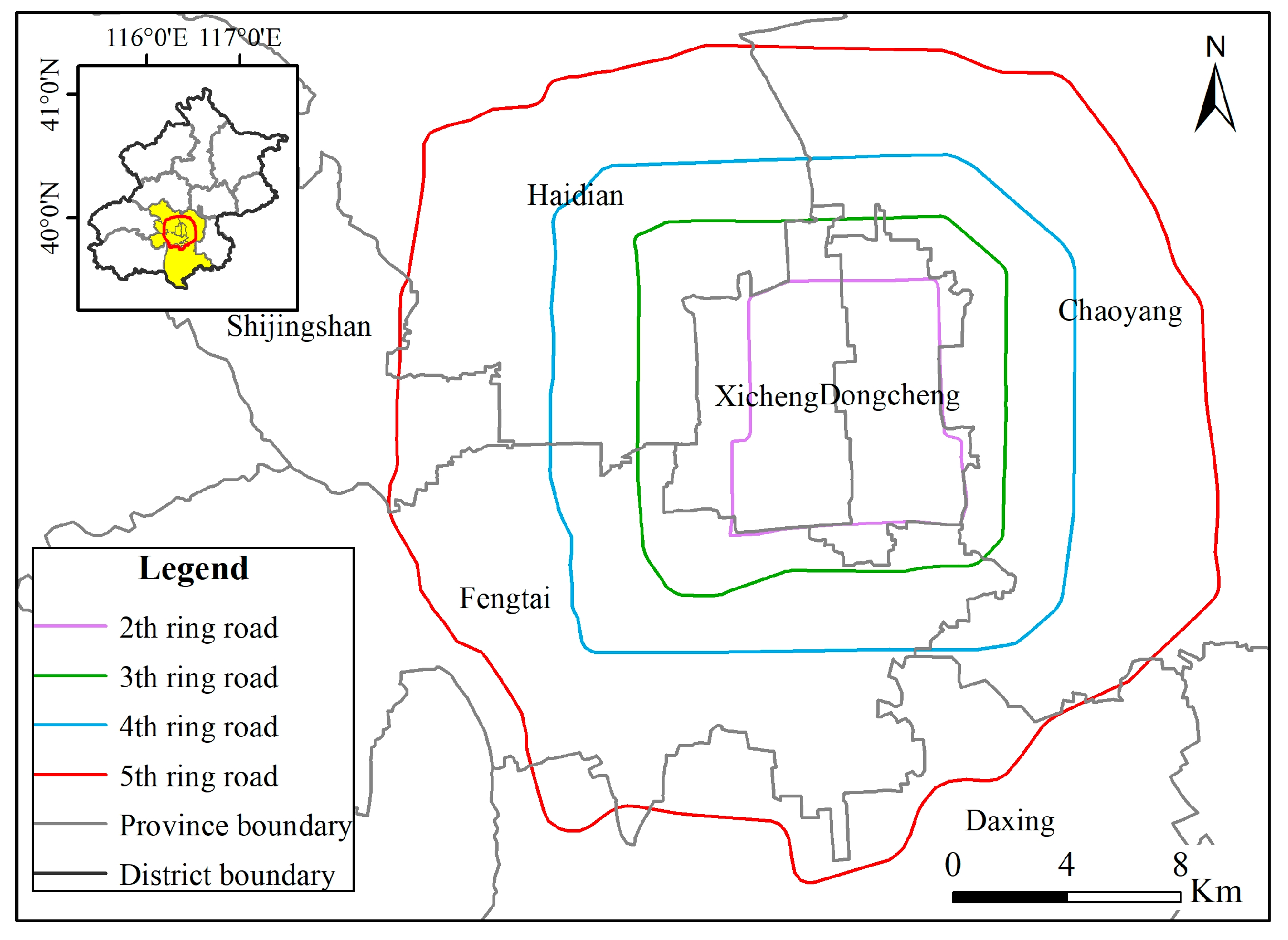
2.1. Study Area

Beijing is the capital of the People’s Republic of China and is located in the north of the North China Plain, with a total area of 16,410.54 km2. As the second most populous city in China, Beijing has experienced rapid urban expansion since the adoption of a social market economy in 1984 [18,19]. By the end of 2019, the city had 16 districts under its jurisdiction, with a permanent resident population of 21.536 million, of which 18.5 million were urban residents, representing an urbanization rate of 86.6%. Urban expansion and rapid land-use change have led to the rapid decrease in UGS and an increasingly serious contradiction between urbanization and public ecological interests [20]. In order to reduce the negative impacts of UGS loss, the People’s Government of Beijing has implemented a number of UGS planning policies. However, due to the practical difficulties of urban development, some UGS planning has not achieved the optimal desired results [20]. Therefore, it is necessary to conduct further research on its UGS and put forward corresponding optimization suggestions. The area within the 5th Ring Road of Beijing mainly includes a total of seven districts, namely the Dongcheng, Xicheng, Chaoyang, Haidian, Shijingshan, Fengtai and Daxing districts (Figure 1). Due to the dense population, developed economy and intensive land development, the area within the 5th Ring Road is a typical area with the most prominent contradiction between humans and land in Beijing. Therefore, in this study, Beijing’s 5th Ring Road was selected as the research area; the current situation of the ES supply of the UGS ecosystem and the spatial distribution of human demand for ESs was evaluated, and the spatial pattern of UGS was optimized based on the balance of supply and demand.

2.2. Data Sources and Processing

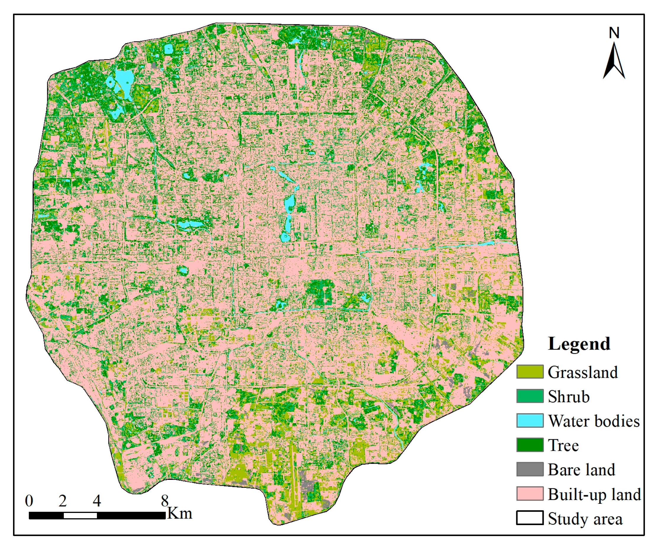
2.2.1. GF-2 Imagery and Land Use Classification

Six GaoFen-2 (GF-2) images acquired on 16 August, 2019 were obtained for land use classification and UGS information extraction in the region of the 5th Ring Road of Beijing. The GF-2 data were obtained from the China Center for Resources Satellite Data and Application (http://www.cresda.com/CN/index.shtml, accessed date: February 2020). Launched on 19 August, 2014, the GF-2 satellite is a Chinese civilian high-resolution optical satellite and is equipped with both a panchromatic sensor and a multispectral sensor. The GF-2 data downloaded are a level 1A relative radiometric correction product, and a series of pre-processing operations (such as radiometric correction, atmospheric correction, image fusion and geometric fine correction) are required for the original image, so as to eliminate the geometric distortion caused by radiation error and topographic relief caused by the influence of the sensor itself and the atmosphere.
In view of the characteristics of GF-2 data (e.g., high spatial resolution, large data volume, rich spatial information and obvious texture features, etc.), the spectral features, texture feature geometry and other information of the image were fully utilized, and multiscale segmentation and spectral difference segmentation were integrated to obtain the optimal segmentation results. The land use classification results of the study area were obtained via the e-Cognition software platform and the multi-feature object-oriented approach [21,22]. According to our research objectives and the field survey, the land use and land cover system in this study area consisted of six classes: tree, shrub, grassland, built-up land, water bodies and bare land. The classification results are shown in Figure 2, and the area proportion of each land use type is as follows: tree, 14.16%; shrub, 14.42%; grassland, 10.51%; built-up land, 58.91%; water bodies, 1.33%; bare land, 0.67%.

2.2.2. Basic Data of Population Spatialization

In addition to land use and land cover, the spatialization of a population also requires data such as points of interest (POIs), nighttime light, water and road networks.
POIs mainly refer to some geographical entities that are closely related to human life and abstract as points. With the advantages of rich data volume, strong practicality, high positioning accuracy and the ability to effectively reflect the features of human space activity range and regional development level, POI data have been widely used in population data spatial mapping [23,24] and urban functional area identification [25,26]. Thus, POI data are the basis of the spatialization of the population. In this study, POI data were acquired in 2018 via the application programming interface (API) provided by Amap of China (https://www.amap.com/, accessed date: February 2020). In the area within the 5th Ring Road of Beijing, a total of 672,136 POI records were obtained.
Water and road network data were collected from OpenStreetMap of British(OSM) (https://www.openstreetmap.org, accessed date: February 2020). After revision and improvement in recent years, the accuracy of OSM data in urban areas has been widely recognized [27]. The classification of the Beijing road network data downloaded from OSM is relatively large, and there is little redundancy. In this study, with the assistance of Amap, redundant roads and unnecessary details were deleted and mainly the trunk, primary, motorway, secondary, tertiary, residential and service roads were preserved.
As remote sensing image data that can represent the characteristics of population activities, nighttime light data have been widely used in population spatialization research [28,29]. Luojia 1-01 (LJ1-01) is equipped with a highly sensitive camera that can identify weak light sources and has a finer spatial resolution than traditional nighttime light data. Therefore, the LJ1-01 nighttime light data from 23 November 2018 (http://59.175.109.173:8888/, accessed date: April 2020) were used as the basic data for population spatialization in this study. The standard storage format of the original data downloaded from the website is INT32. The user should convert the INT32 standard images to the radiance according to the radiance conversion formula:
L = D N 3 / 2 · 10 10
where L is the input radiance ( W / ( m 2 · s r · μ m ) ), and DN is the digital number of LJ1-01 images.

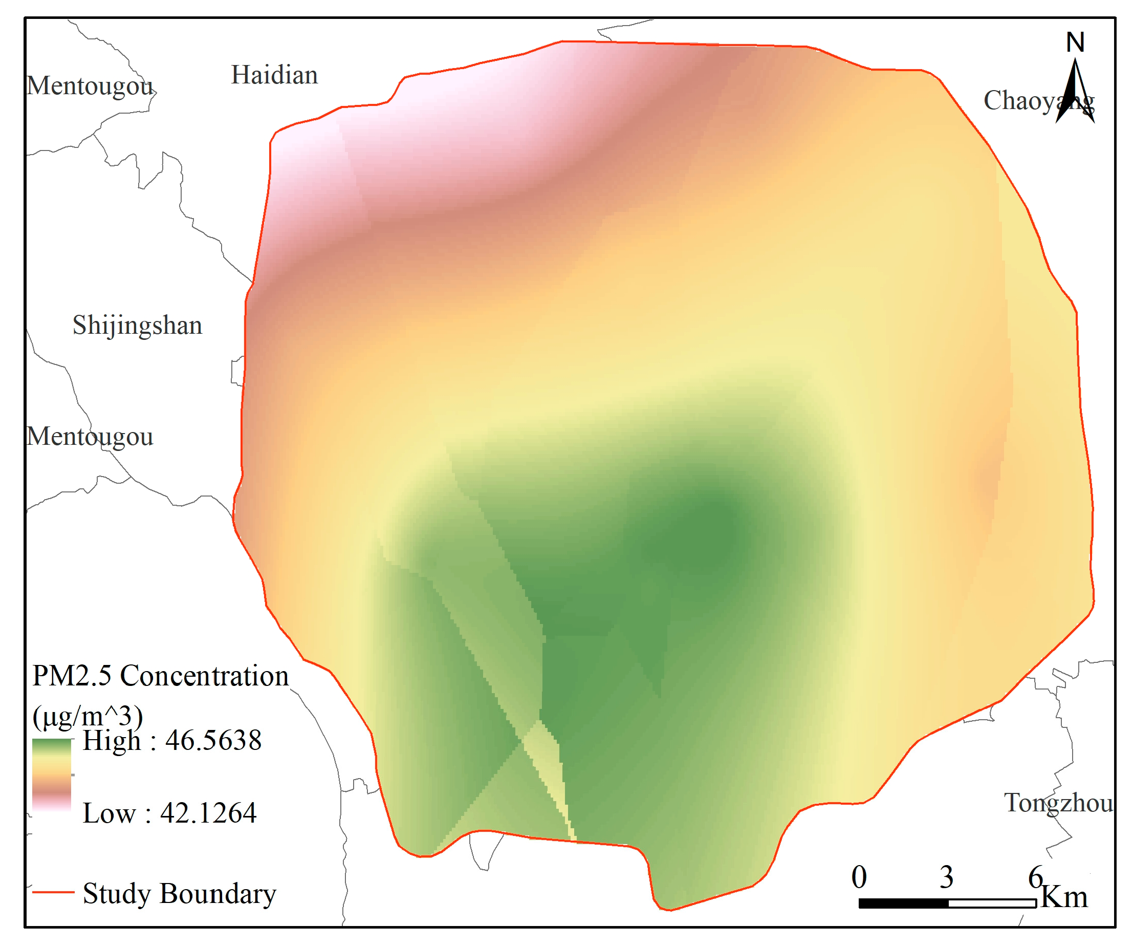
2.2.3. PM2.5 Distribution

PM2.5 data were obtained from hourly station monitoring data. There are 35 ambient air quality monitoring stations in Beijing, including 14 within the 5th Ring Road. Due to air circulation, gas diffusion and other influences, the regional environment has a great impact on the PM2.5 concentrations in the adjacent areas. Therefore, this study used the Kriging spatial interpolation method to estimate the annual mean PM2.5 concentration ( μ g / m 3 ) in the unknown region based on the annual mean PM2.5 concentration of 14 stations within the 5th Ring Road and six surrounding stations. First, the hourly monitoring data of 20 stations were sorted out to remove missing and invalid data and calculate the annual average PM2.5 concentrations at each monitoring point. Second, the PM2.5 spatial interpolation map was cut out by the boundary of the study area, and a spatial distribution map of PM2.5 within the 5th Ring Road of Beijing was finally obtained (Figure 3).

2.2.4. Leaf Area Index (LAI) Data

Leaf area index (LAI) refers to the sum of the leaf areas of vegetation per land area unit, which can reflect the canopy structure of vegetation. The existing LAI data product (Moderate-resolution Imaging Spectroradiometer, MODIS) has a low spatial resolution, which is more suitable for studies at the regional scale, and has poor applicability for studies within urban areas. In this study, UGS within the 5th Ring Road of Beijing was mainly divided into three types: tree, shrub and grassland. Based on the ENVI5.3 software, the green space normalized difference vegetation index (NDVI) was calculated. Combined with the LAI-NDVI algorithm (Table 1) and GF-2 remote sensing images, the LAI of green space within the 5th Ring Road of Beijing was estimated.

3. Methods

The Common International Classification of Ecosystem Services (CICES) was intended as a reference classification and has been widely used in ES research [32]. In the latest version (V5.1), services are grouped into three sections: (1) provisioning, (2) regulation and maintenance and (3) cultural. Different types of ESs meet different human needs in terms of basic raw materials, physical health and healthy social relationships and are closely related to human well-being.
Polluted air affects the human respiratory system, leading to an increase in the incidence of various respiratory diseases [33]. Plants can trap, intercept and adsorb atmospheric soot and dust particles; are low-cost and have ecological benefits [34,35]. A dense population and buildings lead to the formation of relatively closed spaces in cities, resulting in reduced gas exchange and increases in radiation heat and other problems [36,37]. The functions of carbon sequestration and oxygen release in UGSs are particularly important to improve urban air quality and alleviate the problem of hypoxia in urban environments [38,39]. Therefore, in this study, PM2.5 purification and carbon sequestration ESs, which are in high demand by urban residents, were selected as quantitative factors. We evaluated the service of the UGS ecosystem and applied it as the evaluation basis of the ES supply of UGS.
ES spatial mapping is a process of spatializing the quantitative results of ESs according to research or decision-making needs and the appropriate mapping methods. In this study, the distribution of UGS ES supply and demand was studied at multiple scales, the conceptual framework of methodology is shown in Figure 4. First, the UGS ES supply and demand and the budgets of them were analyzed on the administrative unit scale, and the administrative units in which the supply was unable to meet the demand were extracted as the areas to be optimized. Then, the analysis was carried out on a finer scale for the area to be optimized, whereby the analysis of UGS ES supply and demand and the budgets of them was carried out on a 1-m grid scale.

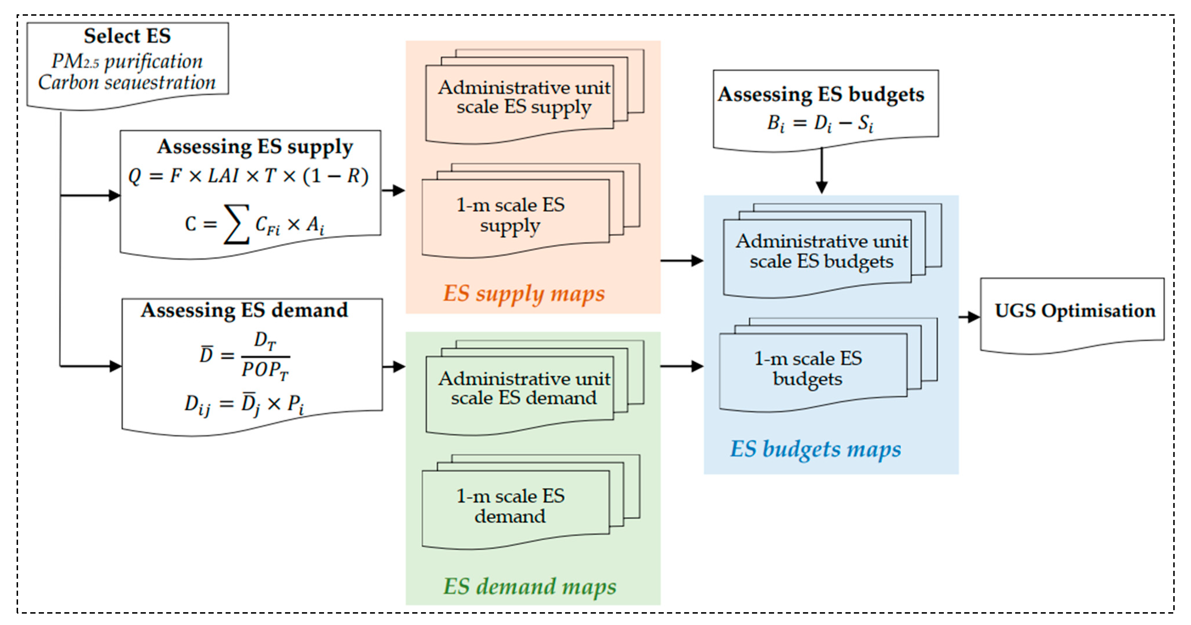
3.1. Mapping ES Supply

3.1.1. Assessment of UGS ES Supply

We did not consider wet settlement under the influence of rain and snow scour, but rather only considered the physical settlement process of PM2.5 and used the dry deposition model to calculate the purification effect of UGS on PM2.5. The principle of dry deposition has been applied in many studies of urban forest absorption of atmospheric pollutants [40,41]. The calculation formula for daily reduction in PM2.5 in the UGS based on the dry deposition model is as follows:
Q = F × L A I × T × ( 1 R )
F = V × C
where Q represents the daily reduction in PM2.5 (g/m2); F represents the dry deposition flux of PM2.5 per unit blade area; L A I represents the leaf area index; T represents the effective reduction time (s) of UGS for PM2.5, which is based on the daily scale; R is the coefficient of resuspension; V represents the dry deposition rate and C represents the PM2.5 concentration. Previous studies have shown that the settlement rate and weight suspension coefficient of PM2.5 on the surface of green leaves are related to wind speed [42]. The mean wind speed in the vegetation growing season in Beijing in 2019 was 1.98 m/s; therefore, the V and R values are 0.09 cm/s and 3%, respectively.
Carbon sequestration by plants was defined as the total abovementioned carbon storage in this study, and the carbon sequestration capacity of different plant types in UGS was quantified based on existing research indicators [43].
C = C F i × A i
where C represents the total carbon sequestration of the UGS ecosystem (kg/yr.), C F i represents the carbon sequestration amount per unit area of different UGS (kg/yr.m2; tree, 10.64 kg/m2∙yr.; shrub, 6.7 kg/m2∙yr.; grassland, 0.17 kg/m2∙yr.) and A i represents the total area of different UGS types.

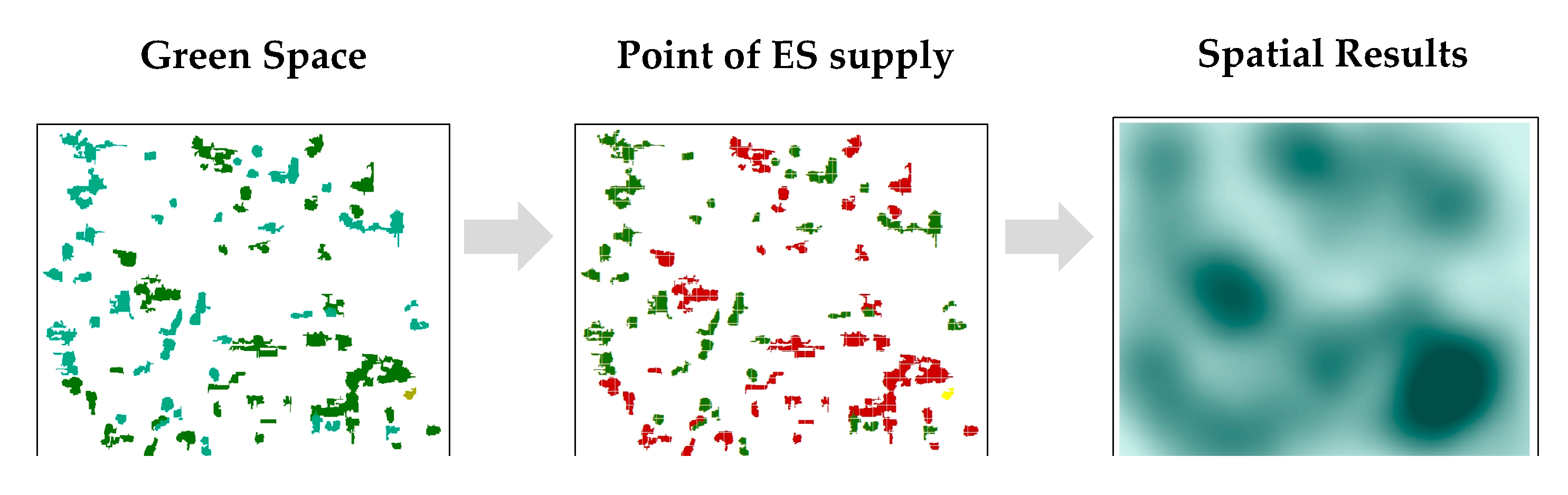
3.1.2. Mapping ES Supply at Two Scales

Spatialization of ESs at the administrative unit scale mainly uses the vector data of administrative units to conduct regional statistics on the evaluation results of ESs of green patches to obtain the sum of ESs provided by all green spaces in each administrative unit. The UGS ES supply at the 1-m scale was spatialized mainly by using the kernel density analysis method. The kernel density analysis model in GIS spatial analysis can disperse the value of known phenomena or elements over the entire surface, thus generating a continuous surface from discrete point or line data. Taking the kernel density analysis of points as an example, the principle is to assume that the top of each known point element is covered with a smooth surface. The surface value is the highest at the position where the point is located, gradually decreases as the distance from the point increases and is zero at the position where the distance from the point is equal to the search radius. The volume between this smooth surface and the plane below it is equal to the property of that point. After conducting experiments every 100 m in the range of 0–1 km, we finally determined the kernel density radius of 500 m, which can ensure that ESs can be distributed recursively with distance in space. Each grid value of the output data is equal to the sum of the values of all of the core surfaces on the grid. The green patch of the administrative unit to be optimized is converted into point data, and the attribute of the point is the quantitative value of the green patch ES supply. The kernel density analysis tool of Arcgis10.6 was used to spatialize the supply of the administrative unit to be optimized on a grid scale (Figure 5).

3.2. Mapping Human Demand of UGS ES

3.2.1. Indicator of UGS ES Demand

The UGS ES demand was calculated in the same unit as the supply in order to guarantee the direct comparability of supply and demand. According to the definition of ES demand that we adopted in this study, it is the sum of all ecosystem goods and services currently consumed or used in a given region in a given period of time. The study area was regarded as an ecosystem as a whole, and the sum of ESs consumed or used by people in a certain period was calculated as the ES demand. UGS is an important part of urban green infrastructure and public service facilities, and every urban resident has an equal right to enjoy the ESs equally. Based on this, the per capita demand of ESs was calculated based on demographic data. Then, the spatial distribution of the population was used to map the UGS ES demand.
D ¯ = D T P O P T
D i j = D ¯ j × P i
where D ¯ is the per capita ES demand; D T is the total demand for ESs within a given time and region; P O P T is the total population of the study area; D i j is the population demand for the j ES in the i region; D ¯ j is the per capita demand of j ES and P i is the population of i region or grid.

3.2.2. Mapping ES Demand at Two Scales

The UGS ES demand at the administrative unit scale was obtained by multiplying the demographic data of each administrative unit by the per capita demand index of UGS ES, while the UGS ES demand at a 1-m grid scale was obtained by multiplying the 1-m grid scale population data by the per capita demand index. Therefore, spatialized population data are the main data for analyzing the UGS ES demand at the 1-m grid scale.
Traditional population data usually refer to the demographic data, which cannot reflect the spatial distribution characteristics of the population. In this study, we adopted a multi-source data fusion model to conduct grid processing of population data in the study area. Based on the road network density, distance from water bodies, slope, nighttime light, land use type and 10 types of POI that are most relevant to demographics, a spatialized evaluation index system of the population was built. Different land use types have different effects on the spatial distribution of the population, which need to be quantified. According to the expert scoring method, weights were assigned to different land use types: water = 0 points; unused land = 1 point; forest land, shrub and grassland = 2 points; and built-up land = 9 points. ArcGIS10.6 was used to calculate the core density of the road network along with POI data as well as the distance from the water bodies. Buffer radii of 40, 20 and 10 m were established for roads of different levels [44], and a kernel density analysis was carried out on road network data in the study area, with the buffer radius as the weight. Finally, the value range of each indicator was normalized to 0-10 so that it was consistent with the value range of the land use type and was convenient for subsequent weighted processing.
Determination of the index weight is a core part of constructing an index system in multi-attribute evaluation. We used principal component analysis to determine the influence weight of each index on the population spatial distribution:
ω i = δ i i = 1 p δ i
δ i = j = 1 m l j i × j
where ω i represents the weight of each index; δ i represents the factor comprehensive score of each index; j represents the variance contribution rate of each principal component and l j i represents the score coefficient of each index in different principal components.
After the weight of each index was obtained, Equation (9) was used to calculate the comprehensive weight of the population distribution in the study area:
W = i = 1 m ω i × P i j
where W represents the combined weight of each grid and P i j represents the normalized value of index X i in different grids. The population of each grid can be determined by Equation (10):
P O P k = P O P × W k W k
where P O P k is the population of the k grid; P O P is the demographic data of the sub-district where the grid is located and W k is the sum of the comprehensive weight values of all grids of the sub-district where the grid is located.

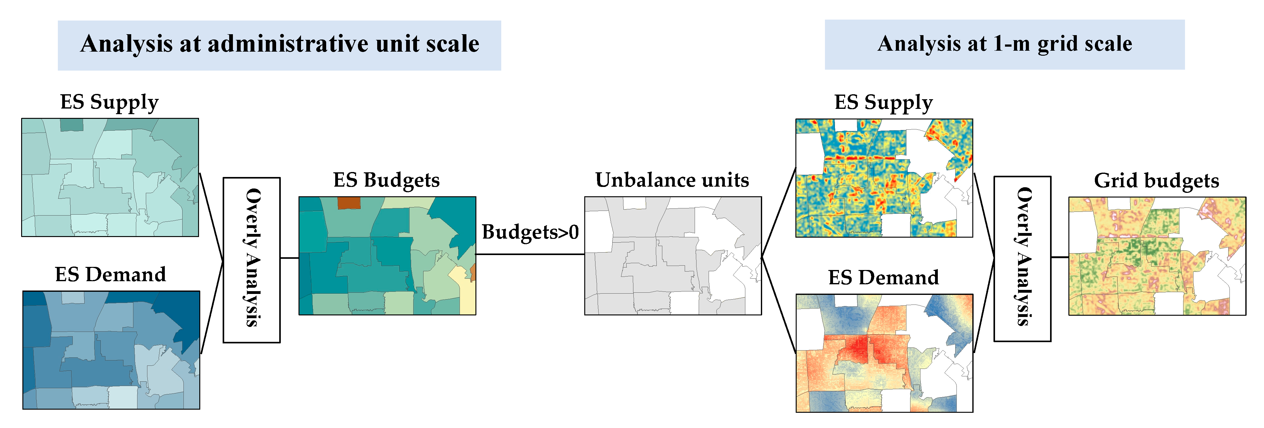
3.3. Mapping Budgets of ES Supply and Demand

Assessing the matches and mismatches between ES supply and demand usually requires assessing demand in the same units as those used for supply to obtain a budget ratio indicating that ES is in undersupply, neutral balance or oversupply [16,45,46]. According to the criteria described above, the supply and demand of the same ESs were quantified in the same unit in this study. The budget of UGS ES supply and demand was calculated using Equation (11):
B i = D i S i
where D i represents the UGS ES demand; S i represents the UGS ES supply; B i represent the budgets of UGS ES supply and demand; and B i > 0 indicates that the UGS ecosystem service supply cannot meet human demand, while B i 0 indicates that the UGS ecosystem service supply can meet human demand.
First, based on the evaluation results of the UGS ES supply and demand at the administrative unit scale, the balance of UGS ES supply and demand at the administrative unit scale was analyzed using an overlay analysis. This was carried out in order to express sensitive areas with a weak spatial distribution of UGS ESs in a quantitative, intuitive and visual form and to identify the administrative units where the ES supply could not satisfy the demand ( B i > 0). Then, the administrative units with an imbalance of supply and demand of ESs were extracted to further refine the spatial distribution of their UGS ESs. Similarly, the balance of the UGS ES supply and demand on the 1-m grid scale was determined (Figure 6).

3.4. UGS Optimization

The results of the analysis of UGS ES supply and demand on two scales are the basic data of landscape optimization. This means that the evaluation results of ES supply and demand at the scale of administrative units are used to determine the UGS optimization strategy and optimal total amount of sub-districts with an unbalanced supply and demand, while the evaluation results of ES supply and demand at the 1-m grid scale are used to determine the optimization area of the administrative units to be optimized. There are various reasons for the imbalance between UGS ES supply and demand. In this study, administrative units for which the ES supply was unable to meet the demand were classified and discussed, and different optimization strategies are proposed (Table 2).
The greater the budget between ES demand and supply is, the more unbalanced the supply and demand is. According to the evaluation results of the 1-m grid scale ES supply and demand, the regions with unbalanced supply and demand were equally divided into (1) severe ES shortage areas (66% B m a x B m a x , where B m a x represents the maximum budget of UGS ES supply and demand at the 1-m grid scale of the administrative unit to be optimized, as discussed below), (2) moderate ES shortage areas (33% B m a x –66% B m a x ); and (3) mild ES shortage areas (0–33% B m a x ) according to the budgets of supply and demand from large to small. Moreover, the severe shortage area with the greatest difference between ES supply and demand was taken as the UGS optimization area.

4. Results

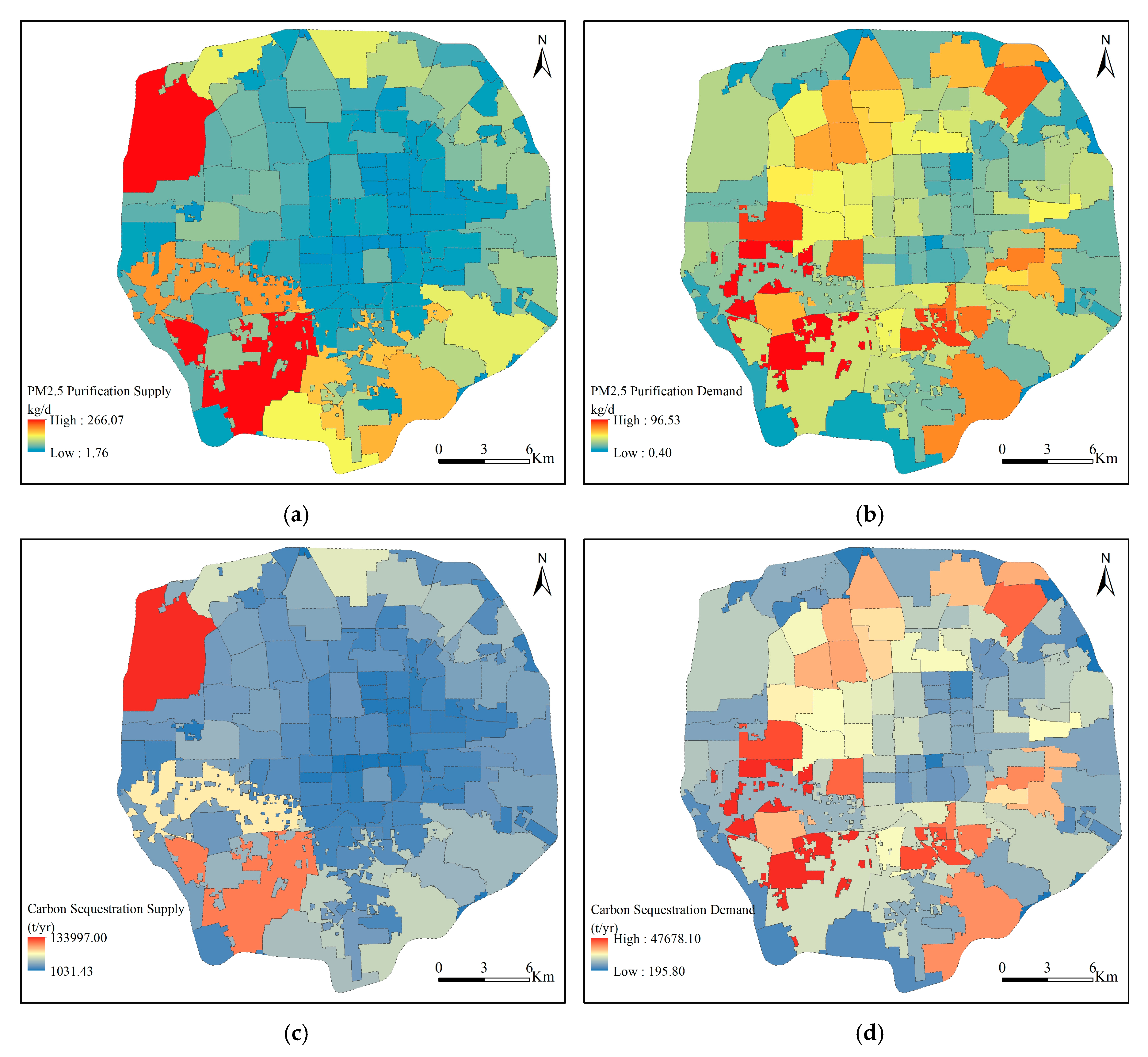
4.1. Evaluation Results of the UGS ES in Study Area

According to the analysis results, the supply of PM2.5 purification and carbon sequestration services for the total UGSs and different UGS types within the 5th Ring Road of Beijing is shown in Table 3. It can be seen that the amount of ESs provided by different UGS varies greatly due to the difference in area and ES supply capacity of them. Trees are the main provider of ESs. The supply of PM2.5 purification from trees is 45.31% of the total supply, and the supply of carbon sequestration from trees reaches 60.50% of the total supply. The ES supply from trees per unit area is also larger than that from shrubs and grassland, especially for carbon sequestration. The annual carbon sequestration per unit area of trees is 1.59 times that of shrubs and 62.59 times that of grassland.

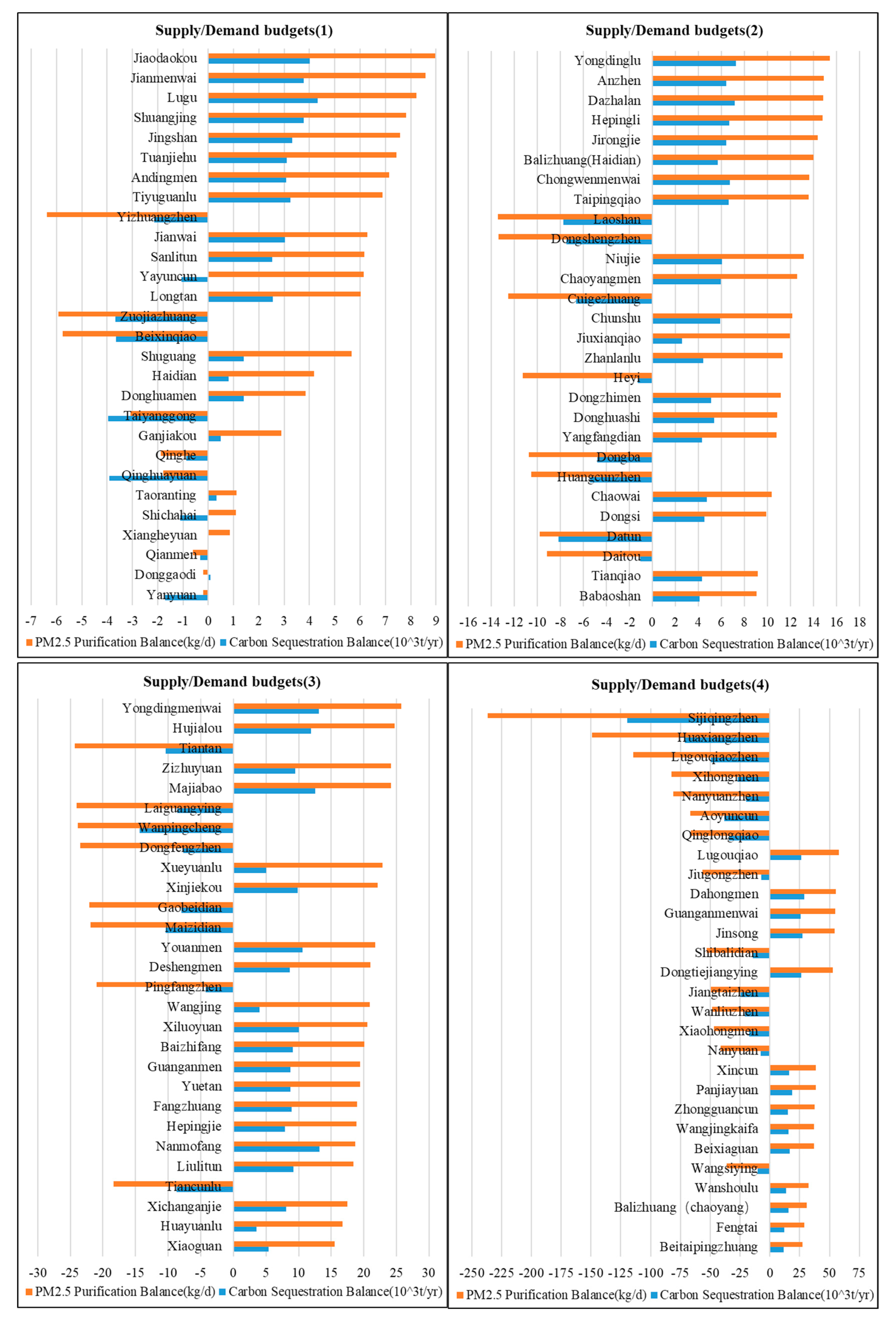
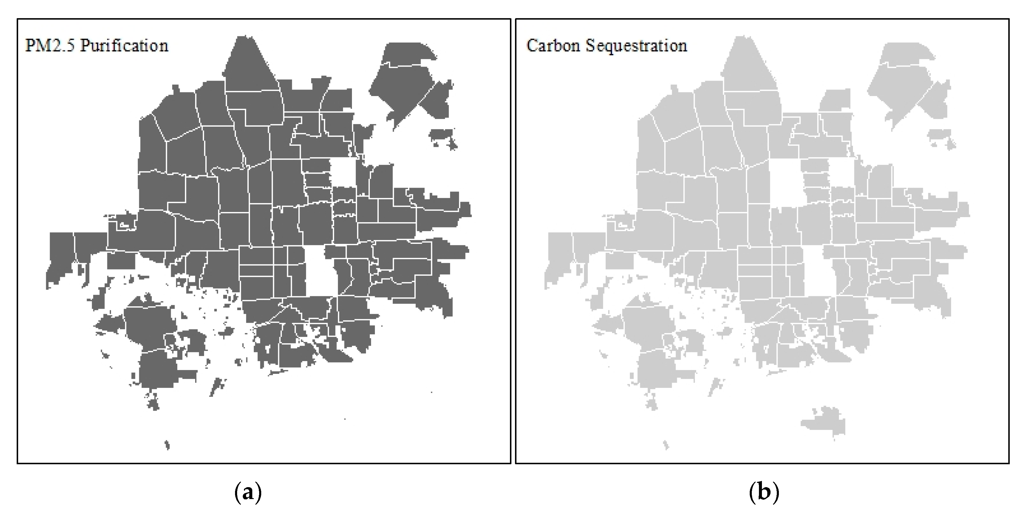
4.2. ES Supply and Demand at Administrative Units Scale

The resulting maps of the area within the 5th Ring Road of Beijing show the spatial distribution of the UGS ES supply and demand in different administrative units (Figure 7). The quantification results of the ES supply show that the total amount of PM2.5 purification of the UGS in the study area was 3441.58 kg/d. The Sijiqing sub-district had the largest PM2.5 purification supply of 266.07 kg/d, accounting for 7.73% of the total supply. The PM2.5 purification supply of the Dazhalan sub-district was the smallest at 1.76 kg/d, accounting for 0.05% of the total supply. The Shuangjing and Dongtiejiangying sub-districts displayed comparatively intermediate values, with total supplies of almost 18.83 and 18.93 kg/d, respectively. The supply of carbon sequestration ESs also showed the highest values in the Sijiqing sub-district, which is 133,997.20 t/yr., accounting for 7.88% of the total supply in the study area (1,699,900.83 t/yr.). The carbon sequestration supply of the Dazhalan sub-district was the smallest, which is 1031.43 t/yr., accounting for 0.06% of the total supply. The supply in the Zuojiazhuang and Hepingjie sub-districts displayed comparatively intermediate values, with a total supply of nearly 9781.33 and 10,170.21 t/yr., respectively, accounting for 0.58% and 0.60% of the total supply, respectively.
As the ES demand depends on population density, ES mapping is consistent with the spatial distribution of the population. The quantification results of ES demand showed the highest values in the Lugouqiao sub-district (PM2.5 purification demand: 96.53 kg/d; carbon sequestration demand: 47,678.12 t/yr.), which has the largest population, while the lowest values were recorded in the Cuigezhuang sub-district (PM2.5 purification demand: 0.40 kg/d; carbon sequestration demand: 195.81 t/yr.), which has the smallest population.
Following the criteria described above, matches and mismatches between ES supply and demand were identified, and the results are shown in Figure 8. The results show 74 sub-districts where the ES demand was not met by the ES supply (Figure 9). Among them, in the Yayuncun, Shichahai and Xiangheyuan sub-districts, the PM2.5 purification demand was not totally met by the supply, while in the Donggaodi sub-district, the carbon sequestration demand was not completely met by the supply, and the supply of two kinds of ESs in the other 70 sub-districts did not meet the demand.

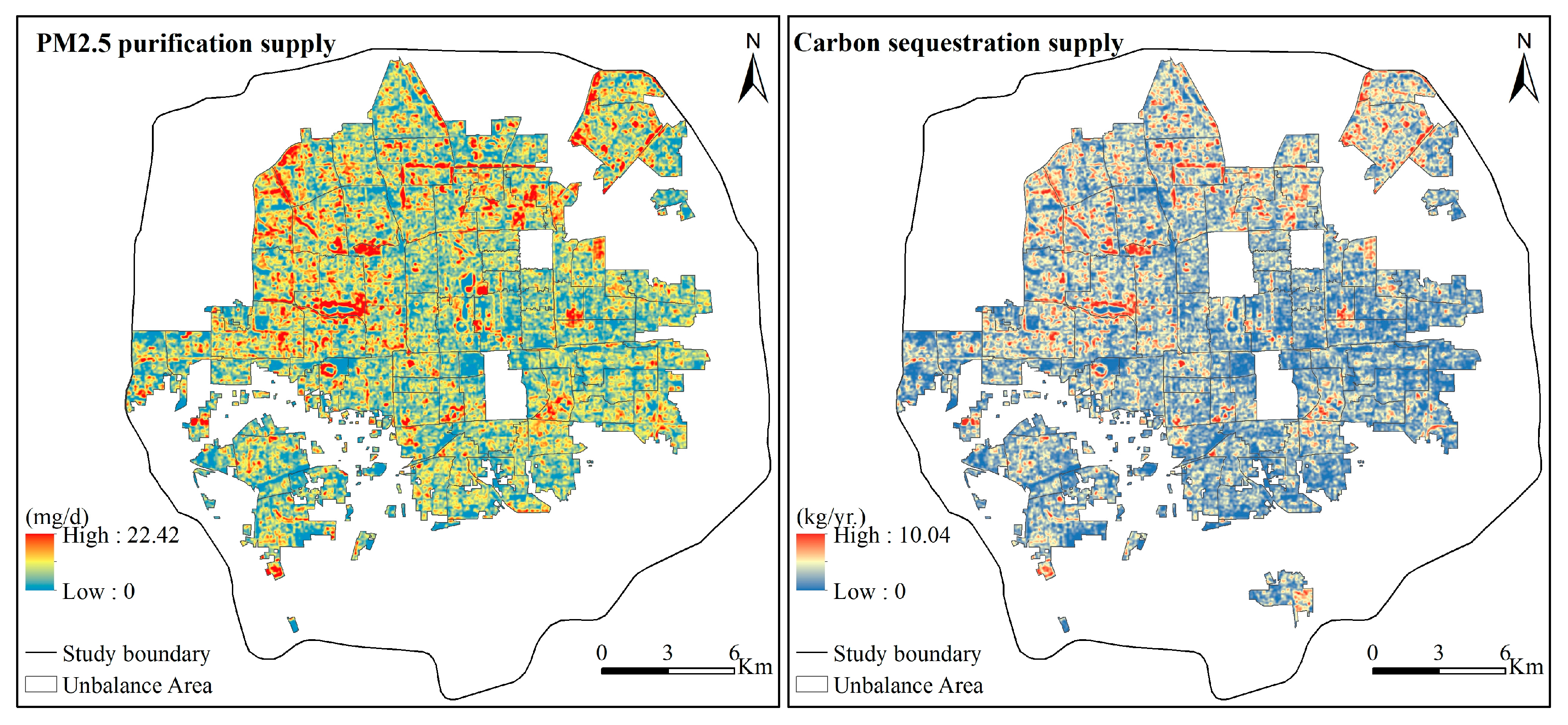
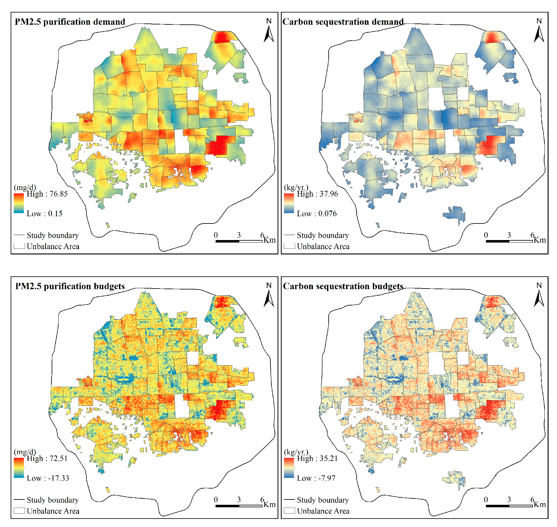
4.3. ES Supply and Demand at 1-m Grid Scale

The above methods were used to calculate the grid supply and demand of PM2.5 purification and carbon sequestration services for sub-districts with an unbalanced ES supply and demand. As shown in Figure 10, the maximum daily supply of PM2.5 purification services per unit area was 22.42 mg/d, while the maximum daily demand for PM2.5 purification service per unit area was 75.85 mg/d, i.e., 3.38 times the maximum supply. The maximum annual supply of carbon sequestration services per unit area was 10.04 kg/yr., while the maximum annual demand for carbon sequestration service per unit area was 36.96 kg/yr., i.e., 3.55 times the maximum supply. There was considerable spatial heterogeneity in the distribution of supply and demand of the two services. Among them, the maximum budget value between the unit area demand and supply of PM2.5 purification services was 72.51 mg/d, and the maximum budget value between the unit area demand and supply of carbon sequestration services was 35.21 kg/yr.

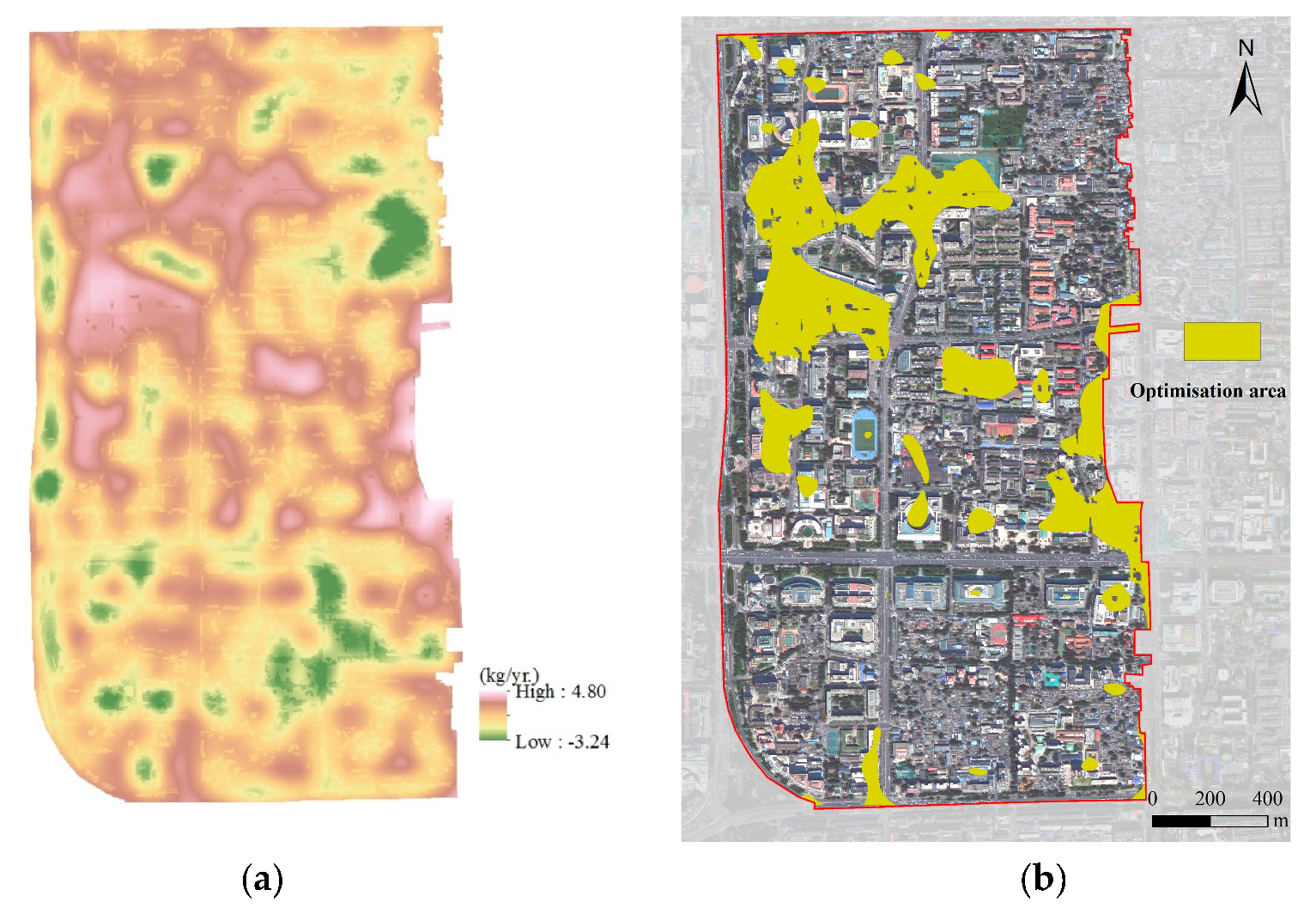
4.4. Landscape Pattern Optimization of UGS

According to the analysis results of ESs at different scales described above, there were obvious spatial differences in the distribution of supply and demand of PM2.5 purification and carbon sequestration services. The same ES service showed supply and demand differences in different administrative units, and the distribution of supply and demand of different services in the same unit also differed. Therefore, different strategies should be proposed for different protection purposes.
Based on the evaluation results of the carbon sequestration service supply and demand of UGSs within the 5th Ring Road of Beijing, the sub-districts in which the supply was lower than the demand were classified according to the above methods (Table 4). According to the results, among the 71 sub-districts where the supply of carbon sequestration service was lower than the demand, the imbalance of supply and demand in 11 sub-districts belonged to the “Lack of green space” type; 8 sub-districts belonged to the “Unreasonable structure of green space” and 52 other sub-districts belonged to the “Comprehensive” type. Therefore, the green rate of most sub-districts failed to reach the level of the overall green rate of the 5th Ring Road, and these sub-districts existed as an unreasonable phenomenon of green space structure.
The optimal locations of UGS for different sub-districts need to be determined according to the evaluation results on the grid scale. This study took the Jinrongjie sub-district as an example to illustrate the UGS optimization identification method. The evaluation results of the Jinrongjie sub-district on the grid scale show that the maximum budget between the carbon sequestration service demand and supply per unit area was 4.80 kg/yr. Therefore, according to the budget between demand and supply, the regions with an unbalanced supply and demand of carbon sequestration services in the Jinrongjie sub-district were divided as follows: areas with a budget between 0 and 1.60 kg/yr. belonged to the mild ES shortage area category; areas with a budget between 1.60 and 3.20 kg/yr. were moderate ES shortage areas; areas with a budget between supply and demand of between 3.20 and 4.80 kg/yr. were severe ES shortage areas. Moreover, the severe ES shortage areas of ES supply were taken as the UGS optimization area, this is shown in Figure 11.

5. Discussion

5.1. Innovations of UGS Landscape Pattern Optimization Based on ES Evaluation

We built a theoretical method and technical framework of UGS optimization based on ES supply and demand. Taking the UGS optimization within the 5th Ring Road of Beijing as an example, the feasibility and reliability of the proposed method were demonstrated. The differences between our study and the existing studies are as follows.
First, this study analyzed the ES supply and demand at multiple scales and at an even finer scale than existing studies did. The ES supply and demand have different matching patterns at different spatial scales; thus, the relationship between ES supply and demand at different scales should be comprehensively analyzed [47]. Most of the existing studies on the spatial analysis of ES supply and demand are based on administrative units [48], ecosystems [49] or land use types [16], and they were conducted on a single scale. However, such large-scale studies are insufficient to fully reflect the internal heterogeneity of ES supply and demand. Therefore, our work is meaningful to further the study on a finer scale.
Second, the research results of ES are applied to the UGS optimization, which makes up for the lack of consideration of population distribution and ES demand in the process of UGS construction. With increasing attention being paid to the relationship between ESs and human well-being, some researchers have evaluated the spatial matching of UGS ES supply and demand, which is helpful in urban planning [50,51]. However, most of these studies do not provide practical guidance for urban green space planning [52]. In this study, based on the results of the UGS ES supply and demand assessment at two scales, we provide specific theoretical optimization suggestions for administrative units with unbalanced ES supply and demand, including UGS optimization schemes and locations (see Section 3.4). Therefore, our work is meaningful in assisting UGS planning, which will improve the efficiency of government planning departments.
Third, the UGS ES supply and demand were quantified using the same units in order to be comparable. Due to the different research objects, it is difficult to construct a relationship between UGS supply and demand [51]. This study provides a simple and easy-to-use method to evaluate and map multiscale supply and demand relationships for UGSs and provides a technical framework for conducting research on UGS ES supply and demand at an urban or regional scale.

5.2. Limitations and Future Directions

Some uncertainties and limitations of our work need to be considered. Firstly, due to the limitation of data acquisition and research time, this study only used PM2.5 purification and carbon sequestration as the means of UGS optimization and, finally, used an administrative unit within the 5th Ring Road of Beijing to verify the UGS optimization method. The next step is to continue to evaluate some other ESs so that more ESs can be comprehensively evaluated to guide UGS planning. Secondly, the UGS ES demand is related to the population [53], social and economic characteristics [54] and other factors. However, the demand model in this study only considers the population density as an indicator. In the future, more factors should be considered to conduct a more comprehensive and in-depth simulation assessment.

6. Conclusions

To evaluate the distribution of UGS ES supply and demand in different areas of a city, and to achieve on-demand planning, which requires remote sensing and other spatial information technologies to obtain the status quo of the UGS, it is necessary to make an accurate quantitative assessment of the spatial distribution of the UGS ES supply and demand by using ecological knowledge and GIS. Only on the basis of scientific, accurate and objective quantification of the UGS ES spatial supply and demand can a UGS pattern be effectively adjusted and optimized.
This study presents a multiscale analysis method for the spatial distribution of UGS ES supply and demand and makes different UGS optimization suggestions based on the evaluation results. We also analyzed the balance between the supply of ESs and the demand for UGS within the 5th Ring Road of Beijing, identified and classified the sub-districts where the carbon sequestration service supply cannot meet the demand and presented different UGS optimization suggestions. Compared to existing research, our work has three unique points: (1) We developed a multiscale analysis method for balancing UGS ES supply and demand and directly compared the supply and demand in spatially explicit maps; (2) we classified the administrative units with unbalanced ES supply and demand and put forward different UGS optimization suggestions; (3) we applied the multiscale evaluation results of ES supply and demand to UGS planning to provide the spatial location and relevant demand information of the UGS ES-weak area for the urban planning departments. In future work, we will investigate the optimized green space at a more detailed scale and further evaluate the other UGS ecosystem services.

Author Contributions

Conceptualization, Qinqin Liu and Kai Yin; methodology, Qinqin Liu, Yichen Tian and Kai Yin; software, Qinqin Liu; validation, Qinqin Liu, Yichen Tian and Kai Yin; formal analysis, Qinqin Liu; investigation, Qinqin Liu; resources, Kai Yin and Huiping Huang; data curation, Kai Yin and Huiping Huang; writing—original draft preparation, Qinqin Liu; writing—review and editing, Kai Yin, Yichen Tian, Feifei Zhang and Fangmiao Chen; visualization, Qinqin Liu; supervision, Kai Yin and Huiping Huang; project administration, Yichen Tian, Kai Yin and Huiping Huang; funding acquisition, Kai Yin and Huiping Huang. All authors have read and agreed to the published version of the manuscript.

Funding

This study was funded by the Major Project of High Resolution Earth Observation System (06-Y30F04-9001-2022) and the National Natural Science Foundation of China (41471423)

Data Availability Statement

The data presented in this study are available on request from the corresponding author. The data are not publicly available due to privacy.

Conflicts of Interest

The authors declare no conflict of interest.

References

  1. Niemelä, J. Ecology and urban planning. Biodivers. Conserv. 1999, 8, 119–131. [Google Scholar] [CrossRef]
  2. Michelle, K.; Jaime, F.; Thomas, M.; Charles, B. Urban Green Space and Its Impact on Human Health. Int. J. Environ. Res. Public Health 2018, 15, 445. [Google Scholar]
  3. Aronson, M.F.; Lepczyk, C.A.; Evans, K.L.; Goddard, M.A.; Lerman, S.B.; MacIvor, J.S.; Nilon, C.H.; Vargo, T. Biodiversity in the city: Key challenges for urban green space management. Front. Ecol. Environ. 2017, 15, 189–196. [Google Scholar] [CrossRef] [Green Version]
  4. Bowler, D.E.; Buyung-Ali, L.; Knight, T.M.; Pullin, A.S. Urban greening to cool towns and cities: A systematic review of the empirical evidence. Landsc. Urban Plan. 2010, 97, 1–155. [Google Scholar] [CrossRef]
  5. He, C.; Liu, Z.; Tian, J.; Ma, Q. Urban expansion dynamics and natural habitat loss in China: A multiscale landscape perspective. Glob. Chang. Biol. 2014, 20, 2886–2902. [Google Scholar] [CrossRef] [PubMed]
  6. Jin, X.; Dong, S.; Zhou, C.; Li, Y.; Li, Z. Ecological environmental problems in Chinese cities. Urban Cities 2009, 9, 5–10. (In Chinese) [Google Scholar]
  7. Wang, B.; Liu, Z.; Mei, Y.; Li, W. Assessment of Ecosystem Service Quality and Its Correlation with Landscape Patterns in Haidian District, Beijing. Int. J. Environ. Res. Public Health 2019, 16, 1248. [Google Scholar] [CrossRef] [PubMed] [Green Version]
  8. Goldstein, J.H.; Caldarone, G.; Duarte, T.K.; Ennaanay, D.; Hannahs, N.; Mendoza, G.; Polasky, S.; Wolny, S.; Daily, G.C. Integrating ecosystem-service tradeoffs into land-use decisions. Proc. Natl. Acad. Sci. USA 2012, 109, 7565–7570. [Google Scholar] [CrossRef] [PubMed] [Green Version]
  9. Jack, B.K.; Kousky, C.; Sims, K.R.E. Designing payments for ecosystem services: Lessons from previous experience with incentive-based mechanisms. Proc. Natl. Acad. Sci. USA 2008, 105, 9465–9470. [Google Scholar] [CrossRef] [Green Version]
  10. Bouwma, I.; Schleyer, C.; Primmer, E.; Winkler, K.J.; Berry, P.; Young, J.; Carmen, E.; Spulerova, J.; Bezak, P.; Preda, E. Adoption of the ecosystem services concept in EU policies. Ecosyst. Serv. 2017, 29, 213–222. [Google Scholar] [CrossRef]
  11. Woodruff, S.C.; Bendor, T.K. Ecosystem services in urban planning: Comparative paradigms and guidelines for high quality plans. Landsc. Urban Plan. 2016, 152, 90–100. [Google Scholar] [CrossRef]
  12. Lam, S.T.; Conway, T.M. Ecosystem services in urban land use planning policies: A case study of Ontario municipalities. Land Use Policy. 2018, 77, 641–651. [Google Scholar] [CrossRef]
  13. Wackernagel, M. Our Ecological Footprint: Reducing Human Impact on the Earth; New Society Publishers: Gabriola, BC, Canada, 1996. [Google Scholar]
  14. Villamagna, A.M.; Angermeier, P.L.; Bennett, E.M. Capacity, pressure, demand, and flow: A conceptual framework for analyzing ecosystem service provision and delivery. Ecol. Complex. 2013, 15, 114–121. [Google Scholar] [CrossRef]
  15. Schröter, M.; Barton, D.N.; Remme, R.P.; Hein, L. Accounting for capacity and flow of ecosystem services: A conceptual model and a case study for Telemark, Norway. Ecol. Indic. 2014, 36, 539–551. [Google Scholar] [CrossRef]
  16. Burkhard, B.; Kroll, F.; Nedkov, S.; Müller, F. Mapping ecosystem service supply, demand and budgets. Ecol. Indic. 2012, 21, 17–29. [Google Scholar] [CrossRef]
  17. Geijzendorffer, I.R.; Martin-Lopez, B.; Roche, P.K. Improving the identification of mismatches in ecosystem services assessments. Ecol. Indic. 2015, 52, 320–331. [Google Scholar] [CrossRef]
  18. Wu, Q.; Hongqing, L.; Rusong, W.; Juergen, P.; Yong, H.; Min, W.; Bihui, W.; Zhen, W. Monitoring and predicting land use change in Beijing using remote sensing and GIS. Landsc. Urban Plan. 2006, 78, 322–333. [Google Scholar] [CrossRef]
  19. Xie, Y.; Fang, C.; Lin, G.C.S.; Gong, H.; Qiao, B. Tempo-Spatial Patterns of Land Use Changes and Urban Development in Globalizing China: A Study of Beijing. Sensors 2007, 7, 2881–2906. [Google Scholar] [CrossRef] [Green Version]
  20. Li, F.; Wang, R.; Paulussen, J.; Liu, X. Comprehensive concept planning of urban greening based on ecological principles: A case study in Beijing, China. Landsc. Urban Plan. 2005, 72, 325–336. [Google Scholar] [CrossRef]
  21. D’Oleire-Oltmanns, S.; Coenradie, B.; Kleinschmit, B. An Object-Based Classification Approach for Mapping Migrant Housing in the Mega-Urban Area of the Pearl River Delta (China). Remote Sens. 2011, 3, 1710–1723. [Google Scholar] [CrossRef] [Green Version]
  22. Araya, Y.H.; Cabral, P. Analysis and Modeling of Urban Land Cover Change in Setúbal and Sesimbra, Portugal. Remote Sens. 2010, 2, 1549–1563. [Google Scholar] [CrossRef] [Green Version]
  23. Bakillah, M.; Liang, M.L.; Mobasheri, A.; Arsanjani, J.J.; Zipf, A. Fine-resolution population mapping using OpenStreetMap points-of-interest. Int. J. Geogr. Inf. Sci. 2014, 28, 1940–1963. [Google Scholar] [CrossRef]
  24. Kangning, L.; Yunhao, C.; Ying, L. The Random Forest-Based Method of Fine-Resolution Population Spatialization by Using the International Space Station Nighttime Photography and Social Sensing Data. Remote Sens. 2018, 10, 1650. [Google Scholar]
  25. Wang, Y.D.; Gu, Y.Y.; Dou, M.X.; Qiao, M.L. Using Spatial Semantics and Interactions to Identify Urban Functional Regions. Isprs Int. J. Geo-Inf. 2018, 7, 130. [Google Scholar] [CrossRef] [Green Version]
  26. Zhai, W.; Bai, X.; Shi, Y.; Han, Y.; Peng, Z.R.; Gu, C. Beyond Word2vec: An approach for urban functional region extraction and identification by combining Place2vec and POIs. Comput. Environ. Urban. 2019, 74, 1–12. [Google Scholar] [CrossRef]
  27. Helbich, M.; Amelunxen, C.; Neis, P.; Zipf, A. Comparative spatial analysis of positional accuracy of openstreetmap and proprietary beodata. Proc. GI_Forum. 2012, 4, 221–230. [Google Scholar]
  28. Elvidge, C.D.; Baugh, K.E.; Dietz, J.B.; Bland, T.; Sutton, P.C.; Kroehl, H.W. Radiance Calibration of DMSP-OLS Low-Light Imaging Data of Human Settlements. Remote Sens. Environ. 1999, 68, 77–88. [Google Scholar]
  29. Sutton, P. Modeling population density with night-time satellite imagery and GIS. Comput. Environ. Urban. 1997, 21, 227–244. [Google Scholar] [CrossRef]
  30. Sun, P.; Liu, S.; Liu, J.; Li, C.; Lin, Y.; Jiang, H. Derivation and validation of leaf area index maps using NDVI data of different resolution satellite imageries. Acta Ecol. Sin. 2006, 26, 3826–3834. (In Chinese) [Google Scholar]
  31. Yu, X.; Shuo, W.; Na, L.; Gaodi, X.; Chunxia, L.; Biao, Z.; Changshun, Z. Atmospheric PM2.5 removal by green spaces in Beijing. Resour. Sci. 2015, 37, 1149–1155. [Google Scholar]
  32. Affek, A.; Degorski, M.; Wolski, J.; Solon, J.; Kowalska, A.; Roo-Zielinska, E.; Grabinska, B.; Kruczkowska, B.; Affek, A.; Degorski, M.; et al. CICES V5.1 classification. In Ecosystem Service Potentials and Their Indicators in Postglacial Landscapes; Elsevier: Amsterdam, The Netherlands, 2020; pp. 113–115. [Google Scholar]
  33. Gill, E.G. The effects of air pollution on the respiratory tract. Ann. Otol. Rhinol. Laryngol. 1949, 58, 1141–1147. [Google Scholar] [CrossRef]
  34. Li, F.; Liu, X.; Hu, D.; Wang, R.; Yang, W.; Li, D.; Zhao, D. Measurement indicators and an evaluation approach for assessing urban sustainable development: A case study for China’s Jining City. Landsc. Urban Plan. 2009, 90, 134–142. [Google Scholar] [CrossRef]
  35. Wang, Z.; Zhang, S.; Wang, X.; Yang, Y. Evaluation of Environmental Purification Service for Urban Green Space in Nanjing. Nat. Environ. Pollut. Tech. 2015, 14, 1019–1025. [Google Scholar]
  36. Bae, J.; Ryu, Y. Land use and land cover changes explain spatial and temporal variations of the soil organic carbon stocks in a constructed urban park. Landsc. Urban Plan. 2015, 136, 57–67. [Google Scholar] [CrossRef]
  37. Jo, H.K. Impacts of urban greenspace on offsetting carbon emissions for middle Korea. J. Environ. Manag. 2002, 64, 115–126. [Google Scholar] [CrossRef]
  38. Lee, D.; Han, P.J.; Park, C. Estimation of Carbon Uptake for Urban Green Space: A Case of Seoul. J. Environ. Impact Assess. 2010, 19, 607–615. [Google Scholar]
  39. Yoon, T.K.; Seo, K.W.; Park, G.S.; Son, Y.M.; Son, Y. Surface Soil Carbon Storage in Urban Green Spaces in Three Major South Korean Cities. Forests 2016, 7, 115. [Google Scholar] [CrossRef] [Green Version]
  40. Escobedo, F.J.; Nowak, D.J. Spatial heterogeneity and air pollution removal by an urban forest. Landsc. Urban Plan. 2009, 90, 102–110. [Google Scholar] [CrossRef]
  41. Tallis, M.; Taylor, G.; Sinnett, D.; Freer-Smith, P. Estimating the removal of atmospheric particulate pollution by the urban tree canopy of London, under current and future environments. Landsc. Urban Plan. 2011, 103, 129–138. [Google Scholar] [CrossRef]
  42. Nowak, D.J.; Hirabayashi, S.; Bodine, A.; Hoehn, R. Modeled PM2.5 removal by trees in ten U.S. cities and associated health effects. Environ. Pollut. 2013, 178, 395–402. [Google Scholar] [CrossRef]
  43. Derkzen, M.L.; van Teeffelen, A.J.A.; Verburg, P.H. REVIEW Quantifying urban ecosystem services based on high-resolution data of urban green space: An assessment for Rotterdam, The Netherlands. J. Appl. Ecol. 2015, 52, 1020–1032. [Google Scholar] [CrossRef]
  44. Zhang, Y.; Li, Q.; Huang, H.; Wu, W.; Du, X.; Wang, H.J.R.S. The Combined Use of Remote Sensing and Social Sensing Data in Fine-Grained Urban Land Use Mapping: A Case Study in Beijing, China. Remote Sens. 2017, 9, 865. [Google Scholar] [CrossRef] [Green Version]
  45. Paetzold, A.; Warren, P.H.; Maltby, L.L. A framework for assessing ecological quality based on ecosystem services. Ecol. Complex. 2010, 7, 273–281. [Google Scholar] [CrossRef]
  46. Kroll, F.; Muller, F.; Haase, D.; Fohrer, N. Rural-urban gradient analysis of ecosystem services supply and demand dynamics. Land Use Policy 2012, 29, 521–535. [Google Scholar] [CrossRef]
  47. Yan, Y.; Zhu, J.; Wu, G.; Zhan, Y. Review and prospective applications of demand, supply, and consumption of ecosystem services. Acta Ecol. Sinica 2017, 37, 2489–2496. (In Chinese) [Google Scholar]
  48. Ala-Hulkko, T.; Kotavaara, O.; Alahuhta, J.; Hjort, J. Mapping supply and demand of a provisioning ecosystem service across Europe. Ecol. Indic. 2019, 103, 520–529. [Google Scholar] [CrossRef]
  49. Wang, J.; Zhai, T.L.; Lin, Y.F.; Kong, X.S.; He, T. Spatial imbalance and changes in supply and demand of ecosystem services in China. Sci. Total Environ. 2019, 657, 781–791. [Google Scholar] [CrossRef]
  50. Shen, Y.A.; Sun, F.; Che, Y.Y. Public green spaces and human wellbeing: Mapping the spatial inequity and mismatching status of public green space in the Central City of Shanghai. Urban For. Urban Green. 2017, 27, 59–68. [Google Scholar] [CrossRef]
  51. Xing, L.J.; Liu, Y.F.; Liu, X.J.; Wei, X.J.; Mao, Y. Spatio-temporal disparity between demand and supply of park green space service in urban area of Wuhan from 2000 to 2014. Habitat Int. 2018, 71, 49–59. [Google Scholar] [CrossRef]
  52. Ji, Y.-W.; Zhang, L.; Liu, J.; Zhong, Q.; Zhang, X. Optimizing Spatial Distribution of Urban Green Spaces by Balancing Supply and Demand for Ecosystem Services. J. Chem. 2020, 2020. [Google Scholar] [CrossRef] [Green Version]
  53. Gomez-Baggethun, E.; Barton, D.N. Classifying and valuing ecosystem services for urban planning. Ecol. Econ. 2013, 86, 235–245. [Google Scholar] [CrossRef]
  54. Wilkerson, M.L.; Mitchell, M.G.E.; Shanahan, D.; Wilson, K.A.; Ives, C.D.; Lovelock, C.E.; Rhodes, J.R. The role of socio-economic factors in planning and managing urban ecosystem services. Ecosyst. Serv. 2018, 31, 102–110. [Google Scholar] [CrossRef]
Figure 1. Location of the study area in Beijing.
Ijgi 10 00263 g001
Figure 2. Land use and land cover map of the study area, 2019.
Ijgi 10 00263 g002
Figure 3. Distribution of particulate matter with an aerodynamic diameter <2.5 µm (PM2.5) in study area.
Ijgi 10 00263 g003
Figure 4. Conceptual framework of methodology.
Ijgi 10 00263 g004
Figure 5. Grid spatialization method of ecosystem service (ES) supply.
Ijgi 10 00263 g005
Figure 6. Analysis of the budgets of ecosystem service (ES) supply and demand at two scales.
Ijgi 10 00263 g006
Figure 7. Supply (a) and demand (b) for purification of particulate matter with an aerodynamic diameter <2.5 µm (PM2.5); supply (c) and demand (d) for carbon sequestration for the region within the 5th Ring Road of Beijing at administrative unit scale.
Ijgi 10 00263 g007
Figure 8. Budgets of the ecosystem service (ES) supply and demand within the 5th Ring Road of Beijing at the administrative unit scale.
Ijgi 10 00263 g008
Figure 9. Sub-districts with unbalanced supply and demand of (a) purification service for particulate matter with an aerodynamic diameter <2.5 µm (PM2.5) and (b) carbon sequestration service.
Ijgi 10 00263 g009
Figure 10. Maps of PM2.5 purification and carbon sequestration services’ supply and demand and budgets at grid scale for the sub-districts with unbalanced supply and demand.
Ijgi 10 00263 g010aIjgi 10 00263 g010b
Figure 11. Maps of (a) carbon sequestration budgets and (b) UGS optimization area in the Jinrongjie sub-district, Beijing.
Ijgi 10 00263 g011
Table 1. Leaf area index (LAI)-normalized difference vegetation index (NDVI) algorithm of different green types.
Green TypeLAI-NDVI Algorithm
Tree L A I = 7.813 N D V I + 0.789 [30]
Shrub L A I = 8.547 N D V I 0.932 [30]
Grassland L A I = 3.227 N D V I / N D V I a v g [31]
Table 2. Classification of administrative units with unbalanced ecosystem services (ESs) and suggestions for urban green space (UGS) optimization.
ClassificationCharacteristicsUGS Optimization Proposal
Ⅰ: Lack of green spaceThe green rate of the administrative unit is lower than the overall green rate of the study area, which can meet the demand by increasing the green area to the overall green rate.Increase green space according to ES demand.
Ⅱ: Unreasonable green space structureThe green rate of the administrative unit has reached the level of the study area; however, there is still an imbalance between ES supply and demand.Adjust the existing green space structure, such as building composite green spaces.
Ⅲ: ComprehensiveThe green rate of the administrative unit is lower than that of the study area and remains unable to meet the demand by increasing the green area to the overall green rate.Increase green space and adjust existing green space structures.
Table 3. Evaluation results of the urban green spaces (UGSs) and their ecosystem services (ESs) in study area.
Area (km2)Percentage of Total Area (%)PM2.5 Purification SupplyCarbon Sequestration Supply
Total (kg/d)Per Unit Area (mg/m2∙d)Total (t/yr.)Per Unit Area (kg/m2∙yr.)
UGS266.7839.093441.5812.901,699,900.836.37
Tree96.6314.161559.4916.131,028,493,4510.64
Shrub98.4014.421158.4811.77659,280.006.70
Grassland71.7110.51723.6110.0912,190.700.17
Table 4. Urban green space (UGS) optimization strategy of each sub-district within the 5th Ring Road of Beijing based on carbon sequestration services evaluation.
ClassificationSub-Districts
Ⅰ: Lack of green spaceDonghuamen; Jiuxianqiao; Jianwai; Yangfangdian; Shuangjing; Babaoshan; Ganjiakou; Jianmenwai; Lugu; Zhanlanlu; Donggaodi
Ⅱ: Unreasonable green space structureTaoranting; Shuguang; Wangjing; Hepingli; Longtan; Hepingjie; Anzhen; Wangjingkaifa
Ⅲ: ComprehensiveXincun; Haidian; Balizhuang (Haidian); Jirongjie; Xueyuanlu; Fengtai; Tiyuguanlu; Huayuanlu; Sanlitun; Taipingqiao; Xichanganjie; Andingmen; Nanmofang; Xinjiekou; Tianqiao; Wanshoulu; Jingshan; Beitaipingzhuang; Zizhuyuan; Yuetan; Lugouqiao; Chaowai; Beixiaguan; Xiaoguan; Deshengmen; Dongzhimen; Jiaodaokou; Donghuashi; Liulitun; Youanmen; Baizhifang; Dongsi; Zhongguancun; Tuanjiehu; Majiabao; Yongdingmenwai; Balizhuang (Chaoyang); Dazhalan; Niujie; Fangzhuang; Hujialou; Dahongmen; Guanganmen; Xiluoyuan; Yongdinglu; Chaoyangmen; Guanganmenwai; Chongwenmenwai; Dongtiejiangying; Chunshu; Panjiayuan; Jinsong
Publisher’s Note: MDPI stays neutral with regard to jurisdictional claims in published maps and institutional affiliations.

