Article

TATSSI: A Free and Open-Source Platform for Analyzing Earth Observation Products with Quality Data Assessment

by
Inder Tecuapetla-Gómez
1,2,*,
Gerardo López-Saldaña
3,
María Isabel Cruz-López
2 and
Rainer Ressl
2
1
Dirección de Cátedras at the National Council of Science and Technology (CONACyT), Avenida Insurgentes Sur 1582, Crédito Constructor, Benito Juárez, Mexico City 03940, Mexico
2
National Commission for the Knowledge and Use of Biodiversity (CONABIO), Liga Periférico-Insurgentes Sur 4903, Parques del Pedregal, Tlalpan, Mexico City 14010, Mexico
3
Assimila, Ltd., Reading Enterprise Centre, University of Reading, Earley Gate, Reading RG6 6BU, UK
*
Author to whom correspondence should be addressed.
ISPRS Int. J. Geo-Inf. 2021, 10(4), 267; https://0-doi-org.brum.beds.ac.uk/10.3390/ijgi10040267
Submission received: 5 February 2021 / Revised: 6 April 2021 / Accepted: 12 April 2021 / Published: 16 April 2021

Abstract

:
Earth observation (EO) data play a crucial role in monitoring ecosystems and environmental processes. Time series of satellite data are essential for long-term studies in this context. Working with large volumes of satellite data, however, can still be a challenge, as the computational environment with respect to storage, processing and data handling can be demanding, which sometimes can be perceived as a barrier when using EO data for scientific purposes. In particular, open-source developments which comprise all components of EO data handling and analysis are still scarce. To overcome this difficulty, we present Tools for Analyzing Time Series of Satellite Imagery (TATSSI), an open-source platform written in Python that provides routines for downloading, generating, gap-filling, smoothing, analyzing and exporting EO time series. Since TATSSI integrates quality assessment and quality control flags when generating time series, data quality analysis is the backbone of any analysis made with the platform. We discuss TATSSI’s 3-layered architecture (data handling, engine and three application programming interfaces (API)); by allowing three APIs (a native graphical user interface, some Jupyter Notebooks and the Python command line) this development is exceptionally user-friendly. Furthermore, to demonstrate the application potential of TATSSI, we evaluated MODIS time series data for three case studies (irrigation area changes, evaluation of moisture dynamics in a wetland ecosystem and vegetation monitoring in a burned area) in different geographical regions of Mexico. Our analyses were based on methods such as the spatio-temporal distribution of maxima over time, statistical trend analysis and change-point decomposition, all of which were implemented in TATSSI. Our results are consistent with other scientific studies and results in these areas and with related in-situ data.

1. Introduction

When the National Aeronautics and Space Administration (NASA) launched the Moderate Resolution Imaging Spectroradiometer (MODIS) sensor aboard the Terra satellite on December of 1999, its products were envisioned to contribute to the long-term monitoring and global scale research of Earth’s land and oceans [1,2], a mission that NASA complemented in  2002 by orbiting the Aqua sensor. Since then, the 36 spectral bands of MODIS distributed at 250, 500 and 1000 m spatial resolutions have been applied in numerous projects. For instance, at the regional level, the MODIS LST product has been used to establish drought monitoring systems [3,4], and MODIS products have also proven useful for coastal monitoring of oil spills that are assessed based on total radiance measurements [5]. As argued by Jin et al. [6], the surface spectral albedo and emissivity derived from MODIS have also contributed to assessments of the effects of urbanization on the climate. The combination of MODIS products with those from other emerging higher resolution sensors made it possible to generate consistent long-term time series with information about burned area with an adequate quantification of error and uncertainty [7,8,9]; some of these products are instrumental for determining the unexpected global decline of burned area [10].
The National Oceanic and Atmospheric Administration (NOAA) Visible Infrared Imaging Radiometer Suite (VIIRS) sensor, the successor of MODIS, has undergone an interesting process of sensor calibration and accuracy improvement to meet MODIS datasets’ standards [11]. This proper calibration allows, for example, that some phenological studies carried out with either VIIRS or MODIS would produce quantitatively similar results [12]. Other VIIRS products, such as NPP nighttime light data, are potentially useful as economical proxies of gross domestic product [13], and the over 20 Environmental Data Records offered by VIIRS are expected to provide continuous support to the wide range of projects currently utilizing MODIS Earth Observation data [14,15,16].
Like MODIS and VIIRS, the Landsat and Sentinel missions are sources of free Earth Observation (EO) time series imagery which, although not providing data on a daily basis, offer moderate spatial resolution between 10 to 60 m, allowing a more accurate representation of Earth’s land and water conditions. These datasets are available to remote sensing experts through several platforms. Data discovery and download, or access to these platforms, however, is not always straightforward, which adds to EO data being presented in a wide range of data formats (NetCDF, HDF, GeoTiff, among others). Unlike data acquisition, pre-processing, including cloud detection, detection of cloud shadows and detection of any artifacts using quality assessment (QA) flags, often requires some coding experience, and a gap-filling method may be needed to ameliorate the lack of information resulting from pre-processing. Focusing only on simple gap-filling approaches, some interpolating or smoothing techniques are required to take into account data variability due to the different acquisition geometries (viewing and illumination conditions). Only after these steps, can EO time series be construed as reliable data sources for scientific research.
Like the successful Landsat Ecosystem Disturbance Adaptive Processing System (LEDAPS) project [17], in the last 40 years, and with different purposes in mind, several EO time series have been produced—for example, the NPP-VIIRS nighttime light data and Gupta et al.’s [18] high resolution aerosol optical data. In parallel with the provision of scientific data from orbiting sensors, developers have released free and highly specialized software to enable the analysis of these data in personal computers [19,20,21,22]. Another effective means to conduct scientific research based on satellite imagery is through powerful user-friendly web-based applications, such as Ferrán et al.’s [23] application, the MODIS Reprojection Tool (MRT), OpenData Cube, GeoNode and the Google Earth Engine (GEE) [24], among many others.
Although some researchers have acknowledged the importance of proper data quality assessments [25], only a few of the freely-distributed open-source platforms have incorporated the analysis of quality flags during the generation and subsequent analysis of EO time series in their workflows. Colditz et al. [26], and the references therein, provide a thorough treatment of MODIS quality flags; this paper also includes a summary of similar studies for MODIS’s predecessor, the Advanced Very High Resolution Radiometer (AVHRR) project. Busetto and Ranghetti [27] provided a compelling summary of the advances made by the R Project for the statistical computing community [28] to process, and in some cases, also generate QA-based time series for MODIS images. Militino et al. [29] introduced RGISTools, a QA-enabled R package for handling diverse types of satellite images.
To address this shortcoming for EO time series generation and analysis by freely-distributed software, we present in this paper Tools for Analyzing Time Series of Satellite Imagery (TATSSI), an open-source platform written in Python that provides routines for downloading, generating, gap-filling, smoothing, analyzing and exporting EO time series. We extensively tested the TATSSI platform in Linux (Ubuntu 18.04 and 20.04), but it can also be executed on any Windows machine through the WSL-Ubuntu interpreter. Instructions for TATSSI’s installation can be found at this GitHub repository (accessed on 16 April 2021) along with a user’s manual and related materials presented in several scientific meetings. As TATSSI integrates the quality flags of the input products when generating time series, data quality analysis is the backbone of any analysis performed with the platform. TATSSI allows users to easily generate MODIS and VIIRS time series through the straightforward access to these scientific datasets (SDS). For fully handling with TATSSI products having different SDS, such as those from the Landsat and Sentinel missions, the users need to add some metadata, for which we provide detailed instructions in Section 2.5. By default, TATSSI produces data in the Cloud Optimized GeoTiff (COG) format, but one of its submodules enables users to generate output files in most of the formats supported by the GDAL library [30], including standard GeoTiff, NetCDF and generic binary. By developing TATSSI in Python—a complete computational language, which according to the TIOBE index (accessed on 16 April 2021) has acquired great popularity across the sciences—and by distributing it under a GNU Affero General Public License, we expect that software developers will expand its functionalities in the near future, as has been the case for Zambelli et al.’s [31] PyGRASS and the PySAL open-source Python library [32].
TATSSI can be construed as a set of tools for handling spatial data infrastructures (SDI) [33]. As argued by Gomes et al. [34], cloud computing and distributed systems have shown to be appropriate building blocks for the development of the next generation of SDIs. In TATSSI, we rely on the DASK library [35] for the efficient administration of parallel computing, a vital resource when dealing with time series within a large data cube; TATSSI can be attached to a virtual machine (VM) at a cloud computing facility, which in principle, allows one to execute any of the TATSSI modules but also any Python script developed by the users. Thus, with almost no effort or advanced technical skills, the interested user can take advantage of TATSSI’s applications and explode the resources provided by a server; the details of these claims can be found in Section 2.6. Thus, although TATSSI is not based on cloud computing, it is somehow compatible with principles required in the development of the next generation of SDIs, such as moving code and the approach to process data at the site where the data is stored.
The main goal of this paper is to present TATSSI and its capabilities to allow users to overcome common barriers when using EO data for scientific purposes, focusing mainly on getting access to different datasets, using the quality information associated with each dataset and performing statistical analysis of time series. In Section 2, we introduce TATSSI and discuss its architecture, input/output data formats, data handling and quality assessment, as well as its three application programming interfaces—a graphical user interface (GUI), an application through the Jupyter Notebooks (accessed on 16 April 2021) and the Python command line. In 
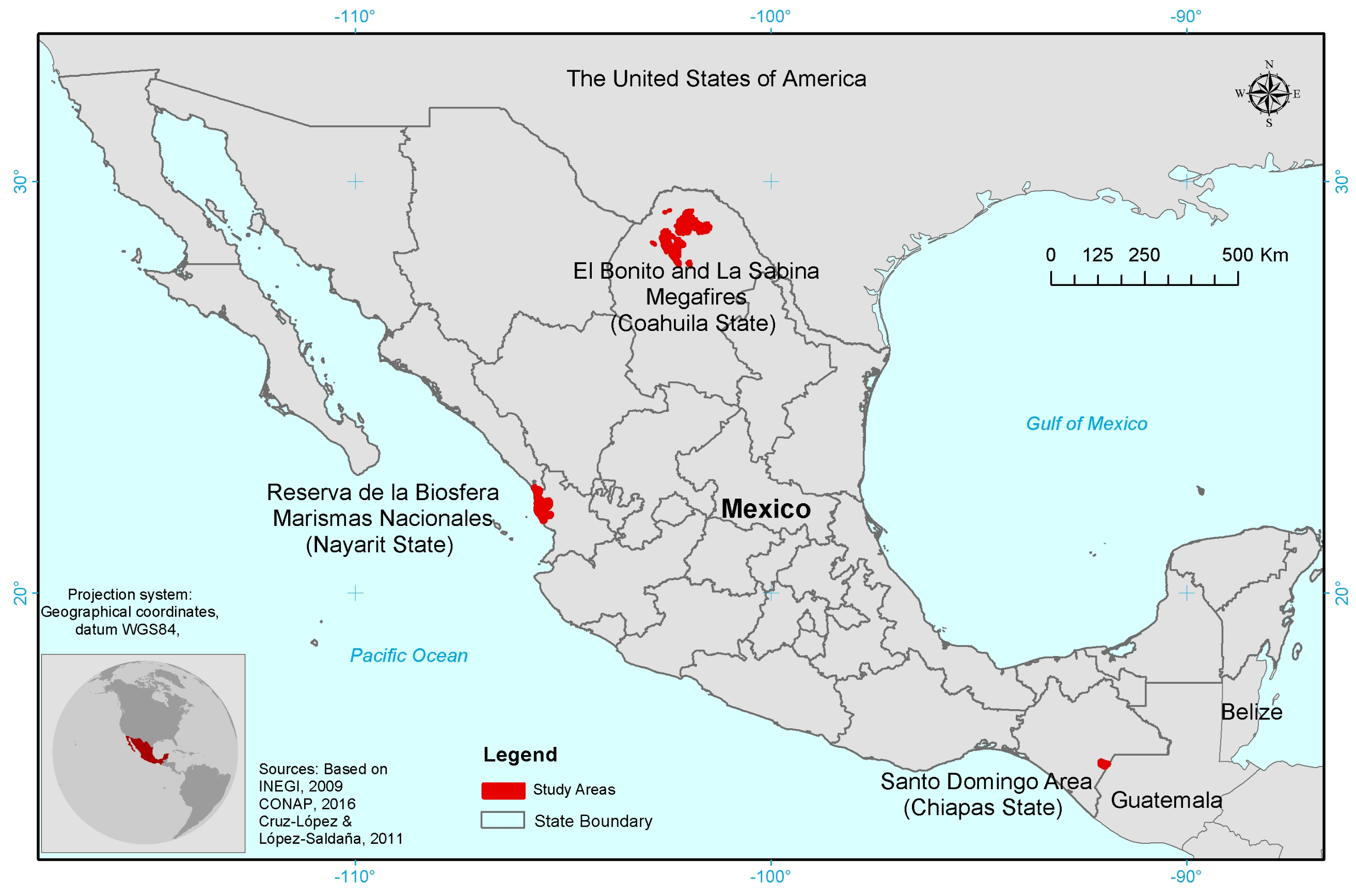
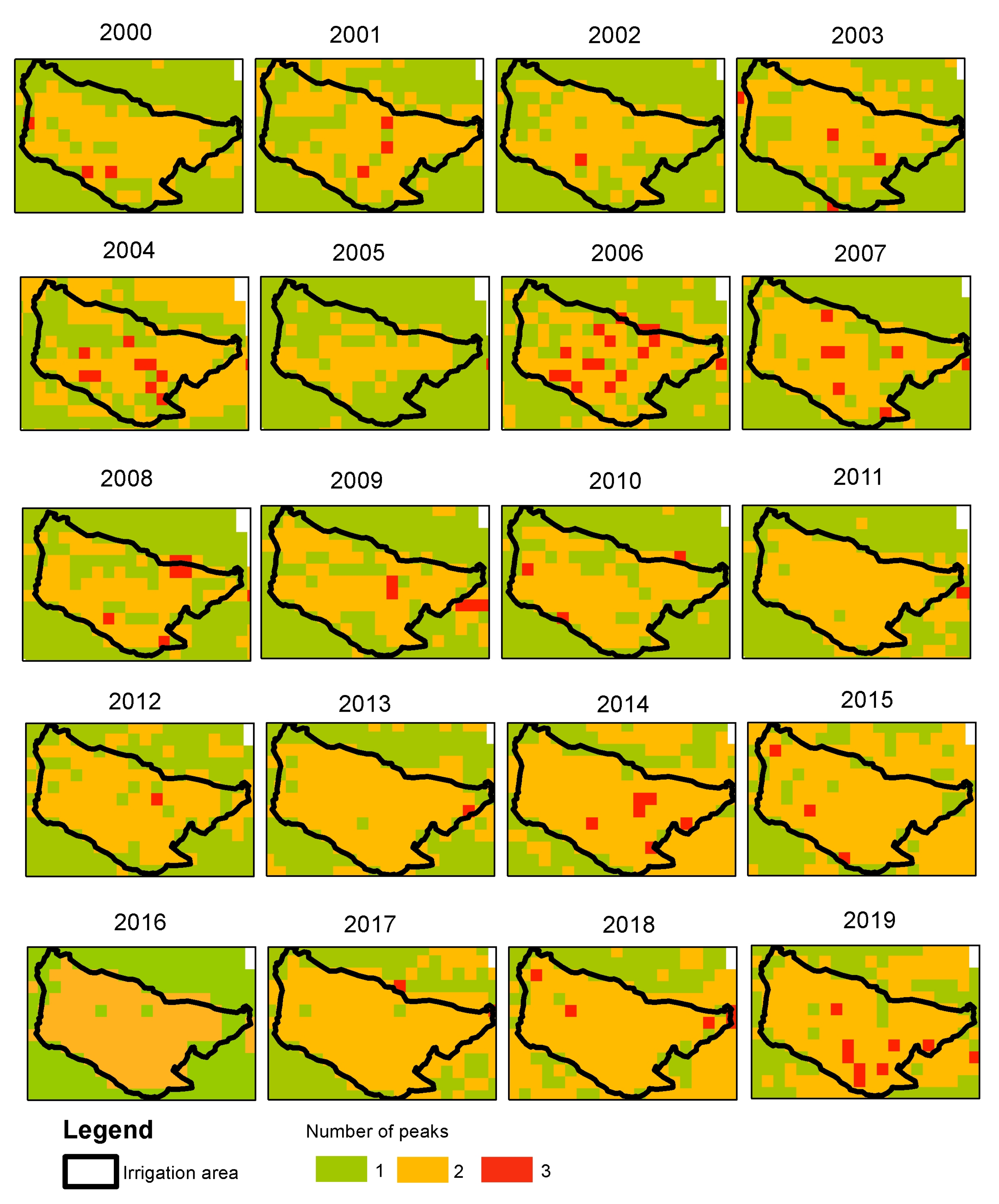
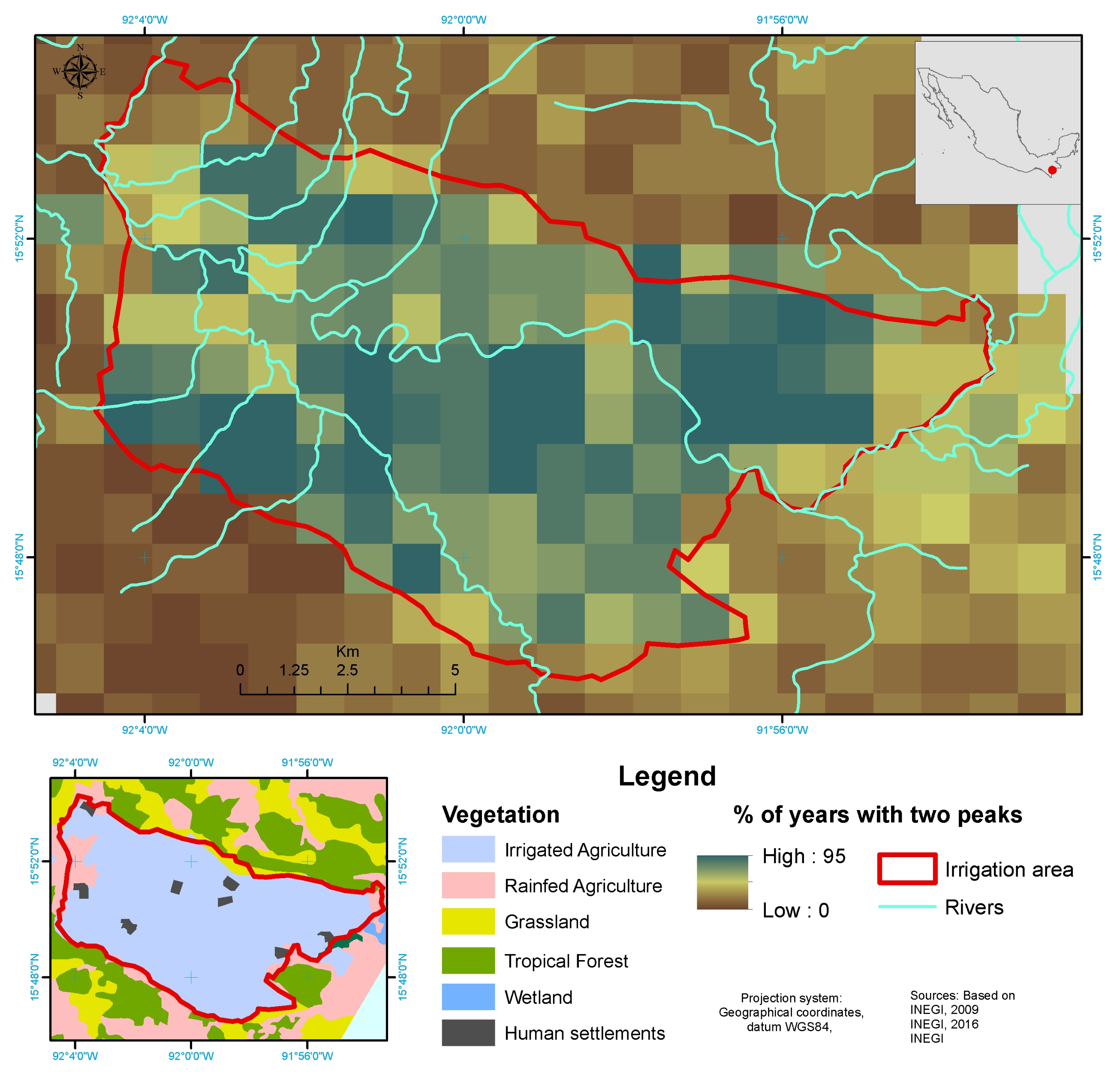
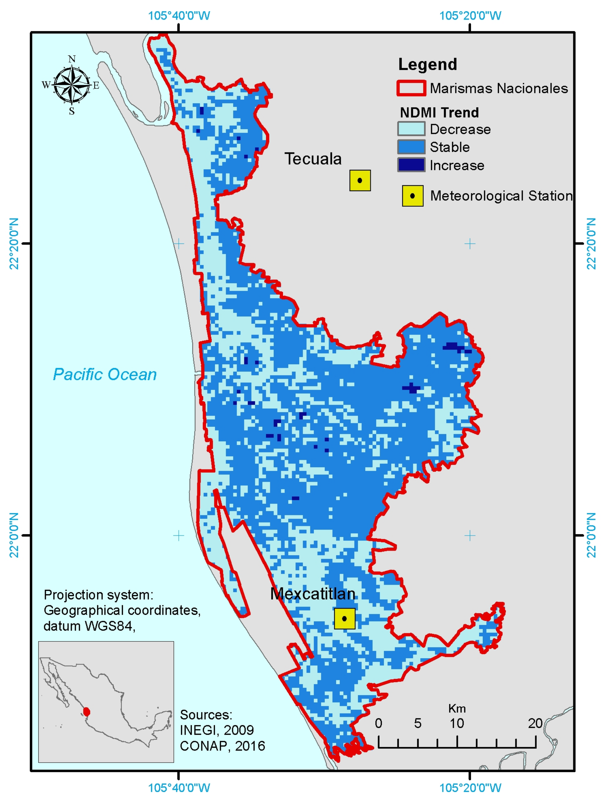
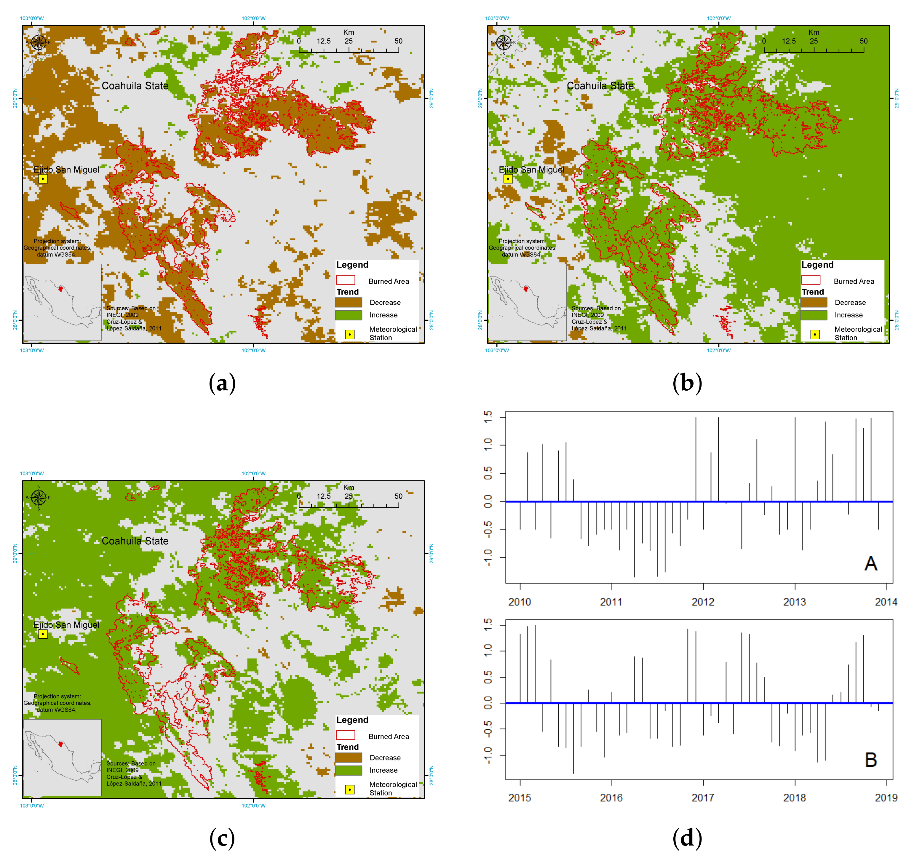
Section 3, we present three illustrative examples of using TATSSI with MODIS data to: (1) assess spatio-temporal changes within an irrigation area, (2) perform a trend analysis of a moisture index in a wetland ecosystem and (3) monitor vegetation in a burned area. Section 4 provides a summary of some of TATSSI’s methods for handling and analyzing EO time series, Section 5 discusses the results of our applications, and finally, Section 6 presents a conclusion and an outlook for future research.

2. TATSSI: Tools for Analyzing Time Series of Satellite Imagery

  In this section we discuss TATSSI’s architecture, design and allowed file formats, as well as how a quality assessment can be carried out, and why by allowing three application programmed interfaces (APIs), this EO data platform is exceptionally user-friendly.

2.1. Architecture and Design

The first stage of any scientific software development project must include gathering user requirements. The main goal of the National Council of Science and Technology (CONACYT, in Spanish) funded project “Statistical Analysis of Time Series of Satellite Imagery with respect to Desertification Processes in Mexico” was to provide a software tool that would allow for monitoring desertification processes by analyzing time series of satellite images. However, providing these kinds of capabilities can be seen as a requirement for a generic toolbox. The toolbox should provide users the functionalities to create and analyze EO products with some insights into remote sensing and statistical analysis. The initial user requirements provided useful insights about the main goals that needed to be addressed within the scope of the project. Five key elements were identified: (i) data discovery and the downloading of coarse and high resolution data; (ii) generation of time series, wherein quality assessment and quality control are taken into account; (iii) interpolation and smoothing of time series; (iv) time series analysis to identify and quantify trends and changes over time; and (v) the use of different interfaces. TATSSI’s design aims at a modular structure in which each component has specific objectives. Figure 1 graphically shows the three main components we identified to create a simple 3-layered architecture. All components will be described in the following subsections.

2.2. Data Handling

  TATSSI aims to provide data discovery and the ability to download coarse resolution data from multiple online Earth Observation (EO) data discovery portals, for which we selected the Application for Extracting and Exploring Analysis Ready Samples (A ρ ρ EEARS) [36] application programming interface (API), which allows submitting and downloading A ρ ρ EEARS requests using the command line or within programming languages such as Python and R. The A ρ ρ EEARS API complies with representational state transfer (REST) principles, and therefore has predictable resource-oriented URLs and uses HTTP response codes showing the status of the corresponding API call. TATSSI uses the product search capability within A ρ ρ EEARS API; this requires user authentication that is stored as a TATSSI config file. When TATSSI is started for the very first time, the A ρ ρ EEARS API is used to create a data catalog containing all MODIS and VIIRS data products available for download from the NASA EOSDIS Land Processes Distributed Active Archive Center (LP DAAC). The catalog is stored in a Python pickle for further use. If there are any changes in the product availability, metadata or versions, the catalog can be rebuilt at any time. TATSSI uses the default MODIS Sinusoidal Grid to get the data by tiles. Additionally to the LP DAAC, TATSSI allows acquiring data from GEE, in which case the data can be acquired for a user-defined area of interest. To obtain the data, the user must have valid Google credentials. In Section 2.4 we provide an example of how this task can be carried out.
Initially, TATSSI rely on a data processing approach through downloaded data stored in local resources, such as network area storage (NAS), local hard drives or storage attached to a VM. This approach allows full customization of the processing flow to create time series that are fit for purpose in terms of scientific applications. Once the data are downloaded, time series can be created. TATSSI can generate a time series for any MODIS and VIIRS dataset obtained from the LP DAAC, but it is possible to use some of TATSSI functionalities for time series not created with TATSSI. As an example, in Section 2.5 we showed how to integrate some Landsat data into TATSSI’s workflow. The metadata in those files allow access to each scientific dataset (SDS) and their corresponding quality assessment (QA) and quality control (QC) flags. The QA/QC flags are only decoded during the time series generation process, their further processing being detailed in Section 3. TATSSI uses Cloud Optimized GeoTIFF (COG) as its internal data format. A COG is a regular GeoTIFF file that can be hosted on an HTTP file server and has an internal organization by chunks, which allows an efficient workflow since a request will ask for just the parts of the needed file. The default behavior when generating a time series is:
  • For every file in the data directory that matches the product and version selected by the user:
    Each band or SDS is imported in the internal TATSSI format (COG).
  • For each QA layer associated with the product:
    Import data into the internal TATSSI format and perform the QA decoding for each flag.
  • For each SDS and associated QA/QC:
    Generate GDAL VRT layer stacks
MODIS and VIIRS data acquired on the LP DAAC are distributed in two different Hierarchical Data Format (HDF) modalities: HDF4 (4.x and previous releases) and HDF5. These formats are not compatible with each other because of their intrinsic differences. TATSSI uses the Geospatial Data Abstraction Library (GDAL) [30] to process data from both sensors. NASA’s Earth Observing System (EOS) maintains its own HDF modification named HDF-EOS. This modification is adequate for use with remote sensing data and fully compatible with underlying HDF. TATSSI uses the GDAL HDF driver to handle all MODIS data. For handling VIIRS data distributed in the HDF5, TATSSI uses the GDAL HDF5 driver; however, geolocation information is not read by default by GDAL (version 2.03.030), for which additional functionality was required to obtain the spatial reference system and geographical extent. In terms of data products generated by TATSSI, the default format is COG, but it is possible to generate output files in several of the formats supported by GDAL, including standard GeoTiff, NetCDF and generic binary.

2.3. Engine

  The TATSSI engine component, as shown in Figure 1, consists of several sub-components, allowing us to: (i) perform an exhaustive analysis of the quality information and creation of an interpolated time series that incorporates the knowledge of the QA/QC, (ii) smooth time series and (iii) apply various methods to analyze time series. A thorough analysis of the characteristics of any EO data product is required to make a consistent interpretation of the data. This analysis can start with the data type and bit depth that can be associated with radiometric resolution. The analysis can continue with the corresponding scaling and offset factors, followed by the identification of the per-pixel QA/QC flags. Some datasets provide quantitative data on top of the QA/QC information in the form of per-pixel uncertainties, or even full variance-covariance matrices, as in the the GlobAlbedo dataset [37]. MODIS and VIIRS land datasets use a consistent QA framework developed by the MODIS Land (MODLAND) Science Team (ST) [38]. The MODLAND QA products provide product-specific QA flags together with metadata that allow traceability along the processing chain. Per-pixel QA data can differ considerably among products, processing levels and collections. Additionally, some products provide different ancillary datasets used during QA generation, which might include atmospheric state, surface type, acquisition geometries, and whether a priori or dynamic atmospheric estimates were used during the biophysical retrieval. In this regard, TATSSI’s main challenge was to be able to access all QA related information for any product distributed by the LP DAAC. TATSSI takes advantage of the per-product quality information distributed on the A ρ ρ EEARS API (https://lpdaacsvc.cr.usgs.gov/services/appeears-api/) (accessed on 16 April 2021) to create a catalog with all products and associated QA/QC definitions (parameters, description, bit fields and values). MODIS and VIIRS QA information is stored as an integer value that needs to be decoded into binary strings. QA/QC decoding takes place by interpreting the binary string, extracting bit words for different bit fields and mapping that unique combination to quality attributes associated with each field. Table 1 shows an example of the first two-bit fields [0–1] from the MOD13A2 "1_km_16_days_VI_Quality” product. The integer value is converted into binary, and then bit fields 0 and 1 are extracted to create a bit word which afterwards is converted into decimal. TATSSI will create a layer for each QA parameter associated with that QA SDS in a way that the user can simply select which QA parameters and values will be selected and flagged as valid for further processing.
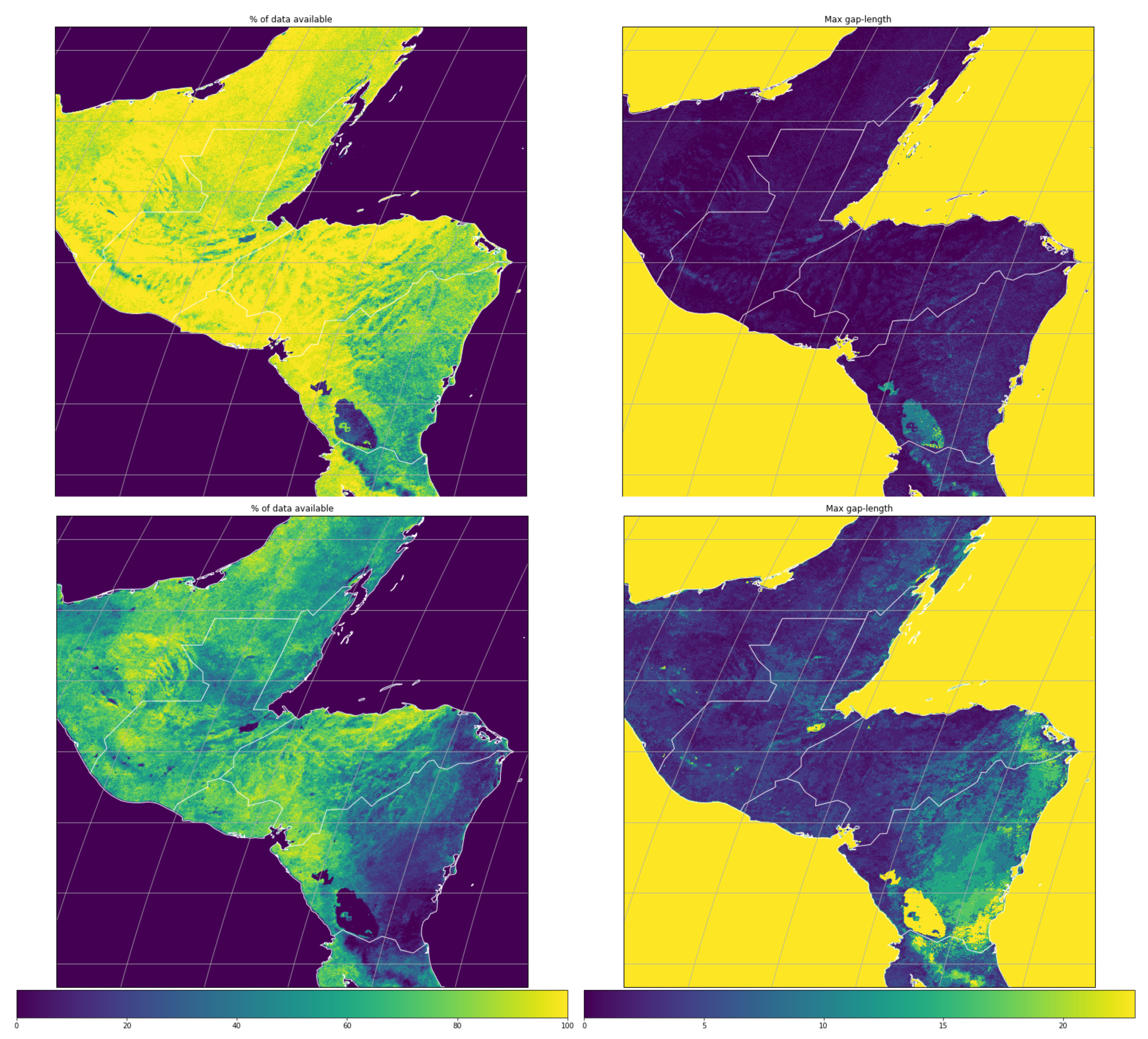
Once the user has selected potential QA parameters and values for a specific SDS, TATSSI will apply that selection to the whole time series to create a mask of valid pixels. The impact of the selection in terms of (i) the percentage of data kept for further processing and (ii) the maximum gap length, can be quantified as the number of missing observations. These metrics can be used to assess the impacts of using different QA settings. Figure 2 shows an example of using the best data with high confidence or some more lenient QA values. The metrics were generated for the MODLAND parameters on the “1_km_16_days_pixel_reliability” layer from the MOD13A2 product. The metrics for the “Good data, use with confidence” QA values in the bottom row in Figure 2 show that the proportion of data available for the eastern region of Lake Nicaragua was below 20%, and the maximum gap length was greater than 20. Since the MOD13A2 provides observations every 16 days, 23 observations fall within one calendar year, meaning that there were almost no observations left after applying the most strict QA value. When using the “Marginal data. Useful but look at other QA information” QA value, the increases in the percentage of data available and the maximum gap length became evident. The TATSSI QA Analytics module allows us to assess different QA settings in a systematic way, so users can select the most adequate set according to their particular needs. The trade-off will be always to keep the best quality data while still fully characterizing the environmental processes of interest. Stricter QA selection results in less availability. If the data gaps produced due to this strict selection occur during a key moment during the seasonality of the studied variable, this may lead to potential misunderstandings or spurious findings, for example, the start and peak of the vegetation season. A more lenient QA selection could easily lead to lack of data to the point where it becomes impossible to understand the environmental variable of interest, as is shown in Figure 2 for Southern Nicaragua. The worst case scenario is applying no QA at all and drawing conclusions based on potential low quality retrievals or observations, as shown by Schaaf et al. [25].
The mask generated during the QA Analyticsprocess is used in the next stage, where different interpolation methods can be applied to generate a gap-free time series, and finally, if required, the user can apply a smoothing function to the time series. The interpolation and smoothing methods are detailed in Section 4. It is important to note though that the TATSSI smoothing process performs a robust outlier detection that could minimize the use of more lenient QA settings, allowing more low-quality observations to be included in the time series, but removing them during the process. By having a gap-free time series, obtained either by interpolation or smoothing, it is possible to subsequently use the TATSSI Time Series module to apply a wide range of statistical techniques and time series operations to extract information and metrics from the time series. These operations and analysis vary from the derivation of the so-called climatology curve and the calculation of per-time-step anomalies, to performing statistical trend analysis, time series decomposition and change point detection. Products for every analysis are stored in COG format. Details about algorithms and techniques used are described in Section 4. If the user needs to ingest a time series that was not generated using the TATSSI processing chain, additional metadata are required to allow the Analysis module to read dates and fill values; we present such an example in the next section.

2.4. Interfaces

  Access to TATSSI functionalities can be chosen depending on the complexity of the task, the amount of data to process and the software development expertise. TATSSI provides three APIs: (i) native GUI, (ii) Jupyter Notebooks and (iii) command line and Python scripting. The GUI was developed using PyQT5, which allows a seamless use of native Python and Matplotlib [39] to generate interactive plots, a key functionality within the TATSSI GUI. 
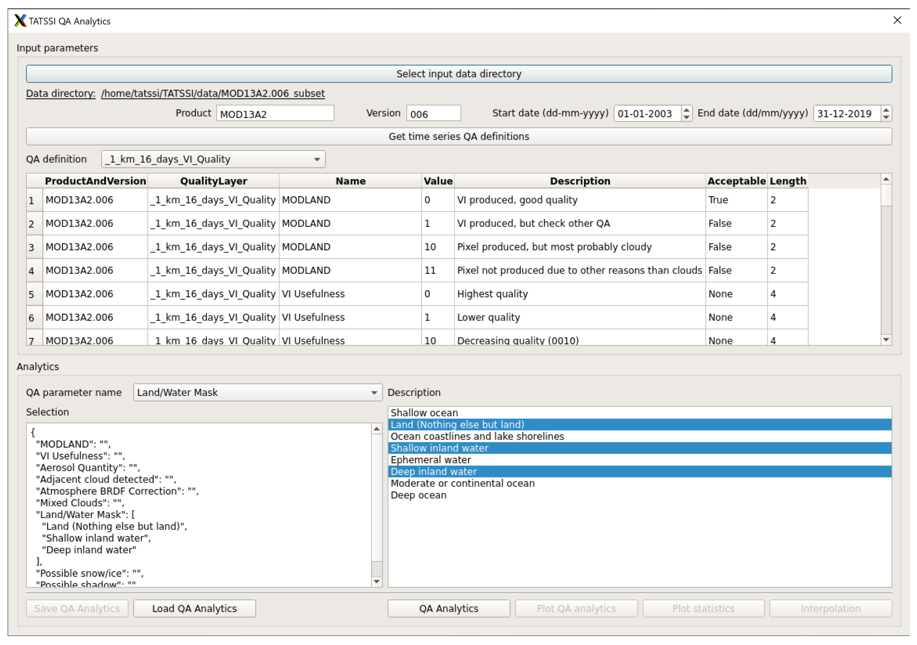
Figure 3 illustrates an example of the TATSSI GUI QA Analytics module. The dialog allows us to perform QA Analytics, as described in Section 2.3. We used a combination of multiple PyQT5 elements to allow the user to open a command dialog to select the location of a time series; write text for products and version; and select dates and QA definitions. Additionally, for every QA parameter, the application of PyQT5 elements allows us to select and unselect desired QA values. We also provided PyQT5 push buttons for the user to access different dialogue boxes.
Jupyter Notebook [40] is an open-source web application that allows the creation of interactive documents that contain live code, visualizations and narrative text. TATSSI provides several Notebooks as a step-by-step guide to understand the different TATSSI functionalities in a similar fashion as when using the GUI, but executed from a web browser. TATSSI supports JupyterLab, the next-generation version of the web-based interface. The main advantage of this interface is that there is no need to install any software on the client side. The Jupyter Notebooks can be executed either locally, for example, on a local workstation, or remotely, for example, on a cloud computing VM. When the Jupyter Notebooks are executed remotely, as in a cloud environment, the data processing can be executed as a background process. This means that the user does not need an active connection to the cloud environment. This feature provides an alternative to launching jobs and retrieving the results afterwards.
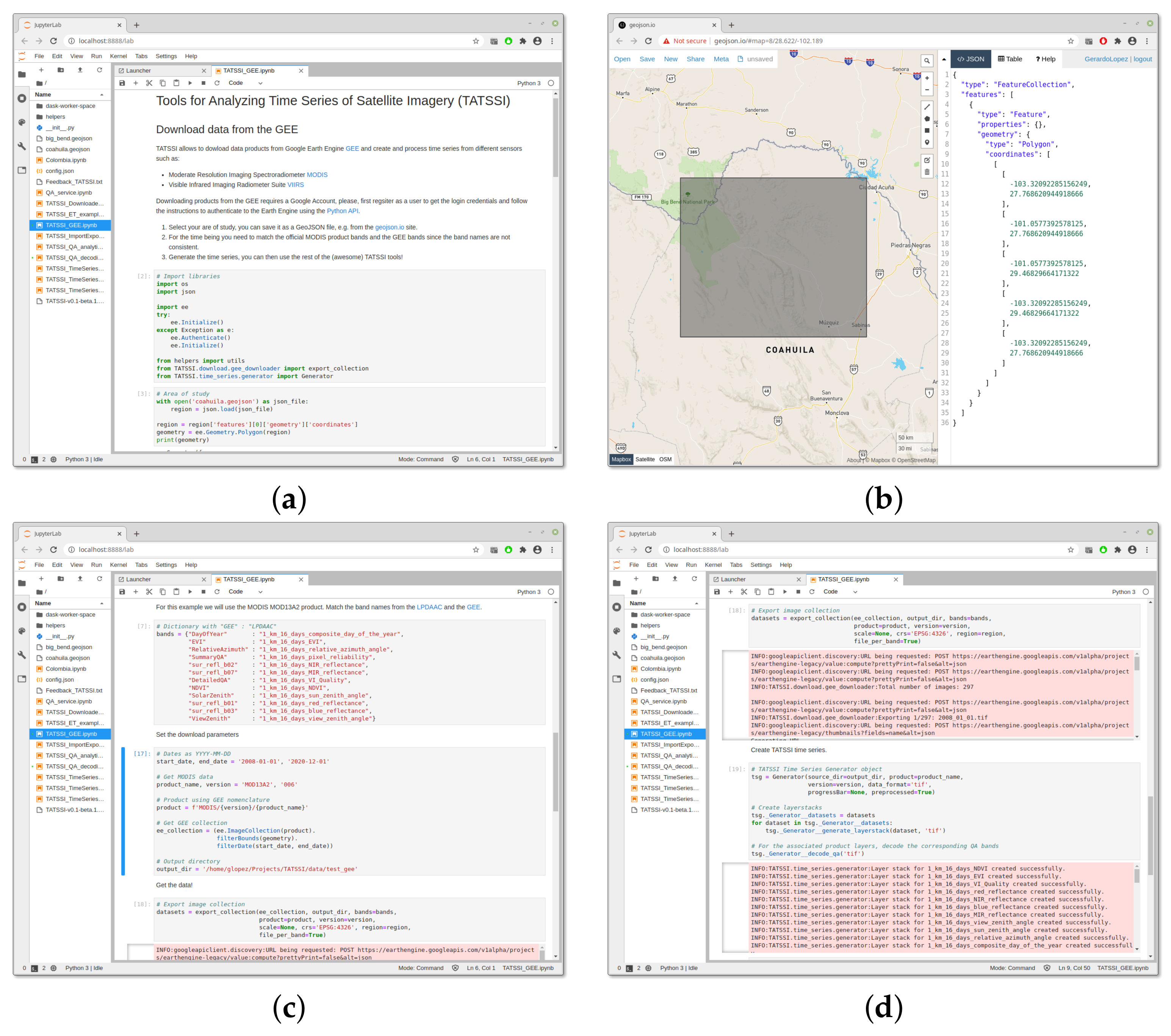
Figure 4 illustrates an example of the use of a Jupyter Notebook in TATSSI, a particularly useful feature when the area of interest (AOI) is divided amongst two or more MODIS tiles. The first step is setting Google Earth Engine (GEE) authentication and importing the required TATSSI libraries, as in Figure 4a, after which the user must define an AOI as a bounding box that is subsequently saved into a GeoJSON file. Figure 4b shows the AOI defined for one of our study sites in northern Mexico (see Section 3.3 for further details). An important step is to match the SDS names from the GEE and the ones from MODIS datasets. The product layers names for some of the products available within the GEE must be modified to apply the corresponding QA flags using the metadata available from the TATSSI catalog, as we show in Figure 4c. The final step is downloading the data and generating the time series (Figure 4d). The time series thus generated can afterward be used for further processing in the TATSSI modules of interest.
For users familiarized with Python, TATSSI provides modules that can be called from a script, as is shown in the following example to generate a time series. The user needs to import the corresponding TATSSI module in Python (e.g., Generator); set input parameters such as source directory, product and version and input data format; create the time series Generator object; and finally, call the generate_time_series() method, see Listings 1.
Listing 1. Python script used by TATSSI to generate time series.
# Import TATSSI modules   
from TATSSI.time_series.generator import Generator
             
# Set downloading parameters
source_dir = ‘/data/MCD43A4_h08v06’
product = ‘MCD43A4’
version = ‘006’
data_format = ‘hdf’
             
# Create TATSSI the~time series generator object
tsg = Generator(source_dir=source_dir,
                product=product, version=version,
                data_format=data_format)
             
# Generate the~time series
tsg.generate_time_series()
As mentioned above, TATSSI stores all geospatial raster data as COGs. To perform any time series operation and analysis, TATSSI loads the time series as xarrays [41]. xarray is a Python package that works by accessing multi-dimensional arrays in a very efficient way by introducing labels on top of raw NumPy [42] arrays in the form of dimensions, coordinates and attributes. Additionally, xarray provides full integration with DASK for parallel computing. By applying the code above to the MCD43A4 time series generated from the MODIS tile h08v06, it is then possible to load the TATSSI time series object as an xarray for further processing. Listings 2 provides an example of computing and storing the normalized difference moisture index (NDMI), utilized in Section 3.2:
Listing 2. Calculation of Normalized Difference Moisture Index based on the MCD43A4 product taken on tile h08v06.
import os
import sys
             
# TATSSI modules   
from TATSSI.time_series.analysis import Analysis
from TATSSI.input_output.utils import save_dask_array
             
# TATSSI time series object for band 2
fname = (f‘/data/MCD43A4_h08v06/Nadir_Reflectance_Band2/’   
         f‘interpolated/MCD43A4.006._Nadir_Reflectance_Band2.linear.tif’)
ts_b2 = Analysis(fname=fname)
# Get DataArray from {\tatssi} time series object
b2 = ts_b2.data._Nadir_Reflectance_Band2
             
# TATSSI time series object for band 6
fname = (f‘/data/MCD43A4_h08v06/Nadir_Reflectance_Band6/’
         f‘interpolated/MCD43A4.006._Nadir_Reflectance_Band6.linear.tif’)
ts_b6 = Analysis(fname=fname)
# Get DataArray from {\tatssi} time series object
b6 = ts_b6.data._Nadir_Reflectance_Band6
             
# Compute normalized difference moisture index (NDMI)
ndmi = ((b2-b6) / (b2+b6)).astype(np.float32)
             
# Copy metadata attributes from band 2
ndmi.attrs = b2.attrs
# Change fill value to 0
ndmi.attrs[‘nodatavals’] = tuple(np.zeros(len(ndmi.time)))
             
# Save data
fname = ‘/data/marismas_NDMI.tif’
data_var=‘NDMI’
             
save_dask_array(fname=fname, data=ndmi, data_var=data_var)

2.5. Adding Metadata to EO Time Series Not Generated by TATSSI

One of the main purposes of using TATSSI is to genere a time series utilizing the associated QA/QC information provided. However, if the user already has a time series generated using other time series tools but still wants to use TATSSI for further analysis, date, variable description and fill value metadata must be added to every band in the time series, which will allow the different TATSSI interfaces to read the time series, and for example, perform smoothing or use the Analysis module. Listings 3 shows how to add metadata to Landsat 7 surface reflectance:
Listing 3. Python script to add metadata to Landsat 7 images.
import os
import sys
import gdal
from glob import glob
import datetime as dt
              
DataDir = ’/data/Landsat7’
              
def add_metadata(fname, str_date, data_var, fill_value):
    """
    Adds date to metadata as follows:
        RANGEBEGINNINGDATE=YYYY-MM-DD
    :param fname: Full path of files to add date to its metadata
    :param str_date: date in string format, layout: YYYY-MM-DD
    :param data_var: Variable name, e.g. surface_reflectance
    :param fill_value: Fill value
    """
             
    # Open the file for update
             
    d = gdal.Open(fname, gdal.GA_Update)
             
    # Open band and get existing metadata
    md = d.GetMetadata()
             
    # Add date
    md[’RANGEBEGINNINGDATE’] = str_date
    # Add variable description
    md[’data_var’] = data_var
    # Add fill value
    md[’_FillValue’] = fill_value
             
    # Set metadata
    d.SetMetadata(md)
             
    d = None
             
if __name__ == "__main__":
             
    # Get all file from data directory for Landsat band 4, for instance
	# /data/Landsat7/LE70290462004017EDC01/LE70290462004017EDC01_sr_band4.tif
    fnames = glob(os.path.join(DataDir, ‘*’, ‘*_sr_band4.tif’))
    fnames.sort()
             
    for fname in fnames:
        # Extract date from filename
        # LE7PPPRRRYYYYDDDEDC01_sr_band4.tif
        # YYYY = year
        # DDD = julian day
        year_julian_day = os.path.basename(fname)[9:16]
             
        # Convert string YYYYDDD into a datetime object
        _date = dt.datetime.strptime(year_julian_day, ‘%Y%j’)
        # Convert datetime object to string YYYY-MM-DD
        str_date = _date.strftime(‘%Y-%m-%d’)
             
        # Set data variable to a descriptive ’L7_SurfaceReflectance_B4’
        data_var = ‘L7_SurfaceReflectance_B4’
             
        # Add metadata
        add_metadata(fname=fname, str_date=str_date,
                data_var=data_var, fill_value=‘-9999’)
Once the metadata have been stored in every file and band, it is possible to create a GDAL virtual raster that TATSSI can read, see Listings 4.
Listing 4. Creating a GDAL Virtual Raster from files modified through Listings 3’s code.
gdalbuildvrt -separate LE70290462004.vrt /data/Landsat7/*/*_sr_band4.tif
0...10...20...30...40...50...60...70...80...90...100 - done.
After that, it is possible to open the Landsat 7 VRT with any TATSSI interface, as Figure 5 shows for the Smoothing module for the Landsat 7 near-infrared (NIR) band time series during 2004.

2.6. Cloud Computing Environments

  The previous section presented TATSSI’s capabilities regarding data being downloaded and subsequently used to generate a time series. Nevertheless, the paradigm of processing EO data using local resources may not be computationally efficient for all use-cases, e.g., a data server with attached storage or high-end workstations where vast amounts of data need to be transferred from a data provider. Gomes et al. [34] defined “Platforms for big EO Data Management and Analysis" as computational solutions that provide functionalities for big EO data management, storage and access that provide certain level of data and processing abstractions. In this context, TATSSI provides some features that can be exploited in cloud computing and high-performance computing environments.
TATSSI can be used on a cloud environment where one or more VM can be created and multiple users can access the resources. This can be seen as a hybrid paradigm because the EO data have to be downloaded to local storage within the VM, allowing different users to create time series without using local resources; thus, data are processed and stored on the server side.
The TATSSI approach encourages users to fully understand the limitations and constraints of each dataset, including the associated QA and QC flags. This understanding might require to download and analyze the data. It is expected that some abstraction is required to maximize the use and exploitation of EO data. This hybrid cloud computing approach can be attractive to users with some existing knowledge of EO data but requires some data abstraction; e.g., details about how raw data are stored, compression algorithms and metadata are not necessarily relevant.
When some processing abstraction is required and a processing chain is well-defined, downloading data, even to cloud storage, is not viable. TATSSI takes advantage of the GDAL Virtual File Systems where files stored on a network (either publicly accessible, or in private buckets of commercial cloud storage services) can be accessed. For instance, MODIS product MCD43A4 v006 Nadir Bidirectional Reflectance Distribution Function (BRDF)-Adjusted Reflectance (NBAR) for 3 March 2021 in COG format stored on a commercial cloud storage that does not require signed authentication can be accessed from the command line, see Listings 5.
Listing 5. Accessing to MCD43A4 products stored on a cloud facility.
gdalinfo-nomd/vsicurl/https://modis-pds.s3.amazonaws.com/MCD43A4.006/18/17/2021062/MCD43A4.A2021062.h18v17.006.2021071072416_B02.TIF
Driver: GTiff/GeoTIFF
Files: /vsicurl/https://modis-pds.s3.amazonaws.com/MCD43A4.006/18/17/2021062/MCD43A4.A2021062.h18v17.006.2021071072416_B02.TIF
       /vsicurl/https://modis-pds.s3.amazonaws.com/MCD43A4.006/18/17/2021062/MCD43A4.A2021062.h18v17.006.2021071072416_B02.TIF.ovr
Size is 2400, 2400
Coordinate System is:
PROJCS["unnamed",
    GEOGCS["Unknown datum based upon~the~custom spheroid",
        DATUM["Not_specified_based_on_custom_spheroid",
            SPHEROID["Custom spheroid",6371007.181,0]],
        PRIMEM["Greenwich",0],
        UNIT["degree",0.0174532925199433]],
    PROJECTION["Sinusoidal"],
    PARAMETER["longitude_of_center",0],
    PARAMETER["false_easting",0],
    PARAMETER["false_northing",0],
    UNIT["metre",1,
        AUTHORITY["EPSG","9001"]]]
Origin = (0.000000000000000,-8895604.157332999631763)
Pixel Size = (463.312716527916677,-463.312716527916507)
Corner Coordinates:
Upper Left  (       0.000,-8895604.157) (  0d 0‘ 0.01"E, 80d 0’ 0.00"S)   
Lower Left  (       0.000,-10007554.677) (  0d 0’ 0.01"E, 90d 0’ 0.00"S)   
Upper Right ( 1111950.520,-8895604.157) ( 57d35’15.74"E, 80d 0’ 0.00"S)
Lower Right ( 1111950.520,-10007554.677) ( 46d55‘34.78"E, 90d 0’ 0.00"S)   
Center      ( 555975.260,-9451579.417) ( 57d22’ 6.84"E, 85d 0’ 0.00"S)   
Band 1 Block=512x512 Type=Int16, ColorInterp=Gray
  Description = Nadir_Reflectance_Band2
  NoData Value=32767
  Overviews: 1200x1200, 600x600, 300x300
  Offset: 0,   Scale:0.0001
This allows TATSSI to access files stored on cloud storage and generate time series using the approaches and interfaces mentioned in this section.

3. Study Sites and Materials

  TATSSI can be used as an effective tool for generating QA-based EO time series and conducting basic statistical analysis. In Section 5, we will show applications for three case studies: irrigation area changes (IA) in Santo Domingo, southern Mexico; evaluation of moisture dynamics (EMD) in the wetland ecosystem Marismas Nacionales, Mexican Pacific; and burned area monitoring (BAM) at El Bonito and La Sabina, northeastern, Mexico. In the following section we describe the study sites, comment on the MODIS products employed in each study and discuss some materials used to complement our analysis. Following that, we will describe data pre-processing in Section 3.4.

3.1. Irrigation Area Changes in Santo Domingo

The vegetation indices are used to monitor vegetation, crop production and other processes [43]. A time series of vegetation index provides information to identify land-cover or land-use changes [20]. A change in the vegetation index behavior can be an indicator of land cover change from natural to anthropogenic cover, or it can also indicate a change in agriculture practices. That is the case for the Santo Domingo Area—in the state of Chiapas, southern Mexico—located between La Angostura dam and the border with Guatemala with an extension of 15,147 ha (Figure 6). The area is crossed by the rivers Santo Domingo and San Gregorio, both tributaries of the Grijalva River System. Originally, the land cover was tropical dry forest; then it became rainfed agriculture; and at present it is irrigated agriculture surrounded by some patches of tropical dry forest.
We studied these land cover changes in the Santo Domingo Area through analyzing the frequencies of maxima (peaks per year) and minima (valleys over year) of the enhanced vegetation index (EVI) from the MOD13A2.006 product during the period 2001–2019. We used thematic cartography to verify the land cover in the area. Additionally, we consulted six land-use and vegetation maps (with 1:250,000 cartographic scale) elaborated by the Instituto Nacional de Estadística y Geografía (INEGI) and released in 1980, 1993, 2002, 2007, 2011 and 2014.

3.2. Evaluation of Moisture Dynamics of Marismas Nacionales

  Wetlands are rich in biodiversity and provide ecosystem services such as fish production and carbon sequestration [44,45,46,47]. Their preservation is necessary to control many natural processes, such as flooding [48]. Wetlands are very dynamic [49] and humidity monitoring is an effective tool to evaluate this dynamic. We chose the Natural Protected Area (NPA) Reserva de la Biosfera Marismas Nacionales to analyze moisture dynamics. Marismas Nacionales is one of the most relevant wetland systems on the Mexican Pacific coast. In this area, diverse ecosystems are represented, such as halophilous vegetation, tropical dry forest, thorn shrubland, coastal dune vegetation, estuaries, lagoons, marshes and mangroves [50]. Marismas Nacionales is located within five counties in the state of Nayarit, Western Mexico (Figure 6), and its area covers 133,854 ha [51].
We studied the moisture dynamics of Marismas Nacionales through trend analysis of a time series of the normalized difference moisture index (NDMI), which according to Wilson and Sader [52] is an appropriate variable for our purpose. We derived our NDMI time series from the MCD43A4 daily product for the period 2015–2018. After pre-processing, we obtained an interpolated time series of 1461 MCD43A4 images. We employed the MCD43A4’s near-infrared (NIR) and mid-infrared (MIR) bands to compute the NDMI as follows: N D M I = ( N I R M I R ) / ( N I R + M I R ) . As an effective temporal aggregation method that preserves the main features of moisture dynamics, we calculated the arithmetic mean of NDMI values within a 10-day period. For the latter two steps, we developed a Python script. The final 10-day NDMI composite time series that we analyzed consisted of 37 observations per year. Additionally, we used records of the meteorological stations Mexcaltitán (located at the southern part of the NPA Marismas Nacionales) and Tecuala (at the northern border of the NPA) to obtain the time series of daily precipitation and maximum and minimum temperature from 2015 to 2018. Since these auxiliary data were employed to compare the findings of our trend analysis of the NDMI time series, we adjusted the records to match the same temporal scale as the NDMI time series. Namely, we computed 10-day composites of precipitation and temperature by adding the  precipitation values within a 10-day period, and computing the arithmetic mean of the temperature variables.

3.3. Burned Area Monitoring at El Bonito and La Sabina

  2011 was a dry year in Mexico in which two megafires were registered on El Bonito and La Sabina in the Serranias del Burro mountain range located in the state of Coahuila in northern Mexico, both affecting 355,425 ha of oak forest, oak-pine forest, chaparral and piedmont shrubland, desertic rosetophyllous shrubland and natural grassland [53]. These fires persisted from March to May 2011. The apparent drought in the area, registered since the second half of 2010, may have triggered these fires and fueled its drastic behavior [54]. The drought affected the whole area; this is the reason we studied this case analyzing vegetation index behavior in and outside of the burned area.
We studied the vegetation changes by analyzing the EVI layer of the MOD13A2.006 product from January 1st, 2008 to October 16th, 2020. Our analysis consisted of a combination of annual change-point decomposition followed by statistical trend analysis at certain periods. The beginning and end of these periods are marked by being the years in which the change-points are spatially more extended. We also studied the drought in the area through the standardized anomalies of a daily precipitation time series from 2008 to 2020 registered in the meteorological station Ejido San Miguel located nearby El Bonito and La Sabina.

3.4. Pre-Processing

Figure 7 shows the TATSSI GUI workflow, including a summary of all of its applications and the parameters required in each step. For pre-processing some of the EO time series used in our applications, we utilized the modules Downloaders, Generator, Analytics, QA Analytics and Interpolation.
  • Download and Time Series Generation. To analyze changes in the irrigation area (IA) of Santo Domingo with TATSSI we focused on the MOD13A2.006’s EVI. The TATSSI GUI Downloaders allowed us to acquire the images of the tile h09v07 from January 1st, 2001 to December 31st, 2019. A further application of the Select Spatial Subset within the Generator module allowed us to define a subset covering the area of interest (AOI). As a reference for our subsetting, we uploaded a shapefile of the AOI via the Geometry Overlay application in the Generator module. To generate the final time series, it is crucial that the original product and the shapefile have the same coordinate reference system and projection. For the EMD case study, we considered the NDMI derived from the MCD43A4 product from which we initially obtained 1461 daily images of tile h08v06 using the TATSSI GUI Downloaders. Then, as for IA, we generated a time series covering the AOI employing Select Spatial Subset and TATSSI GUI Generator modules. Based on this time series, we calculated the NDMI using the Python script presented in Section 2.4 and the details presented in Section 3.2. For the BAM case study, we employed the EVI layer of the MOD13A2.006. The AOI is located on the edge between MODIS tiles h08v06 and h09v06. For an efficient download and generation of the time series to analyze, we combined TATSSI Jupyter Notebook API and the GEE (see Section 2.4 for further details), and acquired subsets of MOD13A2.006 images covering the AOI from 2008 to 2020.
  • Quality assessment and gap-filling. We followed the same QA/QC analysis procedure for IA and BAM using MOD13A2.006’s layer "1_km_16_days_pixel_reliability" with the "Good data, use with confidence" and "Marginal data, Useful, but look at other QA information" flags together. The use of these flags and layers was discussed in Section 2.3. For EMD, the MCD43A4’s quality layer has two flags; we applied the  “Processed, good quality (full BRDF inversions)" layer with the TATSSI GUI Analytics module. After that, the percentage of data available in the time series (per pixel) ranged from 37 to 98%, and the maximum-gap length was between 5 and 153 observations. This lack of information was ameliorated by a subsequent temporal linear interpolation using the Interpolation submodule (within Analytics).

4. Methods

In addition to downloading and generating time series incorporating scientific datasets with quality assessment, TATSSI allows interpolation, smoothing and performing basic statistical analysis with EO time series. In this section we briefly describe these procedures.

4.1. Interpolation

TATSSI allows straightforward application of temporal interpolation; no spatio-temporal method is provided. We believe that linear, nearest and spline temporal interpolation are in line with the spirit of providing basic tools for data analysis, in this case for gap-filling data. The TATSSI GUI also provides a set of graphical panels (two maps and a plot area) in which the user can select any of the interpolation methods and apply it to a time series, and by clicking on any of the maps, the user can select a different time series (pixel). Since it is possible to apply the three interpolation methods at once, this tool may help users to decide on the interpolation methods to fit their purposes. In our applications (IA, EMD and BAM) we opted for temporal linear interpolation as a gap-filling method. The linear, nearest and spline interpolation methods of TATSSI are applications of the numpy interpolation, inter1d and scipy.interpolate libraries of Python, respectively.

4.2. Standard Anomalies

TATSSI calculates standard anomalies as follows. For a time series ( X i ) i = 1 , , ( P × T ) with P periods (years) and T time-points (observations) in each period, let μ t and σ t be, respectively, the overall mean and standard deviation across the P periods of the time series at a given time-point t:
μ t = 1 P k = 0 P 1 X t + k × T , σ t = 1 P k = 0 P 1 ( X t + k × T μ t ) 2 , t = 1 , , T .
For any time-point t in the period k, the standardized version of X t + k × T is by definition:
A t , k = ( X t + k × T μ t ) / σ t , t = 1 , , T , k = 0 , , P 1 .
TATSSI computes the so-called standardized anomalies based on Equation (1) and displays them in a series of maps (a map for each time-point in the time series). The accompanying consolidated color palette helps users to locate how distant each pixel (multiplied by the corresponding overall standard deviation) is with respect to the overall mean. The standardized anomaly maps can be easily exported in several formats; see Section 2.2.

4.3. Seasonal and Trend Decomposition of Time Series

At the pixel level TATSSI decomposes an EO time series into three independent components (trend, seasonality and residuals) following the classical decomposition model:
X t = T t + S t + e t , t = 1 , , P × T ,
where P and T denote the number of periods (years) and observations per period, respectively.
Let us consider the trend component ( T t in expression above). In this case, the trend estimation is carried out through a moving average with a fixed bandwidth. Although by default TATSSI utilizes the maximum number of observations per period as the bandwidth value, the users are allowed to provide a bandwidth value. If we consider the seasonal component ( S t in expression above), once the trend has been estimated, by T t ^ , we can remove this estimated trend from the original observations forming the so-called detrended time series X t T t ^ . This series is used to estimate the seasonal component. Namely, for a time series with P periods (years) and T time-points (observations) per period, TATSSI uses the following expression to estimate the seasonal component:
S ^ t = 1 P k = 0 P 1 ( X t + k × T T ^ t + k × T ) , t = 1 , , T .
Once trend and seasonal components have been obtained by T ^ t and S ^ t , respectively, the residual component is simply e ^ t = X t T ^ t S ^ t .
We acknowledge the existence of more sophisticated methods for trend and seasonal component estimation. For instance, problem-specific seasonal component estimates can be found in [20,55], among many others. For an exploratory analysis, it may be reasonable to assume that the trend describes a linear structure which can be appropriately estimated through a moving average. Additionally, a simple and effective manner to approximate the seasonal component of the model (2) is through Equation (3). These two basic methods are usually covered in introductory time series analysis textbooks; e.g., Section 1.5.1 of Brockwell and Davis [56]. Thus, we believe that the methods just described are in line with TATSSI’s philosophy. For our burned area monitoring case study—see Section 3.3—we applied the change-point estimation method (described below) to the detrended time series { X t T ^ t } .

4.4. Statistical Trend Analysis

  TATSSI utilizes the Mann–Kendall test to perform trend analysis on EO time series. Briefly, and following [57] and Chapter 4 and 5 in [58], for the time series X 1 , , X n the statistic
S n = i = 1 n 1 j = i + 1 n sign ( X j X i ) ,
where
sign ( X j X i ) = + 1 for   X j X i > 0 1 for   X j X i < 0
can be used to determine whether there exists a trend in the time series; large values of | S n | provide evidence against the null hypothesis of no trend. In order to calculate the p-value of this null hypothesis, it is convenient to utilize the normal approximation of the following statistic:
T n = S n 1 σ n for   S n > 0 S n + 1 σ n for   S n < 0 ,
where
σ n 2 = n ( n 1 ) ( 2 n + 5 ) / 18 .
Let T ^ n be the empirical counterpart of T n . Since we are interested in testing no trend, it is pertinent to employ the two-tailed null hypothesis H 0 : | T n | > | T ^ n | ; the corresponding p-value is equal to 2 P { T n > | T ^ n | } . When p value < α , for some significance level α , then the null hypothesis is rejected; in TATSSI, α = 0.05 is the default significance level for this test. To ease interpretation, the variable trend is defined as follows:
trend = 1 i f H 0 is   rejected   and   T n < 0 0 i f H 0 is   not   rejected   + 1 i f H 0 is   rejected   and   T n > 0 .
As part of TATSSI’s trend analysis, layers (in the GeoTiff format) for T n , p-value and trend are returned. This method was employed to study the NPA Marismas Nacionales moisture dynamics; see Section 3.2 and Section 5.2.

4.5. Change-Point Analysis

Nowadays, there are several methods and pieces of software for performing change-point analysis. In a nutshell, the change-point problem consists of identifying statistically those time-points at which the main characteristics (for instance, mean and standard deviation) of a sequence of observations suffer an abrupt change. Regardless of the procedure to estimate these change-points, it is almost mandatory to account for a computationally efficient implementation of the method.
In TATSSI (within the Analysis module), we developed the application Change-Point Decomposition (CPD). This application is based on the integration of the R package changepoint by Killick and Eckley [59] into TATSSI’s engine. That is, TATSSI begins by executing routines of the R package changepoint and then applies Python’s numpy2ri function to import changepoint’s output from R to Python. A somewhat similar application is the so-called BFAST Explorer of Menini et al. [60].
The changepoint package provides methods to identify changes in mean (cpt.mean), in variance (cpt.var) and in both mean and variance (cpt.meanvar). The contribution of the changepoint package is that, among other things, it allows the user to select among three search change-point methods: segment neighborhood, binary segmentation and Killick et al.’s [61] PELT. Killick and Eckley [59] have described and demonstrated some differences among these procedures. We believe that in the context of analyzing EO time series, our contribution, CPD, consists of providing an interface in which the user can select among three different search methods for estimation of abrupt changes.
For our case study on burned area monitoring (see Section 3.3), we employed cpt.meanvar at the 5% significance level to estimate changes both in mean and variance of the detrended time series of MOD13A2.006’s EVI layer. For this application, we found that binary segmentation was the search method with the best performance.

4.6. Additional Methods for Any Exploratory Analysis of EO Time Series

  • Peaks and valleys. TATSSI’s Analysis module plots the original chosen time series along with its maxima and minima. We also refer to maxima and minima as peaks and valleys, respectively. These peaks and valleys can be exported as a multilayer stack. We analyzed the distribution of these peaks and valleys for our application of irrigation area changes.
  • Smoothing. When in need of a method to remove extra noise and extract an apparent regression signal, TATSSI’s Smoothing module can be used. As shown in Figure 7 this module is in the Time Series menu. This tool is an adaptation of Garcia’s [62] robust smoothing method for massive processing. For our application of irrigation area, before analyzing the distribution of peaks and valleys, we smoothed the EVI time series with a smooth factor of 0.75 .
  • Climatology curve. This curve can be found in a graphical panel of TATSSI’s GUI Analysis module. The user can easily appreciate a series of boxplots (one for each time-point within the time series) highlighting the minimum, 25% quantile, 50% quantile (also known as the median), 75% quantile and maximum of the distribution of the observations (across periods for each time-point). Layers of these statistics, along with layers of mean and standard deviation, can be exported as multilayer stacks.

5. Results

5.1. Distribution of Maximum per Year to Study Irrigation Area Changes

From the TATSSI GUI Analysis module, we obtained a raster stack with the maximum values (peaks) per year in the MOD13A2’s EVI time series from 2001 to 2019. At the pixel level, at any given period/year the EVI time series can have more than one maximum. For instance, two maximum values (peaks) in one year can be linked to two growing seasons. This characteristic can be found in areas under irrigated agriculture. Thus, the ratio of the amount of years with two peaks per year to the total amount of years under consideration is expected to be large in pixels linked to irrigated agriculture. Figure 8 shows the spatial distribution of the ratio just described for the Santo Domingo area. This map allowed us to discriminate pixels in which the EVI reports two peaks per year (pixels with percentage close to 95%) from pixels in which arguably there is at most one peak per season (pixels with percentage below 50%). It is remarkable that the spatial distribution of pixels with one and two peaks coincide with the rivers distribution of the zone. Indeed, according to the vegetation and land use map included in Figure 8, those pixels with a low frequency of two peaks per year can be associated with rainfed agriculture and tropical forest.
According to the vegetation mapping and land use at scale 1:250,000 from the Instituto Nacional de Estadística y Geografía (INEGI) in 1993, the area was characterized as irrigated agriculture. For every edition of the map, compiled approximately every five years, this characterization of the area persisted with small variations until its last edition in 2014. This was confirmed by our analysis of the distribution of maximum per year. Figure 9 shows the spatio-temporal distribution of the number of peaks per year in the AOI. Although during most of the period we consistently found at most two peaks per season, corresponding to an area of irrigated agriculture, 2006, 2007, 2014 and 2019 seem to have experienced more agricultural activity.

5.2. NDMI Trends in Marismas Nacionales

We applied the Mann–Kendall test described in Section 4.4 to the 10-day NDMI composite described in Section 3.2 at the 5 % significance level. The resulting GeoTiff (_mann-kendall_test_trend.tif) includes three values: (−1) for pixels with a significantly decreasing linear trend; (0) for pixels in which no significant evidence of trend was detected; and (+1) for pixels with a significantly increasing linear trend; Figure 10 shows this classification under the labels Decreasing, Stable and Increasing, respectively. According to our analysis, 39.73% of Marismas Nacionales territory had a significant increase in its moisture level; 0.65% showed a significant decrease; and in the remaining 59.62%, moisture seems to have had rather stable behavior during the four years observed.
Since moisture’s behavior depends on climate variables such as precipitation and temperature, the apparent decrease of humidity across nearly 40% of Marismas Nacionales territory may be explained by the combination of a drop in precipitation and an increment in temperature. The results of the Mann–Kendall test for trend performed on our auxiliary datasets (see Section 3.2) confirmed that during the rainy season, the precipitation trend decreased in Mexcaltitán (p-value < 0.025) < 0.025) and Tecuala (p-value < 0.045), and also, that there was an increasing trend in maximum temperature (p-value < 0.003) and a decreasing trend in minimum temperature (p-value < 0.026). Thus, the results of the basic trend analysis for Marismas Nacionales that we generated with TATSSI seem to be in line with the dynamics of variables recorded in situ.

5.3. Vegetation Monitoring in the Burned Area of Coahuila

The application of TATSSI GUI CPD to the detrended MOD13A2.006’s EVI time series rendered a multilayer stack having the same dimensions as the original product. Those time-points/layers/dates at which Killick and Eckley’s [59] changepoint detected a significant (at the 5% level) abrupt change were flagged as 1, and the remaining time-points/layers/dates were flagged as 0.
We used this multilayer stack with 0 and 1 values to group abrupt changes at the annual level. For instance, all those change-points occurring between observations 1 and 37 were considered as an abrupt change registered in 2008; and all those change-points occurring between observations 38 and 75 were considered as an abrupt change registered in 2009. This type of data aggregation is customary in applications of the change-point paradigm to EO time series (see [63]), as it facilitates comparison.
From these yearly accumulated change-points, we found that 38% of the pixels in the AOI registered at least one abrupt change in 2008. Similarly, the years 2011, 2013 and 2020 registered at least one change-point in their EVI structures in 62, 83 and 39% of their pixels, respectively. Since all these abrupt changes were statistically significant, we decided to study further the EVI dynamics from 2008–2011, 2011–2013 and 2013–2020, for which we performed a Mann–Kendall test for trends at the 5% significance level on the original EVI time series for each of the aforementioned periods. Figure 11 summarizes our findings.
From 2008 to 2011, the EVI trend was mostly decreasing in the AOI and its surroundings (Figure 11a). Arguably, the damaged caused by the megafires registered at El Bonito and La Sabina from March to May 2011 had a significant impact on the vegetation loss. According to the standard anomalies of precipitation at the meteorological station Ejido San Miguel (Figure 11d), the AOI underwent a drought process starting in the second half of 2010 and persisting throughout 2011, which may have contributed to the duration and severity of the megafires of 2011. The influence of drought on this area has been studied by [54] with similar results; see also [53]. The current analysis considered a time-series longer than that used in [54] and allowed us to identify other changes over time.
Apparently, it was not until the second half of 2012 when precipitation returned to its normal level in the AOI (Figure 11d), a behavior that prevailed throughout 2013. This had a positive impact on the EVI’s trend, as in the 2011–2013 period, at least 90% of the burned area showed an increasing trend. Moreover, this increasing trend can be appreciated in some unburned areas within and outside the megafires polygon, as shown in Figure 11b. To the west of the AOI, there seemed to be a fair number of pixels showing a decreasing trend.
By studying trends for the 2013–2020 period, we intended to assess long-term features in the EVI behavior. Although the standard anomalies of precipitation reported low levels for 2015 and 2016, 63% of the burned area still showed an increasing EVI trend. Unlike in the 2011–2013 period, to the west of the AOI, EVI seemed to show a sustained increasing trend.
These results are a first glance at the plausible recovery processes occurring in the AOI after the megafires of 2011. As it is of interest to our research, we will conduct a more detailed analysis using specific burned area mapping techniques to assess whether EVI has returned to similar values as before the wildfires.

6. Conclusions

Beyond the large commercial GIS and remote sensing software packages, so far there have been few software developments containing all the components (specially, quality data assessment) for EO time series analysis in a single homogeneous software environment. TATSSI’s 3-layered architecture enables the import of standard satellite data and products, their further processing into time series, and the analysis of the generated time series.
In particular, TATSSI uses A ρ ρ EEARS API to simplify the downloading of most MODIS and VIIRS products (including their QA/QC definitions) available on NASA’s LP DAAC. TATSSI’s QA Analytics module allows one to quantify the impact of the selection of QA/QC definitions over the number of missing observations in a systematic fashion; thus, users can select the most adequate sets according to their scientific needs. Having a gap-free time series, obtained either by interpolation or smoothing from the corresponding TATSSI module, it is possible to apply a wide range of statistical methods for the analysis of time series at the pixel level. Since TATSSI handles time series as xarrays, all these methods are applied efficiently through parallel computing due to the integration of the DASK library. TATSSI has the capability to perform cloud-based processing in high performance computing environments by using DASK and GDAL virtual rasters; that is, TATSSI has the basic infrastructure to cope with the demands of the modern paradigm of cloud computing, in addition to allowing download data to local storage. Despite MODIS and VIIRS products being distributed in intrinsically different formats, TATSSI uses GDAL to process data from both sensors. A further application of GDAL allows for TATSSI to generate output files in popular formats, such as GeoTiff, NetCDF, generic binary and COG (TATSSI’s default format), among many others. TATSSI also allows one to integrate time series of satellite data generated by external sources and platforms, such as Landsat data and GEE, within its main workflow. Access to TATSSI functionalities can be chosen depending on the complexity of the task, the amount of data to process and the software development expertise. TATSSI GUI was developed using PyQT5 whose push buttons and integrated elements make all of TATSSI’s routines available to non-expert users, whereas for users familiarized with Python, TATSSI provides modules that can be called from a script. By supporting the JupyterLab (and several Jupyter Notebook), TATSSI functions can be executed remotely and as background processes.
TATSSI thus has a high potential for versatile applications that require monitoring of time series. TATSSI is freely scalable and can potentially also handle large amounts of data to cover large regions, for example, for monitoring large ecoregions or an entire country. This makes TATSSI attractive for use in a variety of terrestrial and maritime applications and processes, such as deforestation monitoring; and the monitoring of insect infestation and defoliation processes, vegetation degradation and regeneration, urbanization trends, geophysical long-term changes (e.g., terrestrial or maritime temperature changes or trends), burned area impacts, anthropogenic changes and hydrology, to name just a few.
In this paper we showed the application potential of TATSSI for three examples covering very different applications—vegetation monitoring (vegetation dynamics and burned area at El Bonito), agricultural monitoring (irrigation changes at Santo Domingo), and hydrology monitoring (moisture changes in Marismas Nacionales). Future developments and improvements can include additional components, such as adaptations of the import functions for a larger range of existing and future EO platforms besides those of the existing satellites, and more interestingly, an extension to the spatio-temporal analysis of EO data and products comprising the statistical inclusion of object and texture information of the data.
In conclusion, we envision a high potential of TATSSI for the EO user community, on the one hand, through direct application of the current developed version, and on the other hand, through further development of its open-source code.

Author Contributions

Conceptualization, Inder Tecuapetla-Gómez, Gerardo López-Saldaña, María Isabel Cruz-López and Rainer Ressl; methodology, Inder Tecuapetla-Gómez, Gerardo López-Saldaña and María Isabel Cruz-López; software, Gerardo López-Saldaña and Inder Tecuapetla-Gómez; formal analysis, Inder Tecuapetla-Gómez and Gerardo López-Saldaña; writing—original draft preparation, Inder Tecuapetla-Gómez; writing—review and editing, Inder Tecuapetla-Gómez, Gerardo López-Saldaña, María Isabel Cruz-López and Rainer Ressl; funding acquisition, Inder Tecuapetla-Gómez. All authors have read and agreed to the published version of the manuscript.

Funding

This research was funded by CONACyT’s Convocatoria de Proyectos de Desarrollo Científico para Atender Problemas Nacionales 2016, grant number 2760.

Institutional Review Board Statement

Not aplicable.

Informed Consent Statement

Not applicable.

Data Availability Statement

Acknowledgments

We are grateful to Gabriela Villamil-Cortez for helpful testing of TATSSI’s modules. We would like to thank the attendees of the two-part workshop “Avances de Tools for Analyzing Time Series of Satellite Imagery” whose suggestions contributed to improving TATSSI’s infrastructure.

Conflicts of Interest

The authors declare no conflict of interest.

References

  1. Esaias, W.E.; Abbott, M.R.; Barton, I.; Brown, O.B.; Campbell, J.W.; Carder, K.L.; Clark, D.K.; Evans, R.H.; Hoge, F.E.; Gordon, H.R.; et al. An overview of MODIS capabilities for ocean science observations. IEEE Trans. Geosci. Remote Sens. 1998, 36, 1250–1265. [Google Scholar] [CrossRef] [Green Version]
  2. Justice, C.O.; Vermote, E.; Townshend, J.R.; Defries, R.; Roy, D.P.; Hall, D.K.; Salomonson, V.V.; Privette, J.L.; Riggs, G.; Strahler, A.; et al. The Moderate Resolution Imaging Spectroradiometer (MODIS): Land remote sensing for global change research. IEEE Trans. Geosci. Remote Sens. 1998, 36, 1228–1249. [Google Scholar] [CrossRef] [Green Version]
  3. Wan, Z.; Wang, P.; Li, X. Using MODIS land surface temperature and normalized difference vegetation index products for monitoring drought in the southern Great Plains, USA. Int. J. Remote Sens. 2004, 25, 61–72. [Google Scholar] [CrossRef]
  4. Du, L.; Tian, Q.; Yu, T.; Meng, Q.; Jancso, T.; Udvardy, P.; Huang, Y. A comprehensive drought monitoring method integrating MODIS and TRMM data. Int. J. Appl. Earth Obs. Geoinf. 2013, 23, 245–253. [Google Scholar] [CrossRef]
  5. Hu, C.; Müller-Karger, F.E.; Taylor, C.; Myhre, D.; Murch, B.; Odriozola, A.L.; Godoy, G. MODIS detects oil spills in Lake Maracaibo, Venezuela. Eos Trans. Am. Geophys. Union 2003, 84, 313–319. [Google Scholar] [CrossRef]
  6. Jin, M.; Dickinson, R.E.; Zhang, D. The footprint of urban areas on global climate as characterized by MODIS. J. Clim. 2005, 18, 1551–1565. [Google Scholar] [CrossRef]
  7. Chuvieco, E.; Opazo, S.; Sione, W.; Valle, H.d.; Anaya, J.; Bella, C.D.; Cruz, I.; Manzo, L.; López, G.; Mari, N.; et al. Global burned-land estimation in Latin America using MODIS composite data. Ecol. Appl. 2008, 18, 64–79. [Google Scholar] [CrossRef] [Green Version]
  8. Alonso-Canas, I.; Chuvieco, E. Global burned area mapping from ENVISAT-MERIS and MODIS active fire data. Remote Sens. Environ. 2015, 163, 140–152. [Google Scholar] [CrossRef]
  9. Ramo, R.; Chuvieco, E. Developing a random forest algorithm for MODIS global burned area classification. Remote Sens. 2017, 9, 1193. [Google Scholar] [CrossRef] [Green Version]
  10. Andela, N.; Morton, D.; Giglio, L.; Chen, Y.; Van Der Werf, G.; Kasibhatla, P.; DeFries, R.; Collatz, G.; Hantson, S.; Kloster, S.; et al. A human-driven decline in global burned area. Science 2017, 356, 1356–1362. [Google Scholar] [CrossRef] [Green Version]
  11. Xiong, X.; Butler, J.J. MODIS and VIIRS Calibration History and Future Outlook. Remote Sens. 2020, 12, 2523. [Google Scholar] [CrossRef]
  12. Zhang, X.; Jayavelu, S.; Liu, L.; Friedl, M.A.; Henebry, G.M.; Liu, Y.; Schaaf, C.B.; Richardson, A.D.; Gray, J. Evaluation of land surface phenology from VIIRS data using time series of PhenoCam imagery. Agric. For. Meteorol. 2018, 256, 137–149. [Google Scholar] [CrossRef]
  13. Shi, K.; Yu, B.; Huang, Y.; Hu, Y.; Yin, B.; Chen, Z.; Chen, L.; Wu, J. Evaluating the ability of NPP-VIIRS nighttime light data to estimate the gross domestic product and the electric power consumption of China at multiple scales: A comparison with DMSP-OLS data. Remote Sens. 2014, 6, 1705–1724. [Google Scholar] [CrossRef] [Green Version]
  14. Ardanuy, P.E.; Schueler, C.F.; Miller, S.W.; Kealy, P.M.; Cota, S.A.; Haas, M.; Welsch, C. NPOESS VIIRS design process. In Proceedings of the Earth Observing Systems VI, International Society for Optics and Photonics, San Diego, CA, USA, 29 July–3 August 2001; Volume 4483, pp. 24–34. [Google Scholar]
  15. Schueler, C.F.; Clement, J.E.; Ardanuy, P.E.; Welsch, C.; DeLuccia, F.; Swenson, H. NPOESS VIIRS sensor design overview. In Proceedings of the Earth Observing Systems VI, International Society for Optics and Photonics, San Diego, CA, USA, 29 July–3 August 2001; Volume 4483, pp. 11–23. [Google Scholar]
  16. Lee, T.F.; Miller, S.D.; Schueler, C.; Miller, S. NASA MODIS Previews NPOESS VIIRS Capabilities. Weather Forecast. 2006, 21, 649–655. [Google Scholar] [CrossRef]
  17. Masek, J.G.; Vermote, E.F.; Saleous, N.E.; Wolfe, R.; Hall, F.G.; Huemmrich, K.F.; Gao, F.; Kutler, J.; Lim, T.K. A Landsat surface reflectance dataset for North America, 1990–2000. IEEE Geosci. Remote Sens. Lett. 2006, 3, 68–72. [Google Scholar] [CrossRef]
  18. Gupta, P.; Remer, L.A.; Patadia, F.; Levy, R.C.; Christopher, S.A. High-Resolution Gridded Level 3 Aerosol Optical Depth Data from MODIS. Remote Sens. 2020, 12, 2847. [Google Scholar] [CrossRef]
  19. Udelhoven, T. TimeStats: A software tool for the retrieval of temporal patterns from global satellite archives. IEEE J. Sel. Top. Appl. Earth Obs. Remote Sens. 2010, 4, 310–317. [Google Scholar] [CrossRef]
  20. Jönsson, P.; Eklundh, L. TIMESAT—A program for analyzing time-series of satellite sensor data. Comput. Geosci. 2004, 30, 833–845. [Google Scholar] [CrossRef] [Green Version]
  21. Leutner, B.; Horning, N.; Schwalb-Willmann, J. RStoolbox: Tools for Remote Sensing Data Analysis; R Package Version 0.2.6; 2019; Available online: https://cran.r-project.org/web/packages/RStoolbox/index.html (accessed on 16 April 2021).
  22. Roussel, J.R.; Auty, D.; Coops, N.C.; Tompalski, P.; Goodbody, T.R.; Meador, A.S.; Bourdon, J.F.; de Boissieu, F.; Achim, A. lidR: An R package for analysis of Airborne Laser Scanning (ALS) data. Remote Sens. Environ. 2020, 251, 112061. [Google Scholar] [CrossRef]
  23. Ferrán, Á.; Bernabé, S.; Rodríguez, P.G.; Plaza, A. A web-based system for classification of remote sensing data. IEEE J. Sel. Top. Appl. Earth Obs. Remote Sens. 2012, 6, 1934–1948. [Google Scholar] [CrossRef]
  24. Gorelick, N.; Hancher, M.; Dixon, M.; Ilyushchenko, S.; Thau, D.; Moore, R. Google Earth Engine: Planetary-scale geospatial analysis for everyone. Remote Sens. Environ. 2017. [Google Scholar] [CrossRef]
  25. Schaaf, C.B.; Wang, Z.; Strahler, A.H. Commentary on Wang and Zender—MODIS snow albedo bias at high solar zenith angles relative to theory and to in situ observations in Greenland. Remote Sens. Environ. 2011, 115, 1296–1300. [Google Scholar] [CrossRef]
  26. Colditz, R.R.; Conrad, C.; Wehrmann, T.; Schmidt, M.; Dech, S. TiSeG: A flexible software tool for time-series generation of MODIS data utilizing the quality assessment science data set. IEEE Trans. Geosci. Remote Sens. 2008, 46, 3296–3308. [Google Scholar] [CrossRef]
  27. Busetto, L.; Ranghetti, L. MODIStsp: An R package for automatic preprocessing of MODIS Land Products time series. Comput. Geosci. 2016, 97, 40–48. [Google Scholar] [CrossRef] [Green Version]
  28. R Core Team. R: A Language and Environment for Statistical Computing; R Foundation for Statistical Computing: Vienna, Austria, 2020. [Google Scholar]
  29. Militino, A.F.; Montesino-SanMartin, M.; Pérez-Goya, U.; Ugarte, M.D. Using RGISTools to Estimate Water Levels in Reservoirs and Lakes. Remote Sens. 2020, 12, 1934. [Google Scholar] [CrossRef]
  30. GDAL/OGR Contributors. GDAL/OGR Geospatial Data Abstraction Software Library; Open Source Geospatial Foundation: Chicago, IL, USA, 2020. [Google Scholar]
  31. Zambelli, P.; Gebbert, S.; Ciolli, M. Pygrass: An object oriented python application programming interface (API) for geographic resources analysis support system (GRASS) geographic information system (GIS). ISPRS Int. J. Geo Inf. 2013, 2, 201–219. [Google Scholar] [CrossRef] [Green Version]
  32. Rey, S.J.; Anselin, L.; Li, X.; Pahle, R.; Laura, J.; Li, W.; Koschinsky, J. Open geospatial analytics with PySAL. ISPRS Int. J. Geo Inf. 2015, 4, 815–836. [Google Scholar] [CrossRef] [Green Version]
  33. Rajabifard, A.; Williamson, I.P. Spatial data infrastructures: Concept, SDI hierarchy and future directions. In Proceedings of the GEOMATICS’80 Conference, Proceedings Geomatics, Tehran, Iran, 29 May–2 April 2001. [Google Scholar]
  34. Gomes, V.C.; Queiroz, G.R.; Ferreira, K.R. An overview of platforms for big earth observation data management and analysis. Remote Sens. 2020, 12, 1253. [Google Scholar] [CrossRef] [Green Version]
  35. Dask Development Team. Dask: Library for Dynamic Task Scheduling. 2016. Available online: https://docs.dask.org/en/latest/cite.html (accessed on 15 January 2021).
  36. Team, A. Application for Extracting and Exploring Analysis Ready Samples (AρρEEARS); NASA EOSDIS LP DAAC, USGS/Earth Resources Observation and Science (EROS): Sioux Falls, SD, USA, 2020. [Google Scholar]
  37. Lewis, P.; Guanter, L.; Lopez Saldana, G.; Muller, J.; Watson, G.; Shane, N.; Kennedy, T.; Fisher, J.; Domenech, C.; Preusker, R.; et al. The ESA globAlbedo Project: Algorithm. In Proceedings of the 2012 IEEE International Geoscience and Remote Sensing Symposium, Munich, Germany, 22–27 July 2012. [Google Scholar] [CrossRef] [Green Version]
  38. Roy, D.P.; Borak, J.S.; Devadiga, S.; Wolfe, R.E.; Zheng, M.; Descloitres, J. The MODIS Land product quality assessment approach. Remote Sens. Environ. 2002, 83, 62–76. [Google Scholar] [CrossRef]
  39. Hunter, J.D. Matplotlib: A 2D graphics environment. Comput. Sci. Eng. 2007, 9, 90–95. [Google Scholar] [CrossRef]
  40. Kluyver, T.; Ragan-Kelley, B.; Pérez, F.; Granger, B.; Bussonnier, M.; Frederic, J.; Kelley, K.; Hamrick, J.; Grout, J.; Corlay, S.; et al. Jupyter Notebooks—A publishing format for reproducible computational workflows. In Positioning and Power in Academic Publishing: Players, Agents and Agendas; Loizides, F., Schmidt, B., Eds.; IOS Press: Amsterdam, The Netherlands, 2016; pp. 87–90. [Google Scholar]
  41. Hoyer, S.; Fitzgerald, C.; Hamman, J.; Akleeman; Kluyver, T.; Roos, M.; Helmus, J.J.; Cable, M.P.; Maussion, F.; Miles, A.; et al. xarray: v0.8.0. 2016. Available online: https://zenodo.org/record/59499#.YHlZlj8RVPY (accessed on 16 April 2021). [CrossRef]
  42. Harris, C.R.; Millman, K.J.; van der Walt, S.J.; Gommers, R.; Virtanen, P.; Cournapeau, D.; Wieser, E.; Taylor, J.; Berg, S.; Smith, N.J.; et al. Array programming with NumPy. Nature 2020, 585, 357–362. [Google Scholar] [CrossRef]
  43. Huete, A.; Justice, C.; Liu, H. Development of vegetation and soil indices for MODIS-EOS. Remote Sens. Environ. 1994, 49, 224–234. [Google Scholar] [CrossRef]
  44. Mitsch, W.J.; Bernal, B.; Hernandez, M.E. Ecosystem services of wetlands. Int. J. Biodivers. Sci. Ecosyst. Serv. Manag. 2015, 11. [Google Scholar] [CrossRef] [Green Version]
  45. Keddy, P.A.; Fraser, L.H.; Solomeshch, A.I.; Junk, W.J.; Campbell, D.R.; Arroyo, M.T.; Alho, C.J. Wet and wonderful: The world’s largest wetlands are conservation priorities. BioScience 2009, 59, 39–51. [Google Scholar] [CrossRef] [Green Version]
  46. Junk, W.J.; An, S.; Finlayson, C.; Gopal, B.; Květ, J.; Mitchell, S.A.; Mitsch, W.J.; Robarts, R.D. Current state of knowledge regarding the world’s wetlands and their future under global climate change: A synthesis. Aquat. Sci. 2013, 75, 151–167. [Google Scholar] [CrossRef] [Green Version]
  47. Weise, K.; Höfer, R.; Franke, J.; Guelmami, A.; Simonson, W.; Muro, J.; O’Connor, B.; Strauch, A.; Flink, S.; Eberle, J.; et al. Wetland extent tools for SDG 6.6. 1 reporting from the Satellite-based Wetland Observation Service (SWOS). Remote Sens. Environ. 2020, 247, 111892. [Google Scholar] [CrossRef]
  48. Acreman, M.; Holden, J. How wetlands affect floods. Wetlands 2013, 33, 773–786. [Google Scholar] [CrossRef] [Green Version]
  49. Valderrama-Landeros, L.; Rodríguez-Zúñiga, M.; Troche-Souza, C.; Velázquez-Salazar, S.; Villeda-Chávez, E.; Alcántara-Maya, J.; Vázquez-Balderas, B.; Cruz-López, M.; Ressl, R. Manglares de México: Actualización y Exploración de los Datos del Sistema de Monitoreo 1970/1980–2015; Comisión Nacional para el Conocimiento y Uso de la Biodiversidad: Ciudad de México, Mexico, 2017. [Google Scholar]
  50. Blanco, M.; Flores-Verdugo, F.; Ortiz-Pérez, M.; De la Lanza, G.; López-Portillo, J.; Valdéz-Hernández, I.; Agraz-Hernández, C.; Czitrom, S.; Rivera-Arriaga, E.; Orozco, A.; et al. Diagnóstico Funcional de Marismas Nacionales (Informe Final); Universidad Autónoma de Nayarit-Comisión Nacional Forestal-DEFRA UK: Nayarit, Mexico, 2011. [Google Scholar]
  51. Cruz-López, M.; López-Saldaña, G. Evaluación de áreas afectadas por incendios forestales. In XIX Reunión Nacional SELPER-México; Mas, J.F., Cuevas-García, G., Eds.; UNAM—CIGA: Morelia, Michoacán, 2011; pp. 149–153. [Google Scholar]
  52. Wilson, E.H.; Sader, S.A. Detection of forest harvest type using multiple dates of Landsat TM imagery. Remote Sens. Environ. 2002, 80, 385–396. [Google Scholar] [CrossRef]
  53. Cruz-López, M.; López-Saldaña, G. Assessment of affected areas by forest fires in Mexico. In Advances in Remote Sensing and GIS Applications in Forest Fire Management From Local to Global Assessments; San Miguel, J., Camia, A., Santos de, O.S., Gitas, I., Eds.; Publications Office of the European Union: Luxembourg, 2011; p. 81. [Google Scholar]
  54. Cruz-López, M.I. Monitoring of areas affected by forest megafires. In Proceedings of the 9thEARSeL Forest Fire Special Interest Group Workshop. European Association of Remote Sensing Laboratories, Warwickshire, UK, 15–17 October 2013; Volume 4483, pp. 2–5. [Google Scholar]
  55. Kennedy, R.E.; Yang, Z.; Cohen, W.B. Detecting trends in forest disturbance and recovery using yearly Landsat time series: 1. LandTrendr—Temporal segmentation algorithms. Remote Sens. Environ. 2010, 114, 2897–2910. [Google Scholar] [CrossRef]
  56. Brockwell, P.J.; Davis, R.A. Introduction to Time Series and Forecasting; Springer: Berlin/Heidelberg, Germany, 2016. [Google Scholar]
  57. Mann, H.B. Nonparametric tests against trend. Econom. J. Econom. Soc. 1945, 13, 245–259. [Google Scholar] [CrossRef]
  58. Kendall, M.G. Rank Correlation Methods, 4th ed.; Griffin: Lewiston, ID, USA, 1962. [Google Scholar]
  59. Killick, R.; Eckley, I. changepoint: An R package for changepoint analysis. J. Stat. Softw. 2014, 58, 1–19. [Google Scholar] [CrossRef] [Green Version]
  60. Menini, N.; Almeida, A.E.; Lamparelli, R.; Le Maire, G.; Oliveira, R.S.; Verbesselt, J.; Hirota, M.; Torres, R.D.S. Tucumã: A toolbox for spatiotemporal remote sensing image analysis [Software and Data Sets]. IEEE Geosci. Remote Sens. Mag. 2019, 7, 110–122. [Google Scholar] [CrossRef]
  61. Killick, R.; Fearnhead, P.; Eckley, I.A. Optimal detection of changepoints with a linear computational cost. J. Am. Stat. Assoc. 2012, 107, 1590–1598. [Google Scholar] [CrossRef]
  62. Garcia, D. Robust smoothing of gridded data in one and higher dimensions with missing values. Comput. Stat. Data Anal. 2010, 54, 1167–1178. [Google Scholar] [CrossRef] [Green Version]
  63. Verbesselt, J.; Hyndman, R.; Newnham, G.; Culvenor, D. Detecting trend and seasonal changes in satellite image time series. Remote Sens. Environ. 2010, 114, 106–115. [Google Scholar] [CrossRef]
Figure 1. A graphical representation of the Tools for Analyzing Time Series of Satellite Imagery (TATSSI) architecture and design.
Ijgi 10 00267 g001
Figure 2. Metrics after applying two different quality assessment (QA) values for the MODLAND parameters on the “1_km_16_days_pixel_reliability” layer from the MOD13A2 product. The bottom panel shows the metrics for the “Good data, use with confidence” QA values, and the top panel shows the metrics for the more permissive “Marginal data. Useful but look at other QA information” QA values. The left column depicts the percentage of data available, and the right one, the maximum gap length.
Ijgi 10 00267 g002
Figure 3. TATSSI QA Analyticsdialog showing multiple PyQT5 objects from push buttons, lists, text and calendar boxes. This particular dialog allows the selection of QA parameters associated with a time series for a specific product and the setting of user-defined QA flags.
Ijgi 10 00267 g003
Figure 4. The TATSSI Jupyter Notebook interface used to download and generate a time series for an area of interest (AOI) from the MOD13A2 product. (a) Importing libraries and setting up the Google Earth Engine (GEE). (b) Defining the AOI from a GeoJSON feature. (c) The matching of scientific dataset (SDS) names. (d) Downloading and generating time series.
Ijgi 10 00267 g004
Figure 5. TATSSI GUI Smoothing showing an annual time series of Landsat 7 near-infrared (NIR) surface reflectance during 2004. The time series was not generated using TATSSI, but the required metadata were added to allow its ingestion into TATSSI.
Ijgi 10 00267 g005
Figure 6. Study sites considered in this paper: El Bonito and La Sabina, Marismas Nacionales and Santo Domingo.
Ijgi 10 00267 g006
Figure 7. TATSSI graphical user interface (GUI) flowchart.
Ijgi 10 00267 g007
Figure 8. Spatial distribution of the ratio (percentage) of the amount of years with two peaks per year to the total amount of years studied in Santo Domingo, Chiapas.
Ijgi 10 00267 g008
Figure 9. Spatio-temporal distribution of the number of peaks per year in Santo Domingo, Chiapas.
Ijgi 10 00267 g009
Figure 10. Trends for 10-day normalized difference moisture index (NDMI) composite during 2015–2018.
Ijgi 10 00267 g010
Figure 11. (ac) Trend analysis describing the burned area and possible recovery at El Bonito and La Sabina in the Coahuila State. (d) Standard anomalies of precipitation at the meteorological station Ejido San Miguel: (A) 2010–2014; (B) 2015–2019. (a) EVI trend 2008–2011. (b) EVI trend 2011–2013. (c) EVI trend 2013–2020. (d) Precipitation standard anomalies at Ejido San Miguel.
Ijgi 10 00267 g011
Table 1. Per-pixel MODLAND-QA parameters in the MOD13A2 “1_km_16_days_VI_Quality” layer, bits [0–1].
Bit WordDecoded ValueMeaning
001VI produced, good quality
012VI produced, but check other QA
103Pixel produced, but most probably cloudy
114Pixel not produced due to other reasons than clouds
Publisher’s Note: MDPI stays neutral with regard to jurisdictional claims in published maps and institutional affiliations.

