Article

Spatial Distribution Characteristics of Heavy Metals in Surface Soil of Xilinguole Coal Mining Area Based on Semivariogram

1
College of Desert Control Science and Engineering, Inner Mongolia Agricultural University, Hohhot 010011, China
2
College of Grassland, Resources and Environment, Inner Mongolia Agriculture University, Hohhot 010011, China
3
Inner Mongolia Autonomous Region Grassland Survey and Planning Institute, Hohhot 010020, China
*
Author to whom correspondence should be addressed.
ISPRS Int. J. Geo-Inf. 2021, 10(5), 290; https://0-doi-org.brum.beds.ac.uk/10.3390/ijgi10050290
Submission received: 10 February 2021 / Revised: 22 April 2021 / Accepted: 1 May 2021 / Published: 2 May 2021
(This article belongs to the Special Issue GIS-Based Analysis for Quality of Life and Environmental Monitoring)

Abstract

:
Heavy metal pollution is a major environmental problem facing humankind. Locating the source and distribution of heavy metal pollutants around mines can provide a scientific basis for environmental control. The structure effect and random effect of a semivariogram can be used to determine the reason for spatial differences in the heavy metal content in surface soil, and the coefficient of variation and regression analysis can be used to confirm that the verification accuracy meets the geostatistical requirements. According to the maximum difference method, the content of heavy metals in the surface soil of the mining area is higher than that of the surroundings, and Cu and Zn levels are higher than the background values for Inner Mongolia. In the present case, Zn, Mn, Pb, Cr, Ni, and Cu levels exceeded the background values for the surroundings of the study area by 65.10%, 53.72%, 52.17%, 46.24%, 33.08%, and 29.49%, respectively. The results show that human activities play a decisive role in the spatial distribution of heavy metals, leading to their spatial distribution in the form of “core periphery”. This distribution pattern was significantly affected by the slope, NDVI value, and the distance from the mining area, but the spatial distribution of Pb was significantly related to high-grade roads. The research methods and conclusions have reference significance for the sources and spatial distribution characteristics of heavy metal pollution in similar mining areas and provide a target for the prevention and control of environmental pollution in the study area.

1. Introduction

Soil is the basic material of human production and the origin of cultural civilization [1,2]. The development of soil is affected by the climate and meteorology [3], the soil parent material [4], the topography and landscape, vegetation coverage, human activities, etc. In the background of modern mechanized mass production, the large-scale mining activities of humans lead to land occupation, vegetation damage, soil layer damage, and other behaviors, resulting in large-scale air pollution, river pollution, and soil pollution [5]. In particular, groundwater pollution, dust pollution [6], heavy metal pollution, and other phenomena in mining areas and the surrounding environment are more common [7]. Heavy metal pollution in mining-area soil is mainly caused by ore mining, processing, transportation, storage, tailings accumulation, and other processes [8]. The heavy metals in the soil mainly come from the symbiosis of ore and the heavy metals in associated minerals [9]. They enter the mining area and its surrounding soil environment during mining and transportation links and are continuously enriched there [10]. When the heavy metals in the soil environment are enriched to a certain level, heavy metal pollution will occur. The enrichment of heavy metals in the soil will damage the physical and chemical properties of the soil, cause irreversible pollution to the environment, and threaten human health [11], and with continuous production activities, heavy metals will migrate in the form of dust particles and enter the surface soil in the form of dry and wet depositions, resulting in more serious migration of heavy metals [12]. In order to prevent and control the aggravation and diffusion of heavy metal pollution, it is crucial to develop a perfect monitoring technology for the concentration and distribution of heavy metals in soil and to form a comprehensive strategy for the prevention and control of heavy metal pollution and health risk in mining areas [9].
Traditional research on soil pollution is mainly based on field observation and laboratory analysis [13]. With the development of information technology, geostatistics in GIS has more advantages in studying phenomena with the characteristics of time and space changes [14]. In the study of the spatial variability of soil properties, reasonable application of geostatistics and GIS technology can open up new research [15]. These two methods are also the most extensive and effective methods to study the spatial distribution and index change of heavy metals in soil [16]. Through the application of spatial analysis technology, researchers can effectively determine the relationship between heavy metal indicators and pollution sources in high pollution areas and further, find out the reasons for the abnormal indicators.
This technology is also used for studying land-use management and pollution-control measures [10,15]. The spatial distribution of pollutants is very important in cleaning up and preventing pollution. According to the pollutant threshold of various sampling sites, a regional distribution map of pollutants was drawn up by using the interpolation model of GIS to describe the temporal and spatial variation of pollutants [17]. It is common to study regional pollution [15]. Inner Mongolia is in the fragile ecological area of northern China, which is rich in mineral resources, and the ecological damage and environmental pollution caused by mining activities are serious. It is necessary for enterprises and scientific researchers to monitor and formulate effective management measures in a timely manner to ensure the sustainable development of mines [5].
The Wulantuga open-pit coal mine and Shengli coalfield are distributed in the Xilinguole Grassland. Open-pit coal mining produces a large amount of solid waste substances that contain heavy metal ions that can enter the surface layer of soil under the action of rainwater intrusion and erosion, causing heavy metal pollution in the surface soil [18]. However, the topsoil can be migrated under the influence of wind or surface run-off, which leads to the accumulation of soil pollution near the mining area [3,19]. Therefore, to take effective and scientific environmental protection measures, it is urgent to obtain a full knowledge of the pollution status and spatial distribution characteristics of heavy metals in mining areas. Taking the Xilinguole Grassland open-pit coal mine area as the research object, this paper makes a spatial distribution map of heavy metals in soil by applying spatial analysis technology and includes an analytical discussion of the formation reason for and influencing factors of the distribution of heavy metals in the grassland soil around the mining area. It is hoped that this paper can offer a certain reference function in the prevention and control of heavy metal pollution in the open-pit coal mine area of the grassland.
The purpose of this study was (1) to analyze the spatial distribution of heavy metals in the topsoil around the open-pit mining area and (2) to explain the potential mechanism affecting the spatial distribution of heavy metals. The research methods of this paper provide a reference for the analysis of the source and spatial distribution of pollutants and provide a theoretical basis and case support for targeted pollution control in the mining area.

2. Materials and Methods
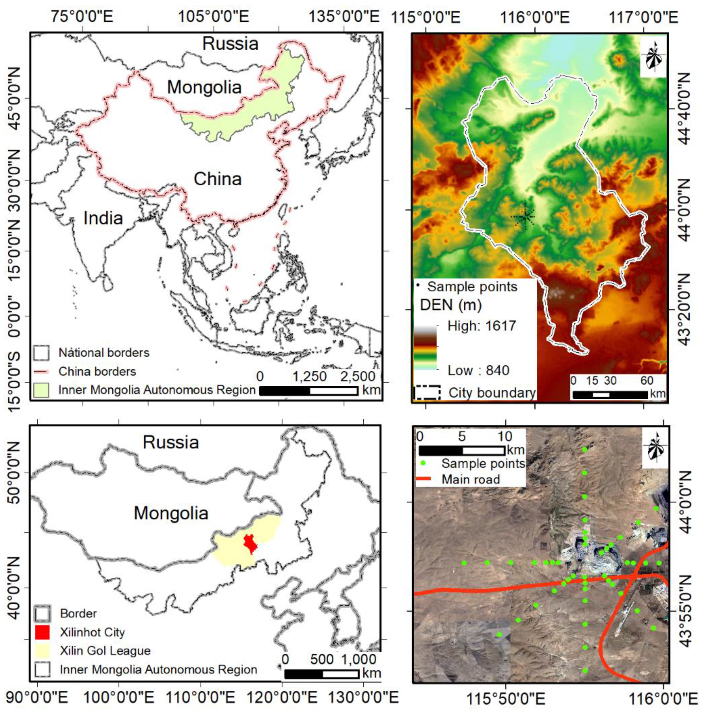
2.1. Study Area

The West No. 1 open-pit mine and the West No. 2 open-pit mine of Shengli coalfield in the Xilinguole area, Inner Mongolia, were selected as the research. The Shengli coalfield of Xilinguole League is in the Xilinguole area of Inner Mongolia and is about 4 km from the western boundary of Xilinhot City, whose jurisdiction it is under. The climate of the study area is temperate and semi-arid grassland. The weather during winter is mostly cold and dry, and the summer is mainly warm and humid. From the months of March to May each year, there is often strong wind, and the monthly average wind speed can reach 4.9 m/s. The average annual precipitation is 33.69 cm, and about 70% of rain occurs from May to August each year. The frost-free period from April to October lasts for about 150 days. The annual evaporation is about 160–180 cm, which is 4 or 5 times higher than the annual precipitation (Figure 1).

2.2. Sample Design and Data Acquisition

Mining area location data (shape file data, Figure 1) were collected from Inner Mongolia Agricultural University, which has been serving the mining sector in Inner Mongolia. The data were strictly validated based on Google Earth image and field data. The accuracy of validation reached 95%. Using the Google Earth remote sensing image of the map and the method of labor measurement [20], the boundaries of the West No. 1 open-pit mine and the West No. 2 open-pit mine were determined, and the range within 8 km of the mining boundary was taken as the research area. The mining area was taken as the center and a radius was created around in to form the survey sample lines. According to the remote sensing results and the actual situation of the mining area, a survey sample line with a length of 4 km was set in the east direction of the mining area. Since there is a large-scale wind power plant in the northwest of the mining area, and in order to avoid affecting the accuracy and validity of the experimental data, no survey sample line was set in the northwest of the mining area. At the same time, ArcGIS 10.0 was used to extract random sample points near the high-grade highway in the study area, and DEM data were extracted according to the points; terrain slope data and distance data from the highway were also generated.
Taking the mining area as the middle line, one research sample line was set in seven directions, namely east, south, west, north, southeast, southwest, and northeast; in combination with the actual situation around the mining area, a total of five survey sample sites were set on the sample line in the east direction at 0 km, 0.5 km, 1 km, 2 km, and 4 km from the outer boundary of the mining area. In the remaining six sample belt directions, seven survey sample lands were set at 0 km, 0.5 km, 1 km, 2 km, 4 km, 6 km, and 8 km from the outer boundary of the mining area (Figure 1). A GPS location system was used to record the basic geographic information of each sampling site in detail.
The soil collection time lasted from July to the end of September in 2018. Within the sample area, an area of 100 × 100 m2 was selected in advance for preliminary sampling. Then, a 100 m sample line diagonally crossing the selected area was chosen, with six survey sample plots, numbered C1–C6, set on the sample line, whose area was 1 × 1 m2. In the odd sample plots, surface soil samples were collected using a soil drill with a diameter of 5 cm, and the general collection depth was 0–10 cm. The drilling frequency of each sample was set at 5 times. The obtained samples were mixed evenly and collected with plastic bags and then marked and brought back to the laboratory. After natural drying in the laboratory, sand and gravel remains were removed as well as those of plants and other impurities by sifting them through a 100-mesh sieve for proper preservation in preparation for the subsequent analysis.
On the premise of fully studying the content of heavy metals in coal mine rocks, six kinds of heavy metal elements that can clearly reflect the indexes, namely Cr, Cu, Mn, Ni, Zn, and Pb, were selected as the objects for this measurement. The total amount was measured using the open decocting method with the solvent of chlorozotocin acid–perchloric acid (HNO3-HCl-HClO4), and the heavy metal content was measured by ICP-OES [21].
The NDVI dataset consists of atmospherically corrected surface reflectance data from the Landsat 8 OLI/TIRS sensors. These images contain 5 visible and near-infrared (VNIR) bands and 2 short-wave infrared (SWIR) bands processed to orthorectified surface reflectance, and two thermal infrared (TIR) bands processed to orthorectified brightness temperature. This product was supplied by USGS (USGS https://www.usgs.gov/, accessed on 1 May 2021). The spatial resolution of the dataset was 30 m, and the data acquisition time was from 2013 to 2018. Finally, the arithmetic average of images with less than 40% cloud coverage from June to September in summer was calculated. The infrared band corresponded to B5 (0.851–0.879 μm) of Landsat 8, and the red band corresponded to B4 (0.636–0.673 μm) [22].
N D V I = B 5 B 4 B 5 + B 4

2.3. Methods

2.3.1. Spatial Data Generation and Data Processing

The slope was extracted from SRTM (Shuttle Radar Topography Mission V4.1), and the generated DEM data were resampled to 250 m resolution. The NDVI dataset is based on continuous time series SPOT/VEGETATION NDVI satellite remote sensing data and is generated using the maximum value synthesis method. In the process of measuring the content of heavy metals in soil, the SPSS 16.0 single sample K–S test method was used to test the normal distribution of the data; the data of various heavy metals were fitted with the help of ArcGIS Desktop 10.5 software, and then, a spatial distribution map was generated as an output.

2.3.2. Maximum Difference Method

The maximum value comparison method takes the difference between the maximum value and the background value of the soil heavy metal element I in the study area as the research object to screen out the types of soil heavy metals whose maximum value exceeds the background value (also known as the safety warning value) and the distribution of this type. This method only evaluates whether the heavy metal content exceeds the standard and the spatial distribution range of pollution, and the results are intuitive and readable.
Δ H = M a x C i B i
where C i is the measured content of the soil heavy metal element i (mg/kg) and B i is the regional background value of the soil heavy metal element i (mg/kg). In the spatial distribution of heavy metals, the background value may not be an integer, and the decimal is truncated to take the integer upward. The calculation of the background value is based on the average content of heavy metals in the soil in the north, south, and west of the mining area, 10 km away from the mine, which better reflects the pollution of the surrounding soil due to open-pit coal mining.

2.3.3. Coefficient of Variation

The coefficient of variation is a standardized measurement method of probability distribution or frequency distribution. When the coefficient of variation is low, the data have less variability and higher stability. The spatial variability of soil and vegetation characteristics can be expressed by C V .
C V = S x ¯ × 100 %
where C V is the coefficient of variation, s is the standard deviation, and x ¯ is the average value. It is generally believed that C V < 10% denotes weak variability, 10% ≤ C V ≤ 100% denotes medium variability, and C V > 100% denotes strong variability.

2.3.4. Semivariogram

In the early 1960s, the French geologist G. Matheron [23] proposed the semivariogram, which is used to describe the spatial characteristics of the coexistence of structural and stochastic characteristics of regionalized variables [24,25] and to express the spatial variability and correlation degree of regionalized variables on a certain scale. Assuming that the mean value of the random function is stable, variance exists and is limited and the value is only related to the interval h , the semivariogram function γ ¯ ( h ) can be defined as half of the incremental variance of the random function Z ( x ) . A semivariogram has an independent variable and a dependent variable like ordinary functions. The independent variable is step h , and the dependent variable is a semivariogram value γ ¯ ( h ) .
γ ¯ ( h ) = 1 2 N ( h ) i = 1 N ( h ) [ Z ( x i ) Z ( x i + h ) ] 2
where x is the sample point, x i is the attribute value of sample point i , and N ( h ) is the logarithm of points with distance h . Therefore, the value of the semivariogram is the average value of the square of the difference between the sample point x and the attribute of the sample point h .
A semivariogram is usually characterized by three parameters [26]: (1) nugget variance (Co), which is mainly caused by spatial variation and measurement error; (2) structural variance (Co + C), which generally represents the maximum variance between data pairs; and (3) range (A), which represents the farthest distance of correlation between graphic parameters. The experimental variogram is a discontinuous distribution function obtained from the collected data, which need to be fitted by the theoretical variogram to obtain a continuous evaluation of variability [27].
In the process of studying the spatial differentiation of geographical objects or phenomena, the most important parameter of a variogram is the ratio of nugget value to abutment value. The ratio represents the proportion of spatial heterogeneity caused by human activities in the total variation of the system, while the base value represents the role of the composition of the natural environment. The lower the ratio is, the more significantly it is affected by the natural environment. The higher the ratio is, the greater the impact of human activities is. If the ratio is lower than 25%, it indicates that the system has a strong spatial correlation, which is mainly caused by the structural effect of the natural environment. If the ratio is between 25% and 75%, it indicates that the system has a medium spatial correlation, which indicates that its spatial change is the result of the joint action of the natural environment factors and the random factors of human activities. If the ratio is higher than 75%, the spatial correlation of the system is very weak, and the variation is more significantly affected by human activities.

2.3.5. Spatial Local Interpolation of Heavy Metals in Soil Surface

Kriging interpolation, also known as spatial local interpolation, is a method of unbiased optimal estimation of regionalized variables in a limited area based on variogram theory and structural analysis [28]. To use the kriging interpolation method for prediction, the first step is to create a variogram. Through semivariogram modeling, the spatial autocorrelation of spatial samples is analyzed. Then, the unknown value is predicted by the semivariogram estimation model.
Z * ( x 0 ) = i = 1 n λ i Z ( x i )
where Z * ( x 0 ) is the estimated value of the electricity to be measured, Z ( x i ) is the measured value of the i-th sample point, n is the number of measured samples participating in the calculation, and λ i is the weight coefficient of the i-th sample point. The weight is obtained by unbiased estimation and minimum variance of kriging interpolation. The calculation is as follows:
{ i = 1 n γ ¯ ( x i x j ) λ i + μ = γ ¯ ( x 0 x j )   ( j = 1 , 2 , , n ) i = 1 n λ i = 1
where γ ¯ ( x i x j ) is the semivariogram between the i-th and j-th sample points and γ ¯ ( x 0 x j ) is the semivariogram between the j-th sample point and the interpolation point, both of which can be obtained from the fitted variogram; μ is the Lagrange multiplier and n is the number of sample points.

2.3.6. Linear Regression Test

Suppose that a dependent variable y is affected by k independent variables x 1 , x 2 , …, x k . The n groups of observations are ( y a , x 1 a , x 2 a , …, x k a ), a = 1 , 2 , , n . Then, the structure of the multiple linear regression model is as follows:
y a = β 0 + β 1 x 1 a + β 2 x 2 a + + β k x k a + ε a
where β 0 , β 1 , , β k are the undetermined parameters and ε a is a random variable.

3. Results

3.1. Basic Characteristics of Heavy Metal Content in Surface Soil of Mining Area

According to descriptive statistics (Table 1), there is no abnormal value in the data. A normality test was carried out for Cr, Cu, Mn, Ni, Zn, and Pb. As the sample size of the research data was more than 50, the Kolmogorov–Smirnov test (K–S test) was used [29]. According to the p-value of the K–S test, Zn and Pb showed significant differences (p < 0.05), but they did not have normal characteristics. Cr, Cu, Mn, and Ni did not show significant differences (p > 0.05), but they were normal. At the same time, according to the C V value, it was found that Zn has weak variability while the other heavy metal elements have medium variability, which indicates that the heavy metals in the soil of the mining area are greatly affected by the external environment and human activities.

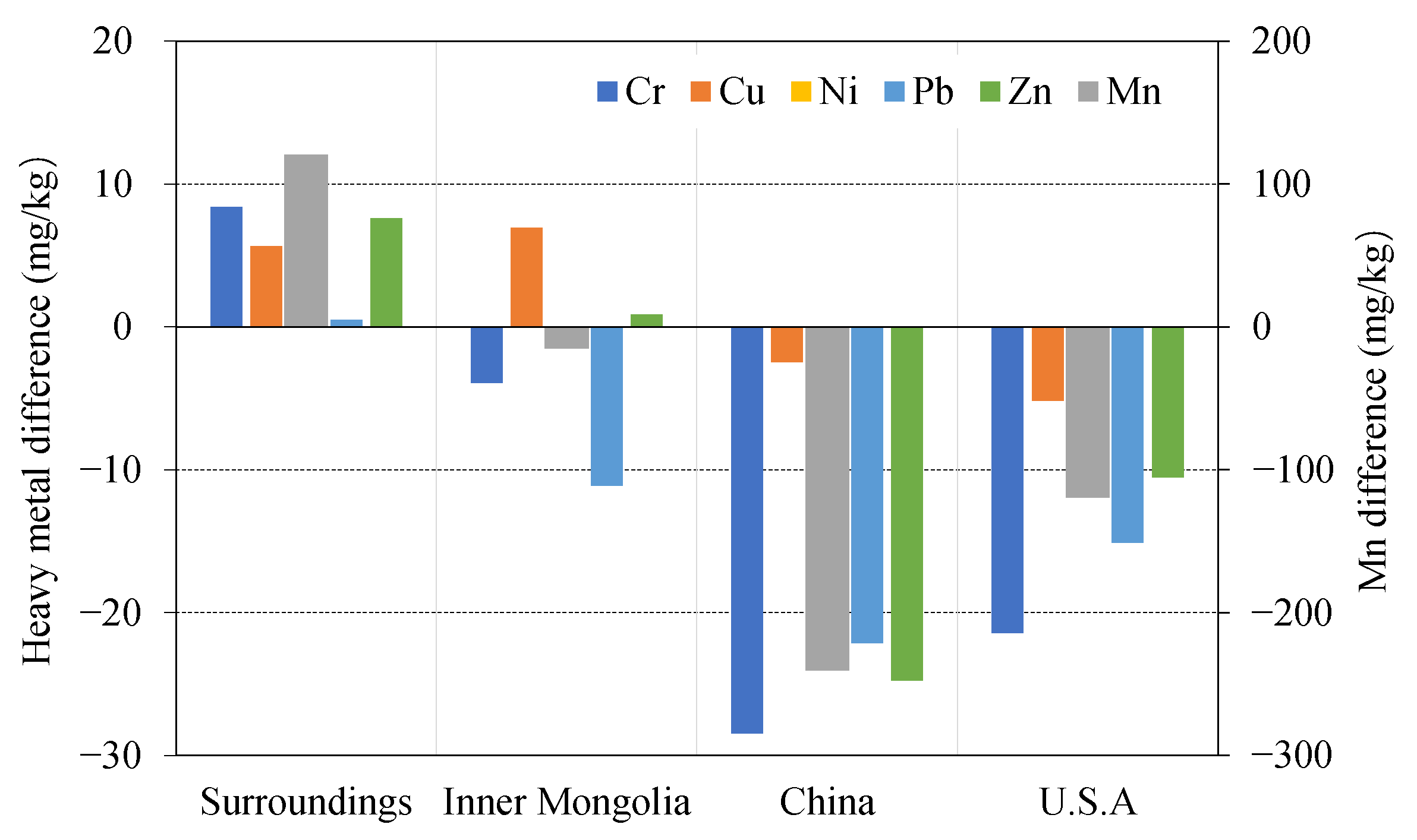
3.2. Difference between the Maximum and Background Values of Heavy Metals in Surface Soil of Mining Area

In previous studies, different criteria were selected as reference values according to research needs [30,31]. The purpose of this study was to evaluate whether the heavy metal concentrations in the surface soil around the mining area exceed the standard caused by open-pit coal mining and to compare the element background values in the study area to those in other areas. The average values of soil heavy metal contents (surroundings) and the background values of soil (layer A) in Inner Mongolia, China, and the United States in the northern, southern, and western directions of the mining area were selected as the reference values to compare and analyze the changes in heavy metal contents in the surface soil of the mining area. It was found that the contents of heavy metals in the surface soil of the mining area are higher than those of surrounding areas; Cu and Zn are higher than the background values of Inner Mongolia, but all values are lower than the national background values, indicating that the mining area and nearby soil are significantly affected by coal mining (Figure 2).

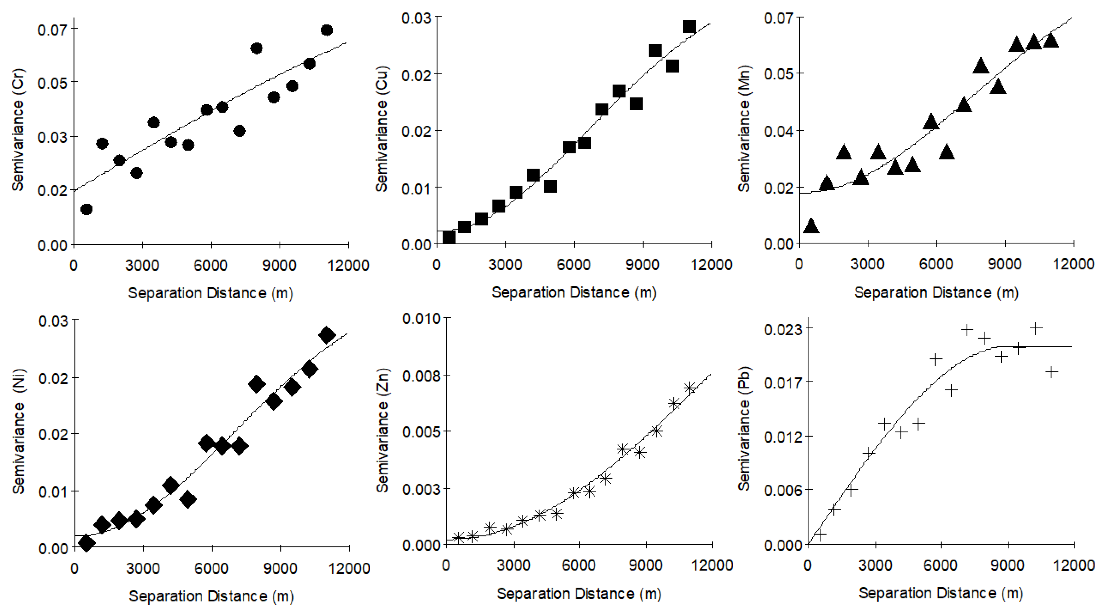
3.3. Semivariogram Analysis of Heavy Metals in Soil of Coal Mining Area

In order to avoid the scale effect, deform the variogram, raise the nugget variance and structural sill, increase the estimation error, and cover up the inherent structure, GS + 9.0 was used for logarithmic transformation of Zn and Pb, which do not conform to normal characteristics. The transformed data met the assumptions of geostatistical analysis. The semivariogram model was used to fit the graph and the determination coefficient was comprehensively considered. According to the principle that R2 is the largest, RSS is the smallest, and the range is greater than the sample spacing, the optimal semivariogram function model (Figure 3) was selected and the relevant parameters were obtained (Table 2). The results showed that Cu, Mn, Ni, and Zn conform to a Gaussian model, while Cr and Pb conform to a spherical model. The fitting degree of the six heavy metals’ data and the semivariogram function model was good, reaching 0.792–0.986. Therefore, to meet the relevant statistical requirements (Table 2), the semivariogram model could be used, and the accuracy also meets the requirements of spatial difference.
The ratio of nugget value to abutment value is an important indicator to reflect the degree of spatial heterogeneity of regionalized variables [32], which reflects the dominant role of structural factors (natural factors) or random factors (human factors) in the composition of spatial variation. This study found that Cr, Cu, Mn, Ni, Zn, and Pb are the most important elements in the regional variation. The ratio of nugget value to abutment value of the six heavy metal elements was more than 75% (Table 2), which indicates that the spatial distribution of the six elements in soil is mainly caused by human activities rather than natural distribution or evolution.

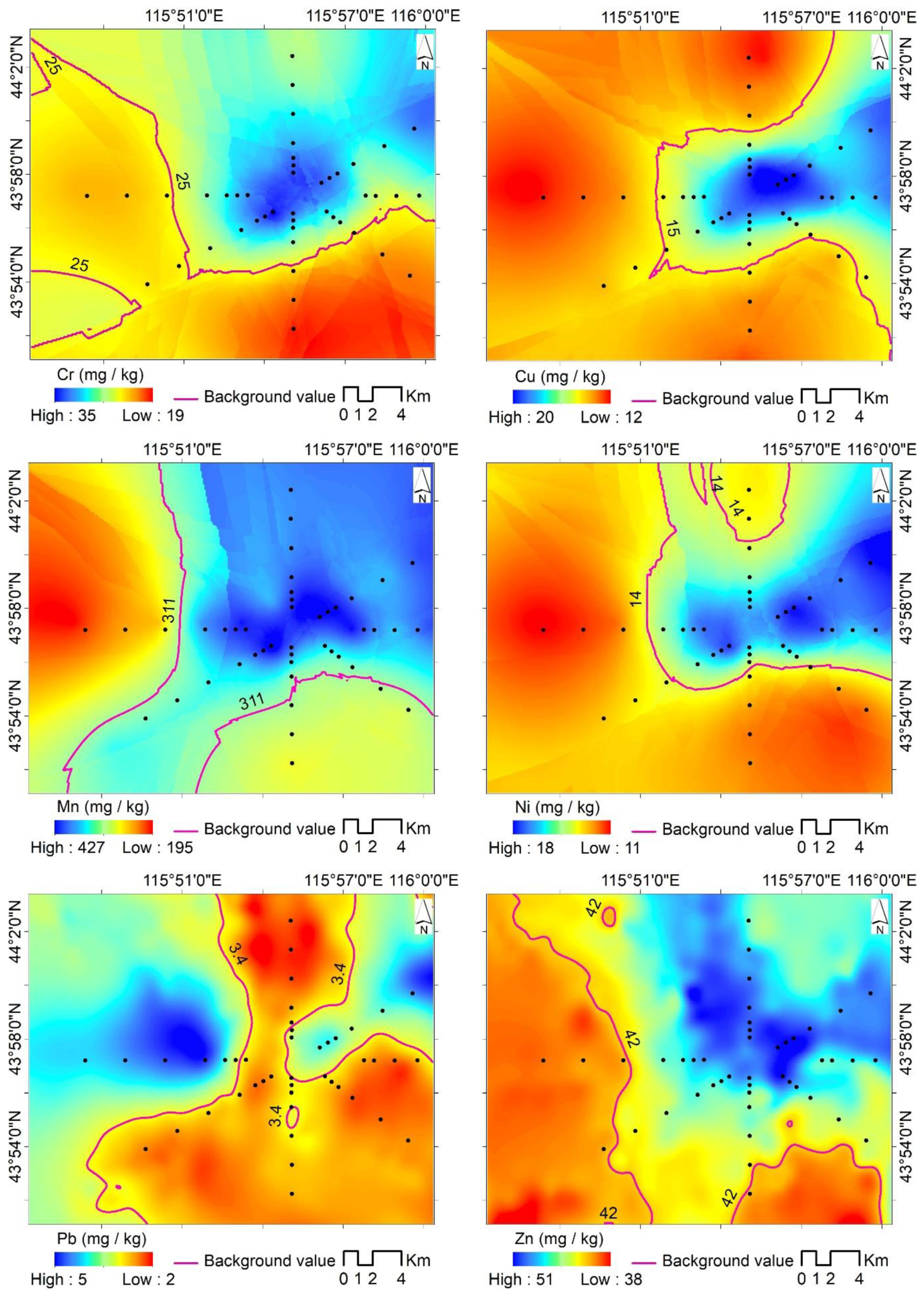
3.4. Spatial Distribution Characteristics of Soil Heavy Metal Content

Due to the spatial differentiation of heavy metal enrichment in soil in some regions and the lack of statistical data in some regions, it is difficult to accurately reflect the actual situation of soil by simply using sample data for analysis and evaluation [32]. The kriging model essentially estimates the value of variables in regions without data by using the original data of regionalized variables and the structural characteristics of a variogram. Combined with the previous research on the spatial distribution characteristics of soil heavy metals, based on the selection standard of the heavy metal interpolation method [33], an error comparison of the surface soil interpolation method (Table 3) was obtained. The results showed that the optimal interpolation method of Cr, Cu, Mn, and Ni in the mining area is ordinary kriging, and the optimal interpolation method of Zn is simple kriging.
Spatial differentiation is a process to simulate and generate the real spatial distribution characteristics of elements using spatial modeling [34]. Based on the parameters of the semivariogram model (Table 2) and kriging type (Table 3), the spatial differences of six heavy metals in the soil near the mining area were analyzed using ArcGIS 10.5 (Figure 4).
It can be seen from Figure 2 that the Cr content was the highest in the soil in the center of the mining area, and the Cr content in the center, north, and northeast of the mining area was significantly higher than that in the other directions, showing a flaky spreading distribution. The area where the heavy metal content exceeded the background value of the surrounding environment accounted for 46.24% of the study area; the content of Cu and Ni was centered in the mining area, showing a “core” distribution slightly higher than that in the other directions extending to the east and northeast, and these elements exceeded the background value by 29.49% and 33.08%, respectively. The distribution of Mn and Zn showed a diffuse distribution from northeast to southwest, exceeding the background value by 53.71% and 65.10%, respectively, and the part exceeding the background value divided the study area into two parts. The difference was that the distribution of Mn exceeding the background value was more concentrated in the northeast of the study area, while the distribution of Pb was convex to the southwest; in total, 52.17% of the study area had a Pb content over the background value. The spatial distribution of Pb in the surface soil showed a “dual core” distribution.

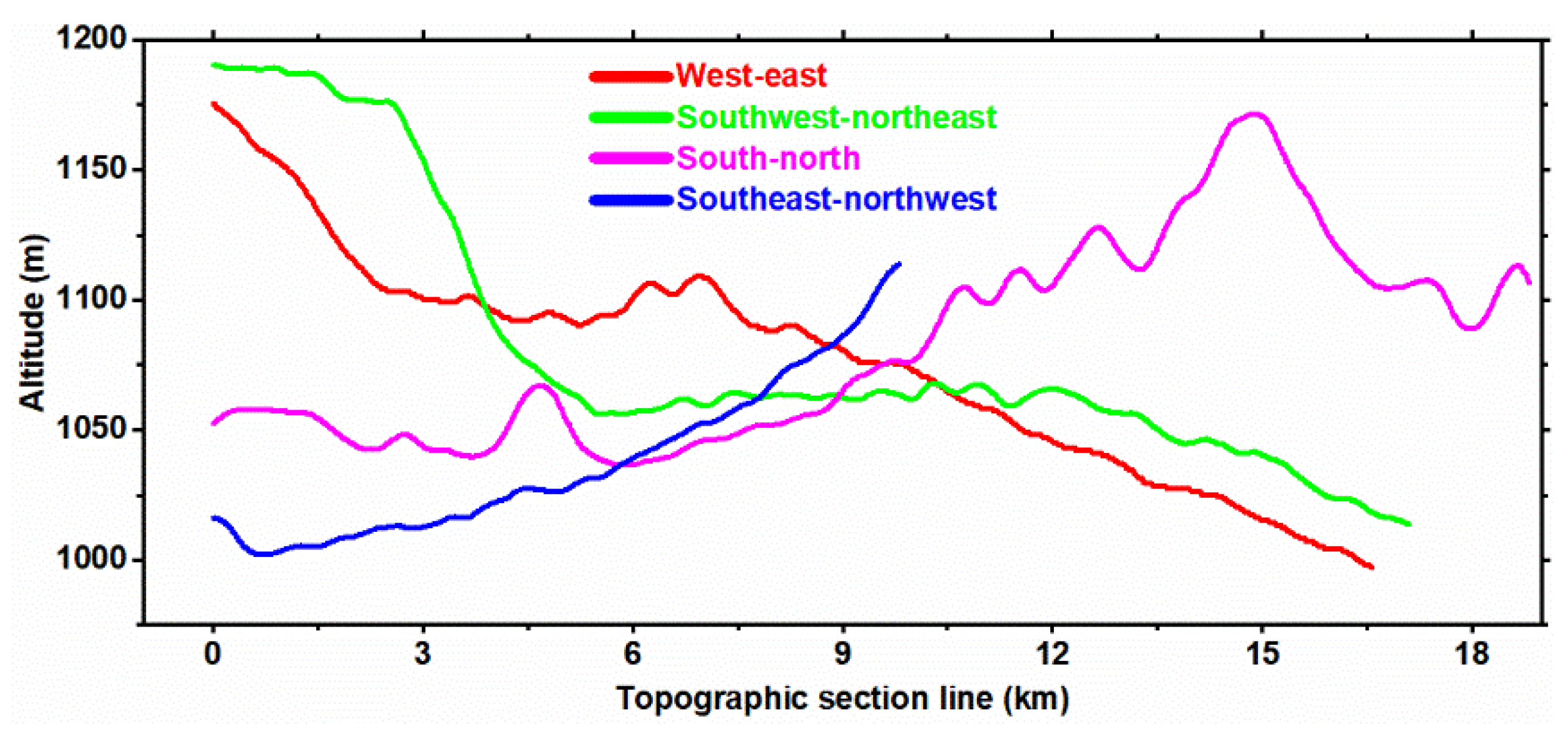
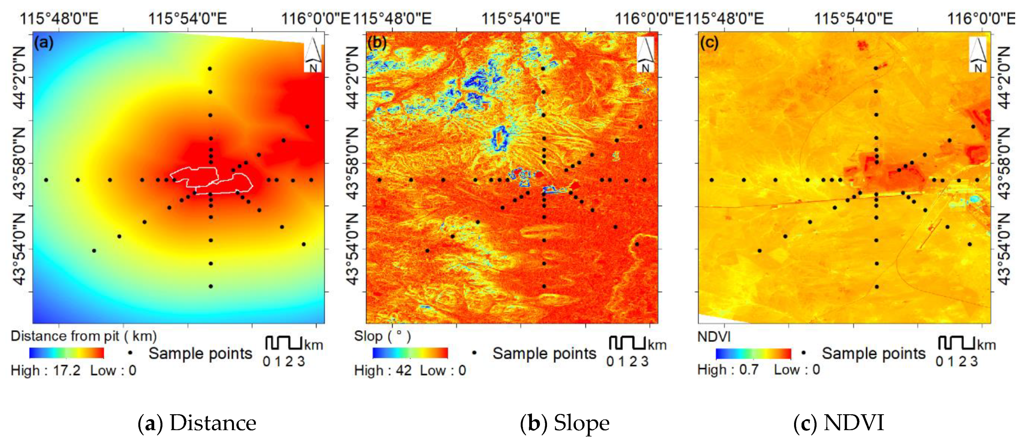
3.5. Analysis of Factors Influencing the Spatial Distribution of Heavy Metals

In order to further quantitatively analyze the spatial distribution pattern [33] of heavy metals in the mining area, a stepwise regression model was established with six heavy metal elements as dependent variables and distance from the pit, slope (Figure 5, a profile that can reflect the change of slope at different points in different directions), and NDVI as independent variables (Figure 6a–c, and Table 4). The R-squared and adjusted R-squared values of all heavy metals except Pb were close to 1, indicating that the fitting degree was high, and there was a negative correlation with the mine distance; Cr, Mn, and Zn had a positive correlation with slope, while Cu had a negative correlation. Ni and Pb had no obvious correlation with slope and NDVI had a negative correlation with Cu and Ni but no significant correlation with Cr, Mn, or Pb. The F-value of Cr, Cu, Mn, Ni, and Zn was greater than 3.40, and the p-value was less than 0.01, which indicates that all heavy metal elements except Pb had a significant linear correlation with distance, slope, and NDVI.

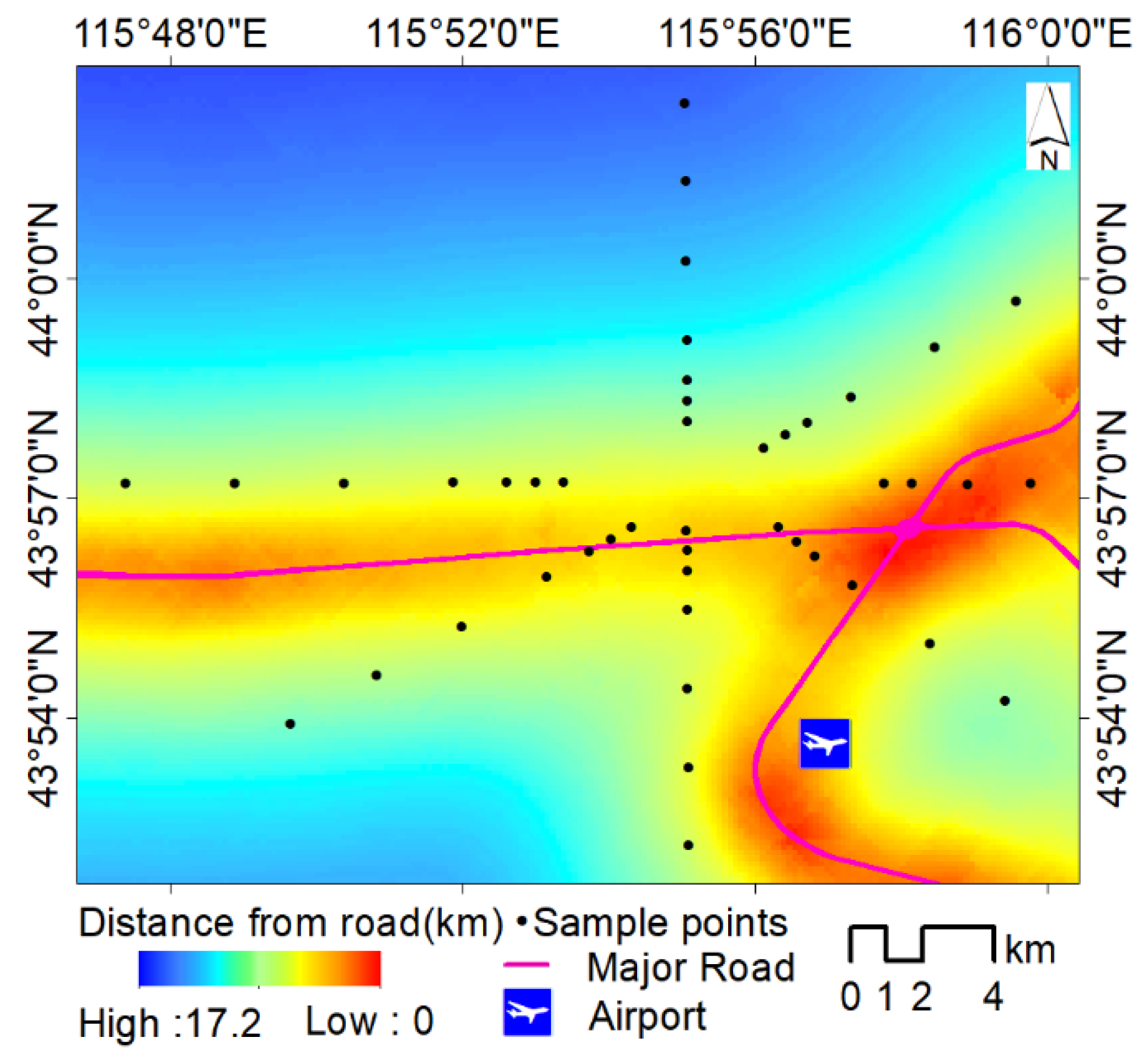
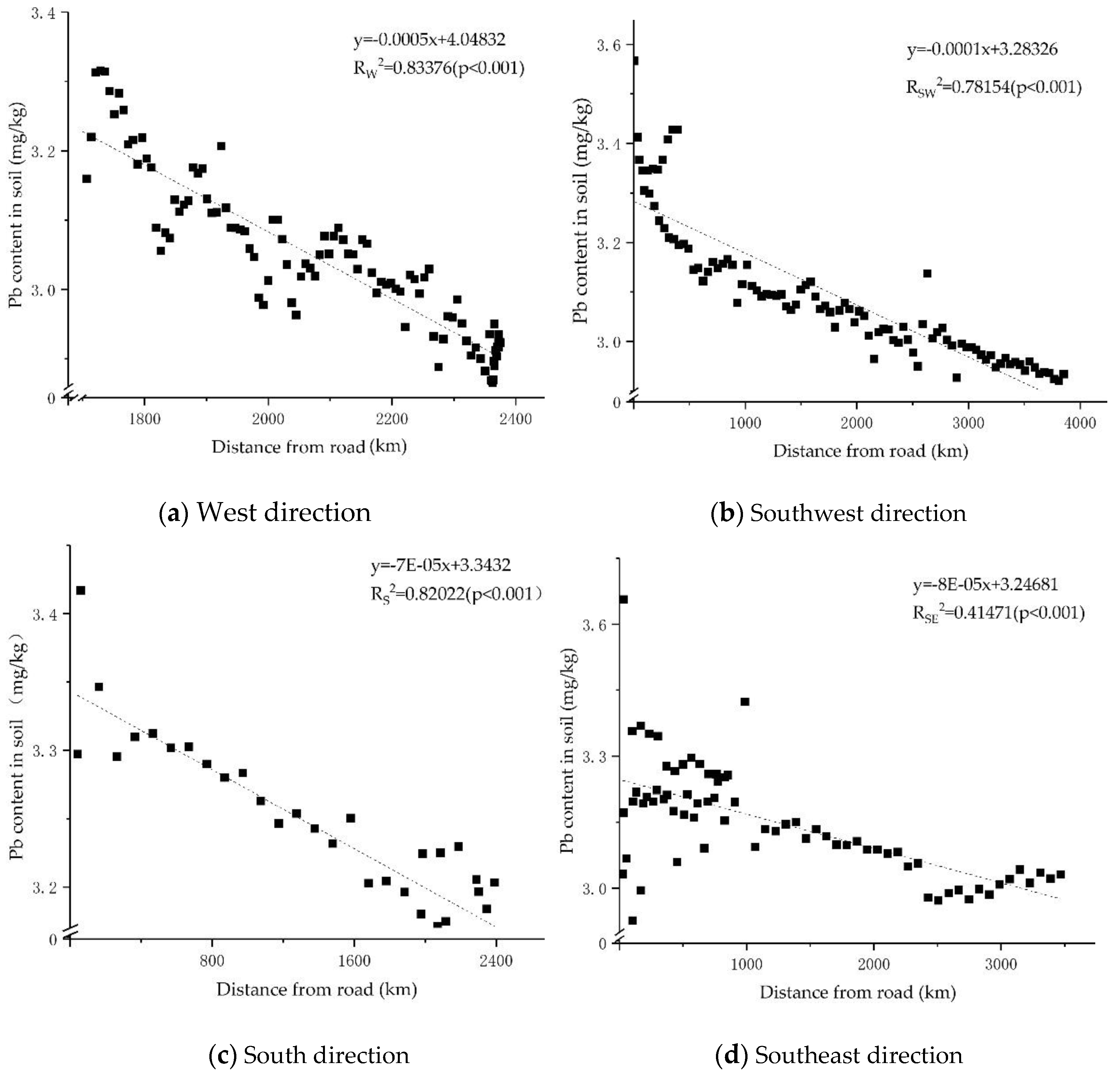
3.6. Analysis of Influencing Factor of Pb

The relationship between Pb in soil and mining distance, slope, and NDVI was not obvious. Based on the characteristics of surface mining production, the relationship between the lead content around the mining area and road transportation was analyzed. The lead content may be affected by road transportation (Figure 7). Using ArcGIS 10.5, random points were generated in various line directions, and a regression function was established according to the distance between each point’s lead content and the road around the mining area [35]. It was found that lead content in the west, southwest, south, and southeast of the mining area was positively related to road distance. The correlation between the Pb content and road distance follows the order of RW2 > RSW2 > RS2 > RES2 (Figure 8), and the longest road does not exceed 4 km. In the true west direction of the sample point, the impact of the road was very significant, while the north and northeast contain mostly village roads, which are not suitable for coal transportation, so the relationship between lead content and roads was not significant.

4. Discussion

From the perspective of research methods, the introduction of statistical methods into the study of soil properties and spatial–temporal distribution can not only improve the efficiency and level of information processing and analysis but also serve as a supplement to the traditional research methods of the spatial variability of soil properties [4,36]. Therefore, the spatial distribution characteristics of heavy metals can be quantitatively described by statistical methods. In general, the heavy metal pollution in the mining area has the distribution characteristics of point, line, ring, and band, showing a spatial distribution pattern of pollution in the upper, surface, and underground areas. The content of heavy metals in the soil was the highest in the center of the mining area, being slightly higher in the east, north, and northeast than in other directions, and was inversely proportional to the distance from the mining area. The data show that the local open-pit coal mining has a certain impact on the soil around the mining area and increases the content of heavy metals in the soil. However, soil heavy metals have obvious temporal variability. In this study, only the relevant factors of spatial variability were analyzed. In the future research, the temporal and spatial differentiation of heavy metals should be discussed further. As the spatiotemporal Kruger method is suitable for the analysis of location, time, and multi-attribute motion data [37], it can realize the assimilation of multi-source spatiotemporal datasets [38], such as those from tracking research of animals, plants, and spatiotemporal phenomena in different historical periods [39,40].
From the perspective of influencing factors, the effect of diffusion factors on soil cannot be ignored. The distribution of heavy metals is affected by the prevailing wind direction [41], pollutant deposition, vegetation coverage, landform, rivers, and human activities. This diffusion will lead to a great change in the content of heavy metals in the soil in different directions. As there is no river around the mining area, heavy metal pollutants mainly appear from atmospheric deposition and particle diffusion. Except for southeasterly wind in summer, the other seasons in the mining area mainly experience southwesterly wind. Therefore, as the mining area is in the downwind direction [3], the content of heavy metals in the north and northeast is significantly higher than in other directions.
Additionally, the density of human activities also has a significant impact on the enrichment of heavy metals in soil. For example, the sampling point in the east of the mining area is not only affected by the dominant wind direction but also by the urban area. At the same time, the open-pit mining in the study area resulted in the accumulation pattern of heavy metal elements in the soil that diffused from the central area of the coal mine to the surrounding area [19,42]. Heavy metal emissions from heavy machinery and truck transportation are also potential environmental risks, forming a strip pattern of pollution [43]. For example, in the west and south of the mining area (W, SW, S, SE), the sample point’s Pb value was significantly affected by road transportation, while the topography and vegetation had a significant influence on Cr, Cu, Mn, Ni, and Zn but not on Pb. All of these can be used to draw a high-precision distribution of heavy metal pollution in the soil by interpolation method [5,44].
In conclusion, in the process of industrialization and urbanization, mining industry and urban activities are very important factors affecting the spatial distribution of heavy metals in soil [45]. In particular, it is necessary to fully understand the content and distribution of heavy metals in the soil in a timely manner and strengthen environmental protection measures within the scope of human activities so as to prevent heavy metal pollution and ensure the healthy and sustainable development of the mining area [11,46].

5. Conclusions

The content of heavy metals in the surface soil of the study area was higher than the background value of heavy metals in the grassland around the mining area, but lower than the background value of Inner Mongolia. According to the structure effect and random effect of the semivariogram, the content of heavy metals in the mining area and its surrounding surface soil is mainly affected by external human activities and is not formed naturally. Among the heavy metal pollution, Cr, Cu, and Ni form the pollution within the mining area, while Mn, Zn, and Pb form the diffusion pollution. The other five heavy metal elements, except Pb, are affected by distance, slope, and NDVI. The high-grade highway has a significant impact on the lead content in the surface soil of the mining area. In view of the heavy metal deposition in the grassland mining area, it is necessary to prevent secondary pollution caused by transportation of large amount of coal resources. In this paper, the source, spatial distribution, and diffusion characteristics of heavy metal pollutants in the coal mining area are discussed. These can provide reference cases for the study of heavy metals in other mining areas and provide a scientific basis for the decision-making of environmental governance in the coal mining area.

Author Contributions

Investigation, Xinyao Liu; supervision, Mingjiu Wang; writing—original draft, Guoqing Chen; writing—review and editing, Yong Yang. All authors have read and agreed to the published version of the manuscript.

Funding

This work was funded by the Inner Mongolia Science and Technology Agency (Grant No. 2020ZD0020-3).

Acknowledgments

We thank the reviewers and Petr Jeremic for their valuable comments.

Conflicts of Interest

The authors declare no conflict of interest.

References

  1. Gruszecka-Kosowska, A. Human Health Risk Assessment and Potentially Harmful Element Contents in the Fruits Cultivated in the Southern Poland. Int. J. Environ. Res. Public Health 2019, 16, 5096. [Google Scholar] [CrossRef] [Green Version]
  2. Nyssen, J.; Jacob, M.; Frankl, A. Part V Geomorphic Processes/Sediment Yield and Reservoir Siltation in Tigray. In Geo-Trekking in Ethiopia’s Tropical Mountains; Springer Nature Switzerland AG: Cham, Switzerland, 2019. [Google Scholar]
  3. Othmani, M.A.; Souissi, F.; Duraes, N.; Abdelkader, M.; da Silva, E.F. Assessment of metal pollution in a former mining area in the NW Tunisia: Spatial distribution and fraction of Cd, Pb and Zn in soil. Environ. Monit. Assess. 2015, 187, 523. [Google Scholar] [CrossRef] [PubMed]
  4. Santos-Frances, F.; Martinez-Grana, A.; Zarza, C.A.; Sanchez, A.G.; Rojo, P.A. Spatial Distribution of Heavy Metals and the Environmental Quality of Soil in the Northern Plateau of Spain by Geostatistical Methods. Int. J. Environ. Res. Public Health 2017, 14, 568. [Google Scholar] [CrossRef] [PubMed]
  5. Park, J.; Kwon, E.; Chung, E.; Kim, H.; Battogtokh, B.; Woo, N.C. Environmental Sustainability of Open-Pit Coal Mining Practices at Baganuur, Mongolia. Sustainability 2019, 12, 248. [Google Scholar] [CrossRef] [Green Version]
  6. Trifuoggi, M.; Pagano, G.; Oral, R.; Gravina, M.; Toscanesi, M.; Mozzillo, M.; Siciliano, A.; Burić, P.; Lyons, D.M.; Palumbo, A. Topsoil and urban dust pollution and toxicity in Taranto (southern Italy) industrial area and in a residential district. Environ. Monit. Assess. 2018, 191, 43. [Google Scholar] [CrossRef]
  7. Gonzalez-Fernandez, B.; Rodriguez-Valdes, E.; Boente, C.; Menendez-Casares, E.; Fernandez-Brana, A.; Gallego, J.R. Long-term ongoing impact of arsenic contamination on the environmental compartments of a former mining-metallurgy area. Sci. Total Environ. 2018, 610–611, 820–830. [Google Scholar] [CrossRef] [PubMed]
  8. Muyessar, T.; Jilili, A.; Jiang, F.-Q. Distribution characteristics of soil heavy metal content in northern slope of Tianshan Mountains and its source explanation. Chin. J. Eco-Agric. 2013, 21, 883–890. [Google Scholar] [CrossRef]
  9. Bityukova, L. Heavy metals in the soils of Tallinn (Estonia) and its suburbs. Geomicrobiol. J. 1993, 11, 285–298. [Google Scholar] [CrossRef]
  10. Deckers, S.; Tielens, S.; Geyndt, K.D.; Wauw, J.V.d.; Nyssen, J. Part I Setting the Scene/24 Understanding soil spatial patterns for sustainable development. In Geo-Trekking in Ethiopia’s Tropical Mountains; Springer Nature Switzerland AG: Cham, Switzerland, 2019. [Google Scholar]
  11. Dolezalova Weissmannova, H.; Mihocova, S.; Chovanec, P.; Pavlovsky, J. Potential Ecological Risk and Human Health Risk Assessment of Heavy Metal Pollution in Industrial Affected Soils by Coal Mining and Metallurgy in Ostrava, Czech Republic. Int. J. Environ. Res. Public Health 2019, 16, 4495. [Google Scholar] [CrossRef] [PubMed] [Green Version]
  12. Gabarrón, M.; Faz, A.; Acosta, J.A. Effect of different industrial activities on heavy metal concentrations and chemical distribution in topsoil and road dust. Environ. Earth Sci. 2017, 76. [Google Scholar] [CrossRef]
  13. Jian, G.L.; Mason, P.J.; Yu, E.; Wu, M.C.; Tang, C.; Huang, R.; Liu, H. GIS modelling of earthquake damage zones using satellite remote sensing and DEM data. Geomorphology 2012, 139, 518–535. [Google Scholar]
  14. Boluwade, A. Joint Simulation of Spatially Correlated Soil Health Indicators, Using Independent Component Analysis and Minimum/Maximum Autocorrelation Factors. ISPRS Int. J. Geo-Inf. 2020, 9, 30. [Google Scholar] [CrossRef] [Green Version]
  15. Aerzuna, A.; Wang, J.; Wang, H.; Rukeye, S.; Abdugheni, A.; Umut, H. Spatial distribution analysis of heavy metals in soil and atmospheric dust fall and their relationships in Xinjiang Eastern Junggar mining area. Trans. Chin. Soc. Agric. Eng. 2017, 33, 259–266. [Google Scholar]
  16. Santos-Frances, F.; Martinez-Grana, A.; Alonso Rojo, P.; Garcia Sanchez, A. Geochemical Background and Baseline Values Determination and Spatial Distribution of Heavy Metal Pollution in Soils of the Andes Mountain Range (Cajamarca-Huancavelica, Peru). Int. J. Environ. Res. Public Health 2017, 14, 859. [Google Scholar] [CrossRef] [PubMed] [Green Version]
  17. Tezel, D.; Inam, S.; Kocaman, S. GIS-Based Assessment of Habitat Networks for Conservation Planning in Kas-Kekova Protected Area (Turkey). ISPRS Int. J. Geo-Inf. 2020, 9, 91. [Google Scholar] [CrossRef] [Green Version]
  18. Plyatsuk, L.; Balintova, M.; Chernysh, Y.; Demcak, S.; Holub, M.; Yakhnenko, E. Influence of Phosphogypsum Dump on the Soil Ecosystem in the Sumy region (Ukraine). Appl. Sci. 2019, 9, 5559. [Google Scholar] [CrossRef] [Green Version]
  19. Zwolak, A.; Sarzyńska, M.; Szpyrka, E.; Stawarczyk, K. Sources of Soil Pollution by Heavy Metals and Their Accumulation in Vegetables: A Review. Water Air Soil Pollut. 2019, 230. [Google Scholar] [CrossRef] [Green Version]
  20. Wang, W.; Shen, R.P.; Cao-Xiang, J.I. Study on Heavy Metal Cu based on Hyperspectral Remote Sensing. Remote Sens. Technol. Appl. 2011, 26, 348–354. [Google Scholar]
  21. Edokpayi, J.; Odiyo, J.; Popoola, O.; Msagati, T. Assessment of Trace Metals Contamination of Surface Water and Sediment: A Case Study of Mvudi River, South Africa. Sustainability 2016, 8, 135. [Google Scholar] [CrossRef] [Green Version]
  22. Gozdowski, D.; Stpień, M.; Panek, E.; Varghese, J.; Samborski, S. Comparison of winter wheat NDVI data derived from Landsat 8 and active optical sensor at field scale. Remote Sens. Appl. Soc. Environ. 2020, 20. [Google Scholar] [CrossRef]
  23. Matheron, G. Principle of Geostatistics. Econ. Geol. 1963, 58, 1246–1266. [Google Scholar] [CrossRef]
  24. Setiyoko, A.; Basaruddin, T.; Arymurthy, A.M. Minimax Approach for Semivariogram Fitting in Ordinary Kriging. IEEE Access 2020, 8, 82054–82065. [Google Scholar] [CrossRef]
  25. Moonchai, S.; Chutsagulprom, N. Semiparametric Semivariogram Modeling with a Scaling Criterion for Node Spacing: A Case Study of Solar Radiation Distribution in Thailand. Mathematics 2020, 8, 2173. [Google Scholar] [CrossRef]
  26. Eze, P.N.; Kumahor, S.K. Gaussian process simulation of soil Zn micronutrient spatial heterogeneity and uncertainty–A performance appraisal of three semivariogram models. Sci. Afr. 2019, 5, e00110. [Google Scholar] [CrossRef]
  27. Zhang, H.; Wang, X.S. The impact of groundwater depth on the spatial variance of vegetation index in the Ordos Plateau, China: A semivariogram analysis. J. Hydrol. 2020, 588, 125096. [Google Scholar] [CrossRef]
  28. Mirás-Avalos, J.M.; Fandiño, M.; Rey, B.J.; Dafonte, J.; Cancela, J.J. Zoning of a Newly-Planted Vineyard: Spatial Variability of Physico-Chemical Soil Properties. Soil Syst. 2020, 4, 62. [Google Scholar] [CrossRef]
  29. Liu, X.; Zhang, Y.; Li, P. Spatial Variation Characteristics of Soil Erodibility in the Yingwugou Watershed of the Middle Dan River, China. Int. J. Environ. Res. Public Health 2020, 17, 3568. [Google Scholar] [CrossRef]
  30. Colak, M. Heavy metal concentrations in sultana-cultivation soils and sultana raisins from Manisa (Turkey). Environ. Earth Sci. 2012, 67, 695–712. [Google Scholar] [CrossRef]
  31. Ahmad, N.; Hussain, J.; Ahmad, I.; Asif, M. Estimation of health risk to humans from heavy metals in soil of coal mines in Harnai, Balochistan. Int. J. Environ. Anal. Chem. 2020, 1–12. [Google Scholar] [CrossRef]
  32. Mahboob, M.A.; Celik, T.; Genc, B. Predictive modeling and comparative evaluation of geostatistical models for geochemical exploration through stream sediments. Arab. J. Geosci. 2020, 13, 1080. [Google Scholar] [CrossRef]
  33. Grynyshyna-Poliuga, O. Characteristic of modelling spatial processes using geostatistical analysis. Adv. Space Res. 2019, 64, 415–426. [Google Scholar] [CrossRef]
  34. Tenreiro, T.R.; García-Vila, M.; Gómez, J.A.; Jimenez-Berni, J.A.; Fereres, E. Water modelling approaches and opportunities to simulate spatial water variations at crop field level. Agric. Water Manag. 2020, 240, 106254. [Google Scholar] [CrossRef]
  35. Bei, Z.; Yong, Y. Spatiotemporal modeling and prediction of soil heavy metals based on spatiotemporal cokriging. Sci. Rep. 2017, 7. [Google Scholar] [CrossRef]
  36. Mohammad, Z.M.; Ruhollah, T.M.; Ali, A. Evaluation of Geostatistical Techniques for Mapping Spatial Distribution of Soil PH, Salinity and Plant Cover Affected by Environmental Factors in Southern Iran. Not. Sci. Biol. 2010, 2, 92–103. [Google Scholar]
  37. Li, Q.; Pei, J.; Zhang, J.; Han, B. SUM: Suboptimal Unitary Multi-Task Learning Framework for Spatiotemporal Data Prediction. In Proceedings of the CIKM 2019—28th ACM International Conference on Information and Knowledge Management, Beijing, China, 3–7 November 2019. [Google Scholar]
  38. Yang, B.; Liu, H.; Kang, E.L.; Shu, S.; Yu, B. Spatio-temporal Cokriging method for assimilating and downscaling multi-scale remote sensing data. Remote Sens. Environ. 2020, 255. [Google Scholar] [CrossRef]
  39. Rojo, J.; Pérez-Badia, R. Spatiotemporal analysis of olive flowering using geostatistical techniques. Sci. Total Environ. 2015, 505, 860–869. [Google Scholar] [CrossRef] [PubMed]
  40. Lamb, D.S.; Downs, J.; Reader, S. Space-Time Hierarchical Clustering for Identifying Clusters in Spatiotemporal Point Data. ISPRS Int. J. Geo-Inf. 2020, 9, 85. [Google Scholar] [CrossRef] [Green Version]
  41. Zaborska, A.; Beszczynska-Moller, A.; Wlodarska-Kowalczuk, M. History of heavy metal accumulation in the Svalbard area: Distribution, origin and transport pathways. Environ. Pollut. 2017, 231, 437–450. [Google Scholar] [CrossRef]
  42. Guan, Z.; Li, X.; Wang, L. Heavy metal enrichment in roadside soils in the eastern Tibetan Plateau. Environ. Sci. Pollut. Res. 2018, 25, 7625–7637. [Google Scholar] [CrossRef]
  43. Karan, S.K.; Samadder, S.R. Reduction of spatial distribution of risk factors for transportation of contaminants released by coal mining activities. J. Environ. Manag. 2016, 180, 280–290. [Google Scholar] [CrossRef]
  44. Schwarz, A.; Wilcke, W.; Kobža, J.; Zech, W. Spatial distribution of soil heavy metal concentrations as indicator of pollution sources at Mount Križna (Great Fatra, central Slovakia). J. Plant Nutr. Soil Sci. 1999, 162, 421–428. [Google Scholar] [CrossRef]
  45. Zeng, S.; Ma, J.; Ren, Y.; Liu, G.J.; Zhang, Q.; Chen, F. Assessing the Spatial Distribution of Soil PAHs and their Relationship with Anthropogenic Activities at a National Scale. Int. J. Environ. Res. Public Health 2019, 16, 4928. [Google Scholar] [CrossRef] [PubMed] [Green Version]
  46. Song, D.; Jiang, D.; Wang, Y.; Chen, W.; Huang, Y.; Zhuang, D. Study on association between spatial distribution of metal mines and disease mortality: A case study in Suxian District, South China. Int. J. Environ. Res. Public Health 2013, 10, 5163–5177. [Google Scholar] [CrossRef] [PubMed]
Figure 1. Location of the research area and distribution of the sampling sites.
Ijgi 10 00290 g001
Figure 2. Statistical analysis of heavy metals in soil of mining area.
Ijgi 10 00290 g002
Figure 3. Parameters of the semivariogram model for heavy metal content in surface soil of coal mining area.
Ijgi 10 00290 g003
Figure 4. Kriging interpolation prediction chart of soil heavy metal content.
Ijgi 10 00290 g004
Figure 5. Topographic profile of the study area along the sampling line.
Ijgi 10 00290 g005
Figure 6. Distance (a), slope (b), and NDVI (c) from the mine in the study area.
Ijgi 10 00290 g006
Figure 7. Distance map between sample points and main roads in the study area.
Ijgi 10 00290 g007
Figure 8. Regression diagram of Pb content in the soil of the mining area and distance from highway. (ad) are significant at the p < 0.001 level.
Ijgi 10 00290 g008
Table 1. The statistical features of concentrations of heavy metals in soil of mining area.
Heavy MetalsMinimum
(mg/kg)
Maximum
(mg/kg)
Mean ± SD
(mg/kg)
SkewnessKurtosisK–S TestCoefficient of Variation ( C V )Background Value of Reference Area
SurroundingsInner MongoliaChinaU.S.A
D p(mg/kg)(mg/kg)(mg/kg)(mg/kg)
Cr18.5144.4927.538 ± 5.8400.620.2220.0680.7821.21%9.724.1836.561
Cu12.7219.716.228 ± 2.023−0.148−1.2170.1070.1412.47%10.214.2112.922.3
Mn174.87505.97352.562 ± 70.469−0.3410.3840.0780.58419.99%9.34310.27446583
Ni11.6317.6214.854 ± 1.790−0.225−1.310.1050.15612.05%10.6913.1717.326.9
Zn40.2749.9545.764 ± 2.702−0.579−0.7270.1330.020 *5.91%22.4941.8948.674.2
Pb2.764.643.411 ± 0.4700.9420.0560.1650.001 **13.79%16.963.391526
Table 2. The types of soil heavy metals.
Heavy MetalsNugget VarianceStructural SillRangeProportionR2ResidualModel
CoCo + CAC/(Co + C)RSSVariogram Model Type
Cr1.71 × 10−20.084 22,870 0.797 0.792 0.001 Spherical
Cu1.60 × 10−30.036 9370 0.955 0.973 0.000 Gaussian
Mn1.56 × 10−20.091 10,570 0.828 0.890 0.001 Gaussian
Ni1.40 × 10−30.036 9810 0.961 0.960 0.000 Gaussian
Zn2.10 × 10−40.020 17,810 0.990 0.986 0.000 Gaussian
Pb1.00 × 10−50.021 9090 1.000 0.938 0.000 Spherical
Table 3. Error comparison of spatial interpolation methods for heavy metal content in surface soil of mining area.
Heavy MetalsKriging TypeMean StandardizedRoot Mean SquareAverage Mean ErrorRoot Mean Square Standardized
CrOrdinary−0.0033.4223.4950.939
Simple0.0183.9843.7500.862
Universal−0.0023.8014.4320.733
Indicator−0.0023.4303.4690.929
Probability0.0104.4354.4890.864
Disjunctive0.0084.1964.2850.871
CuOrdinary−0.0020.4640.5280.907
Simple−0.0310.5160.6630.796
Universal−0.3890.5310.0500.842
Indicator0.0060.7750.3620.775
Probability−0.0090.5640.5870.833
Disjunctive−0.0310.5160.6630.796
MnOrdinary−0.00947.32047.2080.917
Simple−0.00849.03551.1200.909
Universal−0.21447.32042.1440.693
Indicator−0.03949.35748.4151.016
Probability−0.10248.35846.4101.200
Disjunctive−0.00849.03551.1200.989
NiOrdinary−0.0390.4470.4330.857
Simple−0.0380.4650.6300.782
Universal−0.7990.4470.4050.430
Indicator0.0090.4790.4940.759
Probability0.0490.4980.3990.754
Disjunctive−0.0380.4830.5300.782
ZnOrdinary0.1340.8840.8390.569
Simple−0.0060.8600.8711.005
Universal−0.1190.8840.8210.730
Indicator0.0050.9800.8730.804
Probability0.0070.8760.9790.787
Disjunctive0.1341.0101.7190.569
PbOrdinary0.0250.3260.2430.503
Simple0.0190.2550.3560.622
Universal−0.0060.3090.3580.887
Indicator0.0540.3490.3930.529
Probability0.0630.3360.3890.745
Disjunctive0.0130.2720.3740.674
Table 4. Linear regression results of heavy metal elements in surface soil of mining area with pit distance and NDVI (n = 44).
Heavy
Metals
FactorUnstandardized CoefficientsStandardized CoefficientstpVIFR2Adjusted
R2
F
BStd. ErrorBeta
CrConstant31.24 1.23 -25.38 0.000 **-0.770.753F (3,40) = 44.726, p = 0.000
Distance0.00 0.00 −0.89 −10.71 0.000 **1.21
Slope0.46 0.16 0.23 2.87 0.007 **1.14
NDVI−11.15 9.18 −0.10 −1.21 0.231.09
CuConstant20.36 0.54 -37.84 0.000 **-0.8440.832F (3,40) = 71.961, p = 0.000
Distance0.00 0.00 −0.70 −10.20 0.000 **1.21
Slope−0.25 0.07 −0.24 −3.60 0.001 **1.14
NDVI−18.56 4.01 −0.30 −4.62 0.000 **1.09
MnConstant411.05 18.41 -22.33 0.000 **-0.7230.702F (3,40) = 34.720, p = 0.000
Distance−0.02 0.00 −0.83 −9.06 0.000 **1.21
Slope6.50 2.40 0.24 2.71 0.010 **1.14
NDVI−274.74 137.36 −0.17 −2.00 0.05 1.09
NiConstant17.17 0.56 -30.78 0.000 **-0.7830.767F (3,40) = 48.085, p = 0.000
Distance0.00 0.00 −0.83 −10.28 0.000 **1.21
Slope−0.01 0.07 −0.01 −0.06 0.951.14
NDVI−8.43 4.16 −0.16 −2.02 0.050 *1.09
PbConstant3.61 0.32 -11.27 0.000 **-0.021−0.053F (3,40) = 0.281, p = 0.839
Distance0.00 0.00 −0.08 −0.45 0.651.21
Slope−0.01 0.04 −0.02 −0.13 0.901.14
NDVI−1.44 2.39 −0.10 −0.60 0.551.09
ZnConstant48.43 0.76 -63.50 0.000 **-0.8190.806F (3,40) = 60.462, p = 0.000
Distance0.00 0.00 −0.91 −12.32 0.000 **1.21
Slope0.36 0.10 0.26 3.59 0.001 **1.14
NDVI−10.14 5.69 −0.13 −1.78 0.081.09
The symbol * indicates the statistical significance at the 0.05 level, and the symbol ** indicates the statistical significance at the 0.01 level.
Publisher’s Note: MDPI stays neutral with regard to jurisdictional claims in published maps and institutional affiliations.

