
Assessing Influential Factors on Inland Property Damage from Gulf of Mexico Tropical Cyclones in the United States


Abstract
:1. Introduction
2. Materials and Methods
2.1. Study Area
2.2. Data
2.2.1. TC-Related Property Damage
2.2.2. Influential Factors
- TC tracks.
- TC rainfall.
- TC wind.
- County social vulnerability.
- Elevation.
- Other data.
2.3. Data Analyses
3. Results
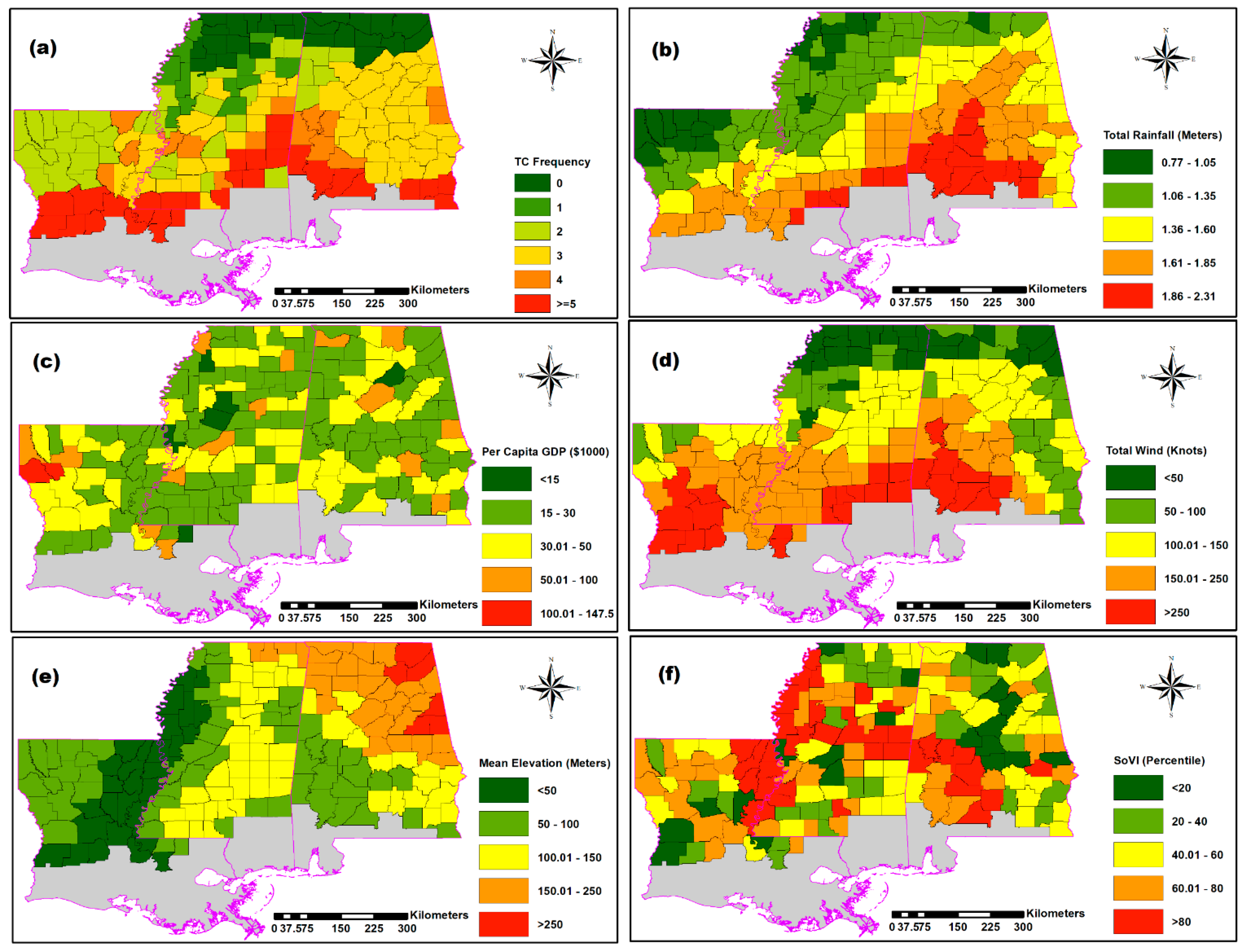
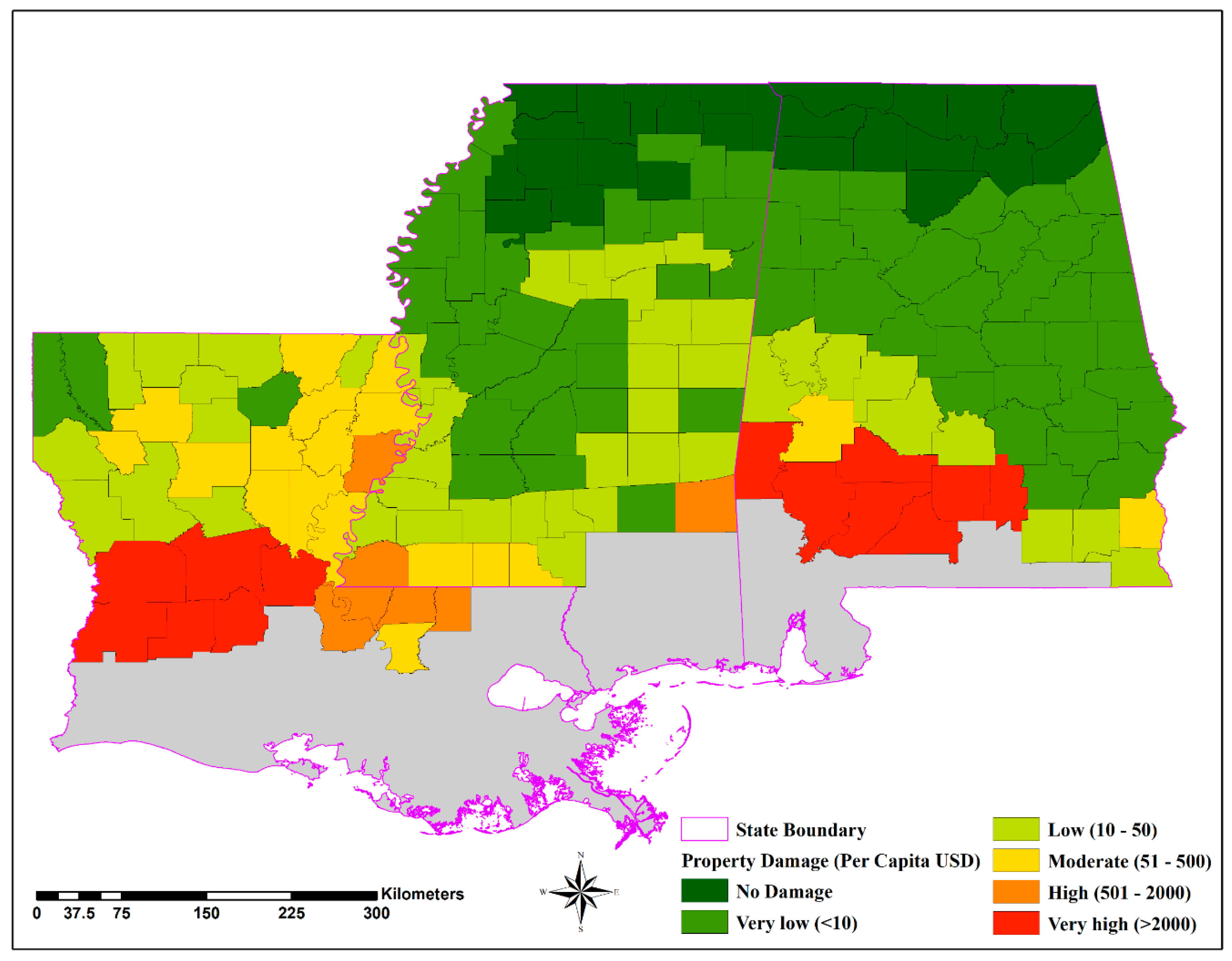
3.1. Spatial Patterns of Property Damage and Influential Factors
3.2. Influential Factors on Property Damage
3.2.1. OLS Results
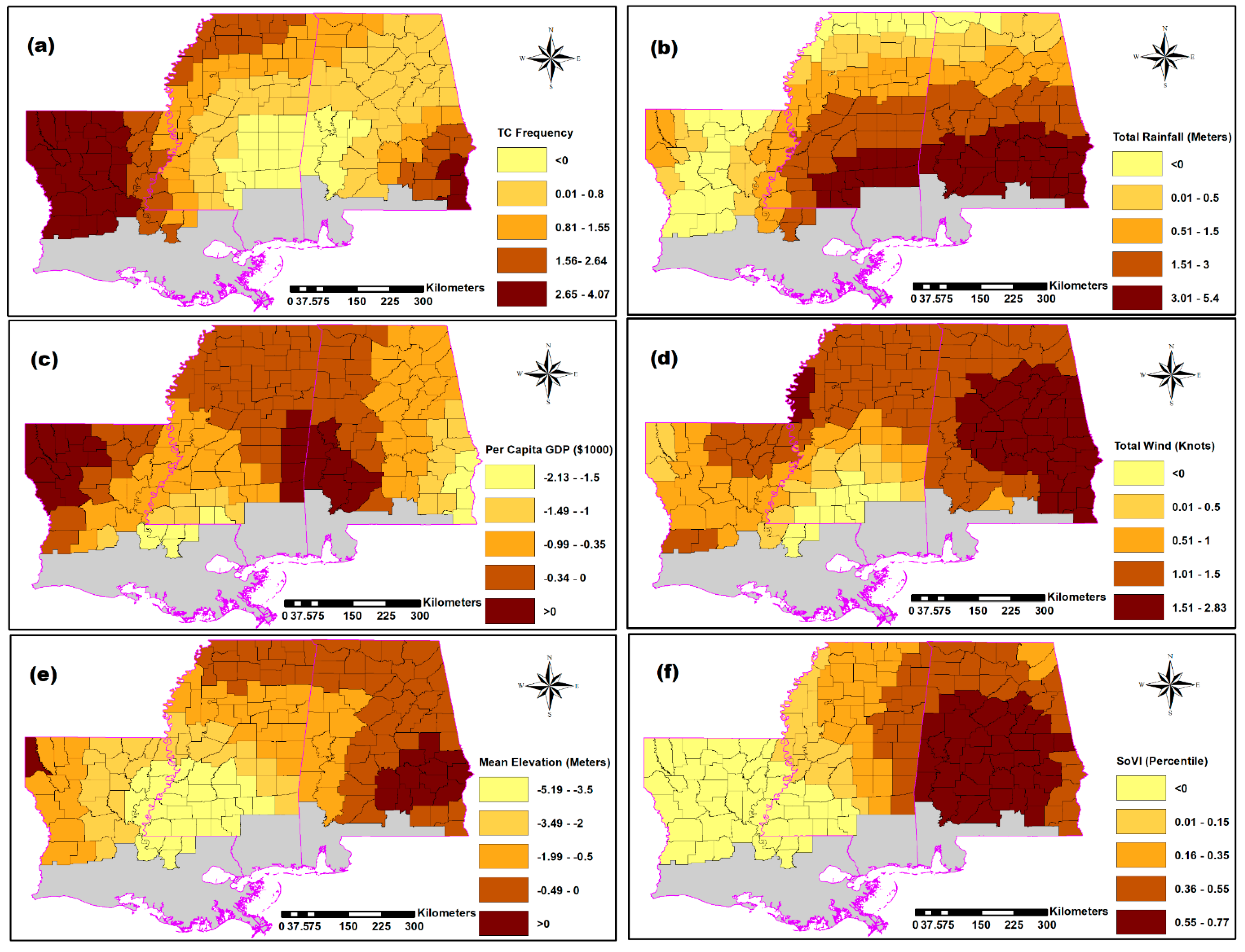
3.2.2. GWR Results
3.2.3. OLS and GWR Model Comparison
4. Discussion
5. Conclusions
Author Contributions
Funding
Institutional Review Board Statement
Informed Consent Statement
Data Availability Statement
Acknowledgments
Conflicts of Interest
References
- Peduzzi, P.; Chatenoux, B.; Dao, H.; De Bono, A.; Herold, C.; Kossin, J.; Mouton, F.; Nordbeck, O. Global trends in tropical cyclone risk. Nat. Clim. Chang. 2012, 2, 289–294. [Google Scholar] [CrossRef]
- Bakkensen, L.A.; Mendelsohn, R.O. Risk and adaptation: Evidence from global hurricane damages and fatalities. J. Assoc. Environ. Resour. Econ. 2016, 3, 555–587. [Google Scholar] [CrossRef] [Green Version]
- Bakkensen, L.A.; Shi, X.; Zurita, B.D. The impact of disaster data on estimating damage determinants and climate costs. Econ. Disasters Clim. Chang. 2018, 2, 49–71. [Google Scholar] [CrossRef]
- Narita, D.; Tol, R.S.J.; Anthoff, D. Damage costs of climate change through intensification of tropical cyclone activities: An application of FUND. Clim. Res. 2009, 39, 87–97. [Google Scholar] [CrossRef]
- Ranson, M.; Kousky, C.; Ruth, M.; Jantarasami, L.; Crimmins, A.; Tarquinio, L. Tropical and extratropical cyclone damages under climate change. Clim. Chang. 2014, 127, 227–241. [Google Scholar] [CrossRef] [Green Version]
- Arndt, D.S.; Basara, J.B.; McPherson, R.A.; Illston, B.G.; McManus, G.D.; Demko, D.B. Observations of the overland reintensification of Tropical Storm Erin. Bull. Am. Meteorol. Soc. 2009, 90, 1079–1094. [Google Scholar] [CrossRef]
- Chang, H.; Niyogi, D.; Kumar, A.; Kishtawal, C.M.; Dudhia, J.; Chen, F.; Mohanty, U.C.; Shepherd, M. Possible relation between land surface feedback and the post-landfall structure of monsoon depressions. Geophys. Res. Lett. 2009, 36. [Google Scholar] [CrossRef]
- Lian-Shou, C. Research progress on the structure and intensity change for the landfalling tropical cyclones. J. Trop. Meteorol. 2012, 18, 113. [Google Scholar]
- Emanuel, K.; Callaghan, J.; Otto, P. A hypothesis for the redevelopment of warm-core cyclones over northern Australia. Mon. Weather Rev. 2008, 136, 3863–3872. [Google Scholar] [CrossRef]
- Ye, M.; Wu, J.; Liu, W.; He, X.; Wang, C. Dependence of tropical cyclone damage on maximum wind speed and socioeconomic factors. Environ. Res. Lett. 2020, 15. [Google Scholar] [CrossRef]
- Pielke, R.A., Jr. Future economic damage from tropical cyclones: Sensitivities to societal and climate changes. Philos. Trans. R. Soc. A Math. Phys. Eng. Sci. 2007, 365, 2717–2729. [Google Scholar] [CrossRef] [PubMed]
- Pielke, R.A., Jr.; Gratz, J.; Landsea, C.W.; Collins, D.; Saunders, M.A.; Musulin, R. Normalized hurricane damage in the United States: 1900–2005. Nat. Hazards Rev. 2008, 9, 29–42. [Google Scholar] [CrossRef]
- Burton, C.G. Social vulnerability and hurricane impact modeling. Nat. Hazards Rev. 2010, 11, 58–68. [Google Scholar] [CrossRef]
- Senkbeil, J.C.; Brommer, D.M.; Comstock, I.J. Tropical cyclone hazards in the USA. Geogr. Compass 2011, 5, 544–563. [Google Scholar] [CrossRef]
- Mendelsohn, R.; Emanuel, K.; Chonabayashi, S.; Bakkensen, L. The impact of climate change on global tropical cyclone damage. Nat. Clim. Chang. 2012, 2, 205–209. [Google Scholar] [CrossRef]
- Weinkle, J.; Landsea, C.; Collins, D.; Musulin, R.; Crompton, R.P.; Klotzbach, P.J.; Pielke, R. Normalized hurricane damage in the continental United States 1900–2017. Nat. Sustain. 2018, 1, 808–813. [Google Scholar] [CrossRef]
- Knabb, R.; Rhome, J.; Brown, D. National Hurricane Center. Tropical Cyclone Report: Hurricane Katrina, 23–30 August 2005. National Oceanic and Atmospheric Administration; National Weather Service, National Hurricane Center: Miami, FL, USA, 2005.
- Blake, E.S.; Landsea, C.; Gibney, E.J. The Deadliest, Costliest, and Most Intense United States Tropical Cyclones from 1851 to 2010 (and Other Frequently Requested Hurricane Facts); NOAA Technical Memorandum NWS NHC: Washington, DC, USA, 2011.
- Benfield, A. Weather, Climate and Catastrophe Insight: 2017 Annual Report; London Aon: London, UK, 2018; p. 56. [Google Scholar]
- Mestre, O.; Hallegatte, S. Predictors of tropical cyclone numbers and extreme hurricane intensities over the North Atlantic using generalized additive and linear models. J. Clim. 2009, 22, 633–648. [Google Scholar] [CrossRef]
- Anderson, W.F.; Maaß, A.; Ozias-Akins, P. Genetic Variability of a Forage Bermudagrass Core Collection. Crop. Sci. 2009, 49, 1347–1358. [Google Scholar] [CrossRef] [Green Version]
- Zhou, X.; Liu, Z.; Yan, Q.; Zhang, X.; Yi, L.; Yang, W.; Xiang, R.; He, Y.; Hu, B.; Liu, Y.; et al. Enhanced Tropical Cyclone Intensity in the Western North Pacific During Warm Periods Over the Last Two Millennia. Geophys. Res. Lett. 2019, 46, 9145–9153. [Google Scholar] [CrossRef]
- Senkbeil, J.C.; Sheridan, S.C. A postlandfall hurricane classification system for the United States. J. Coast. Res. 2006, 22, 1025–1034. [Google Scholar] [CrossRef]
- Kovach, M.M.; Konrad, C.E. The spatial distribution of tornadoes and high wind impacts associated with inland-moving tropical cyclones in the southeastern United States. Phys. Geogr. 2014, 35, 245–271. [Google Scholar] [CrossRef]
- Rappaport, E.N. Loss of life in the United States associated with recent Atlantic tropical cyclones. Bull. Am. Meteorol. Soc. 2000, 81, 2065–2074. [Google Scholar] [CrossRef] [Green Version]
- Cutter, S.L.; Mitchell, J.T.; Scott, M.S. Revealing the vulnerability of people and places: A case study of Georgetown County, South Carolina. Ann. Assoc. Am. Geogr. 2000, 90, 713–737. [Google Scholar] [CrossRef]
- Tierney, K.J.; Lindell, M.K.; Perry, R.W. Facing the Unexpected: Disaster Preparedness and Response in the United States; Joseph Henry Press: Washington, DC, USA, 2002. [Google Scholar]
- Cutter, S.L.; Boruff, B.J.; Shirley, W.L. Social vulnerability to environmental hazards. Soc. Sci. Q. 2003, 84, 242–261. [Google Scholar] [CrossRef]
- Emrich, C.T.; Cutter, S.L. Social vulnerability to climate-sensitive hazards in the Southern United States. Weather Clim. Soc. 2011, 3, 193–208. [Google Scholar] [CrossRef]
- Flanagan, B.E.; Gregory, E.W.; Hallisey, E.J.; Heitgerd, J.L.; Lewis, B. A social vulnerability index for disaster management. J. Homel. Secur. Emerg. Manag. 2011, 8. [Google Scholar] [CrossRef]
- Hossain, M.K.; Meng, Q. A thematic mapping method to assess and analyze potential urban hazards and risks caused by flooding. Comput. Environ. Urban. Syst. 2020, 79, 101417. [Google Scholar] [CrossRef]
- Hossain, M.K.; Meng, Q. A multi-decadal spatial analysis of demographic vulnerability to urban flood: A case study of Birmingham City, USA. Sustainability 2020, 12, 9139. [Google Scholar] [CrossRef]
- Ashley, W.S.; Strader, S.; Rosencrants, T.; Krmenec, A.J. Spatiotemporal changes in tornado hazard exposure: The case of the expanding bull’s-eye effect in Chicago, Illinois. Weather Clim. Soc. 2014, 6, 175–193. [Google Scholar] [CrossRef]
- Strader, S.M.; Ashley, W.S. The expanding bull’s-eye effect. Weatherwise 2015, 68, 23–29. [Google Scholar] [CrossRef]
- Freeman, A.C.; Ashley, W.S. Changes in the US hurricane disaster landscape: The relationship between risk and exposure. Nat. Hazards 2017, 88, 659–682. [Google Scholar] [CrossRef]
- Bierwagen, B.G.; Theobald, D.M.; Pyke, C.R.; Choate, A.; Groth, P.; Thomas, J.V.; Morefield, P. National housing and impervious surface scenarios for integrated climate impact assessments. Proc. Natl. Acad. Sci. USA 2010, 107, 20887–20892. [Google Scholar] [CrossRef] [PubMed] [Green Version]
- Rifat, S.A.A.; Liu, W. Quantifying Spatiotemporal Patterns and Major Explanatory Factors of Urban Expansion in Miami Metropolitan Area During 1992–2016. Remote Sens. 2019, 11, 2493. [Google Scholar] [CrossRef] [Green Version]
- Rijal, S.; Rimal, B.; Sloan, S. Flood hazard mapping of a rapidly urbanizing city in the foothills (Birendranagar, Surkhet) of Nepal. Land 2018, 7, 60. [Google Scholar] [CrossRef] [Green Version]
- Schmidt, S.; Kemfert, C.; Höppe, P. The impact of socio-economics and climate change on tropical cyclone losses in the USA. Reg. Environ. Chang. 2010, 10, 13–26. [Google Scholar] [CrossRef] [Green Version]
- Wen, S.; Wang, Y.; Su, B.; Gao, C.; Chen, X.; Jiang, T.; Tao, H.; Fischer, T.; Wang, G.; Zhai, J. Estimation of economic losses from tropical cyclones in China at 1.5 °C and 2.0 °C warming using the regional climate model COSMO-CLM. Int. J. Climatol. 2019, 39, 724–737. [Google Scholar] [CrossRef]
- Hallegatte, S. A normative exploration of the link between development, economic growth, and natural risk. Econ. Disasters Clim. Chang. 2017, 1, 5–31. [Google Scholar] [CrossRef] [Green Version]
- Wu, J.; Han, G.; Zhou, H.; Li, N. Economic development and declining vulnerability to climate-related disasters in China. Environ. Res. Lett. 2018, 13, 34013. [Google Scholar] [CrossRef]
- Wu, J.; Li, Y.; Li, N.; Shi, P. Development of an asset value map for disaster risk assessment in China by spatial disaggregation using ancillary remote sensing data. Risk Anal. 2018, 38, 17–30. [Google Scholar] [CrossRef]
- Czajkowski, J.; Kennedy, E. Fatal tradeoff? Toward a better understanding of the costs of not evacuating from a hurricane in landfall counties. Popul. Environ. 2010, 31, 121–149. [Google Scholar] [CrossRef]
- Czajkowski, J.; Simmons, K.; Sutter, D. An analysis of coastal and inland fatalities in landfalling US hurricanes. Nat. Hazards 2011, 59, 1513–1531. [Google Scholar] [CrossRef]
- Schmidlin, T.W. Human fatalities from wind-related tree failures in the United States, 1995–2007. Nat. Hazards 2009, 50, 13–25. [Google Scholar] [CrossRef]
- Powell, M.D.; Dodge, P.P.; Black, M.L. The landfall of Hurricane Hugo in the Carolinas: Surface wind distribution. Weather Forecast. 1991, 6, 379–399. [Google Scholar] [CrossRef]
- Senkbeil, J.C.; Myers, L.; Jasko, S.; Reed, J.R.; Mueller, R. Communication and hazard perception lessons from category five hurricane michael. Atmosphere 2020, 11, 804. [Google Scholar] [CrossRef]
- Kaplan, J.; DeMaria, M. A simple empirical model for predicting the decay of tropical cyclone winds after landfall. J. Appl. Meteorol. 1995, 34, 2499–2512. [Google Scholar] [CrossRef] [Green Version]
- Moore, T.W.; Dixon, R.W. Climatology of tornadoes associated with Gulf Coast-landfalling hurricanes. Geogr. Rev. 2011, 101, 371–395. [Google Scholar] [CrossRef]
- Rhodes, C.L.; Senkbeil, J.C. Factors contributing to tornadogenesis in landfalling Gulf of Mexico tropical cyclones. Meteorol. Appl. 2014, 21, 940–947. [Google Scholar] [CrossRef]
- Deo, A.A.; Ganer, D.W. Tropical cyclone activity over the Indian Ocean in the warmer climate. In Monitoring and Prediction of Tropical Cyclones in the Indian Ocean and Climate Change; Springer: Dordrecht, The Netherlands, 2014; pp. 72–80. [Google Scholar]
- Krishnamohan, K.S.; Mohanakumar, K.; Joseph, P. V Climate change in tropical cyclones and monsoon depressions of North Indian Ocean. In Monitoring and Prediction of Tropical Cyclones in the Indian Ocean and Climate Change; Springer: Dordrecht, The Netherlands, 2014; pp. 33–39. [Google Scholar]
- Yin, J.; Yin, Z.; Xu, S. Composite risk assessment of typhoon-induced disaster for China’s coastal area. Nat. Hazards 2013, 69, 1423–1434. [Google Scholar] [CrossRef]
- Cao, C.; Xu, P.; Wang, Y.; Chen, J.; Zheng, L.; Niu, C. Flash flood hazard susceptibility mapping using frequency ratio and statistical index methods in coalmine subsidence areas. Sustainability 2016, 8, 948. [Google Scholar] [CrossRef] [Green Version]
- Hossain, M.K.; Meng, Q. A fine-scale spatial analytics of the assessment and mapping of buildings and population at different risk levels of urban flood. Land Use Policy 2020, 99, 104829. [Google Scholar] [CrossRef]
- Rappaport, E.N.; Fernandez-Partagas, J. The Deadliest Atlantic Tropical Cyclones; National Hurricane Center: Washington, DC, USA, 1995; pp. 1492–1994.
- Blake, E.S.; Rappaport, E.N.; Landsea, C.W. The Deadliest, Costliest, and most Intense United States Tropical Cyclones from 1851 to 2006 (and Other Frequently Requested Hurricane Facts); NOAA/National Weather Service, National Centers for Environmental Prediction: Washington, DC, USA, 2007.
- Burroughs, W.J. Climate Change: A Multidisciplinary Approach; Cambridge University Press: Cambridge, UK, 2007; ISBN 1107049253. [Google Scholar]
- Camp, J.; Scaife, A.A.; Heming, J. Predictability of the 2017 North Atlantic hurricane season. Atmos. Sci. Lett. 2018, 19, 1–7. [Google Scholar] [CrossRef]
- Lavender, S.L.; Walsh, K.J.E.; Caron, L.P.; King, M.; Monkiewicz, S.; Guishard, M.; Zhang, Q.; Hunt, B. Estimation of the maximum annual number of North Atlantic tropical cyclones using climate models. Sci. Adv. 2018, 4, 1–8. [Google Scholar] [CrossRef] [Green Version]
- Doss, D.A.; Mcelreath, D.; Goza, R.; Tesiero, R.; Gokaraju, B.; Henley, R. Assessing the Recovery Aftermaths of Selected Disasters in the Gulf of Mexico. Logist. Sustain. Transp. 2018, 9, 1–10. [Google Scholar] [CrossRef] [Green Version]
- Czajkowski, J.; Villarini, G.; Michel-Kerjan, E.; Smith, J.A. Determining tropical cyclone inland flooding loss on a large scale through a new flood peak ratio-based methodology. Environ. Res. Lett. 2013, 8. [Google Scholar] [CrossRef]
- Wang, H.; Xu, M.; Onyejuruwa, A.; Wang, Y.; Wen, S.; Gao, A.E.; Li, Y. Tropical cyclone damages in Mainland China over 2005–2016: Losses analysis and implications. Environ. Dev. Sustain. 2019, 21, 3077–3092. [Google Scholar] [CrossRef]
- Gemmer, M.; Yin, Y.; Luo, Y.; Fischer, T. Tropical cyclones in China: County-based analysis of landfalls and economic losses in Fujian Province. Quat. Int. 2011, 244, 169–177. [Google Scholar] [CrossRef]
- Rifat, S.A.A.; Liu, W. Measuring Community Disaster Resilience in the Conterminous Coastal United States. ISPRS Int. J. Geo Inf. 2020, 9, 469. [Google Scholar] [CrossRef]
- García-Ayllón, S.; Tomás, A.; Ródenas, J.L. The spatial perspective in post-earthquake evaluation to improve mitigation strategies: Geostatistical analysis of the seismic damage applied to a real case study. Appl. Sci. 2019, 9, 3182. [Google Scholar] [CrossRef] [Green Version]
- Sung, C.H.; Liaw, S.C. A GIS-based approach for assessing social vulnerability to flood and debris flow hazards. Int. J. Disaster Risk Reduct. 2020, 46, 101531. [Google Scholar] [CrossRef]
- Yoon, D.K.; Kang, J.E.; Brody, S.D. A measurement of community disaster resilience in Korea. J. Environ. Plan. Manag. 2016, 59, 436–460. [Google Scholar] [CrossRef]
- Cutter, S.L.; Ash, K.D.; Emrich, C.T. The geographies of community disaster resilience. Glob. Environ. Chang. 2014, 29, 65–77. [Google Scholar] [CrossRef]
- Roth, D. Tropical Cyclone Rainfall Duration and Maxima. Available online: https://www.wpc.ncep.noaa.gov/tropical/rain/tcduration.html (accessed on 9 May 2017).
- Cai, H.; Lam, N.S.N.; Zou, L.; Qiang, Y.; Li, K. Assessing community resilience to coastal hazards in the Lower Mississippi River Basin. Water 2016, 8, 46. [Google Scholar] [CrossRef] [Green Version]
- Hair, J.F.; Black, W.C.; Babin, B.J.; Anderson, R.E.; Tatham, R.L. Multivariate Data Analysis; DigitalCommons: Prentice Hall, NJ, USA, 1998; Volume 5. [Google Scholar]
- Zhao, C.; Jensen, J.; Weng, Q.; Weaver, R. A geographically weighted regression analysis of the underlying factors related to the surface Urban Heat Island Phenomenon. Remote Sens. 2018, 10, 1428. [Google Scholar] [CrossRef] [Green Version]
- Matyas, C.J. Processes influencing rain-field growth and decay after tropical cyclone landfall in the United States. J. Appl. Meteorol. Climatol. 2013, 52, 1085–1096. [Google Scholar] [CrossRef]
- Andersen, T.K.; Shepherd, J.M. A global spatiotemporal analysis of inland tropical cyclone maintenance or intensification. Int. J. Climatol. 2014, 34, 391–402. [Google Scholar] [CrossRef]
- Evans, C.; Schumacher, R.S.; Galarneau, T.J., Jr. Sensitivity in the overland reintensification of Tropical Cyclone Erin (2007) to near-surface soil moisture characteristics. Mon. Weather Rev. 2011, 139, 3848–3870. [Google Scholar] [CrossRef] [Green Version]
- Kellner, O.; Niyogi, D.; Lei, M.; Kumar, A. The role of anomalous soil moisture on the inland reintensification of Tropical Storm Erin (2007). Nat. Hazards 2012, 63, 1573–1600. [Google Scholar] [CrossRef]
- Baker, A. Creating an Empirically Derived Community Resilience Index of the Gulf of Mexico Region; Louisiana State University: Baton Rouge, LA, USA, 2009. [Google Scholar]
- Kossin, P.A. Global Slowdown of Tropical Cyclone Translational-Speed. Nature 2018, 558, 104–107. [Google Scholar] [CrossRef] [PubMed]
- Wang, S.Y.S.; Yoon, J.H.; Klotzbach, P.; Gillies, R.R. Quantitative attribution of climate effects on Hurricane Harvey’s extreme rainfall in Texas. Environ. Res. Lett. 2018, 5, 13. [Google Scholar] [CrossRef]
- Chan, K.T.F. Are global tropical cyclones moving slower in a warming climate? Environ. Res. Lett. 2019, 10, 14. [Google Scholar] [CrossRef]
- Hassanzadeh, P.; Lee, C.Y.; Nabizadeh, E.; Camargo, S.J.; Ma, D.; Yeung, L.Y. Effects of climate change on the movement of future landfalling Texas tropical cyclones. Nat. Commun. 2020, 11, 1. [Google Scholar] [CrossRef] [PubMed]


| Coefficient (OLS) | Coefficient (GWR) | |||
|---|---|---|---|---|
| (β) | Standard Deviation | Average (Mean β) | Standard Deviation | |
| Constant | 0.16 | -- | −0.15 | 1.15 |
| TC frequency | 0.99 ** | 0.21 | 1.25 | 1.16 |
| TC rainfall | 0.82 * | 0.21 | 1.51 | 1.47 |
| TC wind | 1.97 *** | 0.22 | 1.09 | 0.65 |
| Mean elevation | −1.64 *** | 0.19 | −1.57 | 1.61 |
| County SoVI | 0.15 | 0.27 | 0.26 | 0.29 |
| Per capita GDP | −0.12 | 0.15 | −0.46 | 0.51 |
| R-square | 0.61 | 0.82 | ||
| Adjusted R-square | 0.6 | 0.77 | ||
| AICc | 382.49 | 310.18 | ||
| Global Moran’s I of Residuals | 0.34 *** | 0.1 ** | ||
Publisher’s Note: MDPI stays neutral with regard to jurisdictional claims in published maps and institutional affiliations. |
© 2021 by the authors. Licensee MDPI, Basel, Switzerland. This article is an open access article distributed under the terms and conditions of the Creative Commons Attribution (CC BY) license (https://creativecommons.org/licenses/by/4.0/).
Share and Cite
Rifat, S.A.A.; Senkbeil, J.C.; Liu, W. Assessing Influential Factors on Inland Property Damage from Gulf of Mexico Tropical Cyclones in the United States. ISPRS Int. J. Geo-Inf. 2021, 10, 295. https://0-doi-org.brum.beds.ac.uk/10.3390/ijgi10050295
Rifat SAA, Senkbeil JC, Liu W. Assessing Influential Factors on Inland Property Damage from Gulf of Mexico Tropical Cyclones in the United States. ISPRS International Journal of Geo-Information. 2021; 10(5):295. https://0-doi-org.brum.beds.ac.uk/10.3390/ijgi10050295
Chicago/Turabian StyleRifat, Shaikh Abdullah Al, Jason C. Senkbeil, and Weibo Liu. 2021. "Assessing Influential Factors on Inland Property Damage from Gulf of Mexico Tropical Cyclones in the United States" ISPRS International Journal of Geo-Information 10, no. 5: 295. https://0-doi-org.brum.beds.ac.uk/10.3390/ijgi10050295