A Study on Prediction Model of Gully Volume Based on Morphological Features in the JINSHA Dry-Hot Valley Region of Southwest China

Abstract

Gully erosion is well-developed in the Jinsha dry-hot valley region, which has caused serious soil losses. Gully volume is regarded as an effective indicator that can reflect the development intensity of gully erosion, and the evolutionary processes of gullies can be predicted based on the dynamic variation in gully volume. Establishing an effective prediction model of gully volume is essential to determine gully volume accurately and conveniently. Therefore, in this work, an empirical prediction model of gully volume was constructed and verified based on detailed morphological features acquired by elaborate field investigations and measurements in 134 gullies. The results showed the mean value of gully length, width, depth, cross-section area, volume, and vertical gradient decreased with the weakness of the activity degree of the gully, although the decrease in processes of these parameters had some differences. Moreover, a series of empirical prediction models of gully volume was constructed, and gully length was demonstrated to be a better predictor than other morphological features. Lastly, the effectiveness test showed the model of V = aL^b was the most effective in predicting gully volume among the different models established in this study. Our results provide a useful approach to predict gully volume in dry-hot valley regions.

1. Introduction

Gully erosion is a serious land degradation process and not only interferes with the surrounding agricultural production but also produces many sediments that can cause severe reservoir siltation downstream, as well as lead to catastrophic floods and pollution in the catchment [1,2,3,4,5]. Gully erosion is an important sediment source, and the soil loss rate caused by gully erosion can account for 10~94% of the total eroded sediment yields in different catchments around the world [3,6]. The gully volume and its change can be used to reflect the erosion intensity and evolutionary processes of land surface landform and even characterize the contribution of gully erosion to sediment yield in a catchment [7,8,9]. Therefore, it would be useful to develop a method that can determine the gully volume rapidly and scientifically. However, the exact measurement of gully volume is very difficult in practice. Gullies usually develop in ecologically fragile areas that feature complex terrain, which makes it difficult for humans to arrive and measure the gully volume. In addition, gully volume is usually determined by traditional methods, such as tapeline [10,11], needle plate [12,13,14], GPS [15,16], and total station [12,17]. However, all these methods are very time-consuming and largely restricted by the morphological features of the landform. Moreover, the accuracy of these methods varies with the proficiency of the operators, which means that all these methods can only be used in a small area [12,18]. For example, Casali et al. [19] compared the accuracy of using a micro-topographic profile meter and tape for field measurements of a gully and rill in Central Navarre (Spain) and found that using a tape was difficult, time-consuming, and yielded large errors. Remote sensing was introduced to study gullies at a large spatial scale, but some changes in the edge line of the gully cannot be identified through remote sensing satellites due to the limitation in temporal and spatial precision of satellite images [20,21,22,23]. Moreover, various scanning techniques, such as short-distance photogrammetry [18,24,25], three-dimensional laser scanners [26,27], and unmanned aerial vehicles (UVAs) [28,29,30], have been adapted for gullies to obtain high-precision topographic data. However, all these techniques have inherent disadvantages. First, the supporting equipment for such techniques is very expensive, and the operator needs have a high level of professional training [12,31,32]. Second, the earth surface in the study area should be free of shielding [25,33], which restricts the application of such techniques in medium- and high-vegetation areas. All the above limitations make it difficult for these methods to be used to measure gullies at a large spatial scale when high accuracy is required. Ultimately, it remains very difficult to obtain gully volume directly through existing technologies. Compared with gully volume, the other morphological features of the gully, such as gully length, width, depth, are easier to obtain with a certain accuracy [17,19,34]. For example, Gimenez et al. [23] found that gully width was impacted little by sun- and sight-shadowing, but gully volume was affected greatly when photogrammetric techniques were used. Therefore, determining the internal relationship between gully volume and other morphological features of the gully and establishing a suitable prediction model for gully volume would be an effective way to estimate gully volume and predict the evolution processes of gullies.

However, although some studies have attempted to explore the relationship between gully volume and gully length or between the catchment area and average catchment slope gradient, almost all these studies simply established the relevant fitting equations and did not verify their effectiveness or accuracy in predicting gully volume [6,31,34,35,36]. In addition, most of the existing studies mainly focused on ephemeral gullies; only a few studies examined permanent gullies [31]. For instance, Mazda Kompani-Zare et al. [6] discussed the relationship between gully volume and length in 146 ephemeral gullies in Iran. Moreover, very few studies have considered other morphological features, such as gully width and depth, when attempting to predict gully volume. Meanwhile, studies about morphological features of gullies have mainly concentrated on Spain, Italy, Belgium, Australia, Iran [6,34,37,38], and the black soil area [36] and Loess Plateau [35,39] in China. For example, Frankl et al. [31] outlined the gully morphology (including cross-sections, total volume and volume of undercut walls, and soil pipe inlets) through ground photographs taken by a reflex Canon EOS 450D camera in central Belgium and northern Ethiopia, while Li et al. [40] investigated and validated the morphology of gully landforms in the Loess Plateau of China.

The Jinsha dry-hot valley region is an important area where gully erosion has developed noticeably. However, the quantitative relationship between gully volume and other morphological features of the gully has not yet been adequately discussed. A previous study that explored the relationship among the different topographic features of gullies in the dry-hot valley region was conducted by Dong et al. [41]. In his study, Dong et al. [41] summarized the S-A relationship in the dry-hot valley, Loess plateau, and black soil regions in China and calculated the functional relationship between gully volume and length (V = 3.239L ^1.2675; R² =0.77, p < 0.01) based on the field investigation data of 36 gullies in the dry-hot valley region. However, the relationships between gully volume and other morphological parameters, including gully width, depth, cross-section area, have not yet been studied. Moreover, Deng et al. [42] isolated the key parameters to characterize the cross-section through a comparative analysis of different morphological features in the dry-hot valley region but did not concentrate on predicting gully volume.

In recent years, due to the emergence and growing popularity of artificial intelligence technology, machine learning is gradually being used in gully prediction [43,44]. For instance, Band et al. [45] evaluated the effectiveness and accuracy of five machine learning methods in modeling gully erosion susceptibility and concluded that the deep learning neural network model and its ensemble with the particle swarm optimization algorithm can be used as a novel and practical method to predict gully erosion susceptibility, which can help planners and managers to manage and reduce the risk of gully erosion. Random forest is another potential method that can be used for modeling the gully evolution process. Random forest has prominent advantages in dealing with the nonlinear relationships among multiple variables without considering the problem of multivariate collinearity of variables [46,47,48]. For example, Garosi et al. [32] calculated the functional relationship between gully erosion and controlling factors using random forest and other machine learning methods and found that the random forest model offered the greatest predictive performance with outstanding accuracy. Compared to the above-mentioned black-box method, the empirical regression model, a typical white-box method, still has some advantages in detecting the internal relationship between specific variables, especially when related factors are clear and needed to discuss the physical mechanism acting between them. As a result, in this study, we selected the empirical regression model to explore the physical connection between gully volume and other morphological features. Indeed, the stability of the ecosystem and quality of soil and water conservation in the Jinsha river basin (an important ecologically fragile area) are closely related to the normal operation of downstream water conservation and hydropower projects. Therefore, the main aim of this study was to determine the internal relationship between gully volume and other morphological features and establish an effective prediction model for gully volume that can evaluate the soil loss caused by gullies in this area. The objectives of this study were to: (1) study the morphological features of gullies based on field investigations and measurements; (2) explore the relationship between gully volume and other morphological features and establish empirical models that can evaluate the gully volume effectively, and (3) examine the validity and accuracy of the established empirical models to determine the most effective one. All these results will facilitate the effective prediction of gully erosion and provide basic guidance for the remediation of gullies in the Jinsha dry-hot valley region.

2. Materials and Methods

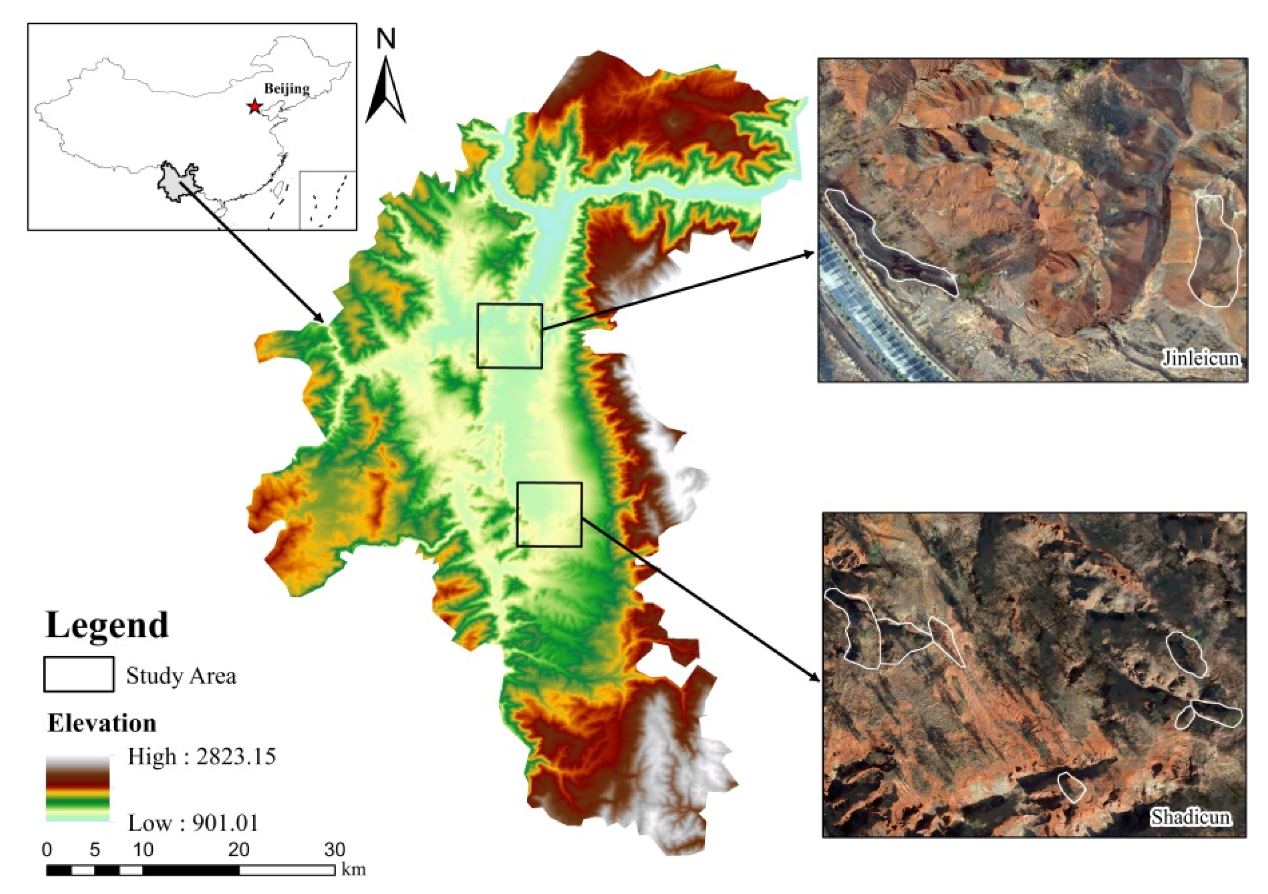
2.1. Study Area

The study area is located in Yuanmou County, Yunnan province of China, which is a typical representation of the Jinsha dry-hot valley region. The study region covers an area of 2020 km², extending from 101°35′ E to 102°06′ E and from 25°23′ N to 26°06′ N (Figure 1). The study area has a subtropical monsoon climate and is characterized by a dry-hot climate, concentrated rainfall, and notable dry and wet seasons [41,49,50]. The annual average temperature is approximately 21.9°C, and the annual precipitation is about 615 mm. In this area, the dry and wet seasons are clear and distinct. The rainy season lasts from May to October, which provides about 91% of the annual precipitation, and heavy showers and rainfall are common in the rainy season. However, precipitation in the dry season only accounts for about 9% of the annual precipitation. Moreover, the potential evaporation can be as high as 6.4 times the annual precipitation, which results in a year-round dry climate in this area. Dominant soils in the region are dry, red soil and vertisols, with a mean dry bulk density of 1.4 to 1.8 g·cm⁻³ [51]. The zonal vegetation type in the area is tropical bushveld with scattered trees, which results in a tropical savanna-like ecosystem whose forest coverage rate is as low as 3.4~6.3% [52,53]. The dominant species are Heteropogon contortus and Dodonaea riscosa [52]. In addition, the stratum belongs to the Quaternary lacustrine sediments, which feature poor structures, low water infiltration rates, and high soil-erosion rates. Therefore, gully erosion is acute in the area, with an average gully density of 4.5 km·km⁻² and a maximum density of 7.4 km·km⁻², and the soil erosion modulus amounts to 8000~20000 t·km⁻²·a⁻¹ [54,55,56].

2.2. Data Collection and Division of the Gully Development Stage

A series of detailed field investigations on gully erosion was conducted in the Yuanmou dry-hot valley region from 2013 to 2014. Based on these investigations, about 134 gullies with typical development features were chosen in this study (Figure 1), among which 111 gullies were used to establish the prediction model of gully volume, and the other 23 gullies were used to validate the effectiveness and accuracy of the established model. The detailed geomorphic information of 134 gullies was surveyed by using a total station (Leica TCR802POWER). Intervals between the measurement points were mostly less than 0.5 m along the gully sidewall and bed. Some complementary points were measured with a Trimble GPS to eliminate high RMS error points. The Digital Elevation Model (DEM) is regarded as an effective method to obtain terrain information, and many geomorphological analysis methods have been developed based on DEM [57]. Thus, a DEM with 0.1 m resolution for each gully was created using the Radial Basis Function (RBF) [58] based on the measured points (Figure 2). The ME and RMSE of DEMs ranged from −0.191 to 0.152 and from 0 to 1.212, respectively.

According to the DEM, morphological parameters, such as the gully length (L, m), gully width (W, m), gully depth (D, m), gully cross-section area (A, m²), gully volume (V, m³), gully vertical gradient (Vg), and breadth–depth ratio (Bd), were derived and calculated using the 3D analyst and spatial analyst tools. In addition, the mean values of the morphological parameters were computed to characterize the systematic features of the gully. The data in this paper for the morphological parameters are presented as mean values, whose detailed computing methods are described in

Table 1. The computing methods for the morphological parameters of the gully.

Morphological Parameters of the Gully	Computing Method
Length (L, m)	Measure the length along the bottom line of the gully bed. If there are channel branches in the gully, the longest branch will be regarded as the length of the gully.
Width (W, m), Depth (D, m), Cross-section area (A, m2)	Measure the width, depth, and cross-section area every 2 m along the extension direction of the gully and then calculate the mean value.
Volume (V, m3)	Calculate the gully volume directly based on the DEM.
Vertical gradient (Vg)	$Vg=\Delta H/L$, where $\Delta H$ is equal to the elevation difference between the gully head and gully bottom.
Breadth–depth ratio (Bd)	$Bd=W/D$

.

Geomorphic information entropy (E_gi) was then calculated to evaluate the development degree of gully erosion, according to the study results of Ai [59], Sidorchuk [60], and Zhang et al. [61]. In a channel system, the value of E_gi reflects the activity degree of the gully; the smaller the value of E_gi is, the more intense the erosion activity is, and vice versa. Thus, in this study, the larger the value of E_gi was, the less intense the erosion activity was, thereby indicating that the gully tended to be stable [42]. The calculation formula is as follows:

$$E_{gi}=S-1-\ln S={\displaystyle \underset{0}{\overset{1}{\int }}f(x)}dx-1-\ln [{\displaystyle \underset{0}{\overset{1}{\int }}f(x)}dx]$$

(1)

where E_gi is geomorphic information entropy, S is the integral value of Strahler area elevation, and f(x) is the fitting function of Strahler area elevation.

Based on the geomorphic information entropy theory, Ai [59] divided the development degree of landform erosion into three phases. When E_gi < 0.1110, the development degree of landform erosion is in the young stage; when 0.1110 ≤ E_gi ≤ 0.4000, the development degree of landform erosion is in the mature stage; when E_gi > 0.4000, the development degree of landform erosion is in the old stage. The dividing standard is to some extent universal but can vary with the difference in regional geographical factors in practical applications [62]. In this study, the value of E_gi was between 0.059 and 0.290. According to the standard of Ai [59] for geomorphic information entropy, the 134 gullies were all in the young and mature stages, but this result was not consistent with the observed gully development stage in the field. Therefore, this study considered all of the geomorphic features, vegetation conditions, and deposits in the gullies to redefine the division standard for the gully development stage. The detailed division standard is shown in

Table 2. The division standard for the gully development stage.

Gully Development Stage	Values of Egi	Geomorphic Features, Vegetation Condition, and Deposits in Gullies
Very active	Egi < 0.1110	High and steep gully wall with some concave holes; no or very little vegetation and deposits in the gully bed
Active	0.1110 ≤ Egi < 0.1500	High and steep gully wall with some concave holes; gully bed covered with a little vegetation and deposits
Relatively active	0.1500 ≤ Egi < 0.2000	Gentle gully wall without apparent concave holes; gully bed with some vegetation and deposits
Slightly stable	Egi ≥ 0.2000	Low and gentle gully wall; gully bed covered with some vegetation and deposits

.

2.3. Construction and Effectiveness Test of Empirical Models

A nonlinear regression analysis was used to determine the relationships between gully volume and other morphological parameters, and the corresponding empirical models were established according to the results of statistical analyses carried out using SPSS 16.0 and Origin 8.0. In addition, the graphs in this study were drawn with the Sigma Plot software (version 10.0).

The morphological features in 23 other gullies were extracted to test the effectiveness of constructed empirical models. First, a t-test was used to evaluate the significance of the differences between the average of the measured and estimated gully volume [63]. In addition, the average relative error (E_r) [39] and Nash efficiency coefficient (E_ns) [64], as well as the R² of the linear regression between the measured and evaluated gully volume, were calculated to test the effectiveness of models.

The E_r can examine the accuracy of the mathematic model; the calculation formula is provided as Equation (2). The E_ns was used as an indicator to evaluate the goodness of fit of the model and varied from −∞ to 1; the calculation formula is provided as Equation (3). E_ns = 1 indicates a perfect match between the measured value and the simulated value of the model; E_ns = 0 indicates that the result of the model simulation is equal to the average series of the measured value; Ens < 0 indicates that the measured average value was better than the simulated value.

$$E_r=\frac{1}{n}{\Sigma }_{i=1}^n\left|\frac{M_i-P_i}{M_i}\right|$$

(2)

$$E_{ns}=1-\frac{{\Sigma }_i^n{\left(M_i-P_i\right)}^2}{{\Sigma }_i^n{\left(M_i-M_{ave}\right)}^2}$$

(3)

where i representes the number of gullies, M_i is the measured volume of the gully i, P_i is the predicted volume of the gully i, and M_ave is the average value of the measured volume.

3. Results

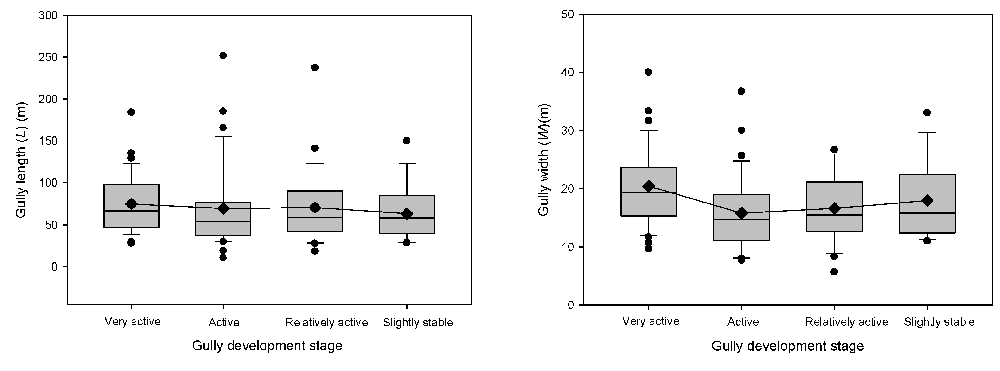
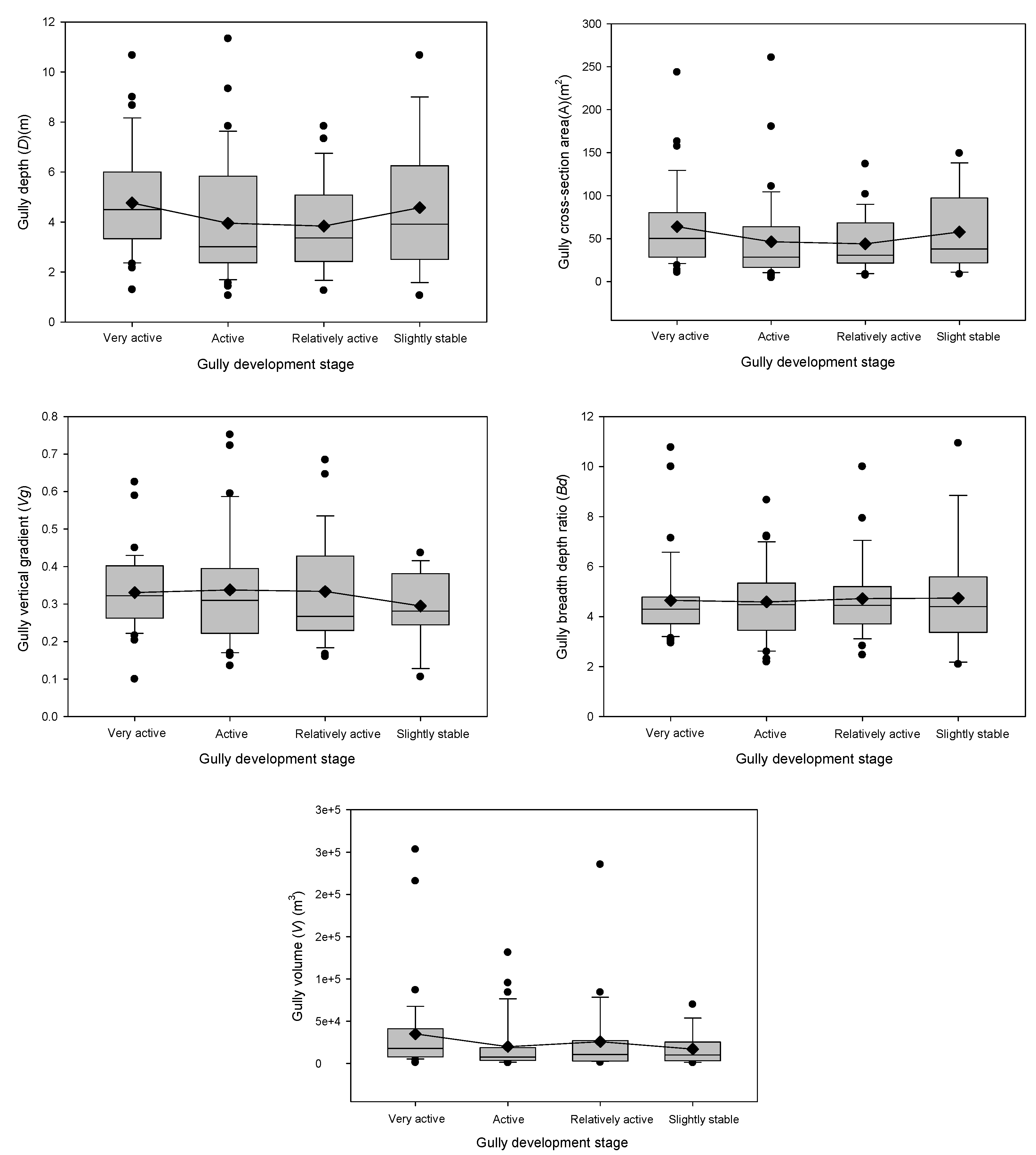
3.1. Morphological Features of Gully

The gully length (L, m), width (W, m), depth (D, m), cross-section area (A, m²), volume (V, m³), vertical gradient (Vg), and breadth–depth ratio (Bd) were considered in this work as the basic morphological features of the gully and showed some differences between different gully development stages. The variation in gully length, width, depth, cross-section area, vertical gradient, breadth–depth ratio, and volume between different developmental stages are shown in Figure 3. Except for the breadth–depth ratios of the gullies, the means and medians of the other six morphological characteristic parameters generally decreased with a decrease in the activity degree of the gully. For gully length and volume, there were obvious reduction trends when gullies tended to be stable, and the average decrease rate for gully length ranged from 2.164 (for the median) to 3.313 (for the mean), and the decrease rate for gully volume ranged from 2067.900 (for the median) to 4789.800 (for the mean). The underlying reason for this result may be that the deposits accumulated gradually from the end of the gully channel to the head and at the same as the vegetation was settling in the gullies. For gully width, depth, and cross-section area, there were turning points for their means, medians and the 10th, 25th, 75th, and 90th percentiles in the stable processes of gullies, which indicated that the diminishing processes of gully width, depth, and cross-section area were not continuous when the gullies changed from (relatively) active to slightly stable. However, the discontinuous decrease in gully width, depth, and cross-section area did not change the overall situation where the gullies tended to be stable, which may because the lateral and vertical erosion phenomena in the gullies remained active along with the deposits accumulating at the end of the gully. Moreover, the effect of the deposition process was more intensive than that of lateral and vertical erosion. For this reason, the gully width, depth, and cross-section area experienced a slight increase, but these processes did not interrupt the stable progression of the gully.

In addition, the means of the gully vertical gradients in the very active, active, and relatively active stage did not show obvious differences but were significantly larger than those in the slightly stable stage, possibly because the micro-topographies of the gullies in the slightly stable stage were relatively flat compared to those of the other three stages. Moreover, the flat micro-topographies of gullies in the slightly stable stage were the result of deposits accumulating in the gully channels. Finally, there was an increasing trend for the breadth–depth ratio of the gully along with weakness in the active degree of the gully for the mean, median, and 75th and 90th percentiles. This phenomenon was very easy to understand because gullies in the stable stage usually tended to be U-shape, had a larger width and smaller depth, and a correspondingly greater breadth–depth ratio. In contrast, although both the widths and depths of the gullies experienced increases when the gullies moved from relatively active stage to the slightly stable stage, the breadth–depth ratios of gullies in the slightly stable stage notably increased compared to the previous three development stages of the gullies. These demonstrate that a separate change in a gully’s width or depth might have a very minimal effect on the evolution development stage of the gully.

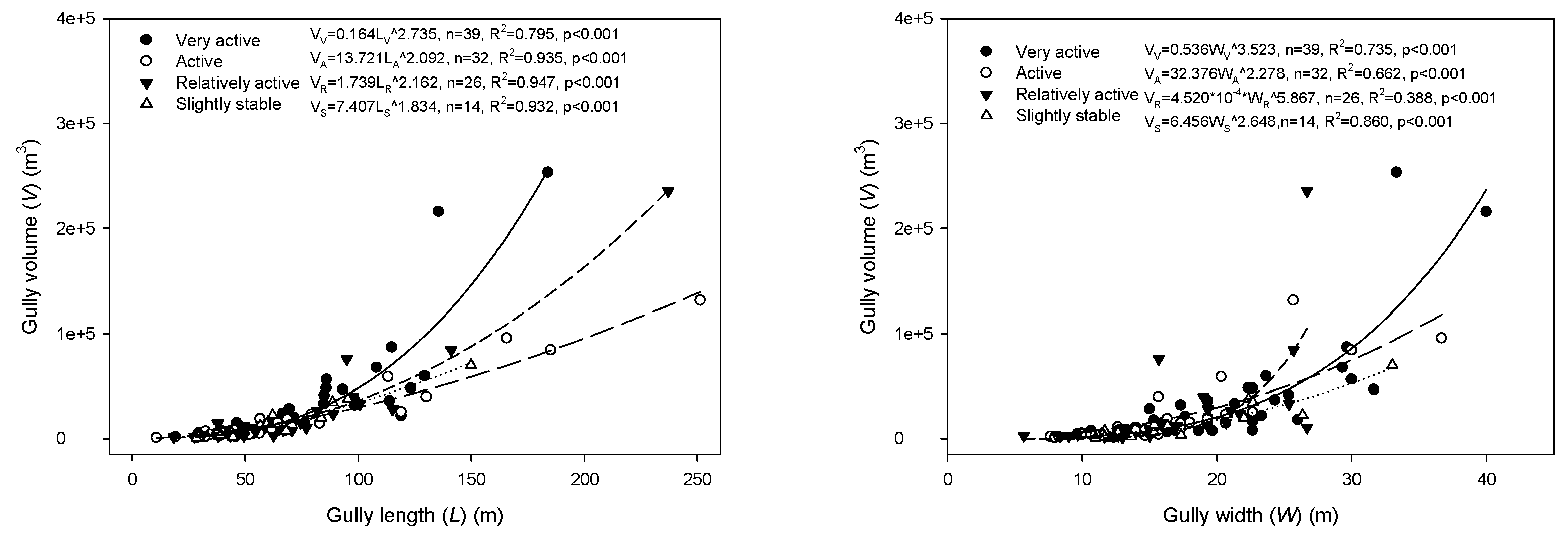
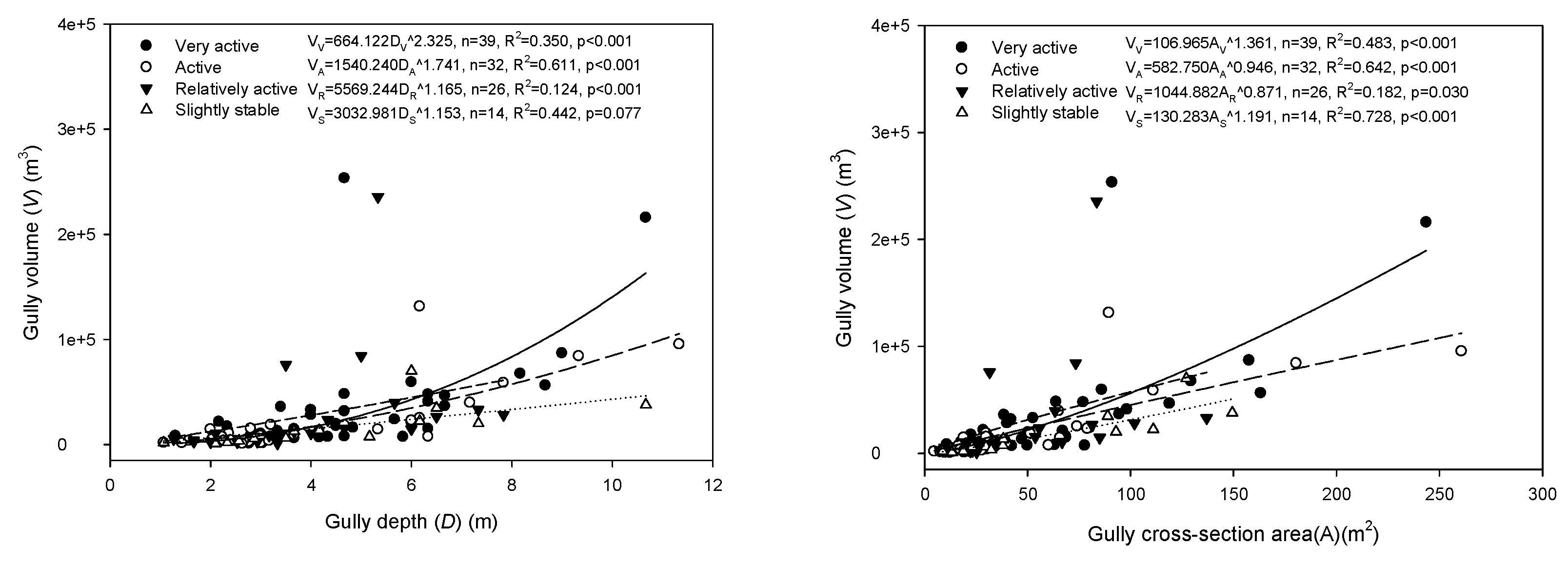
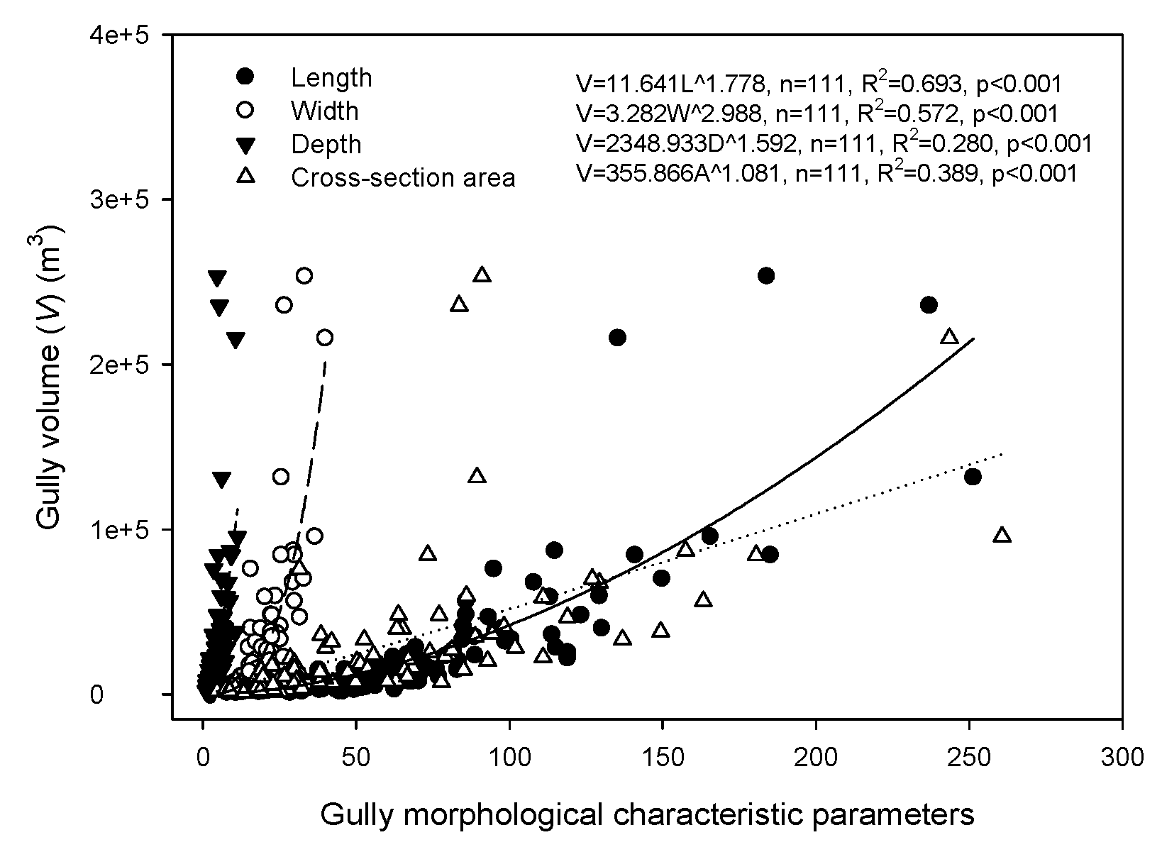
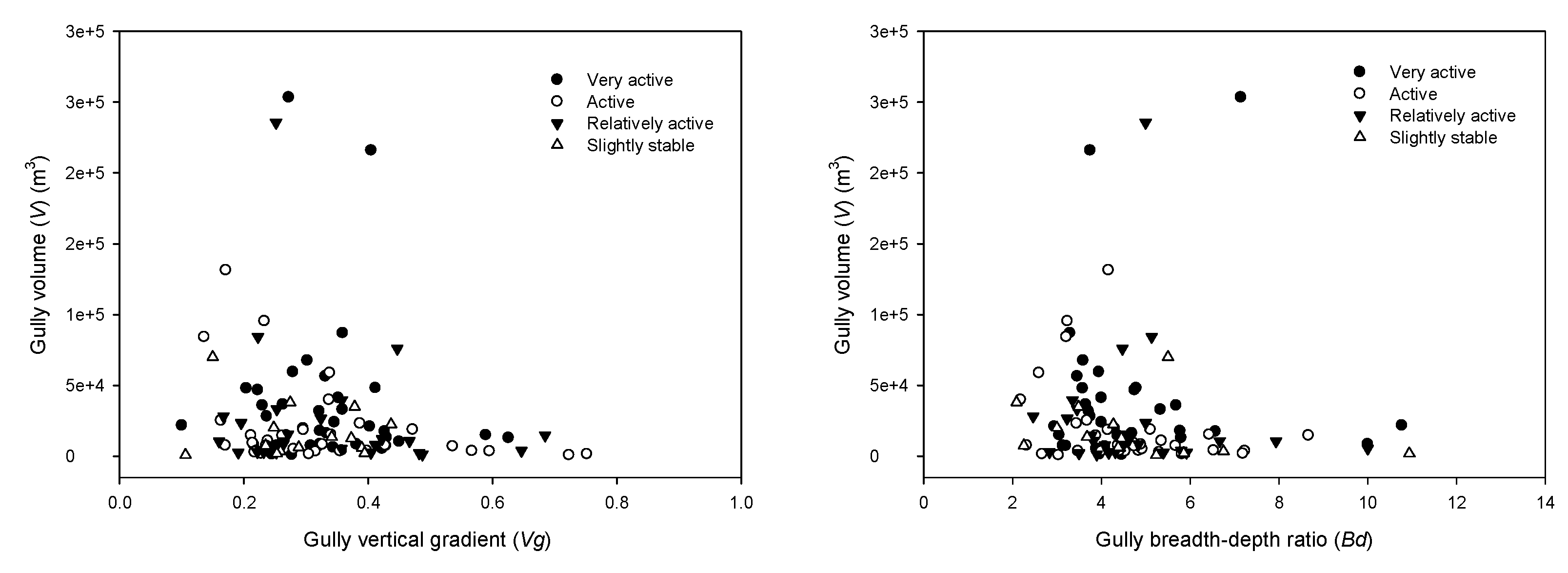
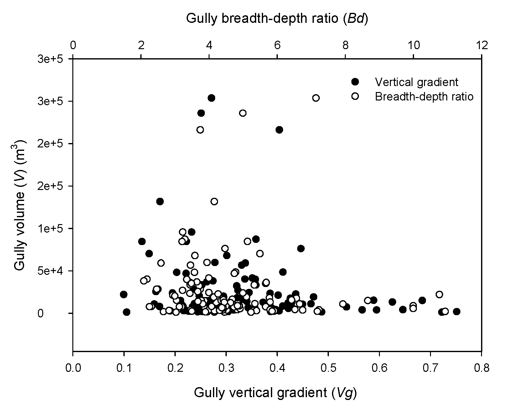
3.2. Relationship between the Different Morphological Features of Gullies

Gully volume is a direct index that can reflect the eroded degree and soil loss of the land surface. Exploring the internal relationship between gully volume and other morphological features can not only predict soil loss through gully volume when there is a lack of directly measured data but can also verify the precision of measured gully volume when such measurements exist.

Figure 4 illustrates the relationship between gully volume and gully length, width, depth, and cross-section area in different gully development stages. Overall, there was a significant correlation between the aforementioned gully morphological features, and a series of power functions was built to reflect the mathematical relationship between each feature. For gullies in very active and active stages, all eight fitting equations of V-L, V-W, V-D, and V-A reached an extremely significant level (p < 0.001). However, the corresponding determinate coefficient R² were not at the same level. In the very active stage, the R² of the fitting equations for V-L and V-W were larger than 0.75, which indicates that the fitting equation was able to accurately reflect the internal relationship among gully volume and gully length and gully width. In contrast, in the active stage, only the R² of the fitting equation for V-L was larger than 0.75, while the R² values of the other three fitting equations for V-W, V-D, and V-A were less than 0.75, which indicates that gully volume in the active stage can only be accurately predicted by gully length. For gullies in the relatively active stage, the fitting equations of V-L, V-W, and V-D reached an extremely significant level (p < 0.001), but the fitting equation of V-A was only significant at a level of 0.05 (p = 0.03 < 0.05, but >0.01). In addition, the R² values of the fitting equations for V-W, V-D, and V-A were very small (all < 0.5); only the R² value of V-L was larger than 0.75 (R² = 0.947). In the slightly stable stage, the fitting equation of V-D was not significant (p = 0.077 > 0.05), and the R² values of the fitting equations for V-L and V-W were larger than 0.75. Thus, wherever in all development stages of the gully, there was a good fitting relationship between gully volume and gully length. Only in the very active and slightly stable stages was there a good fitting relationship between gully volume and gully width. However, we did not detect a good fitting relationship between gully depth, cross-section area, and gully volume.

The corresponding fitting equations were calculated, as shown in Figure 5, to determine the relationship between gully volume and the other parameters under all development stages. There were extremely significant power functions between gully volume and gully length, width, depth, and cross-section area when all 111 gullies were considered. The R² values of the four fitting equations were all less than 0.75; only the R² values of the equation V-L was close to 0.75. These results indicate that gully length is a more effective and accurate morphological feature for predicting gully volume than gully width, depth, or cross-section area.

As the vertical gradient and breadth–depth ratio are also important basic morphological features of gullies, regression analyses were conducted among the gully volume and the vertical gradient and the breadth–depth ratio (Figure 6 and Figure 7). No significant fitting function could be found in any development stage of the gully (i.e., the very active, active, relatively active, slightly stable stages) or the overall process of gully development. Overall, we observed significant relationships between gully volume and gully length, width, depth, and cross-section area but found no similar relationship between gully volume and vertical gradient or the breadth–depth ratio. Meanwhile, gully length and width, especially gully length, were found to be the best indicators to predict gully volume among the various morphological characteristic parameters.

3.3. Verification of the Constructed Empirical Models

In the above analysis, empirical models were established between gully volume and other morphological features, and p and R² values of the fitting equation were used to determine the correctness of the models. We found that the models of V-L and V-W were better than the others. However, to what extent these models are valid requires further verification. Gully volume was predicted according to the established empirical models by using gully length, width, depth, and cross-section area values extracted from the DEMs of 23 other typical gullies in our study area to validate the empirical models. In addition, the gully volumes of the 23 gullies were measured directly via their DEMs, and then a comparative analysis between the predicted and measured gully volume was conducted. First, a t-test was used to analyze the differences between the average of the measured and predicted gully volumes. The results showed that there was no significant difference between the two volumes at a level of 0.01 because all values of p were larger than 0.01, which indicates that the variances in the measured and predicted gully volumes were equal and that the empirical models constructed in this study were valid basically (

Table 3. Results of the validity test for estimation models of gully volume.

Gully Development Stage *	Number of Gullies Used for Verification	Prediction Model ***	Indexes for Validity Test
			Er	Ens	R2	p **
Relatively active	21	V-L	0.455	0.840	0.845	0.894
		V-W	1.239	−7.127	0.185	0.822
		V-D	3.077	−0.268	0.577	0.034
		V-A	5.333	−1.696	0.708	0.027
Slightly stable	2	V-L	0.794	0.943	1	0.446
		V-W	0.701	0.965	1	0.273
		V-D	7.564	−0.270	1	0.417
		V-A	0.465	0.990	1	0.864
All (Relatively active + Slightly stable)	23	V-L	1.869	0.072	0.822	0.036
		V-W	2.410	−9.812	0.288	0.324
		V-D	2.434	0.558	0.592	0.487
		V-A	1.966	0.483	0.705	0.607

Notes: * The 23 gullies used to verify the models were all in the relatively active and slightly stable stages according to the values of E_gi among the 23 gullies. ** The significance value of the t-test for measured and predicted gully volume. *** The specific prediction models can be found in Figure 4 and Figure 5.

).

To further test the effectiveness of the above-mentioned models of V-L, V-W, V-D, and V-A in different gully development stages, the average relative error (E_r), Nash efficiency coefficient (E_ns), and R² of the linear regression between the measured and predicted gully volume were calculated (Table 3). According to previous studies, the smaller the value of E_r was, the better the prediction model was. In contrast, the larger the value of E_ns and R² were, the better the prediction model was. Therefore, it was determined that the model of V-L can predict gully volume better than the models of V-W and V-D in all developmental stages of a gully when E_r is regarded as the unique judgment criterion. In addition, the effectiveness of the model of V-A was better than that of V-L in the slightly stable stage when only comparing the values of E_r.

However, when comparing the values of E_ns in different models, some differences were observed. The results showed that there are different optimal models for predicting gully volume in different gully development stages. In the relatively active stage, the model of V-L performed best with an E_ns of 0.840, which was significantly larger than the E_ns values in the models of V-W and V-D. In the slightly stable stage, the best choice was the model of V-A, whose E_ns was 0.990. Furthermore, the model of V-D was best with an E_ns of 0.558 when all of the gullies (including those in relatively active stage and slightly stable stage) were considered in the model.

The R² value of the fitting equation was an important indicator to assess the goodness of fit. In the relatively active stage, the model of V-L performed best with an R² value of 0.845, which was larger than the R² value in the models of V-W, V-D, and V-A. In addition, the R² of the model of V-L was equal to 0.822, which was noticeably larger than the R² values in the other three models when all 23 gullies were taken into account. As only two gullies were used to verify the model in the slightly stable stage, the R² value of the fitting curve was always 1.000. Consequently, the R² could not be used to evaluate the effectiveness of the models in this stage. Therefore, the model of V-L was better in predicting gully volume compared to the models of V-W, V-D, and V-A when R² was regarded as the only judgment indicator.

In conclusion, the best prediction model for gully volume changes to some degree when different evaluation indexes are used. In this study, when all the E_r, E_ns, and R² values of the prediction models were taken into account, the predictive effect of the model of V-L was shown to be the best among the four verified models. The best prediction models for gully volume based on the results of the regression analyses between gully volume and other morphological features are shown in

Table 4. The optimization models for predicting gully volume in different development stages of gullies.

Gully Development Stage	Prediction Model	N	R2	p
Very active	$V=0.164L^{2.735}$	39	0.795	<0.01
Active	$V=13.721L^{2.092}$	32	0.935	<0.01
Relatively active	$V=1.739L^{2.162}$	26	0.947	<0.01
Slightly stable	$V=7.407L^{1.834}$	14	0.932	<0.01
Whole	$V=11.641L^{1.778}$	111	0.693	<0.01

. Notably, the best prediction models for gully volume were validated based only on the 23 gullies in the relatively active and slightly stable stages because the number of eligible gullies was limited when taking into account the heterogeneity of the terrain that must be controlled to a certain extent and the possibility of measuring the relevant gullies. Nevertheless, the results in this study still have significance in facilitating gully volume prediction and guiding gully erosion control and ecological restoration in the Jinsha dry-hot valley region.

4. Discussion

4.1. Identification of Gully Development Stage

In this study, the morphological features of gullies were described, the relationship between gully volume and other morphological characteristic parameters was discussed, and predictive models for gully volume were established based on about 111 gullies in the Jinsha dry-hot valley region. Furthermore, the effectiveness of predictive models was verified according to the investigative results of 23 other gullies in our study area, and the model of V-L was shown to be the best. Importantly, this study adapted geomorphic information entropy (E_gi) as a division standard to determine the development stage of gullies, and this standard was very effective in distinguishing different gullies. Although geomorphic information entropy (E_gi) is usually used to divide geomorphic development processes, there is still no universal standard with definite critical values. For example, Wang et al. [65] proposed a different geomorphologic classification standard by adjusting the standard established by Ai [39]. In addition, Xie et al. [66] put forward a classification standard for the catchment geomorphologic development stage based on geomorphic information entropy in Tianshan, China, which was different from the standard proposed by Ai [59] and the standard proposed by Wang et al. [65]. The underlying reason for these differences is that the relevant geomorphic development processes are very complex and full of heterogeneity, as they are affected by geomorphology, climate, hydrology, vegetation, soil type, and even human activities. Therefore, the specific criteria used to divide the geomorphic developmental process based on geomorphic information entropy should be adjusted dynamically according to the specific situation of each study area. For these reasons, the uniqueness of the study area and the land surface features of the studied gullies were comprehensively considered alongside previous research results, and the division standard based on geomorphic information entropy (E_gi) was determined as shown in Table 2. Although a good result was achieved in this study based on the division results of the developmental stages of gullies, our standard might still have some limitations when applied in other regions. However, this limitation is universal. Therefore, determining a general standard that is suitable for dividing the geomorphic development process will remain an ongoing area of study for our research group and for other scholars who are interested in geomorphic development and evolution. Notably, due to the differences in geographical conditions, it is unrealistic to establish a unique and fixed classification standard worldwide, but it may be feasible to establish a series of classification standards based on the same or similar geographical conditions, including topography, climate, hydrology, etc. It will be necessary to collect and compare studies on topographical classification from all around the world to achieve this goal.

4.2. The Meaning of the Model Parameters

A series of regression analyses were conducted in this study to explore the relationship between gully volume and other morphological features. The results showed that the power functions were able to reflect these internal relationships very well, which was consistent with previous studies [6,34,35,63,67]. In addition, in a power function of V = aL^b, parameter a is usually regarded as an indicator that reflects the degree of correlation between L and V. The greater the absolute value of a is, the stronger the correlation between the two will be. Parameter b is an indicator that reflects the growth or decrease rate of V when a unit change occurs in variable L. In this study, the relationships between gully volume and gully length, width, depth, and cross-section area were discussed, and the model of V-L was shown to be the best. In the model of V-L, the value of a ranged from 0.164 to 13.721, while the value of b changed from 1.778 to 2.735, which was very different from the results of other regions around the world. For example, Li [67] found a power function between gully volume and length with the form of V = aL^b, and the values of a and b, respectively, ranged from 0.653 to 0.899 and from 1.990 to 2.162 in the Loess Plateau region. Kompani-Zare et al. [6] calculated the mathematical relationship between gully volume and length in 146 gullies in Fars Province, Iran, and found a power function between the two factors; and the parameters of a and b were in the ranges of 1.0–10.8 and 0.8–1.4. Nachtergaele et al. [35], Capra et al. [63], and Zucca et al. [34] also found power functions able to accurately reflect the relationship between gully volume and length in Spain, Portugal, and Italy, respectively, but the values of both a and b varied considerably. The value of parameter a ranged from 0.008 to 0.114, and that of parameter b varied from 0.920 to 1.420. These results indicate that the values of parameters a and b experience an evident change from region to region. At the same time, the scale of the gully was an extremely important factor that affected the values of parameters a and b. In the studies of Kompani-Zare et al. [6], Zucca et al. [34], Nachtergaele et al. [35], and Capra et al. [63], the gullies were ephemeral with relatively small scales (gully volume < 100 m³, length < 60 m, cross-section area < 0.5 m², width < 2 m). In contrast, the gullies observed by Li [67] were permanent with scales that were usually obviously larger than those of ephemeral gullies. In addition, the gullies in this study were also permanent, and the gully scale in our study was larger than that in the study of Li [67]. Therefore, the values of parameters a and b had a positive correlation with the scale of the gullies. Additionally, unlike the value of parameter a, which varied obviously at different channel scales of gullies, the value of parameter b varied only slightly. These results suggested that the channel scale of a gully affects not only the strength of the correlation between V and L but also the increased rate of V with L, although the degree influenced by the channel scale of gully may be different. Last, all our prediction models were constructed based on the empirical regression method, which offers obvious advantages in handling nonlinear relationships between two factors and linear relationships among multiple variables. However, the morphological features of gullies can be affected or even determined by some other factors for which the influencing mechanism are not very clear, such as soil type, land utilization type, and human disturbances. For analyzing the relationship between such variables and attempting to predict gully erosion based on the analysis results, artificial intelligence technology, especially machine learning models, can perform very well [68,69]. To improve our prediction model for gully volume, more influencing factors will be considered in the future, and machine learning models, including random forest and the support vector machine model [43], will be a priority.

5. Conclusions

In this work, the change processes for the morphological features of gullies, including gully length, width, depth, cross-section area, volume, vertical gradient, and breadth–depth ratio, were analyzed between different gully development stages. Moreover, the relationship between gully volume and other morphological features was explored, and corresponding empirical models for predicting gully volume were constructed. In addition, this study verified the effectiveness of the models, and optimized prediction models for gully volume were selected. The results showed that the mean value of gully morphological characteristic parameters (including gully length, width, depth, cross-section area, volume, and vertical gradient) decreased with a weakness in the activity degree of the gully, although the decrease processes differed among parameters. Significant regression relationships were detected between gully volume and other morphological features, and a series of empirical models in the form of a power function to predict gully volume was constructed. Compared with the other morphological characteristic parameters, gully length and width, especially gully length, proved to be the best indicators for predicting gully volume. The effectiveness test of all these empirical models showed that the model of V = aL^b (in the very active stage a = 0.164, b = 2.735; in the active stage a = 13.721, b = 2.092; in the relatively active stage a = 1.739, b = 2.162; in the slightly stable stage a = 7.407, b = 1.834; in whole process a = 11.641, b = 1.778) was the most effective in predicting gully volume in the Jinsha dry-hot valley region. These results will provide a theoretical reference for identifying the gully development stage and predicting the gully volume with basic morphological features. Moreover, establishing an empirical prediction model for gully volume can provide basic guidance for the remediation of gullies in the Jinsha dry-hot valley region. A universally applicable prediction model for gully volume and gully erosion that considers comprehensive influencing factors will be the subject of our future research.

References

1. Douglas-Mankin, K.R.; Roy, S.K.; Sheshukov, A.Y.; Biswas, A.; Gharabaghi, B.; Binns, A.; Rudra, R.; Shrestha, N.K.; Daggupati, P. A comprehensive review of ephemeral gully erosion models. Catena 2020, 195, 104901. [Google Scholar] [CrossRef]
2. Mor-Mussery, A.; Laronne, J.B. The effects of gully erosion on the ecology of arid loessial agro-ecosystems, the northern Negev, Israel. Catena 2020, 194, 104712. [Google Scholar] [CrossRef]
3. Poesen, J.; Nachtergaele, J.; Verstraeten, G.; Valentin, C. Gully erosion and environmental change: Importance and research needs. Catena 2003, 50, 91–133. [Google Scholar] [CrossRef]
4. Poesen, J.W.A.; Hooke, J.M. Erosion, flooding and channel management in Mediterranean environments of southern Europe. Prog. Phys. Geogr. 1997, 21, 157–199. [Google Scholar] [CrossRef]
5. Vandekerckhove, L.; Poesen, J.; Wijdenes, D.O.; Gyssels, G.; Beuselinck, L.; Luna, E.D. Characteristics and controlling factors of bank gullies in two semi-arid mediterranean environments. Geomorphology 2000, 33, 37–58. [Google Scholar] [CrossRef]
6. Kompani-Zare, M.; Soufi, M.; Hamzehzarghani, H.; Dehghani, M. The effect of some watershed, soil characteristics and morphometric factors on the relationship between the gully volume and length in Fars Province, Iran. Catena 2011, 86, 150–159. [Google Scholar] [CrossRef]
7. Candido, B.M.; James, M.; Quinton, J.; De Lima, W.; Naves Silva, M.L. Sediment source and volume of soil erosion in a gully system using UAV photogrammetry. Rev. Bras. Cienc. Do Solo 2020, 44, e0200076. [Google Scholar] [CrossRef]
8. Kaiser, A.; Neugirg, F.; Rock, G.; Mueller, C.; Haas, F.; Ries, J.; Schmidt, J. Small-scale surface reconstruction and volume calculation of soil erosion in complex moroccan gully morphology using structure from motion. Remote Sens. 2014, 6, 7050–7080. [Google Scholar] [CrossRef] [Green Version]
9. Woodward, D.E. Method to predict cropland ephemeral gully erosion. Catena 1999, 37, 393–399. [Google Scholar] [CrossRef]
10. Casalí, J.; López, J.J.; Giráldez, J.V. Ephemeral gully erosion in southern Navarra (Spain). Catena 1999, 36, 65–84. [Google Scholar] [CrossRef]
11. Zhu, T.X. Gully and tunnel erosion in the hilly Loess Plateau region, China. Geomorphology 2012, 153–154, 144–155. [Google Scholar] [CrossRef]
12. Castillo, C.; Perez, R.; James, M.R.; Quinton, J.N.; Taguas, E.V.; Gomez, J.A. Comparing the accuracy of several field methods for measuring gully erosion. Soil Sci. Soc. Am. J. 2012, 76, 1319–1332. [Google Scholar] [CrossRef] [Green Version]
13. Vandekerckhove, L.; Poesen, J.; Wijdenes, D.O.; Gyssels, G. Short-term bank gully retreat rates in Mediterranean environments. Catena 2001, 44, 133–161. [Google Scholar] [CrossRef]
14. Hessel, R.; van Asch, T. Modelling gully erosion for a small catchment on the Chinese Loess Plateau. Catena 2003, 54, 131–146. [Google Scholar] [CrossRef]
15. Capra, A.; Scicolone, B. Ephemeral gully erosion in a wheat-cultivated area in Sicily (Italy). Biosyst. Eng. 2002, 83, 119–126. [Google Scholar] [CrossRef]
16. You, Z.M.; Wu, Y.Q.; Liu, B.Y. Study of monitoring gully erosion using GPS. J. Soil Water Conserv. 2004, 18, 91–94. [Google Scholar]
17. Chen, Y.; Jiao, J.; Wei, Y.; Zhao, H.; Yu, W.; Cao, B.; Xu, H.; Yan, F.; Wu, D.; Li, H. Accuracy Assessment of the Planar Morphology of Valley Bank Gullies Extracted with High Resolution Remote Sensing Imagery on the Loess Plateau, China. Int. J. Environ. Res. Public Health 2019, 16, 369. [Google Scholar] [CrossRef] [Green Version]
18. Wells, R.R.; Momm, H.G.; Bennett, S.J.; Gesch, K.R.; Dabney, S.M.; Cruse, R.; Wilson, G.V. A measurement method for rill and ephemeral gully erosion assessments. Soil Sci. Soc. Am. J. 2016, 80, 203–214. [Google Scholar] [CrossRef]
19. Casali, J.; Loizu, J.; Campo, M.A.; De Santisteban, L.M.; Alvarez-Mozos, J. Accuracy of methods for field assessment of rill and ephemeral gully erosion. Catena 2006, 67, 128–138. [Google Scholar] [CrossRef]
20. Kociuba, W.; Janicki, G.; Rodzik, J.; Stepniewski, K. Comparison of volumetric and remote sensing methods (TLS) for assessing the development of a permanent forested loess gully. Nat. Hazards 2015, 79, S139–S158. [Google Scholar] [CrossRef]
21. Marzolff, I.; Poesen, J. The potential of 3D gully monitoring with GIS using high-resolution aerial photography and a digital photogrammetry system. Geomorphology 2009, 111, 48–60. [Google Scholar] [CrossRef]
22. Ries, J.B.; Marzolff, I. Monitoring of gully erosion in the Central Ebro Basin by large-scale aerial photography taken from a remotely controlled blimp. Catena 2003, 50, 309–328. [Google Scholar] [CrossRef]
23. Gimenez, R.; Marzolff, I.; Campo, M.A.; Seeger, M.; Ries, J.B.; Casali, J.; Alvarez-Mozos, J. Accuracy of high-resolution photogrammetric measurements of gullies with contrasting morphology. Earth Surface Process. Landf. 2009, 34, 1915–1926. [Google Scholar] [CrossRef]
24. Gomez-Gutierrez, A.; Schnabel, S.; Berenguer-Sempere, F.; Lavado-Contador, F.; Rubio-Delgado, J. Using 3D photo-reconstruction methods to estimate gully headcut erosion. Catena 2014, 120, 91–101. [Google Scholar] [CrossRef]
25. Gulam, V.; Gajski, D.; Podolszki, L. Photogrammetric measurement methods of the gully rock wall retreat in Istrian badlands. Catena 2018, 160, 298–309. [Google Scholar] [CrossRef]
26. Romanescu, G.; Cotiuga, V.; Asandulesei, A.; Stoleriu, C. Use of the 3-D scanner in mapping and monitoring the dynamic degradation of soils: Case study of the Cucuteni-Baiceni Gully on the Moldavian Plateau (Romania). Hydrol. Earth Syst. Sci. 2012, 16, 953–966. [Google Scholar] [CrossRef] [Green Version]
27. Zhang, P.; Zheng, F.L.; Wang, B.; Chen, J.Q.; Ding, X.B. Comparative study of monitoring gully erosion morphology change process by using high precision GPS, Leica HDS 3000 Laser Scanner and Needle Board Method. Bull. Soil Water Conserv. 2008, 28, 11–15, 20. [Google Scholar]
28. Alfonso-Torreno, A.; Gomez-Gutierrez, A.; Schnabel, S.; Lavado Contador, J.F.; De Sanjose Blasco, J.J.; Sanchez Fernandez, M. sUAS, SfM-MVS photogrammetry and a topographic algorithm method to quantify the volume of sediments retained in check-dams. Sci. Total Environ. 2019, 678, 369–382. [Google Scholar] [CrossRef] [PubMed]
29. Gong, C.G.; Lei, S.G.; Bian, Z.F.; Liu, Y.; Zhang, Z.A.; Cheng, W. Analysis of the development of an erosion gully in an open-pit coal mine dump during a winter freeze-thaw cycle by using low-cost UAVs. Remote Sens. 2019, 11, 1356. [Google Scholar] [CrossRef] [Green Version]
30. Mihai, N.; Mihai, C.M.; Paolo, T. Using UAV and LiDAR data for gully geomorphic changes monitoring. Dev. Earth Surface Process 2020, 23, 271–315. [Google Scholar]
31. Frankl, A.; Stal, C.; Abraha, A.; Nyssen, J.; Rieke-Zapp, D.; De Wulf, A.; Poesen, J. Detailed recording of gully morphology in 3D through image-based modelling. Catena 2015, 127, 92–101. [Google Scholar] [CrossRef] [Green Version]
32. Garosi, Y.; Sheklabadi, M.; Conoscenti, C.; Pourghasemi, H.R.; Van Oost, K. Assessing the performance of GIS-based machine learning models with different accuracy measures for determining susceptibility to gully erosion. Sci. Total Environ. 2019, 664, 1117–1132. [Google Scholar] [CrossRef]
33. Siljeg, A.; Domazetovic, F.; Maric, I.; Loncar, N.; Panda, L. New method for automated quantification of vertical spatio-temporal changes within gully cross-sections based on very-high-resolution models. Remote Sens. 2021, 13, 321. [Google Scholar] [CrossRef]
34. Zucca, C.; Canu, A.; Peruta, R.D. Effects of land use and landscape on spatial distribution and morphological features of gullies in an agropastoral area in Sardinia (Italy). Catena 2006, 68, 87–95. [Google Scholar] [CrossRef]
35. Nachtergaele, J.; Poesen, J.; Steegen, A.; Takken, I.; Beuselinck, L.; Vandekerckhove, L.; Govers, G. The value of a physically based model versus an empirical approach in the prediction of ephemeral gully erosion for loess-derived soils. Geomorphology 2001, 40, 237–252. [Google Scholar] [CrossRef]
36. Zhang, Y.G.; Wu, Y.Q.; Lin, B.Y.; Zheng, Q.H.; Yin, J.Y. Characteristics and factors controlling the development of ephemeral gullies in cultivated catchments of black soil region, Northeast China. Soil Tillage Res. 2007, 96, 28–41. [Google Scholar] [CrossRef]
37. Frankl, A.; Poesen, J.; Scholiers, N.; Jacob, M.; Haile, M.; Deckers, J.; Nyssen, J. Factors controlling the morphology and volume (V)–length (L) relations of permanent gullies in the northern Ethiopian Highlands. Earth Surface Process. Landf. 2013, 38, 1672–1684. [Google Scholar] [CrossRef] [Green Version]
38. Muñoz-Robles, C.; Reid, N.; Frazier, P.; Tighe, M.; Briggs, S.V.; Wilson, B. Factors related to gully erosion in woody encroachment in south-eastern Australia. Catena 2010, 83, 148–157. [Google Scholar] [CrossRef]
39. Li, Z.; Zhang, Y.; Zhu, Q.; Yang, S.; Li, H.; Ma, H. A gully erosion assessment model for the Chinese Loess Plateau based on changes in gully length and area. Catena 2017, 148, 195–203. [Google Scholar] [CrossRef]
40. Li, J.W.; Xiong, L.Y.; Tang, G.A. Combined gully profiles for expressing surface morphology and evolution of gully landforms. Front. Earth Sci. 2019, 13, 551–562. [Google Scholar] [CrossRef]
41. Dong, Y.F.; Xiong, D.H.; Su, Z.A.; Li, J.J.; Yang, D.; Shi, L.T.; Liu, G.C. The distribution of and factors influencing the vegetation in a gully in the Dry-hot Valley of southwest China. Catena 2014, 116, 60–67. [Google Scholar] [CrossRef]
42. Deng, Q.C.; Qin, F.C.; Zhang, B.; Wang, H.P.; Luo, M.L.; Shu, C.Q.; Liu, H.; Liu, G.C. Characterizing the morphology of gully cross-sections based on PCA: A case of Yuanmou Dry-Hot Valley. Geomorphology 2015, 228, 703–713. [Google Scholar] [CrossRef]
43. Lei, X.; Chen, W.; Avand, M.; Janizadeh, S.; Kariminejad, N.; Shahabi, H.; Costache, R.; Shahabi, H.; Shirzadi, A.; Mosavi, A. GIS-based machine learning algorithms for gully erosion susceptibility mapping in a semi-arid region of Iran. Remote Sens. 2020, 12, 2478. [Google Scholar] [CrossRef]
44. Band, S.S.; Janizadeh, S.; Mukherjee, K.; Bozchaloei, S.K.; Cerda, A.; Shokri, M.; Mosavi, A. Evaluating the efficiency of different regression, decision tree, and bayesian machine learning algorithms in spatial piping erosion susceptibility using ALOS/PALSAR Data. Land 2020, 9, 346. [Google Scholar] [CrossRef]
45. Band, S.S.; Janizadeh, S.; Chandra Pal, S.; Saha, A.; Chakrabortty, R.; Shokri, M.; Mosavi, A. Novel ensemble approach of Deep Learning Neural Network (DLNN) model and Particle Swarm Optimization (PSO) algorithm for prediction of gully erosion susceptibility. Sensors 2020, 20, 5609. [Google Scholar] [CrossRef] [PubMed]
46. Zhang, L.; Wang, L.L.; Zhang, X.D.; Liu, S.R.; Sun, P.S.; Wang, T.L. The basic principle of random forest and its applications in ecology: A case study of Pinus Yunnanensis. Acta Ecol. Sin. 2014, 34, 650–659. [Google Scholar]
47. Wang, Y.Y.; Qi, Y.B.; Chen, Y.; Xie, F. Prediction of soil organic matter based on multi-resolution remote sensing data and random forest algorithm. Acta Pedol. Sin. 2016, 53, 342–354. [Google Scholar]
48. Wang, C.; Kan, A.K.; Zeng, Y.L.; Li, G.Q.; Wang, M.; Ci, R. Population distribution pattern and influencing factors in Tibet based on random forest model. Acta Geogr. Sin. 2019, 74, 664–680. [Google Scholar]
49. Su, Z.A.; Xiong, D.H.; Dong, Y.F.; Zhang, B.J.; Zhang, S.; Zheng, X.Y.; Yang, D.; Zhang, J.H.; Fan, J.R.; Fang, H.D. Hydraulic properties of concentrated flow of a bank gully in the dry-hot valley region of southwest China. Earth Surface Process. Landf. 2015, 40, 1351–1363. [Google Scholar] [CrossRef]
50. Yang, D.; Xiong, D.H.; Guo, M.; Su, Z.A.; Zhang, B.J.; Zheng, X.Y.; Zhang, S.; Fang, H.D. Impact of grass belt position on the hydraulic properties of runoff in gully beds in the Yuanmou Dry-hot valley region of Southwest China. Phys. Geogr. 2015, 36, 408–425. [Google Scholar] [CrossRef]
51. Su, Z.A.; Xiong, D.H.; Dong, Y.F.; Li, J.J.; Yang, D.; Zhang, J.H.; He, G.X. Simulated headward erosion of bank gullies in the dry-hot valley region of southwest China. Geomorphology 2014, 204, 532–541. [Google Scholar] [CrossRef]
52. Zhong, X.H. Degradation of ecosystem and ways of its rehabilitation and reconstruction in dry and hot valley. Resour. Environ. Yangtze Basin 2000, 9, 336–383. [Google Scholar]
53. Yang, X.Y.; Ji, Z.H.; Fang, H.D.; Bai, D.Z.; Liao, C.F. Study and preliminary evaluation on the benefit of models of compound eco-agriculture on dry slope land in Yuanmou dry hot valley. Res. Soil Water Conserv. 2005, 12, 88–89, 99. [Google Scholar]
54. Yang, D.; Xiong, D.H.; Zhai, J.J.; Li, J.; Su, Z.A.; Dong, Y.F. Morphological characteristics and causes of gullies in Yuanmou Dry-hot Valley Region. Sci. Soil Conserv. 2012, 10, 38–45. [Google Scholar]
55. Qian, F.; Jiang, F.C. A Brief Introduction of the Quaternary Geology and Paleoanthropology Yuanmou, Yunnan, China; Science Press: Beijing, China, 1992; pp. 22–24. [Google Scholar]
56. Qian, F.; Ling, X.H. A preliminary study on the cause factor and types of Yuanmou soil forest. Sci. Chin. Series B 1989, 4, 412–418, 449–450. [Google Scholar]
57. Xiong, L.Y.; Tang, G.A.; Yang, X.; Li, F.Y. Geomorphology-oriented digital terrain analysis: Progress and perspectives. J. Geogr. Sci. 2021, 31, 456–476. [Google Scholar] [CrossRef]
58. Chaplot, V.; Darboux, F.; Bourennane, H.; Leguedois, S.; Silvera, N.; Phachomphon, K. Accuracy of interpolation techniques for the derivation of digital elevation models in relation to landform types and data density. Geomorphology 2006, 77, 126–141. [Google Scholar] [CrossRef]
59. Ai, N.S. Comentropy in erosional drainage-system. J. Soil Water Conserv. 1987, 1, 1–8. [Google Scholar]
60. Sidorchuk, A. Dynamic and static models of gully erosion. Catena 1999, 37, 401–414. [Google Scholar] [CrossRef]
61. Zhang, B.J.; Xiong, D.H.; Dong, Y.F.; Su, Z.A.; Yang, D.; Zheng, X.Y.; Zhang, S. Application of geomorphologic information entropy theory to evaluation of gully head acitivity. Soil Water Conserv. Chin. 2015, 1, 3–7, 69. [Google Scholar]
62. Wang, J.; Ou, G.Q.; Yang, S.; Ji, X.J.; Lu, G.H. Applicability of geomorphic information entropy in the post-earthquake debris flow risk assessment. J. Mt. Sci. 2003, 31, 83–91. [Google Scholar]
63. Capra, A.; Mazzara, L.M.; Scicolone, B. Application of the EGEM model to predict ephemeral gully erosion in Sicily, Italy. Catena 2005, 59, 133–146. [Google Scholar] [CrossRef]
64. Nash, J.E.; Sutcliffe, R.M. River flow forcasting through conceptual models: Part 1. A discussion of principles. J. Hydrol. 1970, 10, 282–290. [Google Scholar] [CrossRef]
65. Wang, X.P.; Pan, M.; Ren, Q.Z. Hazard assessment of debris flow based on geomorphic information entropy in catchment. Acta Sci. Nat. Univ. Pekin. 2007, 43, 211–215. [Google Scholar]
66. Xie, T.; Yin, Q.F.; Gao, H.; Guo, F.; Lin, D.M. Risk assessment of glacial debris flow along the Tianshan Highway based on geomorphic information entropy. J. Glaciol. Geocryol. 2019, 41, 400–406. [Google Scholar]
67. Li, Z. Study on Monitoring and Modelling Gully Erosion on the Chinese Loess Plateau; Beijing Forestry University: Beijing, China, 2015. [Google Scholar]
68. Choubin, B.; Mosavi, A.; Alamdarloo, E.H.; Hosseini, F.S.; Shamshirband, S.; Dashtekian, K.; Ghamisi, P. Earth fissure hazard prediction using machine learning models. Environ. Res. 2019, 179, 108770. [Google Scholar] [CrossRef]
69. Salcedo-Sanz, S.; Ghamisi, P.; Piles, M.; Werner, M.; Cuadra, L.; Moreno-Martinez, A.; Izquierdo-Verdiguier, E.; Munoz-Mari, J.; Mosavi, A.; Camps-Valls, G. Machine learning information fusion in earth observation: A comprehensive review of methods, applications and data sources. Inf. Fusion 2020, 63, 256–272. [Google Scholar] [CrossRef]
Figure 1. The geographical location of the study area.
Ijgi 10 00300 g001
Figure 2. The typical gully (a) and Digital Elevation Model (b).
Ijgi 10 00300 g002
Figure 3. Variation in the morphological features of gullies among different development stages in the study area. The diamond represents the mean value of the corresponding variable. The vertical boxes plot the median, 10th, 25th, 75th, and 90th percentiles of morphological features, and the circle indicates the outliers.
Ijgi 10 00300 g003aIjgi 10 00300 g003b
Figure 4. Relationship between gully volume and gully length, width, depth, and cross-section area in different gully development stages in the study area. VV, VA, VR, and VS represent gully volume in the very active, active, relatively active, and slightly stable stages, respectively, and the same labels apply to gully length, width, depth, and cross-section area. The solid line represents the fit curve in the very active stage, the medium dashed line is the fit curve in the active stage, the short dashed line is the fit curve in the relatively active stage, and the dotted line was the fit curve in slight active stage.
Ijgi 10 00300 g004aIjgi 10 00300 g004b
Figure 5. Relationship between gully volume and gully length, width, depth, and cross-section area over the whole process of gully development. V, L, W, D, and A represent gully volume, length, width, depth, and cross-section area. The solid line represents the fit curve of V-L, the medium dashed line is the fit curve of V-W, the short dashed line is the fit curve of V-D, and the dotted line is the fit curve of V-A.
Ijgi 10 00300 g005
Figure 6. Relationship between gully volume and vertical gradient as well as the breadth–depth ratio in different gully development stages in the study area.
Ijgi 10 00300 g006
Figure 7. Relationship between gully volume and vertical gradient and breadth–depth ratio of gullies in the whole process of gully development.
Ijgi 10 00300 g007