
Cellular Automata Based Land-Use Change Simulation Considering Spatio-Temporal Influence Heterogeneity of Light Rail Transit Construction: A Case in Nanjing, China


Abstract
:1. Introduction
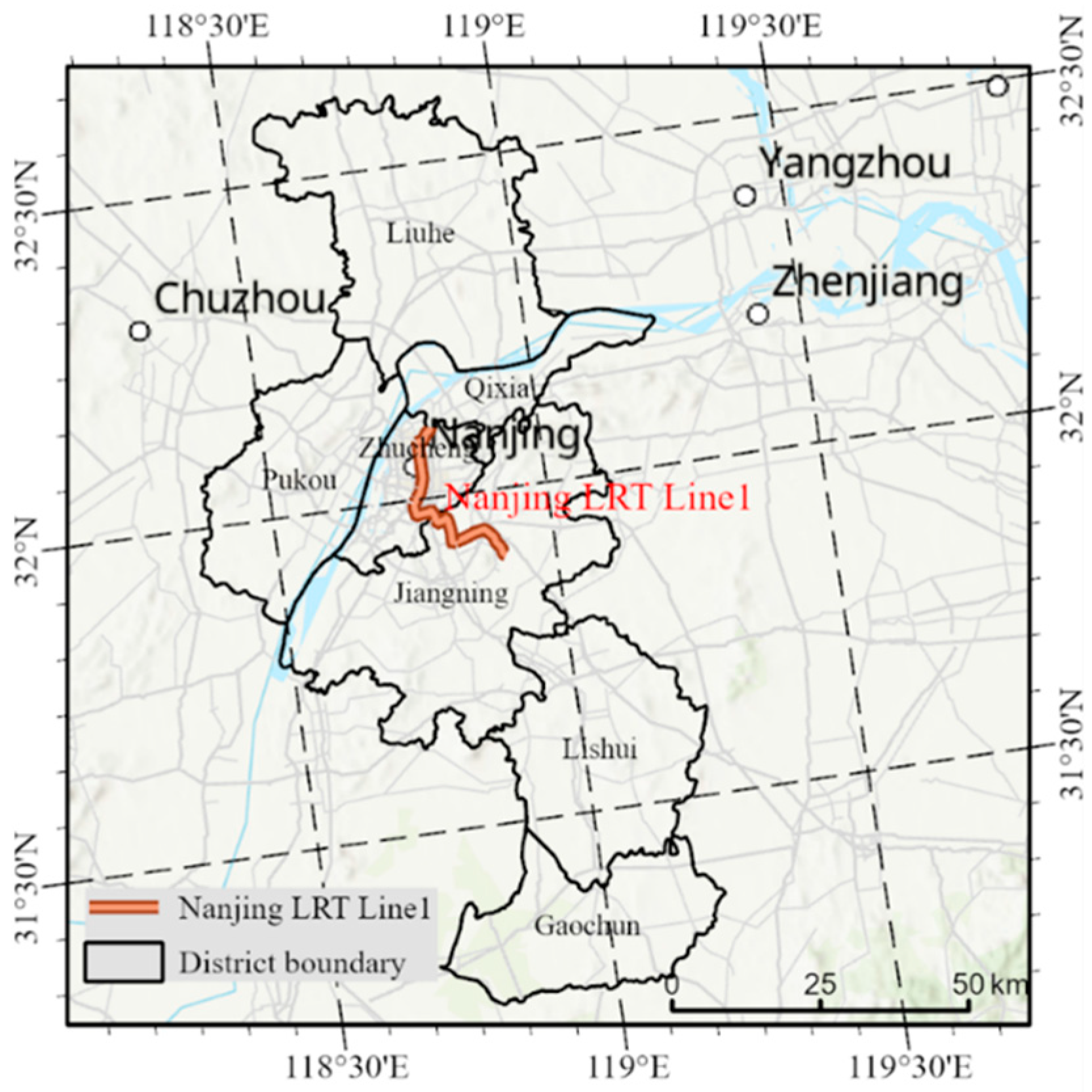
2. Study Area and Materials
3. Methodology
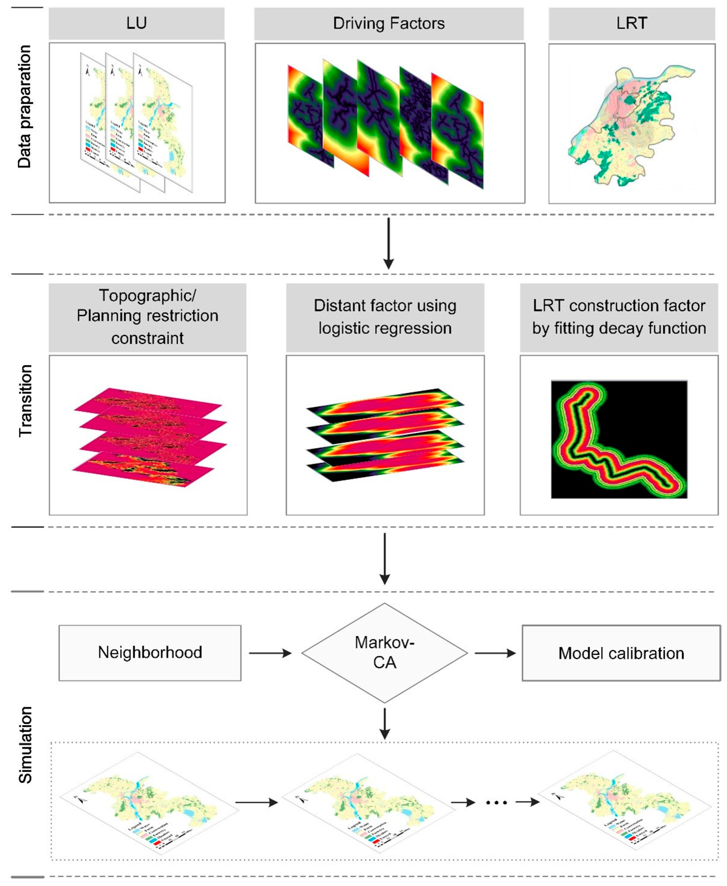
3.1. Basic Ideas of the Proposed CA Model
3.2. Transition Potential (T) and Constraint (Con) Establishment
3.2.1. Topographic Constraint ()
3.2.2. Planning Restriction Constraint ()
3.2.3. Distance Factor ()
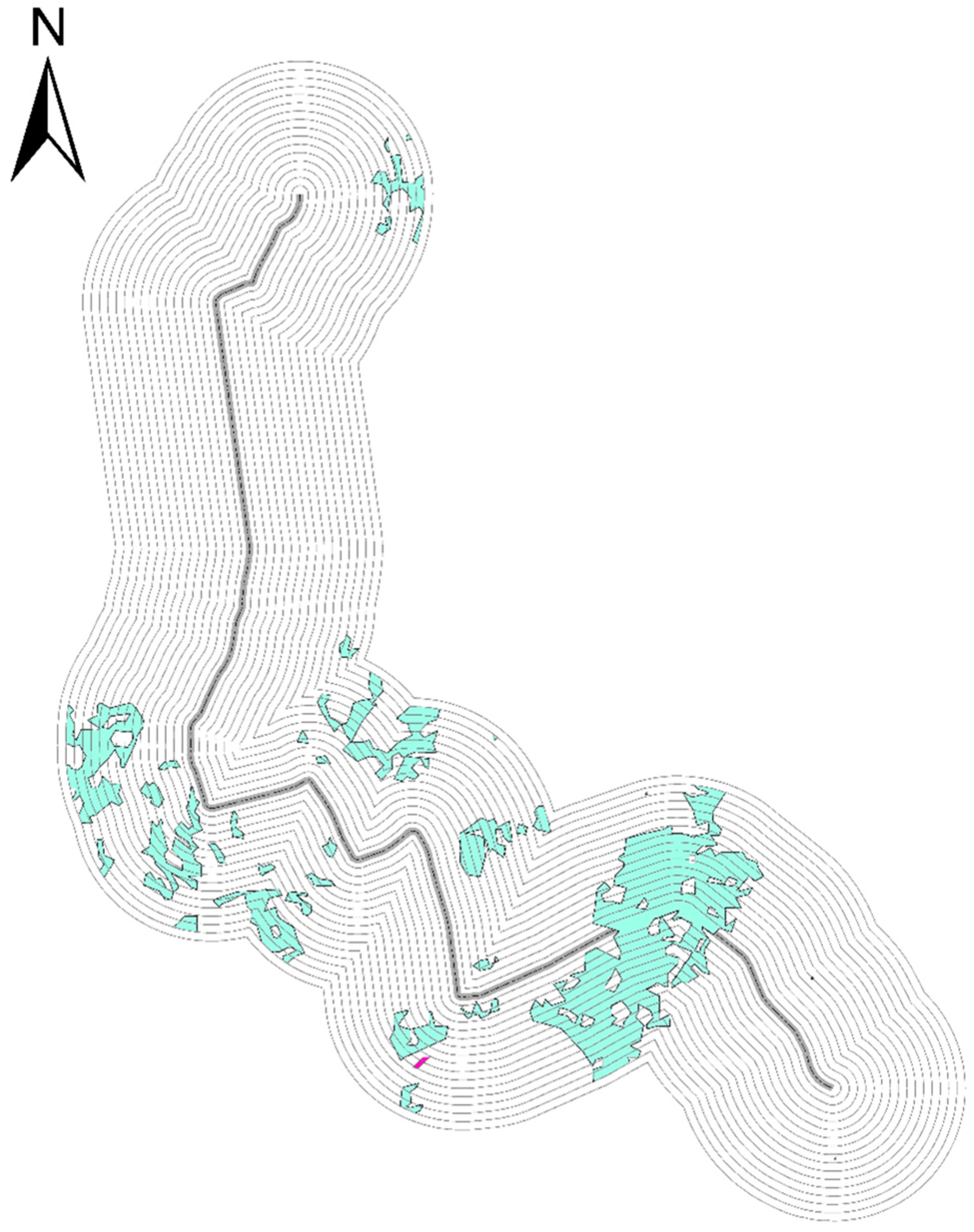
3.2.4. LRT Construction Factor ()
3.2.5. Final Transition Probability
3.3. Other Model Parameter Setting
3.3.1. Neighborhood (N)
3.3.2. Transition Possibility Threshold ()
3.3.3. Iteration Ending Condition
3.4. Model Performance Assessment
4. Results and Discussions
4.1. CA Transition Rule Result
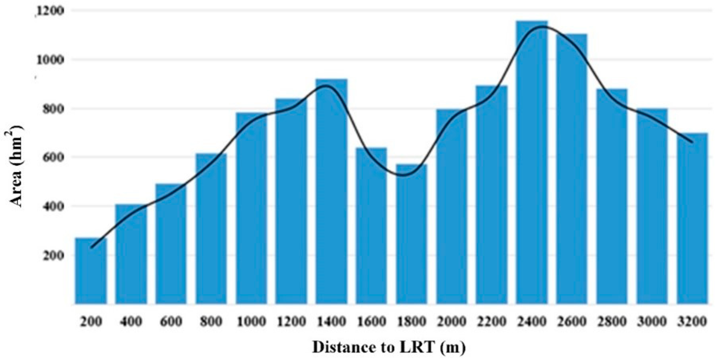
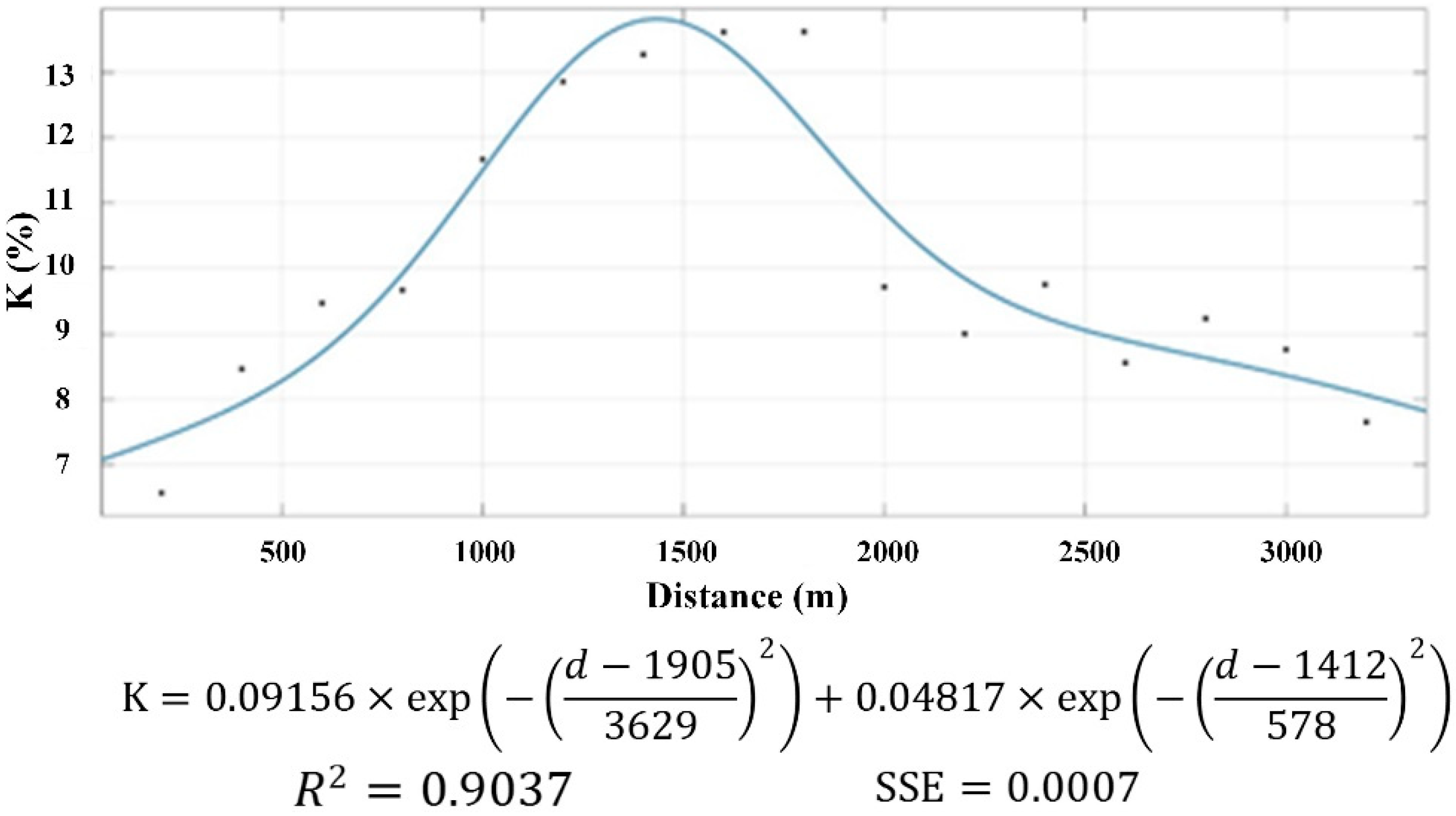
4.1.1. Distance Factor
4.1.2. LRT Factor
4.2. Model Parameter Result
4.2.1. Transition Possibility Threshold Result
4.2.2. Iteration Ending Condition Result by Markov Chain
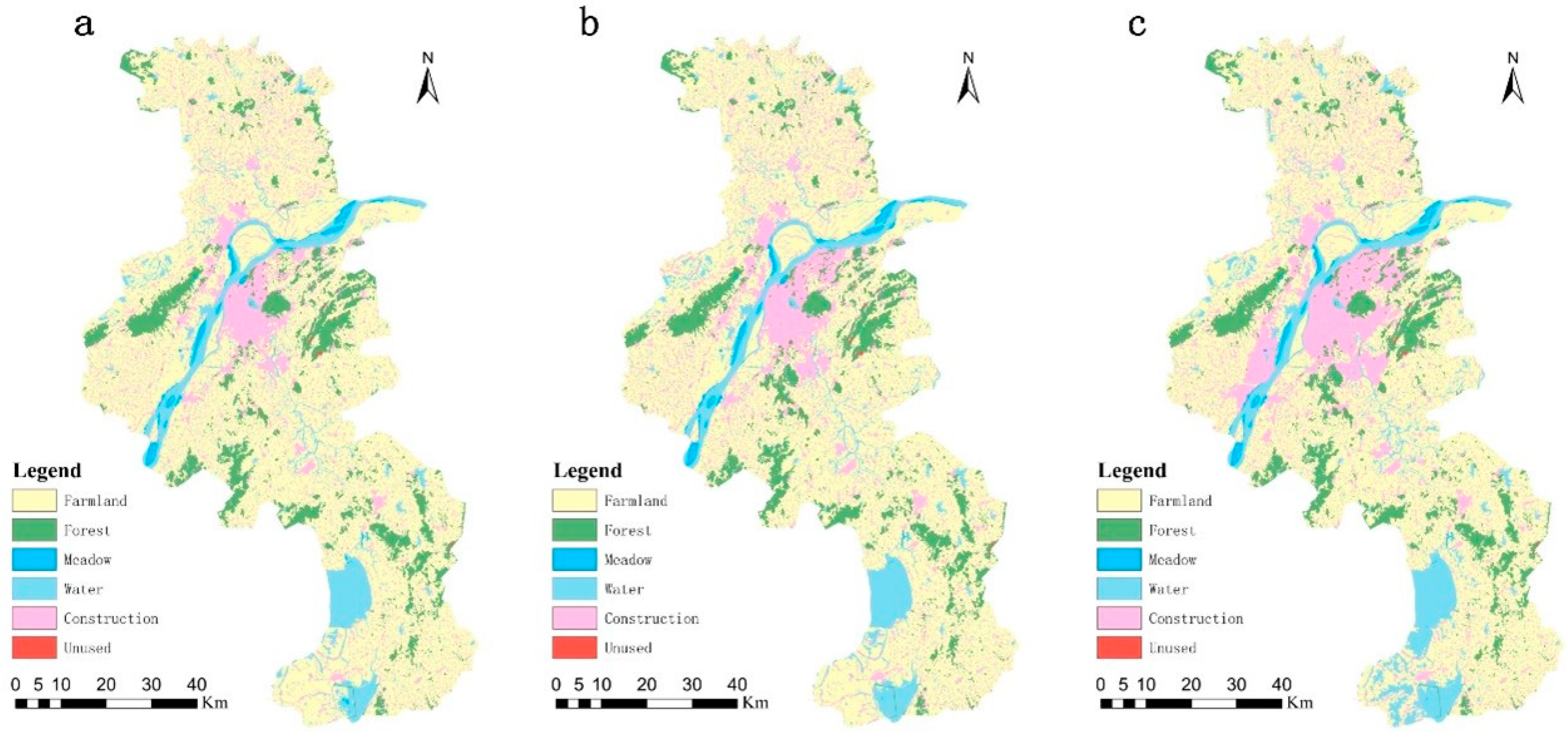
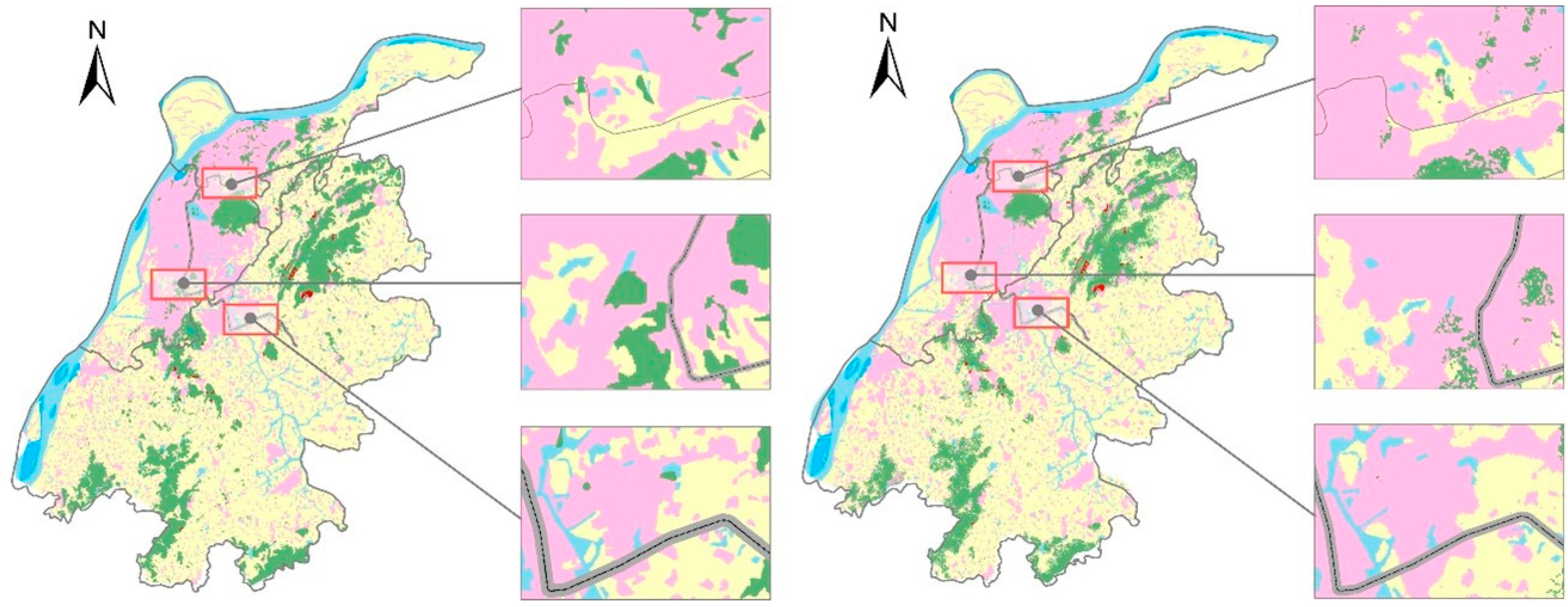
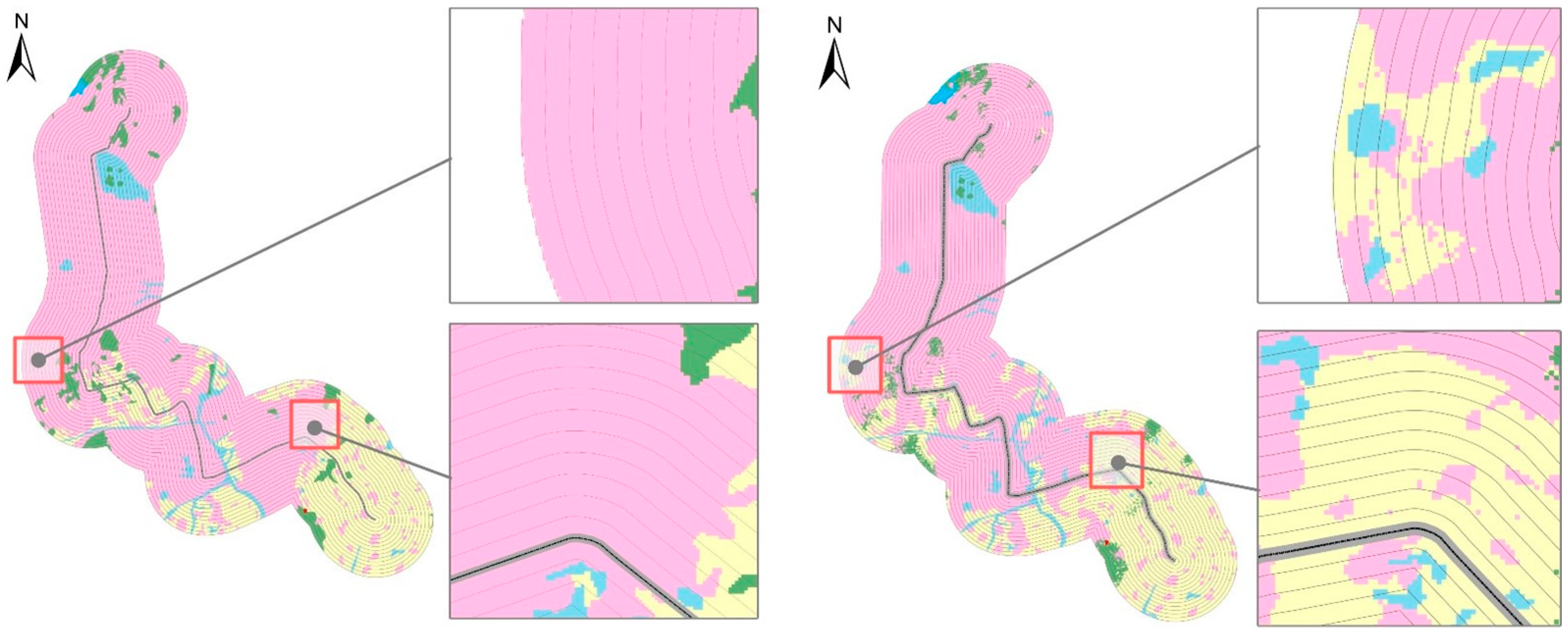
4.3. LUC Simulation Results
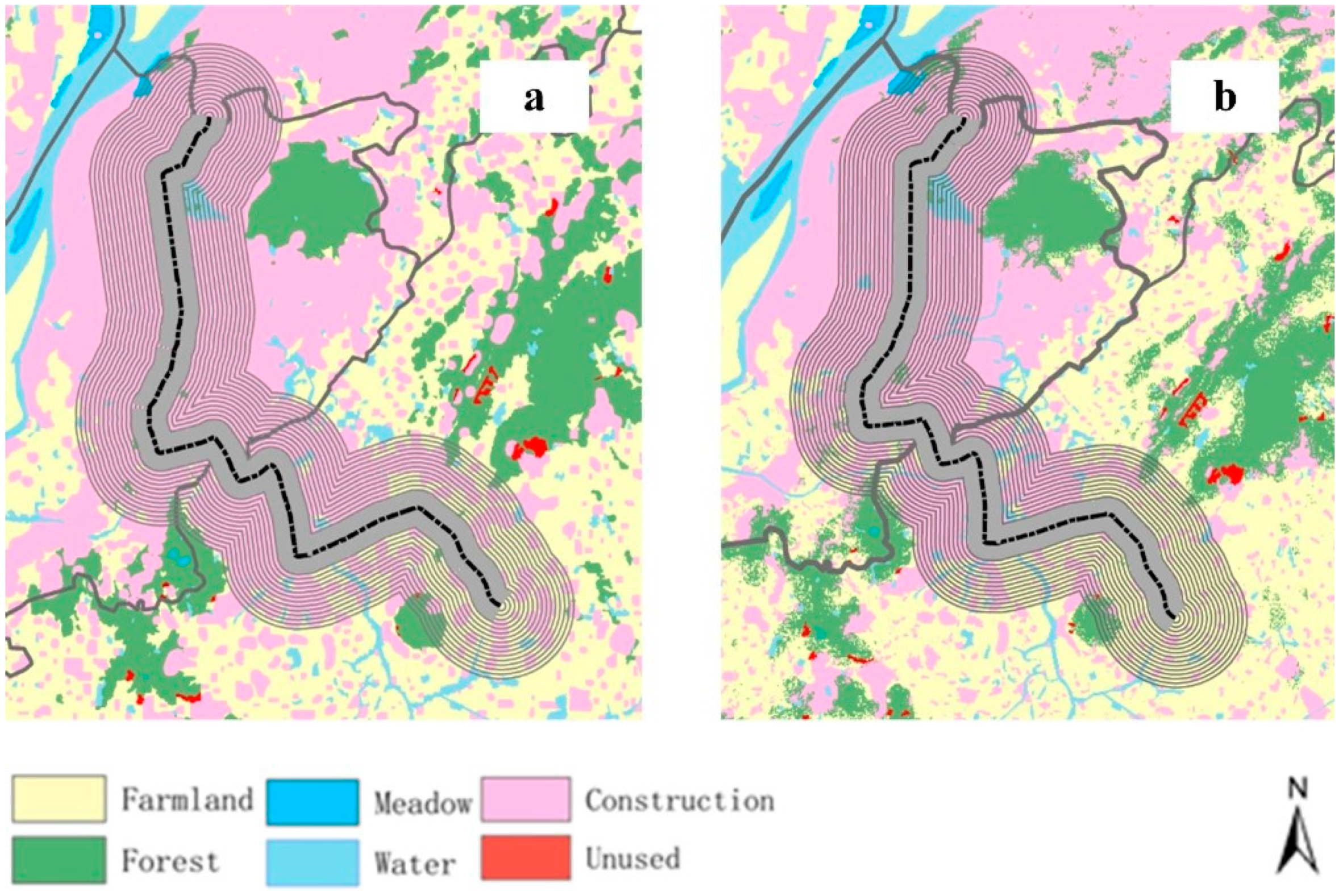
4.4. Comparison of CA Simulation between with/without Considering LRT Influence Factor
4.5. Comparison of CA Simulation between with/without Considering Spatiotemporal Heterogeneity of LRT Influence
5. Conclusions
Author Contributions
Funding
Data Availability Statement
Acknowledgments
Conflicts of Interest
References
- Clarke, K.C.; Hoppen, S.; Gaydos, L. A self-modifying cellular automaton model of historical urbanization in the San Francisco Bay area. Environ. Plan. B Plan. Des. 1997, 24, 247–261. [Google Scholar] [CrossRef] [Green Version]
- Verburg, P.H.; de Nijs, T.C.; van Eck, J.R.; Visser, H.; de Jong, K. A method to analyse neighbourhood characteristics of land use patterns. Comput. Environ. Urban Syst. 2004, 28, 667–690. [Google Scholar] [CrossRef]
- Seto, K.C.; Fragkias, M.; Güneralp, B.; Reilly, M.K. A meta-analysis of global urban land expansion. PLoS ONE 2011, 6, e23777. [Google Scholar] [CrossRef] [PubMed]
- Liu, X.; Liang, X.; Li, X.; Xu, X.; Ou, J.; Chen, Y.; Li, S.; Wang, S.; Pei, F. A future land use simulation model (FLUS) for simulating multiple land use scenarios by coupling human and natural effects. Landsc. Urban Plan. 2017, 168, 94–116. [Google Scholar] [CrossRef]
- Wu, F. Calibration of stochastic cellular automata: The application to rural-urban land conversions. Int. J. Geogr. Inf. Sci. 2002, 16, 795–818. [Google Scholar] [CrossRef]
- Pontius, R.G.; Boersma, W.; Castella, J.-C.; Clarke, K.; de Nijs, T.; Dietzel, C.; Duan, Z.; Fotsing, E.; Goldstein, N.; Kok, K. Comparing the input, output, and validation maps for several models of land change. Ann. Reg. Sci. 2008, 42, 11–37. [Google Scholar] [CrossRef] [Green Version]
- Liu, Y. Modelling sustainable urban growth in a rapidly urbanising region using a fuzzy-constrained cellular automata approach. Int. J. Geogr. Inf. Sci. 2012, 26, 151–167. [Google Scholar] [CrossRef]
- Rafiee, R.; Mahiny, A.S.; Khorasani, N.; Darvishsefat, A.A.; Danekar, A. Simulating urban growth in Mashad City, Iran through the SLEUTH model (UGM). Cities 2009, 26, 19–26. [Google Scholar] [CrossRef]
- Feng, Y. Modeling dynamic urban land-use change with geographical cellular automata and generalized pattern search-optimized rules. Int. J. Geogr. Inf. Sci. 2017, 31, 1198–1219. [Google Scholar]
- Zhu, J.; Sun, Y.; Song, S.; Yang, J.; Ding, H. Cellular automata for simulating land-use change with a constrained irregular space representation: A case study in Nanjing city, China. Environ. Plan. B Urban Anal. City Sci. 2020. [Google Scholar] [CrossRef]
- National Bureau of Statistics of China. Communiqué of the National Bureau of Statistics of People’s Republic of China on Major Figures of the 2010 Population Census; National Bureau of Statistics of China: Beijing, China, 2011.
- Cervero, R.; Dai, D. BRT TOD: Leveraging transit oriented development with bus rapid transit investments. Transp. Policy 2014, 36, 127–138. [Google Scholar] [CrossRef]
- Yang, P.; Wei, C. Metro-city planning practice: Wuhan example (in Chinese). Planners 2016, 32, 5–10. [Google Scholar]
- Wang, X.-F.; Xu, J.-G.; Li, Y.-F. Potential influences of rail transportation construction to land use differentiation in Nanjing. Hum. Geogr 2005, 20, 112–116. [Google Scholar]
- Zhang, M.; Wang, L. The impacts of mass transit on land development in China: The case of Beijing. Res. Transp. Econ. 2013, 40, 124–133. [Google Scholar] [CrossRef]
- Thapa, R.B.; Murayama, Y. Drivers of urban growth in the Kathmandu valley, Nepal: Examining the efficacy of the analytic hierarchy process. Appl. Geogr. 2010, 30, 70–83. [Google Scholar] [CrossRef]
- Duranton, G.; Turner, M.A. Urban growth and transportation. Rev. Econ. Stud. 2012, 79, 1407–1440. [Google Scholar] [CrossRef]
- Joshi, H.; Guhathakurta, S.; Konjevod, G.; Crittenden, J.; Li, K. Simulating the effect of light rail on urban growth in Phoenix: An application of the UrbanSim modeling environment. J. Urban Technol. 2006, 13, 91–111. [Google Scholar] [CrossRef]
- Pacheco-Raguz, J.F. Assessing the impacts of Light Rail Transit on urban land in Manila. J. Transp. Land Use 2010, 3, 113–138. [Google Scholar] [CrossRef] [Green Version]
- Bardaka, E.; Delgado, M.S.; Florax, R.J. Causal identification of transit-induced gentrification and spatial spillover effects: The case of the Denver light rail. J. Transp. Geogr. 2018, 71, 15–31. [Google Scholar] [CrossRef]
- Wang, J.; Feng, Y.; Ye, Z.; Tong, X.; Wang, R.; Gao, C.; Chen, S.; Lei, Z.; Liu, S.; Jin, Y. Simulating the effect of urban light rail transit on urban development by coupling cellular automata and conjugate gradients. Geocarto Int. 2020, 1–19. [Google Scholar] [CrossRef]
- Ratner, K.A.; Goetz, A.R. The reshaping of land use and urban form in Denver through transit-oriented development. Cities 2013, 30, 31–46. [Google Scholar] [CrossRef]
- Calvo, F.; de Oña, J.; Arán, F. Impact of the Madrid subway on population settlement and land use. Land Use Policy 2013, 31, 627–639. [Google Scholar] [CrossRef]
- Mokadi, E.; Mitsova, D.; Wang, X. Projecting the impacts of a proposed streetcar system on the urban core land redevelopment: The case of Cincinnati, Ohio. Cities 2013, 35, 136–146. [Google Scholar] [CrossRef]
- Comber, S.; Arribas-Bel, D. “Waiting on the train”: The anticipatory (causal) effects of Crossrail in Ealing. J. Transp. Geogr. 2017, 64, 13–22. [Google Scholar] [CrossRef] [Green Version]
- Pan, H.; Zhang, M. Rail transit impacts on land use: Evidence from Shanghai, China. Transp. Res. Rec. 2008, 2048, 16–25. [Google Scholar] [CrossRef]
- Bhattacharjee, S.; Goetz, A.R. The rail transit system and land use change in the Denver metro region. J. Transp. Geogr. 2016, 54, 440–450. [Google Scholar] [CrossRef]
- Ahmad, S.; Avtar, R.; Sethi, M.; Surjan, A. Delhi’s land cover change in post transit era. Cities 2016, 50, 111–118. [Google Scholar] [CrossRef]
- Iacono, M.J.; Levinson, D.M. Predicting land use change: How much does transportation matter? Transp. Res. Rec. 2009, 2119, 130–136. [Google Scholar] [CrossRef] [Green Version]
- Hurst, N.B.; West, S.E. Public transit and urban redevelopment: The effect of light rail transit on land use in Minneapolis, Minnesota. Reg. Sci. Urban Econ. 2014, 46, 57–72. [Google Scholar] [CrossRef]
- Golub, A.; Guhathakurta, S.; Sollapuram, B. Spatial and temporal capitalization effects of light rail in Phoenix: From conception, planning, and construction to operation. J. Plan. Educ. Res. 2012, 32, 415–429. [Google Scholar] [CrossRef]
- Cervero, R. Linking urban transport and land use in developing countries. J. Transp. Land Use 2013, 6, 7–24. [Google Scholar] [CrossRef] [Green Version]
- Tan, Z.; Li, S.; Li, X.; Liu, X.; Chen, Y.; Li, W. Spatio-temporal effects of urban rail transit on complex land-use change. Acta Geogr. Sinica 2017, 72, 850–862. [Google Scholar]
- Li, S.; Liu, X.; Li, Z.; Wu, Z.; Yan, Z.; Chen, Y.; Gao, F. Spatial and temporal dynamics of urban expansion along the Guangzhou–Foshan inter-city rail transit corridor, China. Sustainability 2018, 10, 593. [Google Scholar] [CrossRef] [Green Version]
- Zhang, H.; Li, X.; Liu, X.; Chen, Y.; Ou, J.; Niu, N.; Jin, Y.; Shi, H. Will the Development of a High-Speed Railway Have Impacts on Land Use Patterns in China? Ann. Am. Assoc. Geogr. 2019, 109, 979–1005. [Google Scholar] [CrossRef]
- Rodriguez, D.A.; Vergel-Tovar, E.; Camargo, W.F. Land development impacts of BRT in a sample of stops in Quito and Bogotá. Transp. Policy 2016, 51, 4–14. [Google Scholar] [CrossRef]
- Aljoufie, M.; Brussel, M.; Zuidgeest, M.; van Delden, H.; van Maarseveen, M. Integrated analysis of land-use and transport policy interventions. Transp. Plan. Technol. 2016, 39, 329–357. [Google Scholar] [CrossRef]
- Lin, J.; Chen, T.; Han, Q. Simulating and predicting the impacts of light rail transit systems on urban land use by using cellular automata: A case study of Dongguan, China. Sustainability 2018, 10, 1293. [Google Scholar] [CrossRef] [Green Version]
- Zhao, L.; Shen, L. The impacts of rail transit on future urban land use development: A case study in Wuhan, China. Transp. Policy 2019, 81, 396–405. [Google Scholar] [CrossRef]
- Yang, J.; Shi, F.; Sun, Y.; Zhu, J. A cellular automata model constrained by spatiotemporal heterogeneity of the urban development strategy for simulating land-use change: A case study in Nanjing City, China. Sustainability 2019, 11, 4012. [Google Scholar] [CrossRef] [Green Version]
- Li, X.; Yang, Q.; Liu, X. Discovering and evaluating urban signatures for simulating compact development using cellular automata. Landsc. Urban Plan. 2008, 86, 177–186. [Google Scholar] [CrossRef]
- Li, X.; Lin, J.; Chen, Y.; Liu, X.; Ai, B. Calibrating cellular automata based on landscape metrics by using genetic algorithms. Int. J. Geogr. Inf. Sci. 2013, 27, 594–613. [Google Scholar] [CrossRef]
- Ayazli, I.E.; Kilic, F.; Lauf, S.; Demir, H.; Kleinschmit, B. Simulating urban growth driven by transportation networks: A case study of the Istanbul third bridge. Land Use Policy 2015, 49, 332–340. [Google Scholar] [CrossRef]
- Willigers, J.; Van Wee, B. High-speed rail and office location choices. A stated choice experiment for the Netherlands. J. Transp. Geogr. 2011, 19, 745–754. [Google Scholar] [CrossRef]
- Murakami, J.; Cervero, R. High-Speed Rail and Economic Development: Business Agglomerations and Policy Implications; University of California Transportation Center: Berkeley, CA, USA, 2012. [Google Scholar]
- Garmendia, M.; Romero, V.; Ureña, J.M.D.; Coronado, J.M.; Vickerman, R. High-speed rail opportunities around metropolitan regions: Madrid and London. J. Infrastruct. Syst. 2012, 18, 305–313. [Google Scholar] [CrossRef]
- Cao, M.; Bennett, S.J.; Shen, Q.; Xu, R. A bat-inspired approach to define transition rules for a cellular automaton model used to simulate urban expansion. Int. J. Geogr. Inf. Sci. 2016, 30, 1961–1979. [Google Scholar] [CrossRef]
- Luo, J.; Wei, Y.D. Modeling spatial variations of urban growth patterns in Chinese cities: The case of Nanjing. Landsc. Urban Plan. 2009, 91, 51–64. [Google Scholar] [CrossRef]
- Shu, B.; Bakker, M.M.; Zhang, H.; Li, Y.; Qin, W.; Carsjens, G.J. Modeling urban expansion by using variable weights logistic cellular automata: A case study of Nanjing, China. Int. J. Geogr. Inf. Sci. 2017, 31, 1314–1333. [Google Scholar] [CrossRef]
- Omrani, H.; Tayyebi, A.; Pijanowski, B. Integrating the multi-label land-use concept and cellular automata with the artificial neural network-based land transformation model: An integrated ML-CA-LTM modeling framework. GIScience Remote Sens. 2017, 54, 283–304. [Google Scholar] [CrossRef] [Green Version]
- Guerra, E.; Cervero, R.; Tischler, D. Half-mile circle: Does it best represent transit station catchments? Transp. Res. Rec. 2012, 2276, 101–109. [Google Scholar] [CrossRef] [Green Version]
- Cao, X.J.; Porter-Nelson, D. Real estate development in anticipation of the Green Line light rail transit in St. Paul. Transp. Policy 2016, 51, 24–32. [Google Scholar] [CrossRef] [Green Version]
- Kwoka, G.J.; Boschmann, E.E.; Goetz, A.R. The impact of transit station areas on the travel behaviors of workers in Denver, Colorado. Transp. Res. Part A Policy Pract. 2015, 80, 277–287. [Google Scholar] [CrossRef]
- Barreira-González, P.; Gómez-Delgado, M.; Aguilera-Benavente, F. From raster to vector cellular automata models: A new approach to simulate urban growth with the help of graph theory. Comput. Environ. Urban Syst. 2015, 54, 119–131. [Google Scholar] [CrossRef]
- Wu, H.; Zhou, L.; Chi, X.; Li, Y.; Sun, Y. Quantifying and analyzing neighborhood configuration characteristics to cellular automata for land use simulation considering data source error. Earth Sci. Inform. 2012, 5, 77–86. [Google Scholar] [CrossRef]
- Feng, Y.; Tong, X. Incorporation of spatial heterogeneity-weighted neighborhood into cellular automata for dynamic urban growth simulation. GIScience Remote Sens. 2019, 56, 1024–1045. [Google Scholar] [CrossRef]
- Jing, L. Research on the Urban Land-Use along the High-Capacity Rail Rapid Transit Line—A Case Study of Wuhan No. 2 Rail Transit Line. Ph.D. Thesis, Huazhong University of Science of Technology, Wuhan, China, 2005. [Google Scholar]
- Todes, A. Urban growth and strategic spatial planning in Johannesburg, South Africa. Cities 2012, 29, 158–165. [Google Scholar] [CrossRef]


| Spatial Variables | Data Source | Calculation Method | |
|---|---|---|---|
| Topographic constraint | Slope | DEM | Slope tool in ArcGIS |
| Planning Restriction constraint | Farmland protection | Master plan | Extract and reclassify |
| Habitat Conservation | |||
| Distance Factor | Distance to water () | LU | Euclidean distance function |
| Distance to railway () | Road network | ||
| Distance to highway () | |||
| Distance to national highway () | |||
| Distance to provincial road () | |||
| Distance to county road () | |||
| Distance to municipal center () | Master plan | ||
| Distance to county center () | |||
| LRT Construction Factor | LRT | Road network | Euclidean distance function and Gauss decay function |
| Coefficient/LU | Farmland | Forest | Meadow | Water | Construction |
|---|---|---|---|---|---|
| 0.63 | 0.33 | −1.35 | - | 0.65 | |
| −0.20 | −0.36 | 3.55 | −0.12 | - | |
| −2.40 | - | 2.25 | 2.43 | 1.25 | |
| 1.50 | −1.82 | −1.96 | −1.52 | −0.72 | |
| - | −1.05 | 1.56 | 0.67 | 0.85 | |
| −1.52 | −0.86 | 2.52 | 3.23 | −1.85 | |
| 0.55 | 0.55 | −5.35 | −0.23 | −0.45 |
| Construction | Unused | Forest | Water | Farmland | Meadow | |
|---|---|---|---|---|---|---|
| Construction | 407.94 | 0.15 | 0.59 | 26.26 | 51.32 | 0.12 |
| Unused | 0.68 | 1.33 | 0.28 | 0.00 | 0.00 | 0.02 |
| Forest | 40.23 | 0.02 | 231.09 | 0.11 | 2.01 | 0.03 |
| Water | 26.28 | 0.00 | 0.86 | 237.84 | 17.90 | 0.00 |
| Farmland | 195.82 | 0.09 | 1.48 | 118.55 | 1226.02 | 1.28 |
| Meadow | 0.00 | 0.03 | 2.14 | 1.54 | 0.03 | 20.34 |
| Districts /LU | Water | Farmland | Construction | Unused | Meadow | Forestry |
|---|---|---|---|---|---|---|
| Qixia | 0.186 | 0.212 | 0.251 | 0.225 | 0.214 | 0.216 |
| Pukou | 0.197 | 0.225 | 0.221 | 0.169 | 0.211 | 0.214 |
| Zhucheng | 0.206 | 0.211 | 0.276 | 0.178 | 0.185 | 0.219 |
| Jiangning | 0.215 | 0.212 | 0.245 | 0.203 | 0.224 | 0.213 |
| Liuhe | 0.212 | 0.222 | 0.223 | 0.210 | 0.219 | 0.221 |
| Lishui | 0.222 | 0.215 | 0.192 | 0.218 | 0.231 | 0.211 |
| Gaochun | 0.216 | 0.214 | 0.208 | 0.221 | 0.216 | 0.221 |
| Qixia | Jiangning | Zhucheng | Pukou | Liuhe | Lishui | Gaochun | |
|---|---|---|---|---|---|---|---|
| LRT impact | 0.251 | 0.245 | 0.276 | 0.221 | 0.223 | 0.192 | 0.208 |
| NO LRT | 0.190 | 0.186 | 0.174 | 0.221 | 0.223 | 0.192 | 0.208 |
| Distance (m) | Relative Error | Distance (m) | Relative Error | ||
|---|---|---|---|---|---|
| Ours | Linear | Ours | Linear | ||
| 0–200 | 1.74% | 5.11% | 1600–1800 | 7.69% | 18.74% |
| 200–400 | 1.78% | 4.31% | 1800–2000 | 5.25% | 22.66% |
| 400–600 | 1.23% | 8.09% | 2000–2200 | 4.67% | 23.24% |
| 600–800 | 0.37% | 14.30% | 2200–2400 | 3.89% | 22.78% |
| 800–1000 | 6.83% | 12.64% | 2400–2600 | 0.81% | 26.08% |
| 1000–1200 | 8.38% | 7.03% | 2600–2800 | 2.99% | 21.23% |
| 1200–1400 | 9.79% | 6.16% | 2800–3000 | 5.21% | 11.55% |
| 1400–1600 | 8.16% | 11.68% | 3000–3200 | 5.32% | 10.23% |
Publisher’s Note: MDPI stays neutral with regard to jurisdictional claims in published maps and institutional affiliations. |
© 2021 by the authors. Licensee MDPI, Basel, Switzerland. This article is an open access article distributed under the terms and conditions of the Creative Commons Attribution (CC BY) license (https://creativecommons.org/licenses/by/4.0/).
Share and Cite
Na, J.; Zhu, J.; Zheng, J.; Di, S.; Ding, H.; Ma, L. Cellular Automata Based Land-Use Change Simulation Considering Spatio-Temporal Influence Heterogeneity of Light Rail Transit Construction: A Case in Nanjing, China. ISPRS Int. J. Geo-Inf. 2021, 10, 308. https://0-doi-org.brum.beds.ac.uk/10.3390/ijgi10050308
Na J, Zhu J, Zheng J, Di S, Ding H, Ma L. Cellular Automata Based Land-Use Change Simulation Considering Spatio-Temporal Influence Heterogeneity of Light Rail Transit Construction: A Case in Nanjing, China. ISPRS International Journal of Geo-Information. 2021; 10(5):308. https://0-doi-org.brum.beds.ac.uk/10.3390/ijgi10050308
Chicago/Turabian StyleNa, Jiaming, Jie Zhu, Jiazhu Zheng, Shaoning Di, Hu Ding, and Lingfei Ma. 2021. "Cellular Automata Based Land-Use Change Simulation Considering Spatio-Temporal Influence Heterogeneity of Light Rail Transit Construction: A Case in Nanjing, China" ISPRS International Journal of Geo-Information 10, no. 5: 308. https://0-doi-org.brum.beds.ac.uk/10.3390/ijgi10050308