Detection and Analysis of Degree of Maize Lodging Using UAV-RGB Image Multi-Feature Factors and Various Classification Methods

Abstract

Maize (Zea mays L.), one of the most important agricultural crops in the world, which can be devastated by lodging, which can strike maize during its growing season. Maize lodging affects not only the yield but also the quality of its kernels. The identification of lodging is helpful to evaluate losses due to natural disasters, to screen lodging-resistant crop varieties, and to optimize field-management strategies. The accurate detection of crop lodging is inseparable from the accurate determination of the degree of lodging, which helps improve field management in the crop-production process. An approach was developed that fuses supervised and object-oriented classifications on spectrum, texture, and canopy structure data to determine the degree of lodging with high precision. The results showed that, combined with the original image, the change of the digital surface model, and texture features, the overall accuracy of the object-oriented classification method using random forest classifier was the best, which was 86.96% (kappa coefficient was 0.79). The best pixel-level supervised classification of the degree of maize lodging was 78.26% (kappa coefficient was 0.6). Based on the spatial distribution of degree of lodging as a function of crop variety, sowing date, densities, and different nitrogen treatments, this work determines how feature factors affect the degree of lodging. These results allow us to rapidly determine the degree of lodging of field maize, determine the optimal sowing date, optimal density and optimal fertilization method in field production.

1. Introduction

Maize (Zea mays L.) is the most planted crop in the world and plays an important role in ensuring China’s national food security [1]. Lodging, which can devastate maize crops at any time in the growing season, mostly occurs from the tasseling stage to the filling stage [2]. The relentless pursuit of yield of modern agriculture leads to vigorous growth of maize and dense planting, which makes for long, thin maize stalks that can easily fall victim to maize lodging through heavy storms and rains in occurring in China mainly during the growth stages from tasseling to filling [2]. Maize lodging causes mechanical damage to the maize stalk and leads to various degrees of bending, which reduces nutrient absorption and transport, affects the synthesis of organic matter and the normal development of maize, and ultimately destroys the canopy structure, thereby decimating the grain yield and quality [3]. It is thus vital to obtain timely and accurate information on maize lodging after such disasters not only to help agricultural production authorities take remedial measures quickly and reduce losses but also to help insurance companies estimate losses quickly and accurately and thereby provide reasonable compensation after such disasters. In addition, such an approach would allow us to select lodging-resistant crop varieties and improve field-management strategies.

Obtaining data on the maize lodging through ground investigation and actual measurement is time-consuming and inefficient. However, the recent development of remote-sensing technology now offers a convenient way to rapidly obtain crop-lodging data [4,5]. Recent years have seen the development of remote-sensing technology based on unmanned aerial vehicles (UAVs), which are able to capture RGB images with higher spatial and temporal resolution than is possible with satellite remote-sensing technology [6]. In addition, UAVs offer high scalability and can carry a variety of optical sensors, all with lower operating costs and complexity than was previously possible [7]. As a result, UAV remote sensing is gaining in popularity for acquiring crop spectral and structural data [8].

When crops grow normally, canopy leaves play a major role in reflectance; however, once lodging occurs, the spectral information comes mainly from crop stems [9], so different degrees of lodging lead to different reflectance spectra. Because the separation between plants decreases as the degree of lodging increases, maize stems contribute more to canopy reflectance as the degree of lodging increases [10]. In a UAV remote-sensing experiment, Li et al. [8] obtained RGB images of maize lodging at the filling stage, selected color and texture features of normal and lodged maize, and then extracted data on the maize lodging area. The results show the most accurate classification is based on mean texture features (minimum error is 0.3%, maximum error is 6.9%). This method produces minimal experimental error, so the area extracted is classified relatively accurately, thereby providing a basis for estimating crop lodging based on UAV remote sensing. In previous work on this subject, Liu et al. [11] combined RGB and thermal infrared imaging to establish a comprehensive recognition model for the rice lodging based on particle swarm optimization and the SVM algorithm. Their model enhanced the temperature difference between lodging and non-lodging rice, which improves the accuracy of lodging identification. Han et al. [12] analyzed RGB and multispectral images to extract potential characteristic factors and thereby predict maize lodging. They also formed a nomogram, calculated the risk and protection factors related to maize lodging, and calculated the probability of the maize lodging given different prediction variables. The results show that the canopy structure is the main factor affecting maize lodging. Chu et al. [13] used a UAV system equipped with RGB and near-infrared cameras to obtain RGB images of maize at different growth stages, which, when combined with structure-from-motion technologies, served to construct a three-dimensional canopy structure and digital surface model (DSM), from which the change in elevation is obtained before and after lodging. Elevation estimates from this method are consistent with ground measurements. Sun et al. [14] combined texture features with the vegetation index to classify different feature images by maximum likelihood classification and extracted four degrees of lodging. The comprehensive accuracy of the method combining texture features with the vegetation index is 86.61%, with a kappa coefficient of 0.8327.

At present, detecting crop lodging based on remote sensing mainly uses the single-element features of a single sensor to obtain pixel-level supervised classification. Few studies are available on high-precision classification based on the combination of spectra, texture, canopy structure, and other information, and the classification results rarely provide the degree of lodging. For instance, Guo et al. [15] used UAVs RGB images to construct the vegetation indexes, which they combined with texture features to classify crops. Research shows that classification based on the vegetation index and texture is clearly superior to single-factor classification. Wang et al. [16] constructed a normalized vegetation index based on the UAV remote-sensing images in the visible range separated into red, green, and blue bands. With the appropriate threshold, they extracted healthy green vegetation with an accuracy of over 90%.

Precise detection of crop lodging is thought to be inseparable from an accurate description of degree of lodging, which is helpful for targeted field management in the later stages of maize growth. In addition, although the traditional pixel-based classification methods are suitable for low- and medium-resolution satellite remote-sensing images, confusion arises with high-resolution images [17]. To overcome this problem, object-oriented classification, also known as object-based image analysis (OBIA), was used for high-spatial-resolution remote-sensing imaging. This method divides the image into adjacent, homogeneous regions and then identifies ground objects through a comprehensive analysis of various image features (spectra, geometry, textures, and context) to improve classification accuracy. The method offers high precision and high efficiency, so it is currently receiving a large share of attention among the remote-sensing information-extraction methods [18]. However, with this approach, the noise generated by pixel-level supervised classification is difficult to eliminate via filtering algorithms, which seriously affects the accuracy of the image classification results. Given the shortcomings of previous research, one focus of the present research is to classify maize lodging grades and with better accuracy by combining multiple feature factors and object-oriented classification methods. A similar approach was used by Jing et al. [19], who extracted data on aquatic vegetation in constructed wetland by using the RGB vegetation index and object-oriented classification, improving the classification accuracy from 53.7% for the traditional method to 91.7%. The results show that the object-oriented classification method significantly reduces noise and improves the classification accuracy.

The present study integrates multiple feature factors into the image-object layer and uses object-oriented classification to classify experimental maize fields via different experimental processes. The goal is to reduce salt-and-pepper noise in the traditional pixel-level supervised classification method and thereby improve the classification. In addition, the factors that determine the degree of lodging are analyzed based on the high-precision classification from the various experimental processes. The research results are helpful for screening lodging-resistant varieties, determining the critical growth period for lodging, and improving the level of field management.

2. Materials and Methods

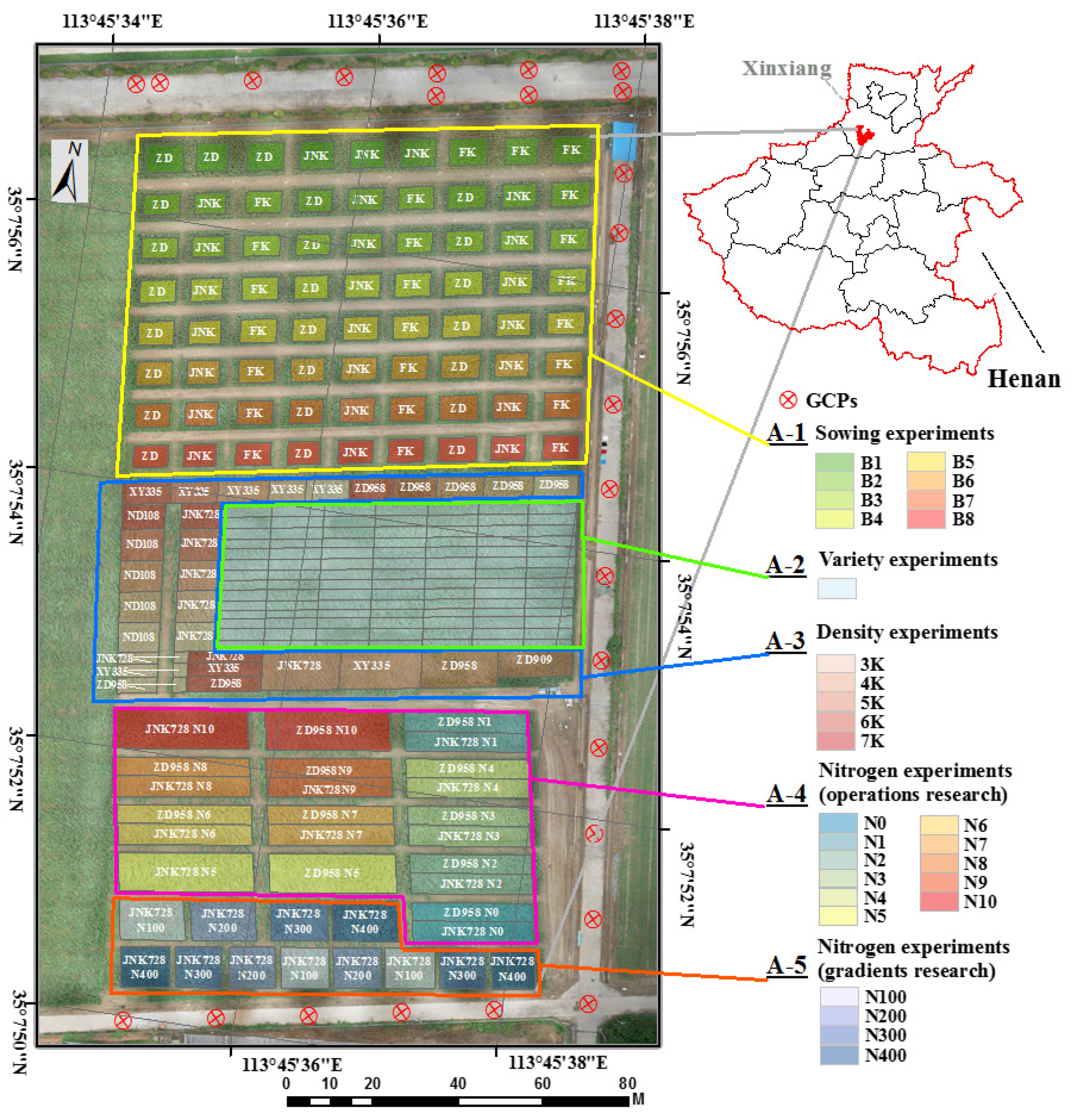
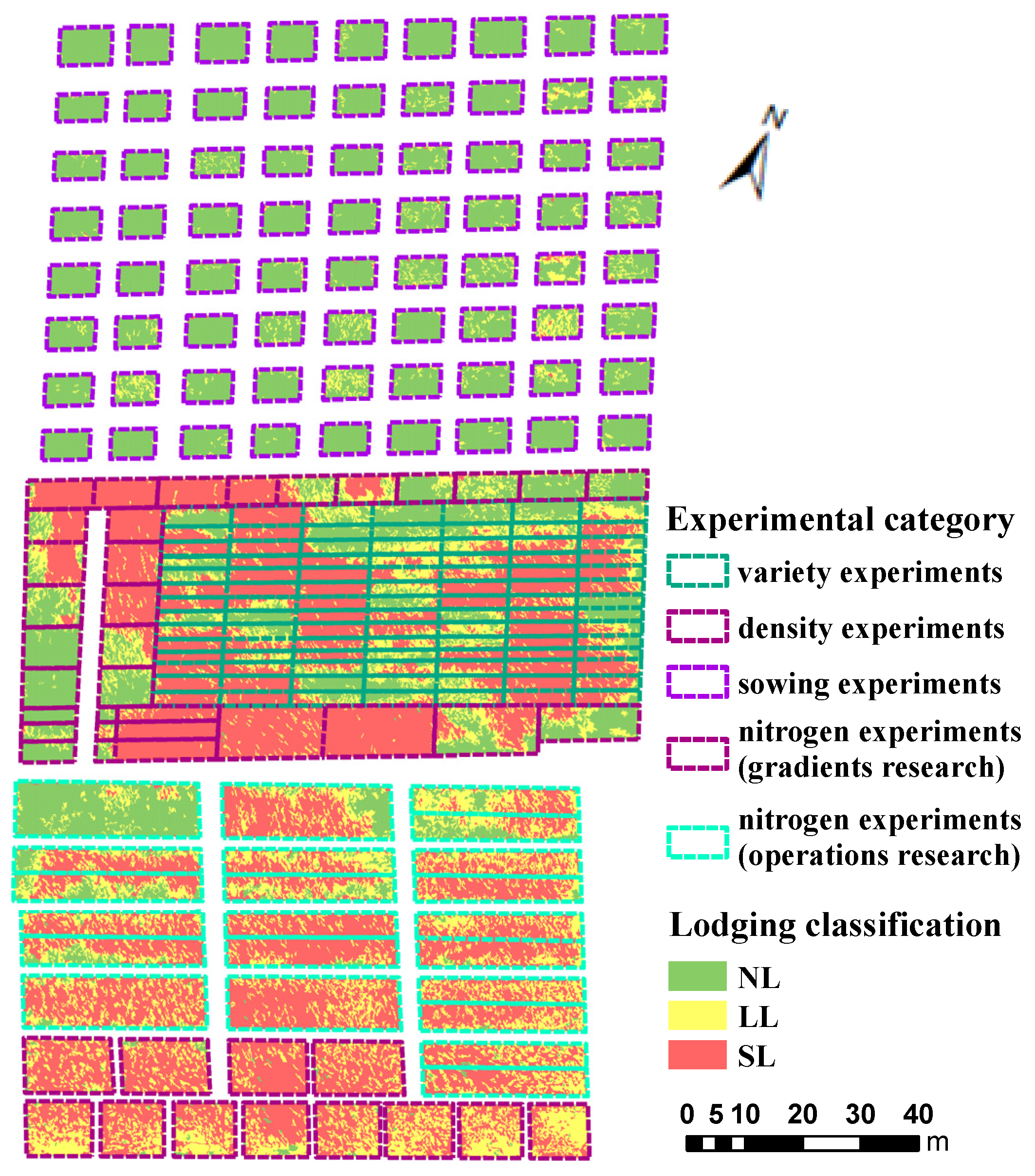
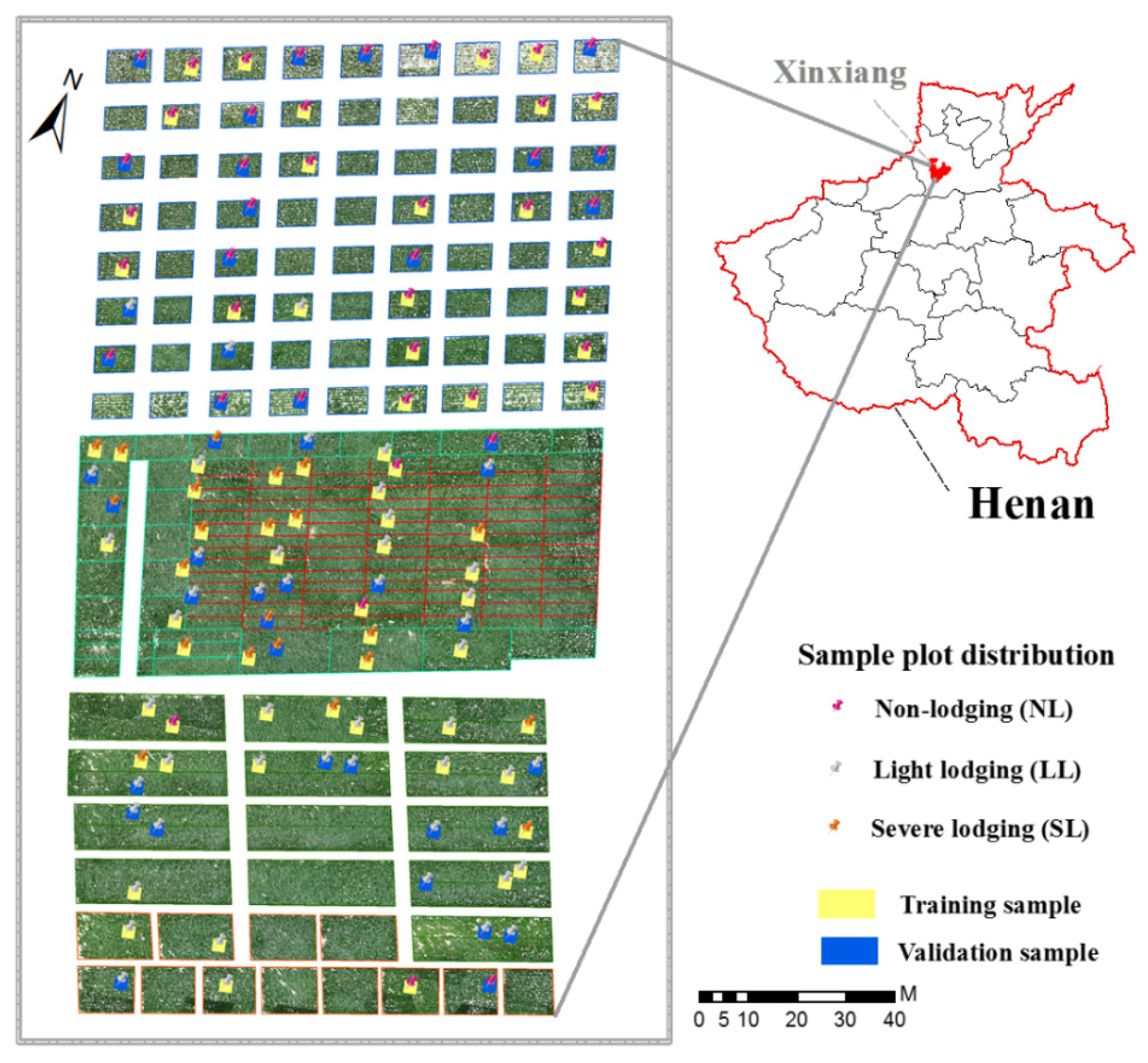
2.1. Study Area and Design of Field Experiments

The experimental site was in the southwest corner of the Xinxiang comprehensive experimental base of the Chinese Academy of Agricultural Sciences in the north of Henan Province (35°7′51.6″ N, 113°45′58″ E, altitude 75 m). Xinxiang County is west of the central part of the North China Plain and has a temperate continental monsoon climate, with four distinct seasons. The annual average temperature, the temperature difference, solar insolation potential, frost-free period, and precipitation are 14.3 °C, 16.5 °C, 2407 h, 191 days, and 560.6 mm, respectively. Seventy-five percent of the annual precipitation is concentrated between June and September.

The total planting area of summer maize was 3.43 ha, which was split into five experimental areas: sowing experiments (A-1), variety experiments (A-2), density experiments (A-3), nitrogen experiments (operations research) (A-4) and nitrogen experiments (gradients research) (A-5). The maize varieties FK139, JNK728, and ZD958, which are widely planted in North China, were used in the sowing experiments (A-1). The three varieties were planted at intervals, with the first sowing date to the eighth sowing date planted from north to south with passages between each plot, as shown in Figure 1. The first sowing was done on 24 April 2020, and the subsequent sowing was done at subsequent 10-day intervals. The sixth sowing date (24 June 2020) was the same as the sowing dates of the other experiments in areas A-2–A-5. For the variety experiments (A-2), 98 maize varieties were planted over an area of 3 m × 10 m with different genotypes and resistance to lodging. The A-3 density experiments were distributed on the west, north, and south sides of area A-2 (see Figure 1); on the north and west sides were planted the varieties XY335, ZD958, and ND108 at densities of 105,000, 90,000, 75,000, 60,000, and 45,000 ha⁻¹.The varieties JNK728, XY335, ZD958, and ZD909 were planted to the south of area A-2 at densities of 75,000, 75,000, and 105,000 ha⁻¹. Figure 1 shows the spatial distribution. For the density experiments, wide sowing was used. A planting density of 75,000 ha⁻¹ was used for experimental areas A-1, A-2, A-4, and A-5, with a row spacing of 60 cm and a plant spacing of 23 cm. To the south of the test field were the nitrogen operation and gradient experiments (A-4 and A-5). The operation experiment used maize varieties JNK728 and ZD958, with a total of 11 nitrogen application methods. Figure 1 shows the spatial distribution of nitrogen application modes. The gradient experiment used maize variety JNK728 and involved four nitrogen treatments denoted N100, N200, N300, and N400.Urea (CH₄N₂O) was used as nitrogen source. Figure 1 shows the spatial distribution of nitrogen application modes in area A-5. For the nitrogen treatment, urea (CH₄N₂O), superphosphate (P₂O₅), and potassium oxide (K₂O) were mixed into the soil before the experimental sowing date for areas A-1, A-2, and A-3, and the base fertilizer was applied a single time as per the normal local field management.

Table 1. Nitrogen treatment application methods.

1A A-4 Nitrogen Operations Research
Nitrogen fertilization (kg/hm2)	CK	N1	N2	N3	N4	N5	N6	N7	N8	N9	N10
Base fertilizer		150	150	150	150	150	150	150
V5–V6			100			100	100		150	150	150
V11–V12				100		100		100	100		100
R1 silking					100		100	100		100	100
1B A-5 Nitrogen Gradients Research
Nitrogen fertilization (kg/hm2)	CK		N100		N200		N300		N400
Base fertilizer	0		60		120		180		240
V11–V12	0		40		80		120		160

lists the nitrogen application methods for areas A-4 and A-5.

2.2. UAV-RGB Image Acquisition

Before and after 3 August 2020, heavy rain accompanied by strong winds (force level 5 to 6, speed 8 to 13.8 m/s) swept through Xinxiang County and led to different degrees of lodging in the various maize test areas. The growth stages of each test were obtained on this date by field investigation (see

Table 2. Investigation details of growth period during maize lodging.

Experimental Category		Growth Stage
Sowing experiments	Sowing date 1	R5
	Sowing date 2	R4
	Sowing date 3	R3
	Sowing date 4	R2
	Sowing date 5	R1
	Sowing date 6	VT
	Sowing date 7	V14
	Sowing date 8	V10
Variety experiments		VT
Density experiments		V14
Nitrogen experiments (operations research)		VT
Nitrogen experiments (gradients research)		VT

). Most of the plots were in the growth stage VT (tasseling) or V14 except for the sowing-date experiment (area A-1). The UAV-RGB images were obtained at 12:00 on 3–4 August 2020, the day after the lodging stage. The clear and windless weather minimized the impact of shadows caused by the solar altitude angle on the RGB image quality.

The UAV with a CMOS sensor was loaded to obtain high-resolution RGB images in a DJI matrix 210 RTK V2 (DJI Innovations Co., Ltd., Shenzhen, China). Because the RTK mode uses the carrier phase dynamic real-time difference method, the elevation was determined to centimeter-level accuracy, which helps us reconstruct the surface of the maize canopy. The specific parameters of the drone, route planning, and camera are given in

Table 3. Details of the unmanned aerial vehicle (UAV) platform and its settings for image acquisition of maize lodging.

Parameter	Version or Information
UAV type	DJI matrix 210 RTK V2
Flying area	3.43 ha
Total number of photos	770
Route planning	DJI GS Pro (Version 2.0.13)
Height above ground	30 m
Flight speed	2 m/s
Flight time	30 min each time
Camera orientation	Vertical down
Front overlap ratio	85%
Side overlap ratio	75%
Camera type	Zenmuse X4S (Pan tilt camera)
Ground resolution	0.8 cm
Image resolution	5472 × 3648
Focal length	24 mm

. The camera was set to prioritize the shutter speed by auto-adjusting the ISO. RGB images were acquired at a frequency of 1 Hz by using an intervalometer to control the camera. To obtain more accurate data on plant height and to apply geometric image corrections, 26 red markers fixed along the road external to the test areas were used as ground control points (GCPs), and their positions were determined by the GPS receiver. The GCPs were combined with the RGB images acquired by the camera to determine a simple relationship between camera (sensor), image, and the ground platform and to derive the correction formula and produce accurate orthophotos. The geometric displacement of the pixels at different positions within the image can be calculated given the position of the remote sensing platform, the scanning range of the remote sensor, and the type of projection used. The purpose of geometric correction is to correct image deformation caused by systematic and nonsystematic factors so as to realize the geometric integration with standard image or image. Combined with our research, images without ortho rectification will exhibit different deformation characteristics at different positions, which in turn affects the accuracy of the extracted lodging level. Thus, orthorectification is used to reduce the geometric error to the extent possible.

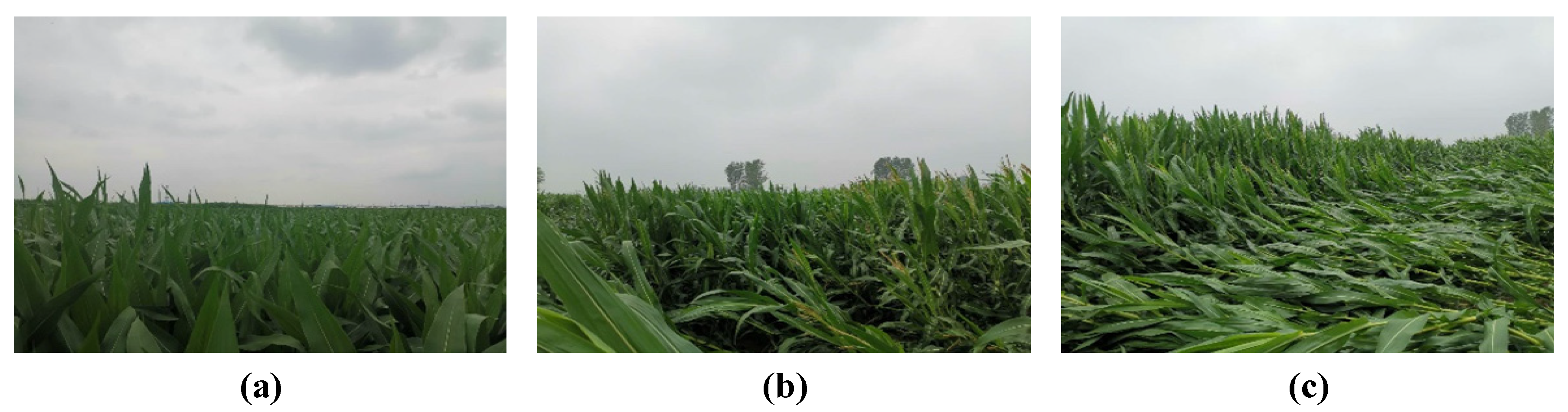
2.3. Field-Survey Data Acquisition and Lodging Type

Accurate classification of the various degree of lodging is vital for evaluating loss due to lodging and the resistance to lodging of the different maize varieties. The centimeter-scale image is helpful to distinguish different degrees of lodging of maize. Previous studies have proposed a variety of methods to classify the degree of lodging of maize. For example, Tian et al. [20] proposed a three-tier categorization system based on the angle between the upper stem and the main stem, with the tiers being the stem lodging, the root lodging, and the rhizome composite lodging. Combined with previous research and ground investigations, the lodging of maize in the present study area was divided into three degrees: non-lodging (NL), light lodging (LL), and severe lodging (SL), as shown in Figure 2 in the NL plot, the maize remains upright, which means that and the angle between the maize plant and its lodging varies from 60° to 90°. For LL, the angle between the maize plants before and after the lodging is 30° to 60°. Finally, for SL, the plant is close to or completely on the ground, the stem is completely exposed but not completely broken. After lodging, some leaves wither.

A grid of 2.5 m × 2.5 m was drawn on the maize experimental field and selected 116 grids, which covered all experimental categories evenly as quadrats (45 NL quadrats, 49 LL quadrats, and 22 SL quadrats). The number of quadrats, the GPS coordinates of the central point of each quadrat, and the degree of lodging of each quadrat (Figure 3) was recorded. All quadrats were used to analyze the characteristic factors associated with the different degrees of lodging and to evaluate the accuracy after lodging classification. In the process of classification, 60% of the samples were used as training samples, and 40% of the samples were used as validation samples.

2.4. UAV-RGB Image Preprocessing

First, the RGB aerial images obtained as per Section 2.1 were preprocessed, which included the following main steps (Figure 4):

(1)

Image filtering: To reduce the number of images and ensure good image quality, poor-quality images were deleted, such as those acquired during UAV takeoff and landing.

(2)

Image mosaic: To get the structural point cloud of the sparse scene, the GPS coordinates and the inertial navigation system attitude parameters recorded by the drone flight control system were combined, and Agisoft PhotoScan (Agisoft LLC, Saint Petersburg, Russia, version 1.4.5) was used to match the input image data based on the structure from motion algorithm (SfM) algorithm. Dense reconstruction then produced a dense point cloud. Next, the discrete three-dimensional points were connected to the polygonal mesh surface by surface reconstruction, and the texture was mapped to the surface to generate a realistic three-dimensional model. The final digital image served as the DSM [21,22,23]. Next, the ground control points obtained as per Section 2.2 served to make fine geometric corrections to the image of the study area. GCS_WGS_1984 served as the geographical coordinate system of the stitched RGB image, and the image was composed of red, green, and blue channels with each color containing eight bits (so the color value ranged from 0 to 255). The spatial resolution was 0.8 cm, and the image was stored in TIFF format.

(3)

Image clipping: ArcGIS 10.3 (Esri, USA) was combined with images and field-planting maps to outline the experimental types on the images, and cutting tools were used to remove parts that fell outside the study area, only the part of maize coverage is reserved, such as the base map in Figure 3.

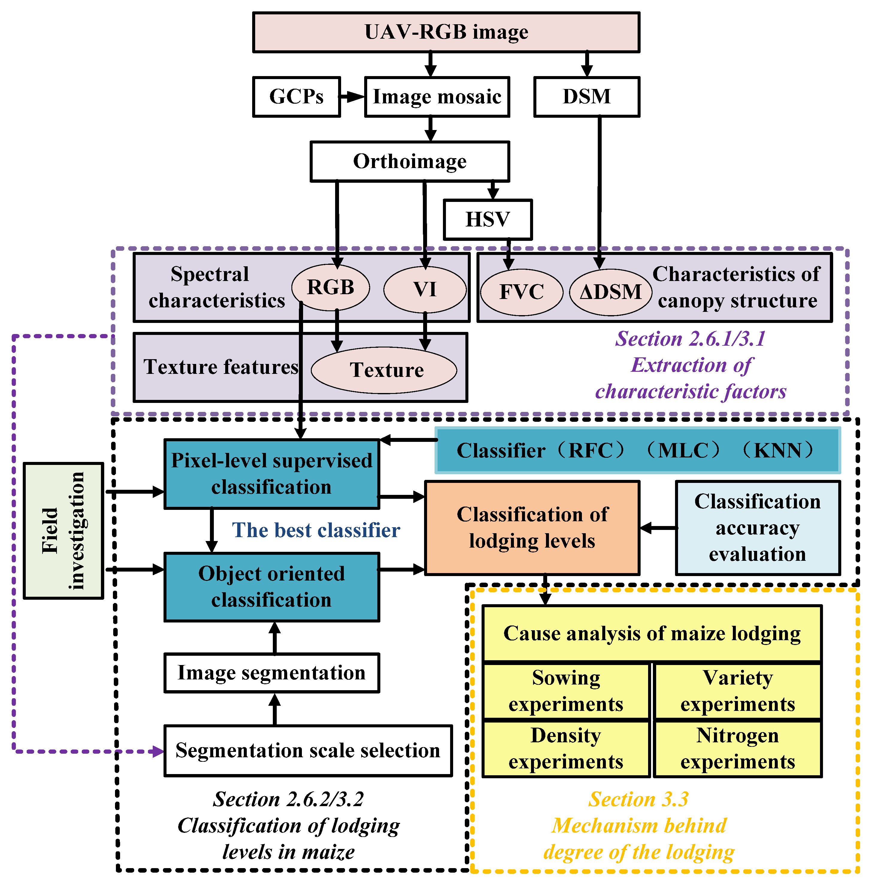
2.5. Technical Process of Study

The characteristic factors such as spectral reflectance, vegetation indexes, canopy coverage, and digital surface model depend on the maize lodging status. By combining these characteristic factors with the traditional pixel-level supervised classification method or object-oriented classification method, the maize lodging can be classified. The accuracy of the classification is evaluated by using the confusion matrix of validation samples. To better compare the advantages and disadvantages of the various classification methods, the experiment uses the same training samples and evaluation samples regardless of whether it uses pixel-level traditional supervised classification or object-oriented classification at the image object layer to extract lodging level.

This work uses the traditional classification method at the pixel level and tests and selects the best method to ensure that the best classifier is used in object-oriented classification. Under object-oriented conditions, only the combination of different feature factors is selected to determine the optimal classification combination. Combining the lodging-level classification maps with the highest classification accuracy from the various experimental research areas produces the spatial distribution of lodging, based on which the lodging-resistant maize varieties can be determined. In addition, this approach allows us to determine the risk of lodging as a function of planting density and nitrogen conditions. Figure 4 summarizes the process for classifying maize lodging.

2.6. Extraction of Maize Lodging

2.6.1. Extraction of Characteristic Factors for Different Degrees of Lodging of Maize

Three different maize lodging plots were selected from within the 116 plots in the RGB image (see Section 2.3). The spectral characteristics, texture characteristics, and differences in canopy surface, vegetation coverage differences, and other characteristic factors were calculated and statistically analyzed. The characteristic factors that proved useful for distinguishing between the different degrees of lodging of maize were filtered out, and the degree of lodging was classified based on these factors.

(1)

Separation of soil background and extraction of canopy coverage

Although most of the canopy was in the VT (tasseling) or V14 stage of maize, the images show that the canopy coverage and leaf distribution pattern still depended strongly on the degree of lodging. For one thing, the soil affects the spectral reflectance, thus affecting the vegetation index. In addition, the distribution pattern of soil gaps or leaves can reflect the degree of lodging of maize.

The spatial distribution of HSV (hue, saturation, value) color served to separate soil background, and its components are usually used as feature vectors for image classification and image recognition [24]. Note that the HSV color space is a subjective space where H represents hue, S represents saturation, and V represents value. Thus, for this paper, the image was transformed from RGB color space to HSV color space. Compared with the RGB color space, color segmentation of the image in HSV space produces more intuitive brightness and hue, which allows the naked eye to detect differences between colors by inspection. The specific conversion formulas are as follows [25,26]:

$$H_1={\cos }^{-1}\left\{\frac{0.5\left[R-G+(R-B)\right]}{\sqrt{{\left(R-G\right)}^2}+\left(R-B\right)}\right\},$$

(1)

$$H=\left\{\begin{array}{c}{H}_1\\ {360}^{\circ }-H_1\end{array}\begin{array}{c} \mathrm{if}B\le G\\ \mathrm{if}B>G\end{array}\right.,$$

(2)

$$S=\frac{\max (R,G,B)-\min (R,G,B)}{\max (R,G,B)},$$

(3)

$$V=\frac{\max (R,G,B)}{255}.$$

(4)

Once the image was transformed into HSV space, H, S and V color histograms were extracted and their color features analyzed. The ranges of H, S, and V determine the pixel color. After numerous experiments, the intervals of the three components of H, S, and V for green were determined to be [26~34], [43~255], and [46~255]. Pixels in this interval were classified as vegetation pixels, and pixels not in this interval were classified as gap elements.

The extracted vegetation coverage layer was used to mask the original image to obtain RGB images with soil background removed, such as Figure 4 and Figure 5a, where Figure 5a and Figure 4 is before (after) lodging. The images of different degrees of lodging after lodging differ significantly from those before lodging. Figure 4 and Figure 5c shows the result of vegetation coverage before (after) lodging. Combining Figure 5b with the classification results after lodging shows that the distribution of vegetation coverage in SL images exhibits a clear directionality, and the vegetation coverage increases significantly. The images without lodging show a clear and obvious canopy structure, and the gap distribution of vegetation is relatively uniform. Therefore, the data on vegetation coverage can be used as a feature factor for lodging classification.

(2)

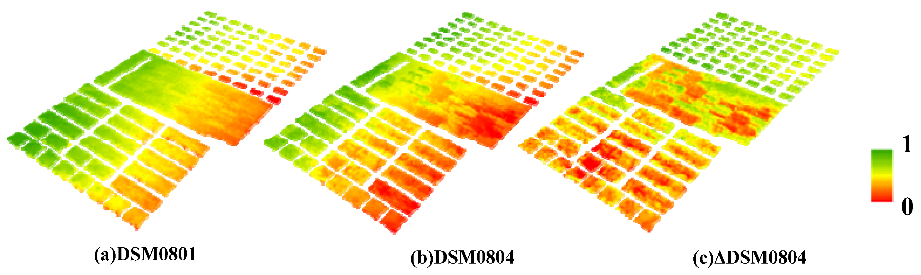
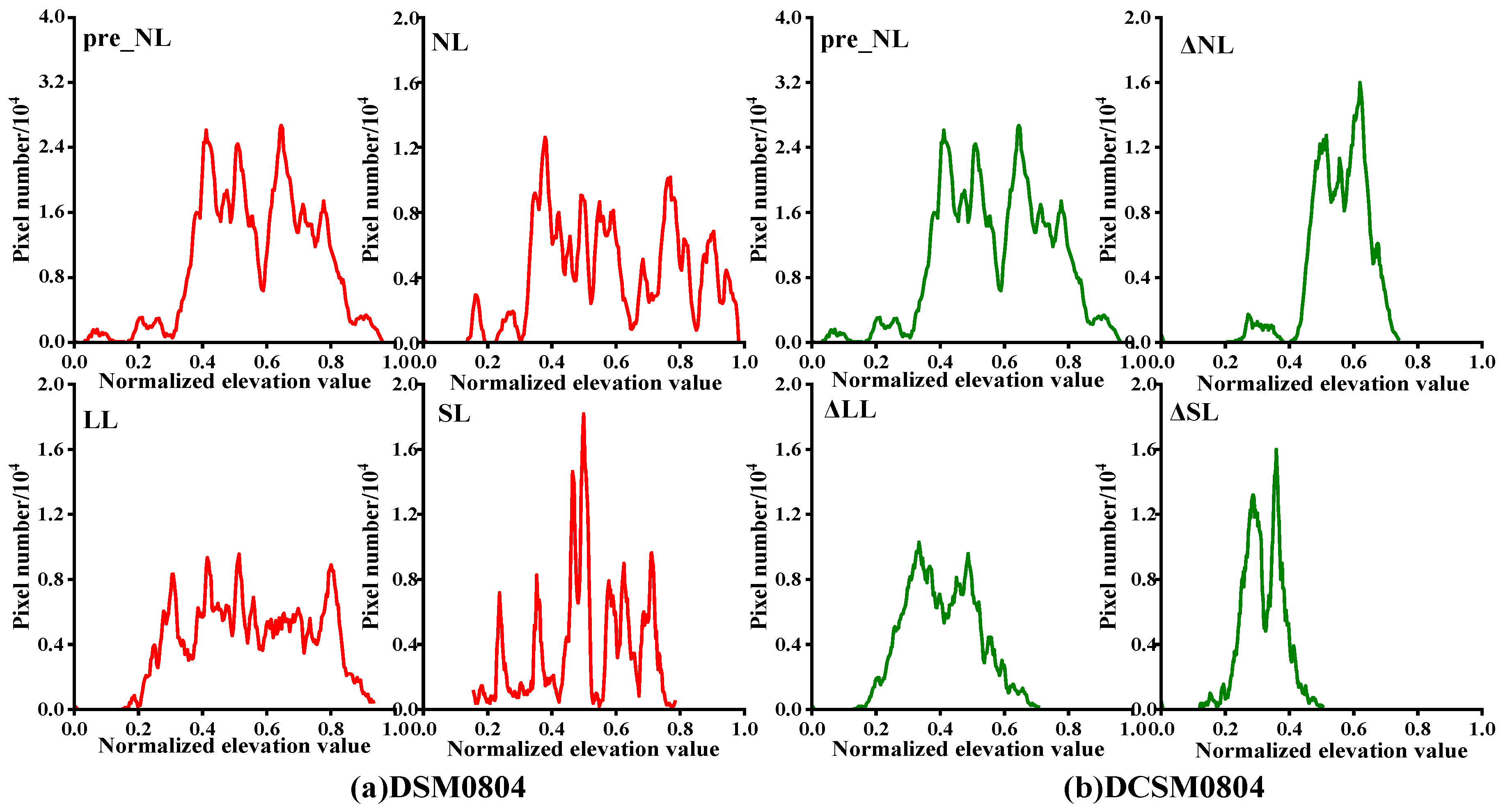
Construction of digital elevation model and generation of digital surface model

In step 2 of Section 2.4, the generation of orthophoto in the study area allowed us to create a DSM before and after lodging based on the three-dimensional point cloud reconstructed by using the structure-from-motion algorithm. The DSM shows how the ground height fluctuates in the study area. However, because no digital elevation model of the bare land (i.e., before planting) was available, the absolute height of the maize plant could not be obtained, so the relative elevation was used to describe the fluctuation of canopy height. The original DSM was masked with the plot boundary drawn before so that the DSM after the mask includes only the changes in the maize canopy (i.e., before and after lodging) but does not include the height of the land. For the maize canopy model under different lodging conditions without the soil height, a fuzzy degree of membership was used to normalize the original DSM to (0, 1). Here, a linear classification function was used. By applying the same method, the 1 August (pre-lodging) and 4 August (post-lodging) digital surface models were obtained. These images show that the terrain on the west side of the study area is higher than that on the east side, which indicates that fluctuations in absolute elevation will seriously affect the lodging classification based on a DSM (Figure 6a,b). Therefore, differences between the pre- and post-lodging data were calculated to obtain the relative changes in the digital surface model due to lodging. Consistent with the previous operation, membership ambiguity served to normalize the change of this elevation to (0, 1), as shown in Figure 6.

(3)

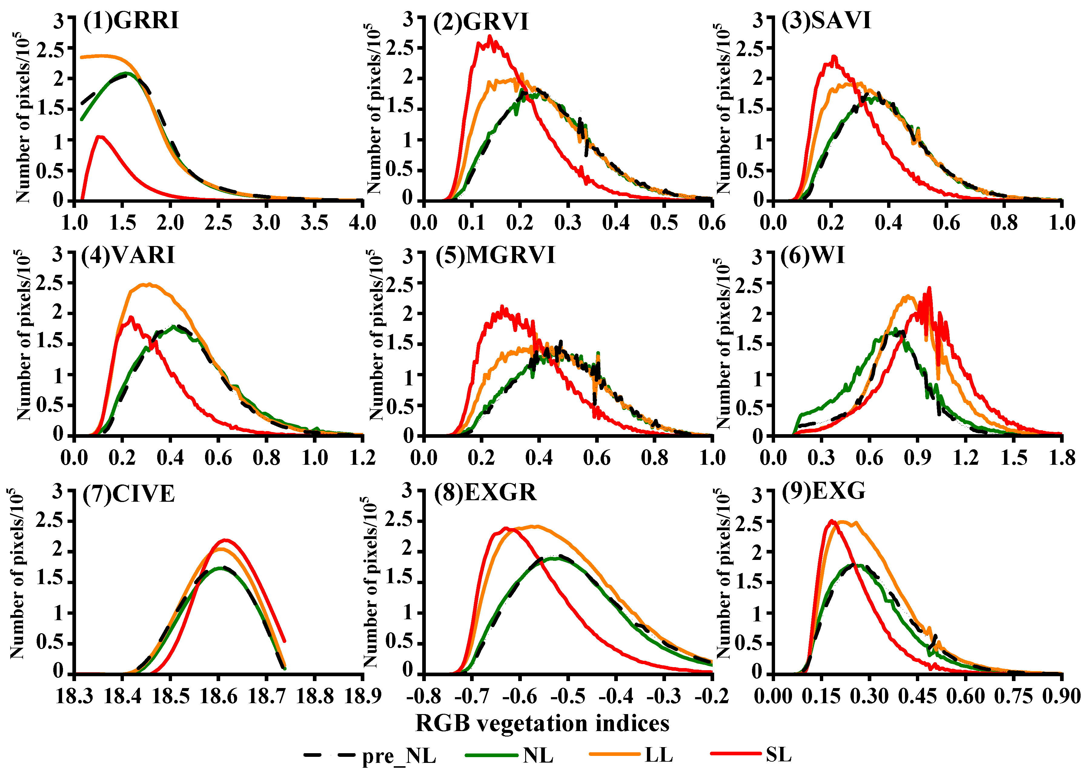
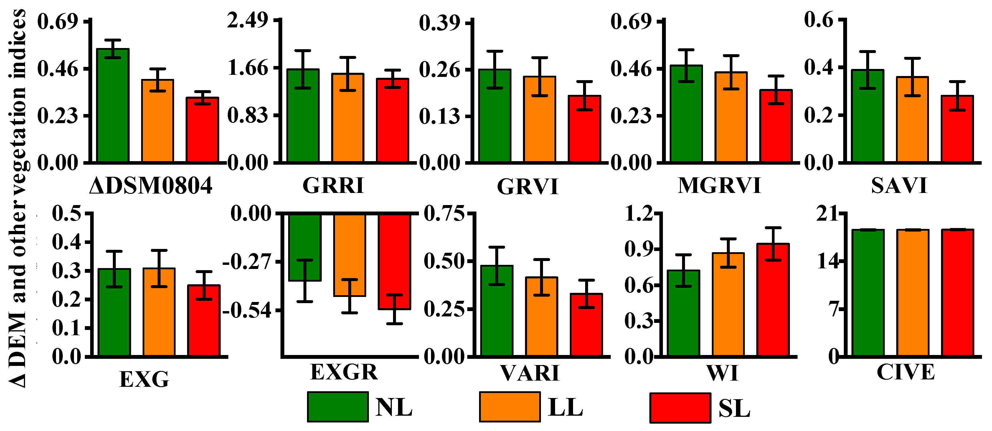
Construction of vegetation indices

The vegetation indices can enhance the interpretation of remote-sensing images by linearly or nonlinearly combining two or more characteristic bands, which allows it to play a significant role in crop-growth detection and fine classification. Several commonly used vegetation indices were selected to enhance the gap between different levels of maize after lodging. The results showed that the green and blue bands increased more with increasing degree of lodging. Therefore, a vegetation index constructed from the blue and green bands was devised to detect the difference between the degrees of lodging. Previous studies also showed that the green band correlates more closely with the physical and chemical parameters of vegetation [27].The excess green index (EXG) and excess green minus excess red index (EXGR) are two common visible vegetation indices. Woebbecke (1995) [28] found that EXG provides a near-binary intensity image outlining a plant region of interest, and that the vegetation data can be extracted by threshold segmentation. The color index of vegetation extraction (CIVE) integrates the information in the red, green, and blue bands to enhance the vegetation information. In addition, the green-red ratio index (GRRI), green ratio vegetation index (GRVI), modified green-red vegetation index (MGRVI), visible atmospherically resistant index (VARI), and Woebbecke index (WI) changed the linear exponential form into the ratio form to enhance the difference between degrees of lodging. The soil-adjusted vegetation index (SAVI) is less sensitive to soil than the traditional vegetation index, thereby reducing the impact of soil. The formulas for these nine vegetation indices are given in

Table 4. Characteristic bands or vegetation indices used in this experiment.

Abbreviation	Full Name	Formula	Reference
$r$	Normalized red intensity	$r=R/(R+G+B)$	Kawashima et al., (1998) [29]
$g$	Normalized green intensity	$g=G/(R+G+B)$	Kawashima et al., (1998) [29]
$b$	Normalized blue intensity	$b=B/(R+G+B)$	Kawashima et al., (1998) [29]
GRRI	Green-red ratio index	$GRRI=G/R$	Gamon et al., (1999) [30]
GRVI	Green ratio vegetation index	$GRVI=(g-r)/(g+r)$	Tucker et al., (1979) [31]
SAVI	Soil adjusted vegetation index	$SAVI=\left(1+L\right)\times \frac{\left(G-R\right)}{G+R+L},L=0.5$	Li et al., (2010) [32]
MGRVI	Modified Green Red Vegetation index	$MGRVI=(g^2-r^2)/(g^2+r^2)$	Bendig et al., (2015) [33]
VARI	Visible atmospherically resistant index	$VARI=(g-r)/(g+r-b)$	Gitelson et al., (2002) [34]
WI	Woebbecke index	$WI=(g-b)/\left|r-g\right|$	Woebbecke et al., (1995) [35]
CIVE	Color index of vegetation extraction	$CIVE=0.441r-0.811g+0.385b+18.78745$	Kataoka et al., (2003) [36]
ExG	Excess green index	$ExG=2g-r-b$	Woebbecke et al., (1995) [35]
ExGR	Excess green min us excess red	$ExGR=ExG-1.4r-g$	Guijarro et al., (2011) [37]

.

(4)

Statistics and analysis of texture features

The ground features on the high-precision lodging maize plots obtained by drones have a single category, and the difference in waveband information and RGB vegetation index under different lodging levels is limited, but from the change in canopy coverage, the texture characteristics are quite obvious. The texture characteristics of the ground objects in the image can be obtained by processing with different texture filters. This method can better treat the problem whereby foreign objects produce the same spectrum, thereby improving the accuracy of classification.

The gray level co-occurrence matrix (GLCM) provides a comprehensive analysis of the local features and a pixel-based arrangement. It reflects the distribution of the image gray level and presents repeated, alternating, or specific spatial rule changes, which is the basis for obtaining image texture features [38]. It also describes the probability that a pair of pixels separated by d pixels in the direction θ had gray level i and j, so the element can be denoted P (i, j | d, θ) or, when θ and d are selected, as P_{i, j.} The red, green, and blue bands are standardized, so the RGB vegetation indices (VARI, MGRVI, SAVI, and GRVI) were used from Section 2.6.1 to do texture filtering by calculating the gray level co-occurrence matrix. This gives us the mean, variance, homology, contrast, dissimilarity, entropy, second moment, correlation, etc. (there are 56 texture features altogether) [14]. The window for the second-order probability filter is set as 7 × 7, the transform components of the spatial correlation matrix X and Y are 1 and 1, and the gray quality level is 64.

To select high-quality texture features, the mean and variance of the texture features of 45 NL, 49 LL, and 22 SL samples are counted, from which we calculated their respective coefficients of variation and the different coefficient of LL and SL relative to NL (see calculation in Appendix A). The calculation is as follows [15]:

$$V=\frac{D}{M}\times 100\%,$$

(5)

$$D_w=\frac{S_1-S_2}{S_2}\times 100\%,$$

(6)

where D is the variance, V is the coefficient of variation, M is the sample mean, D_w is the difference coefficient, and S₁ and S₂ are the mean values of samples 1 and 2, respectively. Here the strategy of the texture feature factor was used to choose the degree of lodging with a high degree of internal aggregation and of dispersion between degrees of lodging; in other words, larger difference coefficients and smaller coefficients of variation provide better results.

2.6.2. Extraction Lodging from Maize Field with Different Degrees of Lodging

(1)

Classification of Maize Lodging by Pixel-Level Supervised Classification

Pixel-level supervised classification selects the sample pixels of the confirmed category, uses the sample pixels to train the discriminant function, and then compares the other pixels with the trained discriminant function to classify them into the most similar sample class according to various rules. First, three classical classification methods were selected to classify the RGB images after separating out the soil background. The maximum likelihood classification assumes that each class of statistics in each band is normally distributed. The likelihood of a given pixel belonging to a certain training sample was calculated, and then the pixels were merged into the maximum-likelihood category [39]. The K-nearest-neighbor method classifies images according to Euclidean distance between the data to be classified and the training-area elements in n-dimensional space. The number of object attributes obtained during classification was denoted N. Compared with the traditional nearest-neighbor method, the K-nearest-neighbor method produces smaller sensitive outliers and noise data sets and thus obtains more accurate classification results. It automatically determines to which category pixels most likely belong [40]. Random forest classification (RFC) integrates multiple trees by using ensemble learning [41]. Its basic unit is the decision tree, and each decision tree is a classifier. For an input sample, n trees will have n classification results. RFC integrates all the classification voting results and specifies the category with the greatest number of votes as the final output, thereby improving the classification accuracy [42].

To obtain the classification, we first remove the small patches from the classification results and smooth the boundary to clarify the classification. Next, 70 of 116 sample cells were used (i.e., 60%) as training samples and 46 (40%) as validation samples to evaluate the results. The method most used to evaluate the classification accuracy of remote-sensing images is to establish the confusion matrix for statistical analysis. This matrix can be used to calculate the producer’s accuracy, the user’s accuracy, the commission error, and the omission error for each category, as well as the overall accuracy and the kappa coefficient of the entire classification result. This work uses high overall representative accuracy and kappa coefficient as evaluation indexes. Overall accuracy reflects the probability of consistency between the classification results and the real ground results, and the kappa coefficient serves as an index to judge whether the two images are consistent. The Kappa coefficient ranges from −1 to 1, but it is usually between 0 and 1. The closer the Kappa coefficient is to 1, the higher the classification accuracy.

(2)

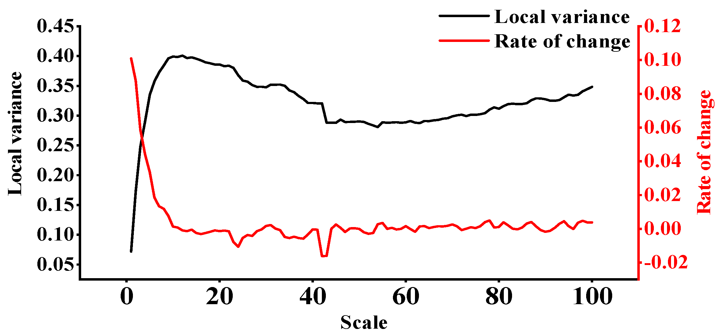
Classification of Maize Lodging by Object-Oriented Classification

Section 2.6.1 discusses the extraction of the vegetation index, texture characteristics, digital surface model (DSM), and vegetation canopy coverage under different degrees of lodging. These characteristic bands and object-oriented classification methods were combined to classify the degree of the maize lodging. Due to the high resolution of the acquired images, the traditional supervised classification method increases the fragmentation of the classification result at the pixel-level, which complicates the boundary. The object-oriented classification method can greatly improve this situation by segmenting the image and establishing classification rules. Image segmentation is affected by both the segmentation scale and the segmentation algorithm, and the results of segmentation directly affect the accuracy of object-oriented classification.

3. Results

3.1. Extraction of Multi-Feature Factors from RGB Images

After removing the soil background and marking the vegetation-covered pixels with one and the remaining pixels with zero, the binary image was obtained as explained in Section 2.6. Next, the percent accumulation histogram shown in Figure 7 combines the 116 sample plots with three lodging levels. The ratio of area covered by vegetation to total area is the fractional vegetation cover (FVC), which is also considered as the part with the value of one on the binary image, and the ratio of the remaining area (i.e., the area not covered by vegetation) to total area is the gap fraction (GF), which is the part with the value of zero on the binary image. The sum of the vegetation coverage and clearance rate in each area is unity, and the vegetation coverage increases with increasing degree of lodging. Compared with the day before lodging, the vegetation coverage of NL areas decreased slightly on the day of lodging, which may be due to cloud-induced shadows appearing when the image was collected on the day after lodging.

Like the method used to evaluate vegetation coverage, the digital canopy model of 116 sample plots before and after lodging was statistically analyzed to understand the changes caused by lodging. Figure 8 shows the histogram of the elevation of different lodging plots as determined by the DSM, where the vertical axis gives the number of pixels for each height on the horizontal axis. Figure 8a shows the results for NL, LL, and SL, and Figure 8b shows the difference between the two DSMs, which can also be divided into the change due to lodging for NL, LL, and SL (denoted ∆NL, ∆LL, and ∆SL). The terrain factors produce an irregular multi-peak distribution in the gray histogram. Subtracting the difference ΔDSM0804 between the two images (before and after lodging) reveals a single-peak distribution or double-peak distribution in the gray histogram. With increasing degree of lodging, the peak shifts toward lower elevations. Combining this result with the image in Figure 6c shows that ∆DSM also offers unique advantages for describing crop lodging. However, the disadvantage is poor accuracy, which arises because the error is amplified by flight weather and absolute terrain fluctuations. In general, the change produced in the DSM due to lodging can also be a good characteristic factor. A reasonable threshold segmentation of ΔDSM0804 can provide the classification result for degree of maize lodging. Combining the peak and segmentation of the gray histogram of ΔDSM0804 under different degrees of lodging produces final classification elevations of 0.35 and 0.52. The accuracy of the classification results is evaluated together with the other classification methods.

The reflectance is modified as a function of the degree of lodging of maize. This section discusses the characteristic factors related to the degree of lodging from the perspective of the reflectance spectrum. First, the orthorectified RGB data was standardized: 116 sample cells were used to produce the gray histogram of the three bands for the different degrees of lodging (Figure 9). The number of pixels in the red, green, and blue bands from the NL plot is basically the same before and after lodging (Figure 9a,b). For SL, the peak value of the blue band is lower than the red band, and the peak value of the red band is much lower than the green band. With increasing degree of lodging, the peaks of the three bands shift to higher gray values; that is, the reflectivity changes, and the gray value of the green band increases significantly. According to the histogram of the mean change for the different degrees of lodging (Figure 10), the reflectivity of each band increases by 8.49–17.95% for moderate lodging, and by 21.91–38.99% for SL.

Figure 11 shows the histogram of each vegetation index calculated for the sample plot with different degrees of lodging. The abscissa gives the vegetation index, and the ordinate gives the number of pixels. The gray histograms of the vegetation indexes for different degrees of lodging show the distribution of the single peak. With increasing degree of lodging, the peak of the histograms of the GRRI, GRVI, MGRVI, SAVI, EXGR, and VARI all shift to the lower values, whereas the peak value of the WI shifts to higher values. Combining these results with the change in the average pixel value for each degree of lodging (Figure 12) shows that the CIVE and GRRI remain relatively unchanged as the degree of lodging increases. As with the change ∆DSM0804 from the digital surface model, the trends of GRVI, MGRVI, SAVI, EXGR, and VARI correlate negatively with degree of lodging, whereas WI correlates positively with degree of lodging. The change in EXG increases first and then decreases. Furthermore, the change in ExG is inconsistent with the increasing degree of lodging, and the different levels in the histogram of WI and EXGR cross each other so that the distributions of these indices in their histograms are not centralized. Therefore, GRVI, MGRVI, SAVI, and VARI are chosen as characteristic factors for classifying the degree of lodging.

About the selection of texture features, first, they were arranged in reverse order according to the relative difference coefficients of LL and SL with respect to NL. Features with difference coefficients greater than 25% were selected and then sorted by the coefficient of variation of NL, LL, and SL. The results show that green_mean and green_homogeneity produce the most accurate classifications, with the results of mgrvi_variance, vari_variance, and vari_contrast producing slightly less accurate but still acceptable classifications. Thus, these five texture features were used as the optimal feature factors to classify the degree of lodging.

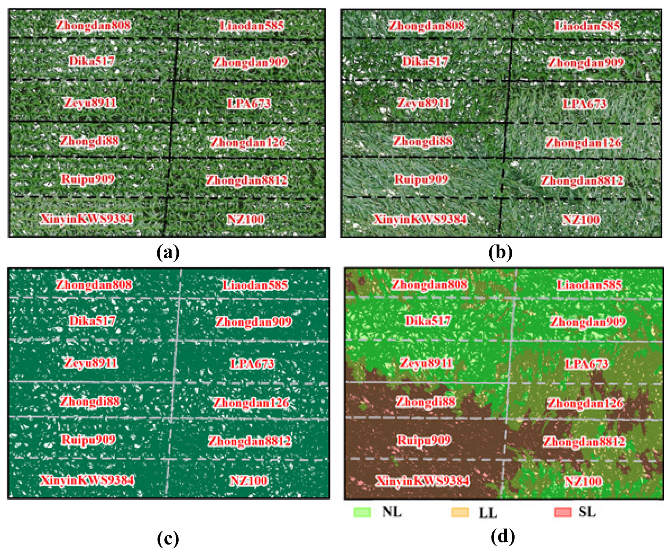
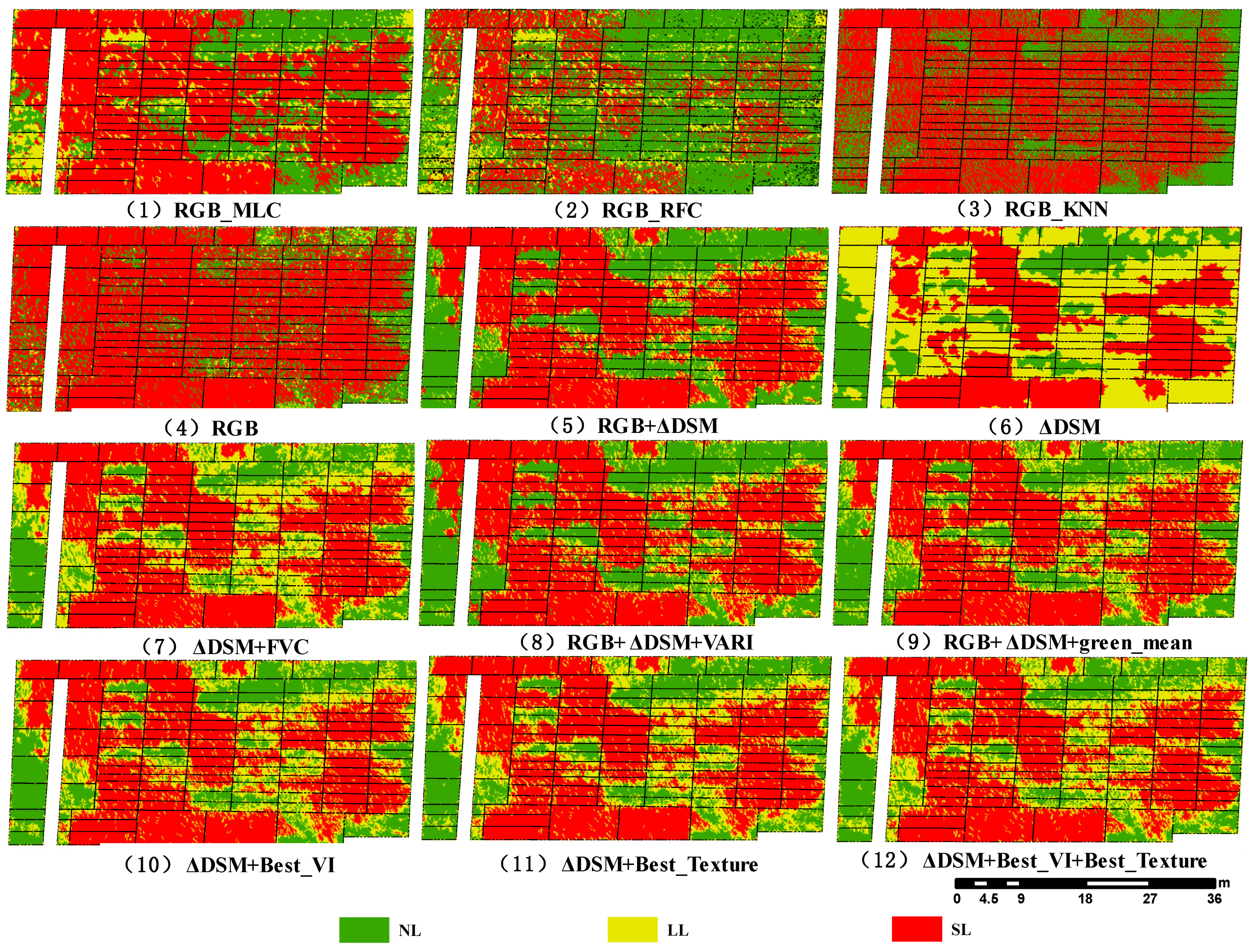
3.2. Classification of Each Degree of Lodging by the Various Classification Methods

The supervised classification tool of ENVI 5.3 (Exelis, Broomfield, CO, USA) was used to achieve pixel-level classification. In addition to RFC, the two classification methods adopt default parameters. For the RFC method, the random forest classification tool in ENVI extension tool was used to implement [42].The specific parameter settings are as follows: the number of trees is 50; the number of features adopts the default “square root” method, that is, number of features = sqrt (NB), where NB is the number of bands of the input image to be classified; minimum number of samples to stop splitting is 5; minimum integrity to stop splitting is 0.Of the three pixel-level supervised classification methods, RFC is the most accurate. Its overall accuracy is 78.26%, and the kappa coefficient is 0.6098, RFC was used to classify images after removing the soil background.

For object-oriented classification, firstly, the optimal segmentation scale can be determined by using the estimation-of-scale parameters algorithm [43], which iteratively segments images from bottom to top on multiple scales and calculates the local variance (LV) between objects for each image-object layer. The rate of change in LV (ROC-LV) is then used to magnify the mutation of LV, and the maximum ROC-LV reflects the candidate values for the best segmentation scale, as shown in Figure 13 By using these candidate values, the optimal segmentation scale is determined to be Since the digital surface model ∆DSM0804 has been normalized, we give it a weight of 20 for its participation in segmentation and weight the other feature bands as Considering the edge smoothness and compactness of the segmentation object, the smooth compactness parameter is set as 0.5 to obtain the segmentation result. In the process of object-oriented extraction of maize with various degrees of lodging, the basic classification unit is the object with various attributes generated after image segmentation. This differs from the pixel in traditional image-supervised classification, which provides a higher-level classification. RFC, which is the best pixel-level supervised classification method, was chosen to use object-oriented classification in the image layer in this section.

Then, this study used eCognition Developer (Definiens Imaging, Germany, version 9.0) to achieve the object-oriented classification. The selection of classifier is RFC, the depth of tree is 20, the number of trees is 50, and other parameters use default parameters. Different band combinations were selected for classification, with the results shown in Figure 14 RFC produces the best classification of the three pixel-level classification methods. The maximum likelihood classification and K-nearest-neighbor method caused a certain degree of misclassification for LL and SL. The former underestimates the fraction of NL, and the latter does not detect LL. The fraction of LL in the hierarchical distribution obtained by threshold segmentation using ∆DSM increases significantly, which is due to the poor horizontal and vertical accuracy of ∆DSM. The results of object-oriented classification show that the combination of ∆DSM, FVC, VI, and texture improves the classification results, and the fragmentation and noise in the classification results can be significantly improved. Different classification results are evaluated combined with the accuracy evaluation method in Section 2.6.2.

Table 5. Classification accuracy for various classification methods and combinations of characteristic bands.

Classification Method		Characteristic Band Combination	Overall Accuracy	Kappa Coefficient
Threshold segmentation		∆DSM	78.26%	0.63
Pixel-level supervised classification		RGB (max likelihood classification)	60.87%	0.43
		RGB (RFC)	78.26%	0.63
		RGB (K nearest neighbor)	56.52%	0.33
Object oriented classification	Based on spectral data	RGB	45.65%	0.28
		RGB+∆DSM	82.61%	0.72
	Based on canopy structure data	∆DSM+FVC	80.43%	0.68
	Based on vegetation index	RGB+∆DSM+GRVI	82.61%	0.72
		RGB+∆DSM+MGRVI	80.43%	0.69
		RGB+∆DSM+SAVI	65.22%	0.47
		RGB+∆DSM+VARI	86.96%	0.79
	Based on texture features	RGB+∆DSM+green_homogeneity	80.43%	0.68
		RGB+∆DSM+green_mean	86.96%	0.79
		RGB+∆DSM+w_mgrvi_variance	84.78%	0.75
		RGB+∆DSM+vari_contrast	80.43%	0.68
		RGB+∆DSM+vari_variance	86.96%	0.78
	Without original RGB image	∆DSM+Best_VI	86.96%	0.78
		∆DSM+Best_Texture	84.78%	0.74
		∆DSM+Best_VI+Best_Texture	84.78%	0.75

lists the overall accuracy and the kappa coefficient of the classification. The comprehensive classification of images indicates that the best vegetation index is VARI and the best texture feature is the green_mean. In addition, the highest classification accuracy is with the original RGB image, ∆DSM, and the green_mean. The overall classification accuracy is 86.96% and the kappa coefficient is 0.7931.

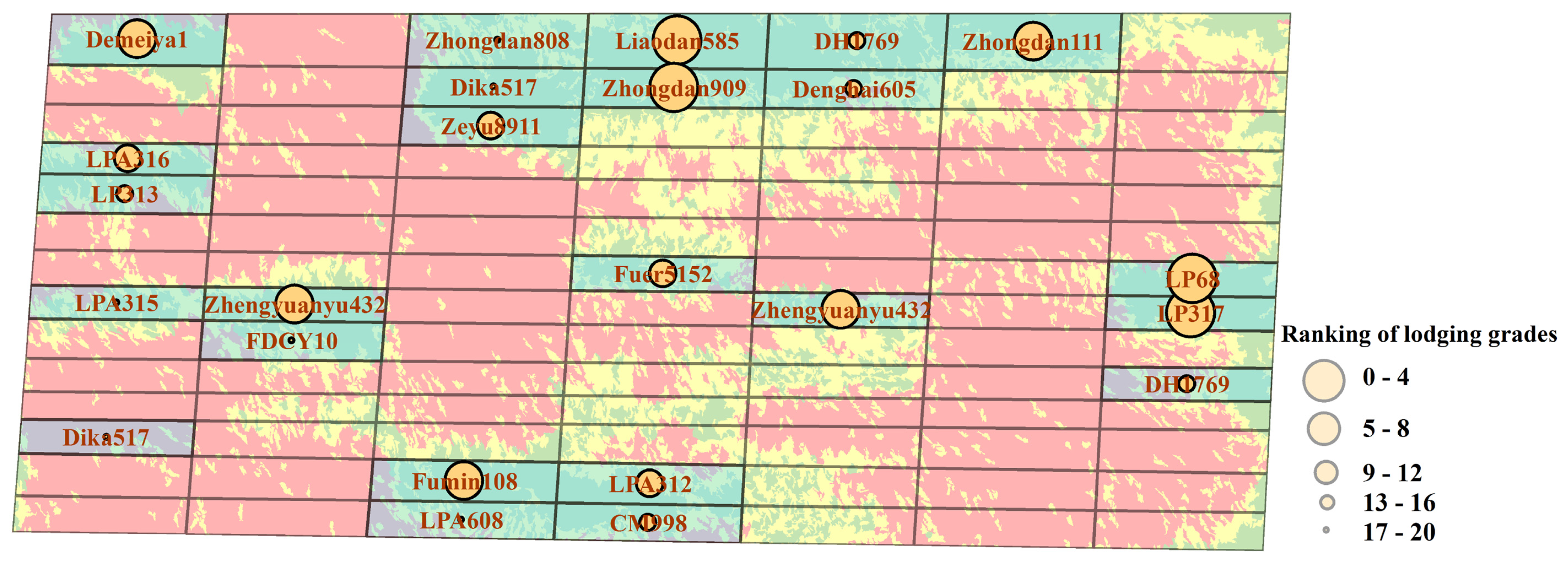
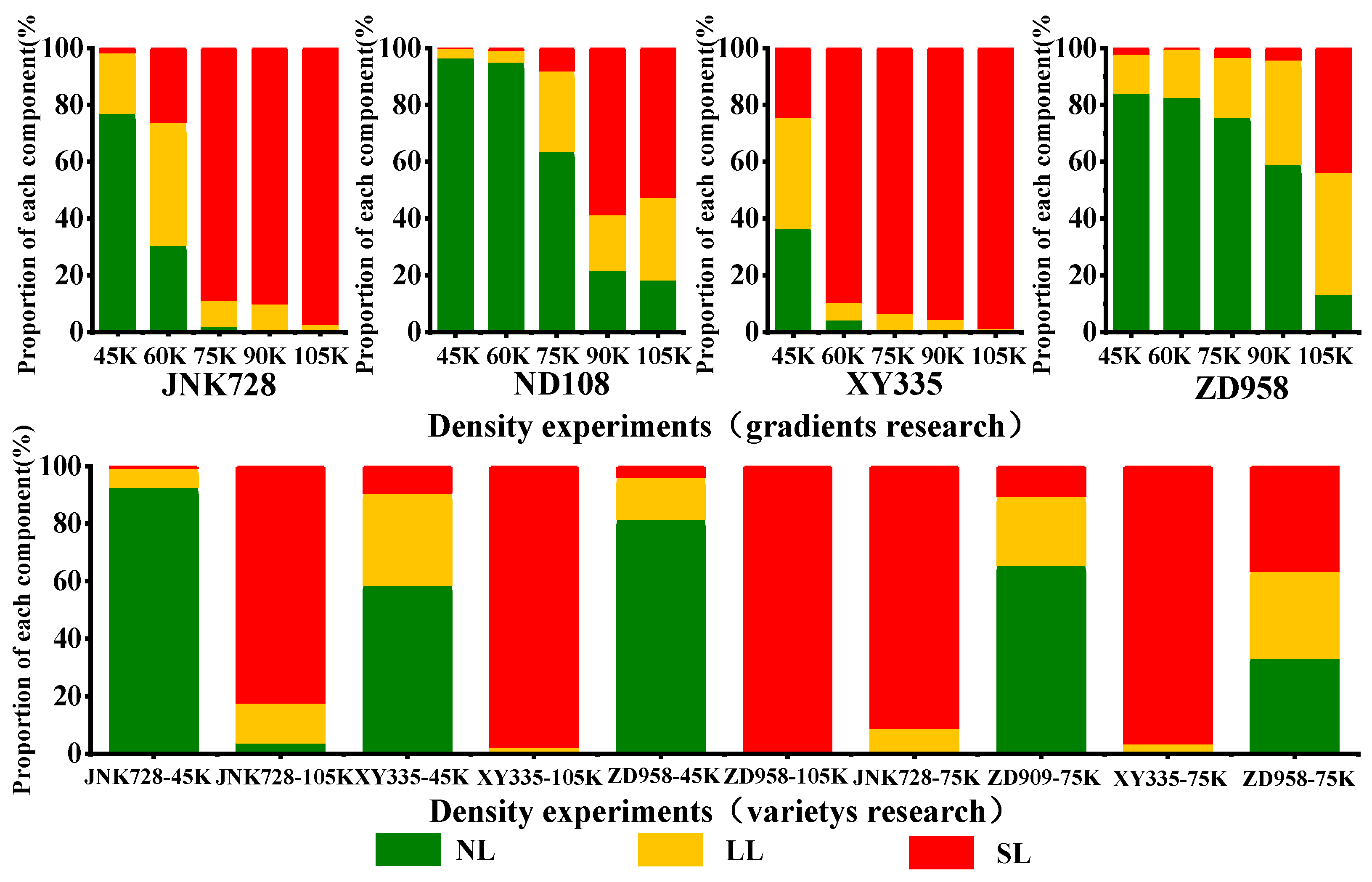
3.3. Mechanism behind Degree of the Maize Lodging

Based on the classification results from Section 3.2, the object-oriented classification method (RFC classifier) provides the most accurate classification of the combined features of RGB images, ∆DSM, and green_mean. To determine which factors most strongly influence maize lodging, the fraction of surface area that underwent lodging was calculated for each different maize variety, as well as for the different sowing dates, nitrogen treatment methods, and planting densities in the experimental field.

Figure 15 superimposes the degree of lodging onto the experimental plots. Green, yellow, and red plots correspond to NL, LL, and SL, respectively. The spatial distribution of maize with different degrees of lodging reveals a certain amount of lodging aggregation. The LL areas represent the smallest fraction of lodging type and are distributed along the boundaries between the NL and SL areas.

We applied a regional statistical analysis to the map of Figure 15 combined with the map of the maize variety to calculate the fraction of each maize variety that undergoes some degree of lodging. The top three varieties most resistant to lodging were Liaodan585, LP68, and Zhongdan909 (Figure 16). Figure 17 maps the top 20 varieties in terms of lodging resistance. Most of the maize varieties with zero lodging were located on the edge of the field, although a few were distributed in the center, such as Fuer5152 and Zhengyuenyu432, which indicates that these maize varieties offer superior resistance to lodging.

In the sowing-date experiment, the aisles or gaps between plots lead to a lodging fraction and degree of lodging that is far less than in the other experimental plots. These plots experienced only a small amount of LL and a small amount of SL. The lodging resistance of the three varieties remains essentially the same over the eight sowing dates. The fifth, sixth, and seventh stages are lodging-prone (i.e., R1, VT, and V14; see Figure 18).

Figure 19 compares the maize lodging under different nitrogen treatments. The results of nitrogen gradient treatment indicate that increasing the total nitrogen amount improves the lodging resistance of maize and decreases the fraction of SL. However, no significant change occurs in the range of NL.

The results of the operational experiment indicate that the fraction of NL of JNK728 and ZD958 was highest under nitrogen treatments N8–N Table 1 indicates that treatments N8–N10 are applied with base fertilizer in V5 and V6, N8 and N10 consisted of topdressing in stages V11 and V12, and N9 and N10 consisted of topdressing in the R1 silking stage. The results show that reasonable fertilization in the middle and late stages of maize vegetative growth is helpful to improve the lodging resistance of maize.

Figure 20 shows the fraction of NL, LL, and SL for various maize varieties at different planting densities. Combining these results with the degree-of-lodging map and the map of planting density reveals that a higher planting density reduces the fraction of NL. Both the density (gradient) and the density (variety) experiments shown that maize varieties JNK728 and XY335 have the worst lodging resistance. Varieties JNK728, ZD909, XY335, and ZD958 at 5K density were also tested, and the results show that ZD909 and ZD958 are more resistant to lodging. The proportion of LL and SL increases strongly with increasing planting density. Therefore, future research should focus on how to determine the planting density to best ensure stability, high yield, and lodging resistance.

4. Discussion

In this study, we developed a method to extract the degree of maize lodging based on multi-feature factors obtained from consumer UAVs and by applying an object-oriented classification method. In the following, we discuss in detail the basis for selecting characteristic factors, the evaluation of classification results, the factors that affect the degree of lodging, and the improvements of our experiment over previous work.

Regarding the selection of classification features, extracting feature factors for classification currently suffers from low accuracy in the early and late stages of maize growth, which may be due to the lower green-leaf coverage rendering the classification susceptible to soil, weeds, and field background [44]. However, extracting the green based on HSV color space can separate the above-ground objects from the maize, which produces good classification accuracy for degree of lodging. In addition, to improve classification accuracy, the vegetation index and texture index of the separated soil images can be used to enhance the difference between images with different degrees of lodging. Previous studies used a variety of sensors such as thermal infrared [11], LiDAR [45], and multispectral [14] to obtain various types of data with high sensitivity to different degrees of lodging. Furthermore, the different types of data enhance the differences between lodging and non-lodging crops. By applying classification algorithms that detect these differences, the lodging areas of different crops can be extracted.

However, the use of image features and object-oriented classification based on the original bands in UAV-RGB images produce a similar classification accuracy at a significantly lower cost. At the same time, Figure 7 shows that an increased degree of lodging results in increased canopy coverage. In addition, the vegetation canopy cover image obtained after the soil background separation is used as the characteristic layer, combined with the digital surface model to classify the degree of lodging, and the classification accuracy reaches 80.43%. This shows that the detection of lodging is more the detection of changes in the canopy structure, and we can achieve this goal by obtaining the information of the canopy structure more conveniently [12]. This conclusion shows that no matter what type of sensor is used (spectrum, lidar, and thermal infrared), the main target of feature selection is to extract the feature factors sensitive to canopy structure so that different degrees of lodging stand out significantly. Therefore, in future research, we will try to fuse different types of data to improve our ability to accurately identify crops with different lodging grades.

Extracting the key factors from images after separating out the soil background is vital for simplifying the detection of the maize lodging. Figure 11 and Figure 12 show that the GRVI, MGRVI, SAVI, and VARI indexes constructed based on the green and red bands provided clear advantages in extracting the degree of maize lodging. The results indicate that combining data from the green and red bands allows the degree of lodging to be monitored with precision. With increasing degree of lodging, the proportion of stem and vegetation index increased. This is because the reflectivity of each waveband increased to varying degrees after lodging [10]. Furthermore, the texture features are extracted by using the gray level co-occurrence matrix of the RGB image and several vegetation indexes, following which the optimal texture features are selected by applying a statistical analysis combined with the variation coefficient and the difference coefficient (see Appendix A) [15]. Moreover, some image feature factors in the image are strongly correlated. Choosing too many feature factors cannot improve the accuracy of the classification model.

Based on the classification results, the object-oriented classification is significantly more accurate than traditional pixel-level supervised classification, but also better than the results of threshold segmentation when relying only on ΔDSM. The reason for the low accuracy of the former is the high spatial resolution of the image obtained at low altitude, which leads to high image fragmentation after removing the soil background. In addition, the color of maize exposed to different degrees of lodging remains unchanged, so the low accuracy of ΔDSM is caused by the low accuracy of the digital surface model itself. Note that object-oriented classification using RFC combined with ΔDSM and vegetation coverage provides the best classification accuracy based on color features, which suggests the spatial distribution of degree of lodging may be obtained by relying only on high-precision canopy structure information. This is consistent with the results of Wilkes et al. [45], who combined the UAV canopy height model with the objective threshold method to obtain a quantitative expression of lodging rate and intensity. This result is also consistent with our conclusion in feature selection, which once again emphasizes the importance of obtaining canopy structure. In addition, the analysis of the canopy coverage obtained by removing the soil background and the texture features constructed by the vegetation index shows that the non-lodging maize is more evenly distributed, with fewer “gaps” or “holes,” and more homogeneous; the lodging maize has a clear directionality (pointing in one direction), and the length of the maize stalk displayed on the edge plots of the lodging part and the non-lodging part reflects the degree of lodging. However, this work still uses an object-oriented method to classify maize lodging by combining multiple feature factors on the image object layer. In future research, we will use this edge detection method to construct a look-up table in combination with varieties, nitrogen treatment, growth period, and other indicators to identify lodging-grade boundaries.

A major part of this research concerns the statistical analysis of maize with different degrees of lodging and under different field-management conditions. In addition, factors that affected the degree of lodging were also analyzed. Previous studies on the detection of lodging focused on single growth stages, and the experimental treatments, varieties, and cultivation methods were basically similar. For example, Wang et al. [10] studied the sensitivity of the vegetation index during the heading stage to obtain the degree of the maize lodging and used a dual-threshold division strategy to define a threshold to classify the severity of maize lodging. Since maize ears and grains begin to fill in the grain-filling stage, the vegetative growth basically stops, and, given the frequent summer storms, the grain-filling stage is prone to lodging. Li et al. [2] also studied how growth stage and type of lodging affected dry-matter accumulation, yield, and yield components of summer maize, and quantitatively evaluated the yield loss caused by lodging. In addition, they also proved that the stem lodging during the filling stage strongly affects maize yield. Therefore, this is also an important period for lodging detecting. The use of different sowing dates in the present study allows us to determine the growth stage that is the most prone to lodging. From other experimental plots, the optimal nitrogen-application strategy was also determined, as well as the optimal planting density and the most lodging-resistant variety.

The RGB images in this study have a higher spatial resolution and required a longer acquisition time than in previous studies. In future work, we will first obtain images with different resolutions and from different heights and then classify the degree of lodging by using the same method for optimizing UAV flight height and image resolution. Second, a more concise and comprehensive index was constructed in this work by combining different feature factors to monitor the degree of maize lodging. Finally, regarding the statistics of degree of lodging in different test regions, the maize lodging was affected not only by different treatments but also by the location at which the maize was planted, the distribution of fields, and the width of the aisles between plots.

In conclusion, maize lodging results from a host of environmental variables. Wen et al. [46] used a mobile wind machine to determine the lodging resistance of maize. However, the present method provides the true expression of lodging resistance of maize because the lodging classification under conditions of strong wind reflect the natural field conditions, which is consistent with the real environment in which crops grow. Of course, given a real experimental environment, many external factors are inevitable, such as the site terrain, the distribution of wind speed, and the width of the corridor in the experimental area. In future experiments, we must therefore evaluate traits that lead to real resistance of maize to lodging and comprehensively consider the external factors to determine the causes of maize lodging. This will help us better evaluate maize-lodging disasters and identify lodging-resistant maize varieties.

5. Conclusions

This paper uses UAV-RGB images with high spatial resolution and analyzes the spectral data before and after lodging. The vegetation index, texture features, canopy coverage, digital surface model, and characteristic spectral bands are constructed from visible bands and for different degrees of lodging. The combination of high-quality characteristic bands served as the basis for supervised classification and object-oriented classification methods to extract, with high precision, the degree of lodging. Based on experiments with different varieties, nitrogen treatments, densities, and sowing dates, the degree of lodging was divided into different regions. Finally, the factors that affect the maize lodging were analyzed from different directions according to the statistical results and spatial distribution of the degree of lodging. The results lead to the following conclusions:

(1)

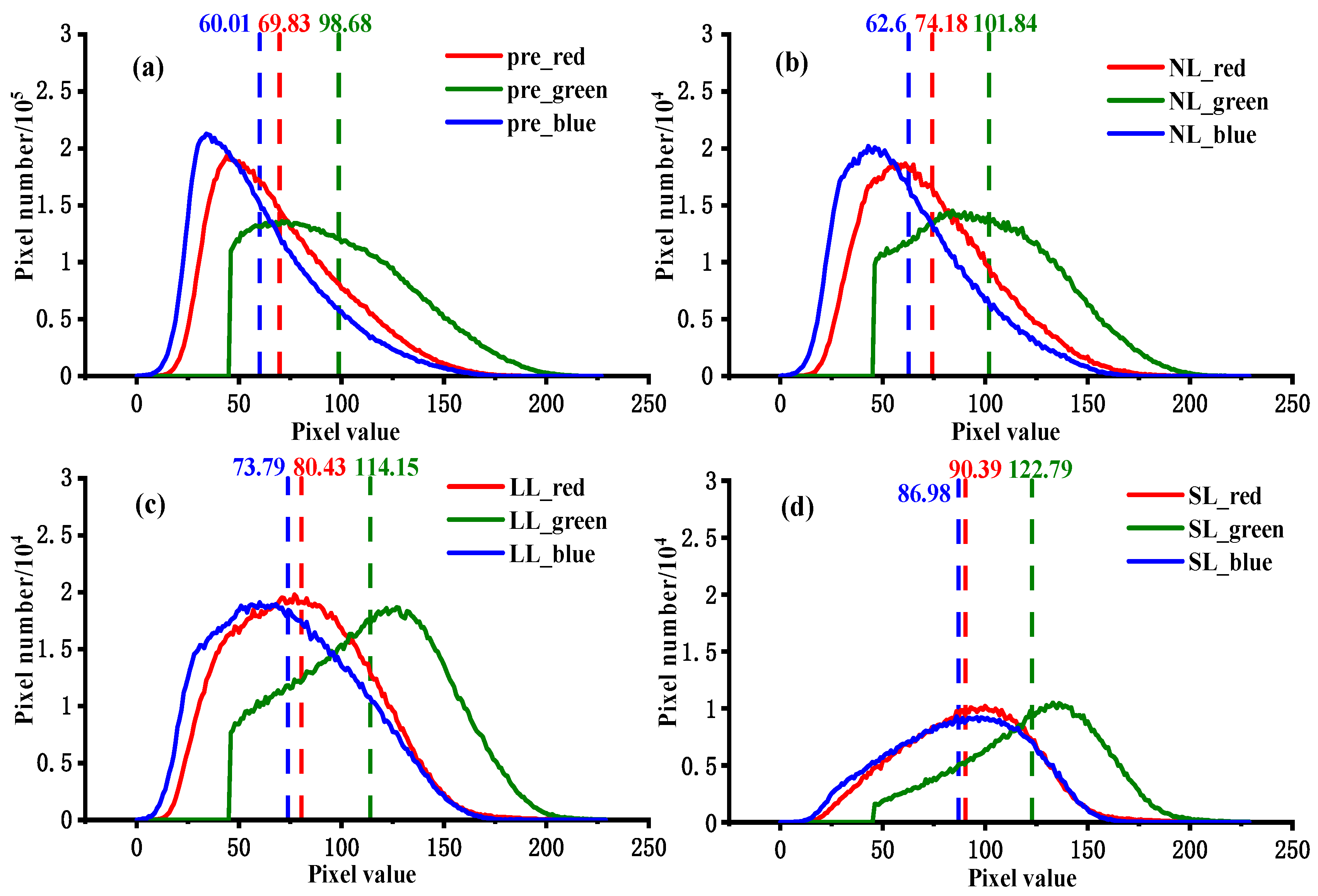
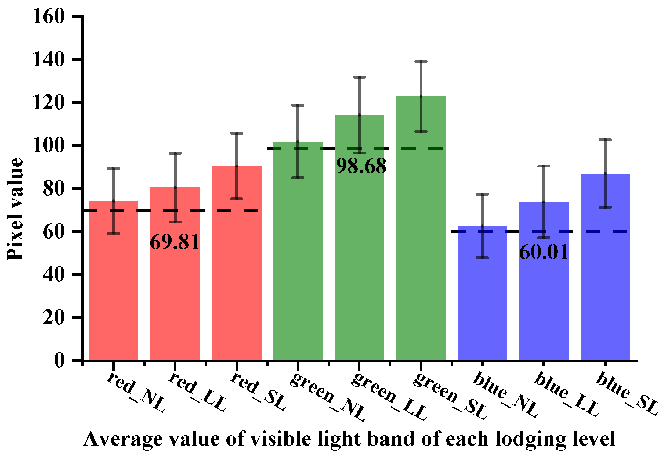
The maize lodging modifies to varying degrees the original reflectance spectrum, vegetation index, texture characteristics, canopy coverage, digital surface model, and other characteristic factors. A statistical analysis of these characteristic factors allows us to select the optimal vegetation index from GRVI, MGRVI, SAVI, and VARI and the best texture feature from green_mean, green_homogeneity, mgrvi_variance, vari_variance, and vari_contrast.

(2)

When using the supervised classification method to classify the degree of the maize lodging, although the samples are relatively independent of each other, the low discrimination of lodging maize on the pixel scale translates into a large number of non-green parts in the sample area, which leads to misclassification at the pixel level, resulting in a serious “salt-and-pepper phenomenon.” Even a posteriori removal of small patches does not significantly improve the classification results. In addition, supervised classification provides poor classification accuracy, which means that supervised classification methods applied to high-spatial-resolution images with significant differences in the category structure and similar color are valid only for general classification schemes.

(3)

When the object-oriented classification method is used, the input layers should first be segmented. This step fully extracts the spatial information in the image. At the same time, by exploiting the attributes of the segmented objects, we classify the objects according to the classification method by using the random forest classification method, which avoids the misclassification of pixels due to pixel-level classification of unified ground objects, thereby reducing the salt-and-pepper phenomenon. The result is clearer boundaries between the different degrees of lodging and improved classification accuracy.

(4)

Combined with the original image, digital surface model, and texture features, the overall accuracy of object-oriented classification method combined with random forest classification is 86.96%, and the kappa coefficient is 0.7931, which is the highest values of several classification methods. These results show that the method of extracting the degree of lodging of maize using UAV-RGB images combined with the derived feature factors is feasible and can be used to obtain greater classification accuracy.

Combining the results of the various experiments discussed herein indicates that maize is the most prone to lodging in R1, VT, and V14 stages, and that the degree of the maize lodging increases with increasing nitrogen application. In addition, the lodging resistance of maize also increases if fertilizer is applied in the middle and later stages of maize vegetative growth. These results reveal the three maize varieties most resistant to lodging are Liaodan 585, LP68, and Zhongdan909.

These experimental results provide an accurate delineation of degree of lodging, which should aid in detecting disaster losses. A better understanding of the factors that determine the degree of lodging can help us select lodging-resistant maize varieties, improve nitrogen treatments, and optimize planting density and sowing time.

References

1. Li, S.; Zhao, J.; Dong, S.; Zhao, M.; Li, C.; Cui, Y.; Liu, Y.; Gao, J.; Xue, J.; Wang, L.; et al. Research progress and Prospect of Maize Cultivation in China. Sci. Agric. Sin. 2017, 50, 1941–1959. [Google Scholar] [CrossRef]
2. Li, S.; Ma, W.; Peng, J.; Chen, Z. Study on Yield Loss of Summer Maize Due to Lodging at the Big Flare Stage and Grain Filling Stage. Sci. Agric. Sin. 2015, 48, 3952–3964. [Google Scholar] [CrossRef]
3. Berry, P.M.; Sterling, M.; Spink, J.H.; Baker, C.J.; Sylvester-Bradley, R.; Mooney, S.J.; Tams, A.R.; Ennos, A.R. Understanding and Reducing Lodging in Cereals. Adv. Agron. 2004, 84, 217–271. [Google Scholar] [CrossRef]
4. Chauhan, S.; Darvishzadeh, R.; Boschetti, M.; Pepe, M.; Nelson, A. Remote sensing-based crop lodging assessment: Current status and perspectives. ISPRS J. Photogramm. 2019, 151, 124–140. [Google Scholar] [CrossRef] [Green Version]
5. Yang, M.; Tseng, H.; Hsu, Y.; Tsai, H.P. Semantic Segmentation Using Deep Learning with Vegetation Indices for Rice Lodging Identification in Multi-date UAV Visible Images. Remote Sens. 2020, 12, 633. [Google Scholar] [CrossRef] [Green Version]
6. Salamí, E.; Barrado, C.; Pastor, E. UAV Flight Experiments Applied to the Remote Sensing of Vegetated Areas. Remote Sens. 2014, 6, 1051. [Google Scholar] [CrossRef] [Green Version]
7. Pádua, L.; Vanko, J.; Hruška, J.; Adão, T.; Sousa, J.J.; Peres, E.; Morais, R. UAS, sensors, and data processing in agroforestry: A review towards practical applications. Int. J. Remote Sens. 2017, 38, 2349–2391. [Google Scholar] [CrossRef]
8. Li, Z.; Chen, Z.; Wang, L.; Liu, J.; Zhou, Q. Area extraction of maize lodging based on remote sensing by small unmanned aerial vehicle. J. Agric. Eng. 2014, 30, 207–213. [Google Scholar] [CrossRef]
9. Wang, M.; Sui, X.; Liang, S.; Wang, Y.; Yao, H.; Hou, X. Simulation test and remote sensing monitoring of summer corn lodging. Sci. Surv. Mapp. 2017, 42, 137–141. [Google Scholar] [CrossRef]
10. Wang, L.; Gu, X.; Hu, S.; Yang, G.; Wang, L.; Fan, Y.; Wang, Y. Remote Sensing Monitoring of Maize Lodging Disaster with Multi-Temporal HJ-1B CCD Image. Sci. Agric. Sin. 2016, 49, 4120–4129. [Google Scholar] [CrossRef]
11. Liu, T.; Li, R.; Zhong, X.; Jiang, M.; Jin, X.; Zhou, P.; Liu, S.; Sun, C.; Guo, W. Estimates of rice lodging using indices derived from UAV visible and thermal infrared images. Agric. For. Meteorol. 2018, 252, 144–154. [Google Scholar] [CrossRef]
12. Han, L.; Yang, G.; Feng, H.; Zhou, C.; Yang, H.; Xu, B.; Li, Z.; Yang, X. Quantitative Identification of Maize Lodging-Causing Feature Factors Using Unmanned Aerial Vehicle Images and a Nomogram Computation. Remote Sens. 2018, 10, 1528. [Google Scholar] [CrossRef] [Green Version]
13. Chu, T.; Starek, M.J.; Brewer, M.J.; Murray, S.C.; Pruter, L.S. Assessing Lodging Severity over an Experimental Maize (Zea mays L.) Field Using UAS Images. Remote Sens. 2017, 9, 923. [Google Scholar] [CrossRef] [Green Version]
14. Sun, Q.; Sun, L.; Shu, M.; Gu, X.; Yang, G.; Zhou, L. Monitoring Maize Lodging Grades via Unmanned Aerial Vehicle Multispectral Image. Plant Phenomics 2019, 2019, 5704154. [Google Scholar] [CrossRef] [PubMed] [Green Version]
15. Guo, P.; Wu, F.; Dai, J.; Wang, H.; Xu, L.; Zhang, G. Comparison of farmland crop classification methods based on visible light images of unmanned aerial vehicles. J. Agric. Eng. 2017, 33, 112–119. [Google Scholar] [CrossRef]
16. Wang, X.; Wang, M.; Wang, S.; Wu, Y. Extraction of vegetation information from visible unmanned aerial vehicle images. J. Agric. Eng. 2015, 31, 152–157. [Google Scholar] [CrossRef]
17. Li, N.; Zhou, D.; Zhao, K. Marsh classification mapping at a community scale using high-resolution imagery. Acta Ecol. Sin. 2011, 31, 6717–6726. [Google Scholar] [CrossRef]
18. Ma, L.; Li, M.; Ma, X.; Cheng, L.; Du, P.; Liu, Y. A review of supervised object-based land-cover image classification. ISPRS J. Photogramm. 2017, 130, 277–293. [Google Scholar] [CrossRef]
19. Jing, R.; Deng, L.; Zhao, W.; Gong, Z. Object-oriented aquatic vegetation extracting approach based on visible vegetation indices. J. Appl. Ecol. 2016, 27, 1427–1436. [Google Scholar] [CrossRef]
20. Tian, B.; Yang, G. Crop lodging and its evaluation method. Chin. Agric. Sci. Bull. 2005, 21, 111. [Google Scholar] [CrossRef]
21. Verhoeven, G. Taking computer vision aloft—Archaeological three-dimensional reconstructions from aerial photographs with photoscan. Archaeol. Prospect. 2011, 18, 67–73. [Google Scholar] [CrossRef]
22. Li, Y. Research on Structure from Motion Based on UAV Image and Video. Master’s Thesis, Harbin University of Science and Technology, Harbin, China, 2017. Available online: http://cdmd.cnki.com.cn/Article/CDMD-10214-1017074785.htm (accessed on 1 March 2021).
23. Han, C. SfM Algorithm of 3D Reconstruction from UAV Aerial Images. Master’s Thesis, Inner Mongolia University of Technology, Hohhot, China, 2019. Available online: http://cdmd.cnki.com.cn/Article/CDMD-10128-1019619445.htm (accessed on 1 March 2021).
24. Hamuda, E.; Mc Ginley, B.; Glavin, M.; Jones, E. Automatic crop detection under field conditions using the HSV colour space and morphological operations. Comput. Electron. Agric. 2017, 133, 97–107. [Google Scholar] [CrossRef]
25. Wang, M.; Yang, J.; Sun, Y.; Wang, G.; Xie, Y. UAV remote sensing rapid extraction technology for vegetation coverage in abandoned mines. China Soil Water Conserv. Sci. 2020, 18, 130–139. [Google Scholar]
26. Liu, C.; Hu, L.; Yang, K.; Wu, X. Aerial rape flower image segmentation based on color space. J. Wuhan Univ. Light Ind. 2020, 39, 13–17, 21. [Google Scholar]
27. Yoder, B.J.; Waring, R.H. The normalized difference vegetation index of small Douglas-fir canopies with varying chlorophyll concentrations. Remote Sens. Environ. 1994, 49, 81–91. [Google Scholar] [CrossRef]
28. Kazmi, W.; Garcia-Ruiz, F.J.; Nielsen, J.; Rasmussen, J.; J Rgen Andersen, H. Detecting creeping thistle in sugar beet fields using vegetation indices. Comput. Electron. Agric. 2015, 112, 10–19. [Google Scholar] [CrossRef] [Green Version]
29. Kawashima, S.; Nakatani, M. An Algorithm for Estimating Chlorophyll Content in Leaves Using a Video Camera. Ann. Bot. 1998, 81, 49–54. [Google Scholar] [CrossRef] [Green Version]
30. Gamon, J.; Surfus, J. Assessing leaf pigment content and activity with a reflectometer. New Phytol. 1999, 143, 105–117. [Google Scholar] [CrossRef]
31. Tucker, C.J. Red and photographic infrared linear combinations for monitoring vegetation. Remote Sens. Environ. 1979, 8, 127–150. [Google Scholar] [CrossRef] [Green Version]
32. Li, Y.; Chen, D.; Walker, C.N.; Angus, J.F. Estimating the nitrogen status of crops using a digital camera. Field Crop Res. 2010, 118, 221–227. [Google Scholar] [CrossRef]
33. Bendig, J.; Yu, K.; Aasen, H.; Bolten, A.; Bennertz, S.; Broscheit, J.; Gnyp, M.L.; Bareth, G. Combining UAV-based plant height from crop surface models, visible, and near infrared vegetation indices for biomass monitoring in barley. Int. J. Appl. Earth Obs. Geoinf. 2015, 39, 79–87. [Google Scholar] [CrossRef]
34. Gitelson, A.A.; Kaufman, Y.J.; Stark, R.; Rundquist, D. Novel algorithms for remote estimation of vegetation fraction. Remote Sens. Environ. 2002, 80, 76–87. [Google Scholar] [CrossRef] [Green Version]
35. Woebbecke, D.M.; Meyer, G.E.; Von Bargen, K.; Mortensen, D.A. Color Indices for Weed Identification Under Various Soil, Residue, and Lighting Conditions. Trans. ASAE 1995, 38, 259–269. [Google Scholar] [CrossRef]
36. Kataoka, T.; Kaneko, T.; Okamoto, H.; Hata, S. Crop growth estimation system using machine vision. In Proceedings of the IEEE/ASME International Conference on Advanced Intelligent Mechatronics (AIM 2003), Kobe, Japan, 20–24 July 2003. [Google Scholar]
37. Guijarro, M.; Pajares, G.; Riomoros, I.; Herrera, P.J.; Burgos-Artizzu, X.P.; Ribeiro, A. Automatic segmentation of relevant textures in agricultural images. Comput. Electron. Agric. 2011, 75, 75–83. [Google Scholar] [CrossRef] [Green Version]
38. Haralick, R.M.; Shanmugam, K.; Dinstein, I. Textural Features for Image Classification. IEEE Trans. Syst. Man Cybern. 1973. [Google Scholar] [CrossRef] [Green Version]
39. Li, X.; Tan, B.; Li, Z.; Zhang, Q. Comparative Study on Forest Type Classification Methods of CHRIS Hyperspectral Images. Remote Sens. Technol. Appl. 2010, 25, 227–234. [Google Scholar]
40. Tu, B.; Zhang, X.; Zhang, G.; Wang, J.; Zhou, Y. Classification method of hyperspectral remote sensing image based on recursive filtering and KNN. Remote Sens. Land Resour. 2019, 31, 22–32. [Google Scholar] [CrossRef]
41. Zhang, X.; Li, F.; Zhen, Z.; Zhao, Y. -8 remote sensing image forest vegetation classification based on random forest model. J. N. For. Univ. 2016, 44, 53–57. [Google Scholar] [CrossRef]
42. Van der Linden, S.; Rabe, A.; Held, M.; Jakimow, B.; Leitão, P.J.; Okujeni, A.; Schwieder, M.; Suess, S.; Hostert, P. The EnMAP-Box—A Toolbox and Application Programming Interface for EnMAP Data Processing. Remote Sens. 2015, 7, 1249. [Google Scholar] [CrossRef] [Green Version]
43. Drăguţ, L.; Csillik, O.; Eisank, C.; Tiede, D. Automated parameterisation for multi-scale image segmentation on multiple layers. ISPRS J. Photogramm. 2014, 88, 119–127. [Google Scholar] [CrossRef] [Green Version]
44. Wan, L.; Li, Y.; Cen, H.; Zhu, J.; Yin, W.; Wu, W.; Zhu, H.; Sun, D.; Zhou, W.; He, Y. Combining UAV-Based Vegetation Indices and Image Classification to Estimate Flower Number in Oilseed Rape. Remote Sens. 2018, 10, 1484. [Google Scholar] [CrossRef] [Green Version]
45. Wilke, N.; Siegmann, B.; Klingbeil, L.; Burkart, A.; Kraska, T.; Muller, O.; van Doorn, A.; Heinemann, S.; Rascher, U. Quantifying Lodging Percentage and Lodging Severity Using a UAV-Based Canopy Height Model Combined with an Objective Threshold Approach. Remote Sens. 2019, 11, 515. [Google Scholar] [CrossRef] [Green Version]
46. Wen, W.; Gu, S.; Xiao, B.; Wang, C.; Guo, X. In situ evaluation of stalk lodging resistance for different maize (Zea mays L.) cultivars using a mobile wind machine. Plant Methods 2019, 15. [Google Scholar] [CrossRef] [PubMed]
Figure 1. Distribution of experimental plots A-1, A-2, A-3, A-4, A-5.
Ijgi 10 00309 g001
Figure 2. Different degrees of lodging: (a) non-lodging (NL), (b) light lodging (LL), (c) severe lodging (SL). The photos were taken on the experimental plot on August 4.
Ijgi 10 00309 g002
Figure 3. Sample plots distribution with different lodging levels.
Ijgi 10 00309 g003
Figure 4. Classification of maize lodging and process for analyzing the cause of lodging.
Ijgi 10 00309 g004
Figure 5. Results of vegetation-coverage extraction (because the image is too large, only the image near the variety is displayed). (a) Image before lodging and after removing the soil background. (b) Image after removing soil background. (c) Vegetation coverage before lodging. (d) Vegetation coverage after lodging. The colors on the map are the superposition of the later classification results. The vegetation coverage of the seriously lodged plots increases significantly, and the distribution is oriented in a certain direction.
Ijgi 10 00309 g005
Figure 6. Digital surface model (a) before and (b) after lodging. (c) To eliminate the influence of topography on plant height, the difference between pre-lodging and post-lodging digital surface models is used. The three images are normalized to [0, 1] by using the membership ambiguity.
Ijgi 10 00309 g006
Figure 7. Changes of vegetation coverage in sample plots. Pre_NL is the result before lodging, the three on the right are the results of different levels after lodging, the green part is the green-leaf fraction, and the gray part is the gap fraction.
Ijgi 10 00309 g007
Figure 8. Histogram of digital surface model elevation for plots with various degrees of lodging. The vertical axis gives the number of pixels at each height on the horizontal axis. Panel (a) shows the results for the NL, LL, and SL, and panel (b) shows the results for the difference between the two DSMs (denoted ΔNL, ΔLL, and ΔSL).
Ijgi 10 00309 g008
Figure 9. Statistics for red, green, and blue bands: (a) the three bands before lodging; (bd) post-lodging experimental results for various degrees of lodging. The horizontal axis is the digital number value, and the vertical axis is the number of pixels for each pixel value.
Ijgi 10 00309 g009
Figure 10. Histogram of average gray values of red, green, and blue bands for the various degrees of lodging. The pixel value of each band increases with increasing degree of lodging; the black dotted lines indicate the average pixel value of the three bands prior to lodging.
Ijgi 10 00309 g010
Figure 11. Histograms of nine vegetation indices for different degrees of lodging. The green solid curve corresponds to the NL plot after lodging and is basically consistent with the histogram of the plot before lodging (gray dotted curve). The yellow curve corresponds to LL and red to SL land. With increasing degree of lodging, some vegetation indexes peak at higher values, whereas others peak at lower values.
Ijgi 10 00309 g011
Figure 12. Change in average vegetation index due to various degrees of lodging.
Ijgi 10 00309 g012
Figure 13. Segmentation scale for algorithm for estimating scale parameters.
Ijgi 10 00309 g013
Figure 14. Classification of degree of lodging of maize by various combinations of characteristic bands and classification methods. Because the image is too large, the most serious lodging species and density of plot classification were displayed. The object-oriented classification method reduces the classification fragmentation and recognizes LL, thus improving the classification accuracy.
Ijgi 10 00309 g014
Figure 15. Distribution of maize with different degrees of lodging.
Ijgi 10 00309 g015
Figure 16. Statistical analysis of degree of lodging of different maize varieties. Note: The fractions of NL, LL, and SL for each maize variety are indicated by green, yellow, and red, respectively. The three varieties most resistant to lodging are Liaodan 585, LP68, and Zhongdan909, respectively.
Ijgi 10 00309 g016
Figure 17. Spatial distribution of the 20 maize varieties most resistant to lodging.
Ijgi 10 00309 g017
Figure 18. Lodging resistance of three maize varieties sowed at different dates. The histograms show the fraction of NL area, and the two curves show the lodging resistance to LL and SL for the different sowing dates. The fraction of SL is almost zero, and LL mainly occurs in R1, VT, and V14.
Ijgi 10 00309 g018
Figure 19. Distribution of different degrees of lodging in nitrogen-experimental field. The nitrogen experimental field with the gradient treatment (operational treatment) is on the left (right). The numbers on the bar charts indicate the percent of the given degree of lodging in the experimental cell.
Ijgi 10 00309 g019
Figure 20. Fraction of NL, LL, and SL for various maize varieties at different planting densities. With increasing density, the fraction of NL decreases.
Ijgi 10 00309 g020