Filtering Link Outliers in Vehicle Trajectories by Spatial Reasoning

Abstract

Vehicle trajectories derived from Global Navigation Satellite Systems (GNSS) are used in various traffic applications based on trajectory quality analysis for the development of successful traffic models. A trajectory consists of points and links that are connected, where both the points and links are subject to positioning errors in the GNSS. Existing trajectory filters focus on point outliers, but neglect link outliers on tracks caused by a long sampling interval. In this study, four categories of link outliers are defined, i.e., radial, drift, clustered, and shortcut; current available algorithms are applied to filter apparent point outliers for the first three categories, and a novel filtering approach is proposed for link outliers of the fourth category in urban areas using spatial reasoning rules without ancillary data. The proposed approach first measures specific geometric properties of links from trajectory databases and then evaluates the similarities of geometric measures among the links, following a set of spatial reasoning rules to determine link outliers. We tested this approach using taxi trajectory datasets for Beijing with a built-in sampling interval of 50 to 65 s. The results show that clustered links (27.14%) account for the majority of link outliers, followed by shortcut (6.53%), radial (3.91%), and drift (0.62%) outliers.

1. Introduction

Datasets comprising Global Navigation Satellite System (GNSS)-based vehicle trajectories are instrumental to traffic management, traffic congestion detection, and transportation planning [1,2,3]. Ubiquitous GNSS receivers often have a low positioning accuracy due to satellite geometry, atmospheric conditions, and signal attenuation. Therefore, applications must adequately deal with noisy data or trajectory errors [4,5].

The poor quality associated with tracking points is often caused by an unexpectedly abnormal sensor state, the influence of multipath reflection in the urban canyon [6,7]. Comprehensive information in urban areas on correct vehicle trajectory significantly helps map-matching, driving behavior analysis, and vehicle-navigation systems so as to ensure effective traffic efficiency [8]. Many trajectory mining methods have been proposed to detect explicit errors for noisy or erroneous points along trajectories and evaluate their spatial proximities [9,10]. However, besides explicit errors, more than 60% of taxi trajectory data are collected at a low-frequency to save power and communication band-width costs in big cities [11]. A large time or distance sampling interval may lead to implicit errors for links along trajectories, such as numerous spurious links close to a crossroads (i.e., shortcut to a turning path), far from the road network [12,13].

Most filtering algorithms identify tracking point outliers based on geometric measures [14]; motion measures, such as velocity, direction, and distance [15]; and geostatistical characteristics of point density [16]. Previous studies have shown that simple mean or median filters can be used to detect drift points of high-rise blocks. Similarly, Gaussian filtering reduces point outliers by eliminating overshoots in an analysis window with an input time or distance [17]. However, these algorithms inherit an attenuation problem [18,19]. To overcome the attenuation problem, Kalman filters use state equations of the linear system to compute the minimum variance in the system state and estimate the optimal positions of tracking points, but the uneven sampling intervals of the trajectory may affect the filtering results [20,21]. Particle filtering is also effective but requires the definition of a complex distance threshold between locus points to avoid over or under filtering [10,22]. Line density filters examine the degree of deviation of each point from a highly converging area of points according to a preset global threshold [15]. In comparison, kernel density methods, with detrending detection, classical trajectory outlier detection (TRAOD), and density-based trajectory outlier detection (DBTOD), enable an advanced threshold determination approach to dynamically determine an appropriate threshold with a subset of trajectories [16,23,24].

Unexpected tracking links are often considered as “soft” errors due to a sampling interval problem [25]. High sampling rates commonly lead to clustering links, often at parking lots or nearby traffic lights. Large sampling intervals means that most of the tracking points are lost and great uncertainty arises in the routes. This kind of uncertainty severely affects the effectiveness and efficiency of subsequent processes such as indexing, querying, and mining [26,27] during map matching, path inference [28,29], or travel time estimation [30]. A shortcut link represents a vehicle undercutting an intersection without following the roadway; less existing studies have concerned these implicit errors. This issue, due to a long sampling interval, has been considered to be a map matching problem, where a trajectory is partitioned into a set of segments or sections based on headings, angle changes, and the velocity [31]. This in turn helps to identify abnormal segments departing from an existing road network based on a quality evaluation index [15], structural similarities [32,33], or the Hausdorff distance [34]. Such approaches focus on large trajectory sections during map matching instead of individual links along a trajectory, such that the spatial accuracy of cutting positions between adjacent sections and the geometric and motion properties of the sections are quite coarse [35].

In this study, we develop an integrated approach to detect link outliers in large sampling interval trajectories in urban areas. We use existing algorithms to manage apparent link outliers at a minimum cost and propose a novel spatial reasoning method to detect implicit shortcut link outliers caused by long sampling intervals. Our method does not utilize ancillary databases (e.g., road networks). We apply machine learning to estimate a set of specific geometric and motion metrics for individual links, which should be measured by referring to a road network. In addition, an elementary set of spatial patterns reflecting the primary spatial structures for the tracking links of the road network are identified to support the determination of outlier links based on the geometric and motion measures of all links. Finally, we test our method using Beijing taxi trajectory datasets collected in 2012.

2. Materials and Methods

2.1. Definition of Outlier Tracking Links

A vehicle GNSS trajectory is a timestamped location sequence of tracking points (x_i, y_i, t_i) recorded at a regular time or distance sampling interval by a GNSS device installed in a vehicle. Alternatively, the trajectory can be considered as a set of tracking links that are defined as vectors connecting two consecutive tracking points.

An outlier represents a data point that significantly differs from the mode or true value [36]. The trajectory is the approximation of the path on which a vehicle traverses, which may depart from the vehicle ground truth path due to measurement errors. Previous studies have mostly considered positioning errors that cause spatial fluctuations in the tracking points and correspondingly affect the matching between trajectories and roads (Figure 1a). Longer time or distance sampling intervals recorded by the positioning device result in reduced quality of the trajectory, i.e., dozens of seconds generally adopted for a Taxi positioning device will affect the quality of the trajectory near a crossroads (Figure 1b), where the trajectory is presented as a shortcut line.

Based on these concepts for tracking links and our data collection, we defined four types of outliers: radial, drift, clustered, and shortcut.

(1)

Radial outliers (Figure 1c) radiate illumination in which the center represents the initial location to which a GNSS logger returns in case it cannot acquire a positional fix. These outliers may be due to abnormal conditions causing temporary disturbances in the GNSS;

(2)

Drift outliers (Figure 1d) refer to tracking links with endpoints departing from road networks due to poor-quality positioning. These outliers may be caused by ionospheric disturbances, the atmospheric layer, or multipath interference;

(3)

Clustered outliers (Figure 1e) present intertwined threads in which a large number of positioned points diverge and, consequently, the links cross each other. The accuracy of these tracking points is acceptable, and they mostly appear at crossroads, parking lots, or roadsides when a vehicle stops at a traffic signal or temporarily parks;

(4)

Shortcut outliers (Figure 1f) often occur at crossroads. A shortcut tracking link denotes a vehicle turning path on which few tracking points were logged when a vehicle passed an intersection. The shortcut links cause a significant mismatch between the actual trajectory and the road because only two endpoints of the link lie on roads.

The first three types of outliers (referred to as explicit point outliers) have been widely identified as geo-positioning problems while the last is referred to as implicit outliers, where less attention has been placed on shortcut outliers. In general, a larger GNSS sampling interval for the device results in the appearance of more shortcut link outliers.

We established an integrated approach (Figure 2) based on a combination of current techniques to address problems regarding the detection of the above-mentioned link outliers. It is possible that one link is identified as two different categories of outlier so explicit outliers are first identified in the order of radial, clustered, and drift, and filtering is then applied to implicit outliers.

Radial outliers were processed by trajectory filtering where an improved robust Kalman filtering strategy, based on the IGG III method [37], was used to identify outlier points by posterior phase residuals as well as the standardized residuals of observation with a tolerance reject threshold of 500 m and a positioning error of 10 m [11]. Clustered outliers were processed using the instantaneous velocity of the tracking point (obtained from the row data). According to the statistical results, the threshold was set as 2 m/s [38]. Drift outliers were filtered by a detrended fluctuation analysis (DFA) [16,18], in which the DFA value at a line density of trajectories was calculated using the points that had density values larger than the specified density, through DFA analysis the density of 3.5 was adopted as the threshold where the extreme events with low-density points were removed without impacting the trend in the long-range correlation of the trace.

To detect shortcut outliers and determine structural identification, we thoroughly designed a density- and entropy-based approach to calculate specific features for shortcut links. The geometric and motion measures are calculated by geostatistics in which logical regression, SVM (support vector machine) and decision-tree were tested to judge whether a tracking point is “on-road” or “on-crossroads”.

In integrating these procedures, an optimum performance was achieved at a minimum cost with respect to the goal of detecting all outliers.

2.2. Tracking Link Modeling

2.2.1. Geometric and Motion Measures of a Tracking Link

A tracking link is a vector connecting two adjacent tracking points (called endpoints of the link). A shortcut link with two endpoints, which are often located on two different lanes, is a highly simplified version of a curved vehicle turning path at crossroads due to the long sampling interval.

To detect shortcut links within tracking links that define a vehicle trajectory, the following essential measures or properties of a link were estimated by machine learning to support link pattern recognition.

(1)

Link coordinates denote the geolocations of the link endpoints. The coordinate is represented as (x_i, y_i, t_i), where t_i is the timestamp;

(2)

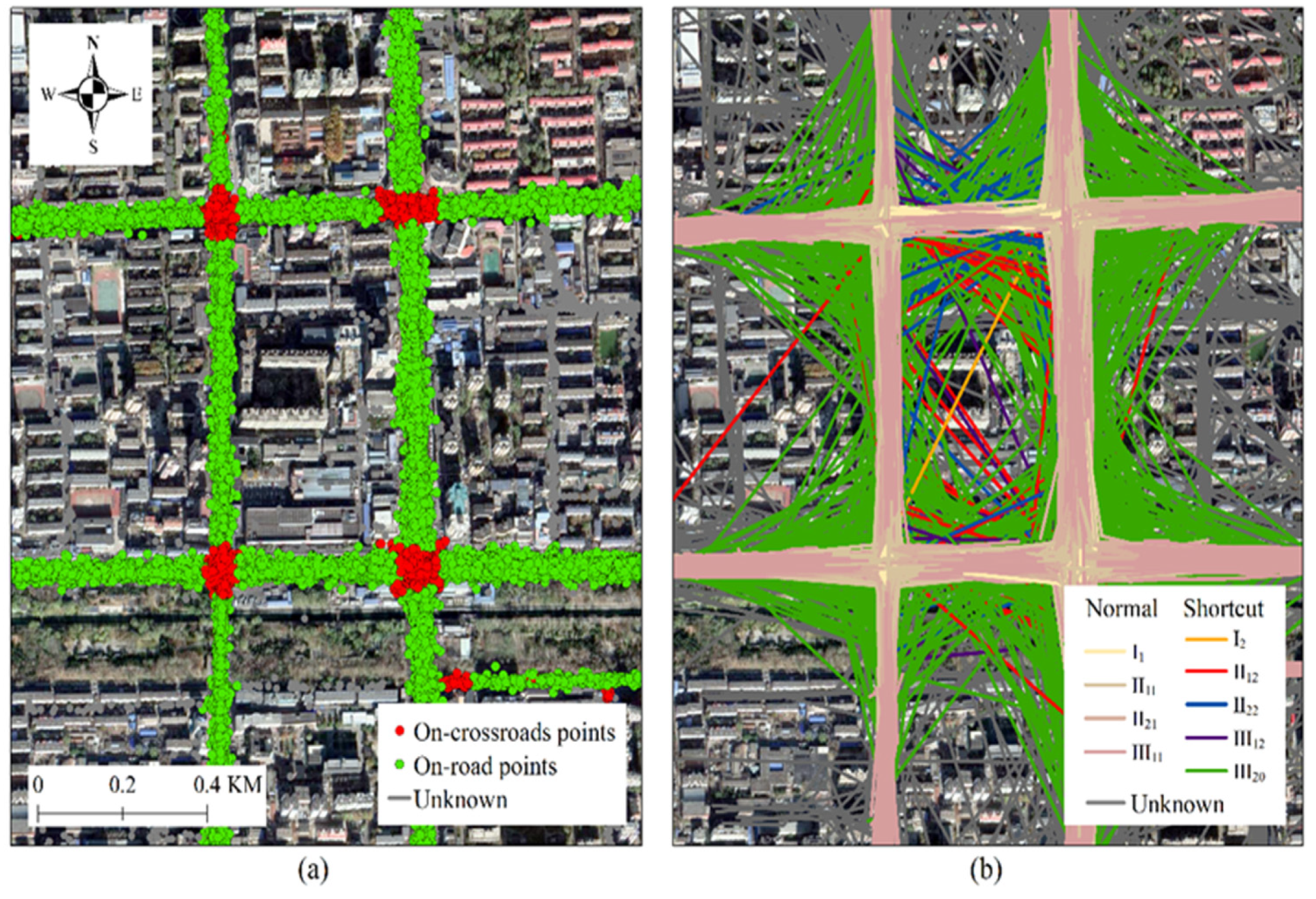
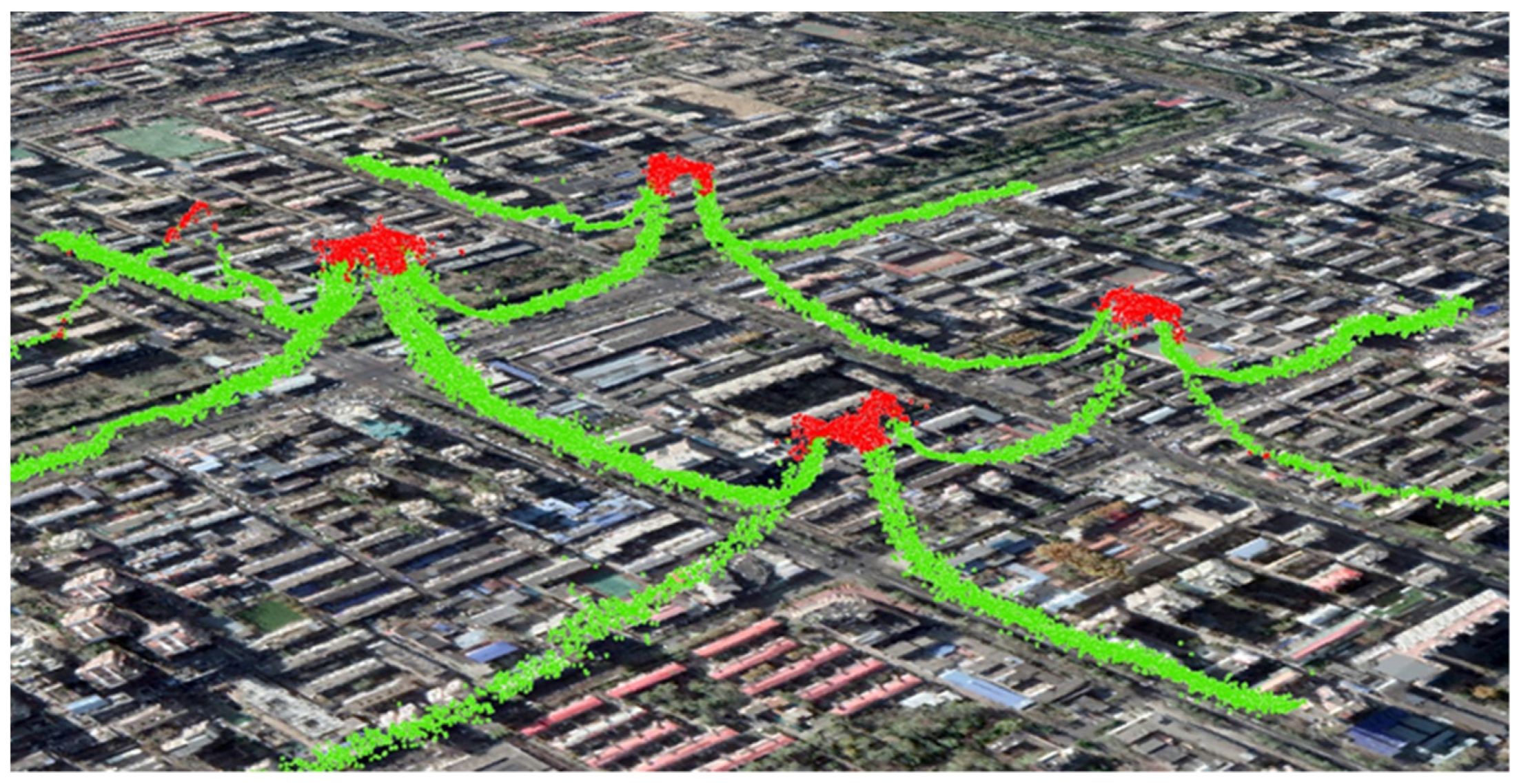
The endpoint type refers to the location of an endpoint, i.e., on the road or at a crossroads. An innovative endpoint-type determination algorithm is proposed in this study to divide the tracking points into two types (“on-road” vs. “on-crossroads”);

(3)

The “on-site” heading of a tracking point denotes the true moving direction of a vehicle in a road network. This is estimated using the number of nearby tracking link directions, without requiring ancillary datasets (e.g., road networks);

(4)

Link direction is the link heading that can be easily calculated using the coordinates and timestamps of two endpoints. In a shortcut link case, this direction is actually not the headings of vehicles;

(5)

The fractile line density of a link is the spatial density of tracking links that lie within a search window centered at a fractile position along the processed tracking link. For a shortcut link, two ending points are sitting on road-network, while most fractile points depart from roads. By default, we calculated three density values, i.e., at the start-, middle-, and end-points of the link.

2.2.2. Determining the Location of Tracking Points in the Road Network without Utilizing Ancillary Road Databases

To detect whether a tracking point is located on the road or at a crossroads, we need to analyze the spatial relationship between the tracking point and the intersection coverage. However, existing road network datasets (e.g., OpenStreetMap) are organized in the form of line features. Extracting intersections from a large scale street network map not only requires extra works but also faces some new technical problems such as how to determine the coverage of intersections. Therefore, an alternative solution that calculates advanced information entropy- and density- based geometric features only based on a trajectory dataset was developed to distinguish the type (“on-road” or “on-crossroads”) of tracking points in this work.

(1)

Measuring the information entropy at a tracking point

Tracking links on roads often have two major directions, which are opposite to each other, and tracking links within a crossroad area are usually omnidirectional. Given a tracking point, an information entropy metric is proposed to quantify the distribution of the directions of links near the point.

For each tracking point on a trajectory, we defined a search window with the size of the road width (e.g., 20 m) to extract tracking links that intersect with the window based on our experience. Based on the distribution of the directions of these links, we calculated the information entropy at the tracking point as follows.

We considered that $D=\left\{{\alpha }_1,{\alpha }_2,\dots ,{\alpha }_i,\dots ,{\alpha }_m\right\},{\alpha }_i\in \left[0,2\pi \right]$ is the collection of the direction values for the selected links that intersect with a window centered at the processed tracking point. We equally divided a circle centered at this tracking point into eight angle sectors and calculated the frequency distribution of the directions of these links, F $=\left\{f_1,\dots ,f_i,\dots ,f_8\right\}$. Subsequently, the information entropy, H, was calculated as follows:

$$H=-{{\displaystyle \sum }}_{j=1}^n{P}_j\log \left(P_j\right)$$

(1)

$$P_j=\frac{f_j}{{{\displaystyle \sum }}_{j=1}^n{f}_j}$$

(2)

where $f_j$ represents the number of links with directions lying within the jth angle sector; ${{\displaystyle \sum }}_{j=1}^n{f}_j$ is the total number of links in the window; $P_j$ is the probability. The sector number, $n$, was set to 8 by default.

Information entropy can be used to measure the complexity of a system. The more states the system has, the more information it possesses, the higher the entropy [39]. Based on Equation (1), the headings-based information entropy of tracking points on roads should be significantly lower than that of intersections. While there are mainly two opposite directions on a two-way road and one on a one-way road, there are more directions at an intersection to which several roadways with different directions often connect.

(2)

Measuring the line density gradient at a tracking point

The line density at a tracking point is the density of line features in the neighborhood of the processed tracking point, which is calculated in a magnitude-per-unit area from polyline features that fall within a radius around each cell. We note that the line density of an on-crossroads point is larger than that of an on-road point in most cases because crossroads have a larger traffic flow than connected roadways. Therefore, we proposed a line density gradient indicator to describe the difference between the line densities of on-crossroads and on-road points.

For a given tracking point, a filter kernel was defined using a three-by-three cell window. First, a specific cell centered at the point was defined and the eight nearest neighbors were aligned to the present cell. For each cell, we calculated the mean line density of the tracking points that it contains. The line density gradient was then calculated as follows:

$$G=[d_c-\max (d_i\left)\right]/d_c$$

(3)

where $G$ is the line density gradient at a tracking point, $d_c$ is the average line density of the center cell, and $d_i$ is the average line density of neighbor cell $i$, $i=1\dots 8$. In general, the gradient is a positive number at an intersection, fluctuates narrowly around zero on a roadway, and becomes negative in the transition area between the intersection and roadway.

(3)

Labeling tracking points by logistic regression

Logistic regression was adopted to judge whether a tracking point is “on-road” or “on-crossroads” based on information entropy and a line density gradient. The predictive statistics involve probabilistic nonlinear regression. Let $x=\left(x_1,x_2,\cdots ,x_n\right)$ be a vector with $n$ variables, and $\mathrm{P}\left(Y=1|x\right)$ be the probability of a tracking point being “on-crossroads” given its attribute values represented as an input vector x. The logistic regression model can be expressed as follows:

$$\mathrm{P}\left(Y=1|x\right)=\pi \left(x\right)=\frac{1}{1+e^{-g\left(x\right)}}$$

(4)

where $g\left(x\right)={\beta }_0+{\beta }_1{x}_1+\cdots +{\beta }_n{x}_n$, ${\beta }_0$ is the intercept, and $\beta =\left({\beta }_1,{\beta }_2,\cdots ,{\beta }_n\right)$ represents the regression coefficients of the explanatory variables that must be calibrated with the training samples. The range of $x$ was set to $\left[0,1\right]$ and the probability of the occurrence of the dependent variable $Y=1$ was estimated.

The maximum likelihood function was used to estimate $\beta$. Let $\left\{y_1,\cdots ,y_i,\cdots ,y_m\right\}$ be m observations from training samples and $y_i=0$denote that the ith sample is of an “on-road” type, whereas $y_i=1$ represents “on-crossroads”. The likelihood function of $m$ observations can then be expressed as:

$$\mathrm{L}\left(\beta \right)={\displaystyle \prod }_{i=1}^{m}p\left(y_i\right)={\displaystyle \prod }_{i=1}^{m}p{\left(x\right)}^{y_i}{\left[1-p\left(x\right)\right]}^{1-y_i}$$

(5)

By applying natural logarithms on both sides of Equation (4), a logarithmic likelihood function can be obtained, which can be used to solve the $\beta$ coefficients:

$$\ln L={\displaystyle \sum }_{i=1}^m\left[y_i\left({\beta }_0+{\beta }_1{x}_{i1}+\cdots +{\beta }_n{x}_{in}\right)-\ln \left(1+e^{{\beta }_0+{\beta }_1{x}_{i1}+\cdots +{\beta }_n{x}_{in}}\right)\right]$$

(6)

where$m$ is the number of observations and $n$ is the number of variables. The$\beta$ coefficients were estimated by maximizing $\ln L$ in an iterative process based on the commonly used Newton–Raphson method.

2.2.3. Estimating “On-Site” Headings at Two Endpoints of a Link

The “on-site” headings at the endpoints of a tracking link are the directions of vehicle moving forward. However, we did not use headings in our datasets in this study to guarantee our method enabled on those data sources that lack of vehicle heading measures; rather, we estimated the on-site heading based on the geostatistics of the tracking links that intersect with a search window centered at the endpoint. It is also possible to use the street network to estimate as vehicle heading is always identical to a roadway direction. The on-site heading is null if the endpoints are located within an intersection area.

Given an “on-road” point that is attached to a specific tracking link with a direction of ${\alpha }_{link}$, $D=\left\{{\alpha }_1,{\alpha }_2,\dots ,{\alpha }_i,\dots ,{\alpha }_m\right\},{\alpha }_i\in \left[0,2\pi \right]$ is the collection of directions of a total of m links that lie within a search window centered at the point. The cosine similarity function was used as a metric to measure how similar the directions of the two links are, as follows:

$$s_i=\cos (|{\alpha }_i-{\alpha }_{link}|), i\in \left[1,\mathrm{m}\right]$$

(7)

where a positive cosine value, $s_i$, represents the same moving direction (an intercross with an acute angle) and a negative value denotes an opposite direction (an intercross with an obtuse angle). Consequently, the m links in the search window can be separated into two groups.

We used the average of the directions of each group to approximate the roadway direction. The average direction with a positive cosine similarity is the on-site heading estimated at the processed endpoint. The on-site headings of two endpoints of a tracking link are represented as ${\beta }_i,i=0 \mathrm{or} 1$. We note that “on-site” headings of the “on-crossroads” endpoints were not calculated.

2.2.4. Calculation of the Line Density at a Fractile Position of a Tracking Link

The line density is the density of line features in a search window and was calculated in units of length per unit of area. Given a search window with a size d, the total number of $N$ tracking links was selected, where $l_i$ denotes the length of the ith link. The line density at the center of the window can be calculated as follows:

$$\rho =\frac{{{\displaystyle \sum }}_{i=1}^N{l}_i}{d^2}$$

(8)

Based on the assumption that $Q=\left\{q_1,\dots ,q_i,\dots ,q_m\right\}$ is the number of fractile points along a tracking link, $q_i$ is the ith fractile point on the link while $q_1$ and $q_m$ are the start- and end-points of the segment, respectively. The parameter $P=\left\{{\rho }_1,\dots ,{\rho }_i\dots ,{\rho }_m\right\}$ is the fractile line density at point $Q$ along the tracking link, which is calculated using Equation (8). Along a tracking link, an infinite number of fractile point can be set in theory. Two endpoints and at least one fractile point are required by our model. To reduce the large amount of calculation, we used $m=3$, in which the fractile point was the intermediate point of the link since the line density at this point is lower than others with a large probability.

2.3. Shortcut Tracking Link Detection Algorithm

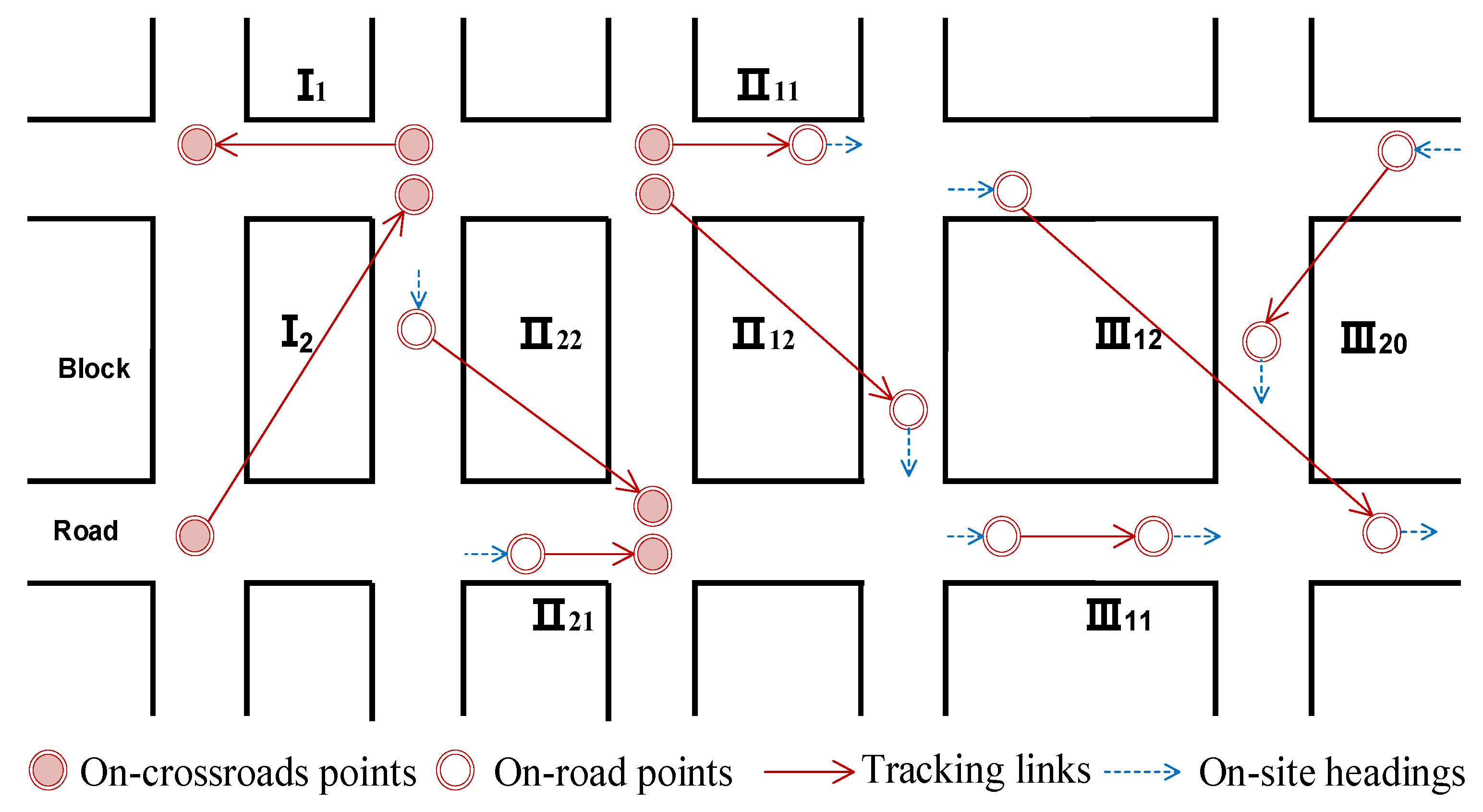
2.3.1. Spatial Patterns of Tracking Links

A tracking link may depict various spatial patterns in urban street grids. Based on the permutation and combination of the locations of two endpoints in the road network, tracking links can be grouped into three major spatial patterns: (I) both endpoints located at the crossroads, (II) one endpoint at the crossroads and the other on the road, and (III) both endpoints on roads.

By considering possible combinations of the link direction, on-site heading of endpoints, and fractile line densities, the three major groups can be further divided into several subgroups. The elementary spatial patterns of the tracking links after removing duplicates due to rotation, mirroring, and flipping are shown in Figure 3 in comparison to a street map which was partitioned into a road area and block area (representing the non-road area).

According to the Dimensionally Extended 9-Intersection Model (DE9M) (Egenhofer and Herring 1990), there are two types of spatial relationships between a tracking link and partitioned street map, i.e., the link may be completely within a road area or intersect with a block area. The former is called a normal link (I₁, II₁₁, II₂₁, and III₁₁), i.e., a straightforward link along a roadway, which overlaps with the vehicle ground truth path. The latter is called a shortcut outlier link (I₂, II₁₂, II₂₂, III₁₂, and III₂₀), which is a vehicle turning path without tracking points at the crossroads.

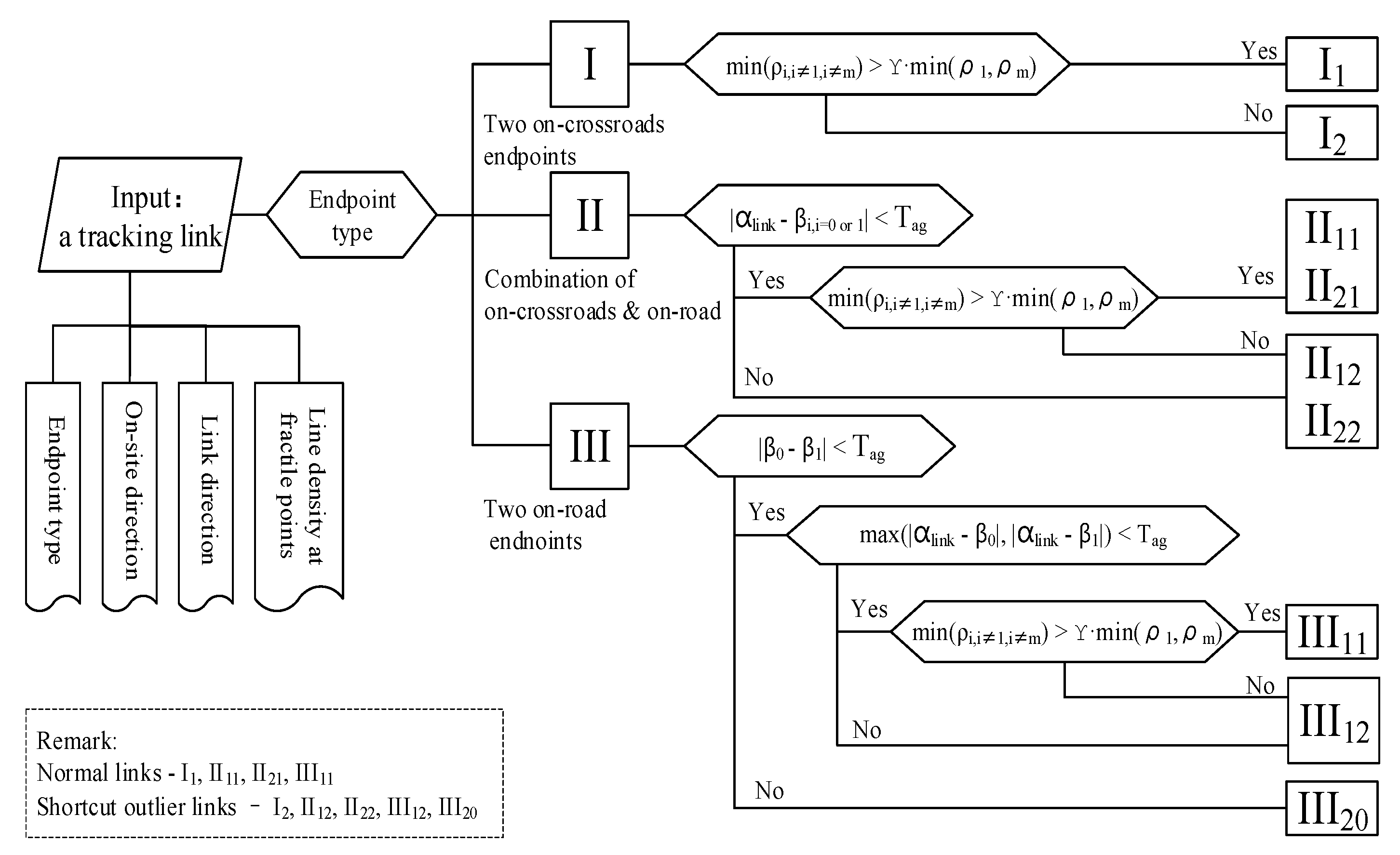
2.3.2. Detecting Shortcut Outliers by Spatial Reasoning

Whether a tracking link is normal or abnormal depends on whether the two endpoints of the link are on the same roadway. Considering that urban roads are straight or the path directions sharply change over a given distance of the tracking link with a reasonable length, we can define three criteria to infer whether a tracking link is a shortcut outlier based on the link’s geometric and motion measures:

The combination of two endpoints of the link based on point types;

The agreement between link direction and on-site headings of two endpoints;

The agreement among fractile line densities of the link.

Figure 4 illustrates the detection of link outliers (or spatial patterns) via spatial reasoning. The challenge is to decide if a tracking link may be deemed as normal or a shortcut.

If a tracking link fits the roadway well, the link direction must be close to the on-site headings of the two endpoints and all fractile line densities of the link must also be close to the densities at the two endpoints. Therefore, two fundamental coefficients, i.e., $T_{ag}$ for the direction similarity and $\gamma$ for the fractile line density similarity, were defined. The ranges of the two coefficients are discussed in the discussion section. Their default values (21° and 0.64, respectively) were estimated from the geostatistics of our subjective sampling design experiments.

3. Results

3.1. Study Area and Dataset

The trajectory dataset used in our experiments was based on the GNSS data from taxis in the urban area of Beijing, China, including 12,000 trajectories collected on 1 November 2012. The average distance between two consecutive tracking points is ~219 m and the sampling time intervals range from 12 to 65 s (Figure 5). This dataset is representative of low sampling rate trajectory databases acquired in big cities, which contain various noises and often cause the difficulty of path inference, map matching, or traffic rule extraction.

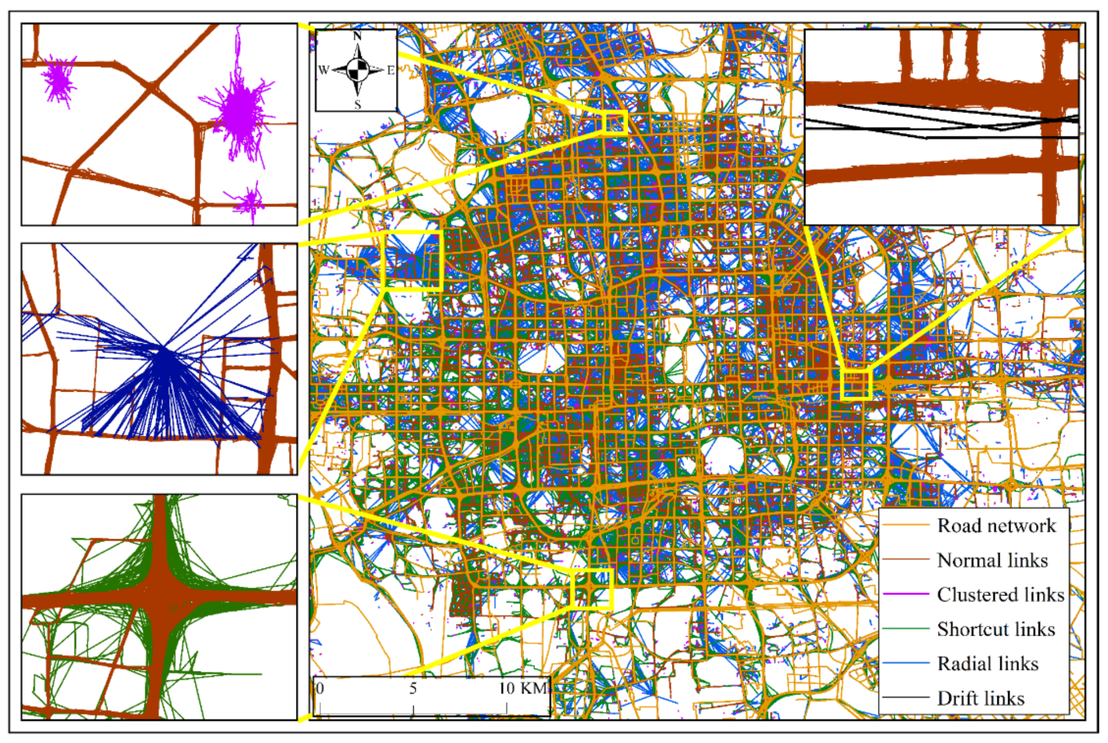
3.2. General Information on Detected Link Outliers

Without utilizing auxiliary databases (e.g., road networks), we first preprocessed the taxi trajectory datasets to identify radial, drift, and clustered link outliers. The dedicated shortcut detection method was then applied to determine implicit outliers using the spatial reasoning approach. As listed in

Table 1. Tracking link statistics.

Link Outliers				Normal Links	Total
Radial	Drift	Clustered	Shortcut
1,285,827	203,891	8,925,152	2,147,429	20,323,301	32,885,600
3.91%	0.62%	27.14%	6.53%	61.80%	100%

, poor tracking links account for ~38.2% of the entire test dataset; explicit outliers account for 4.5%; implicit outliers account for 33.7%. Most of the link outliers are clustered links, followed by shortcut links.

The tracking links were labeled and plotted on a map (Figure 6). The map shows that normal links reflect the straightforward grids of the street network. Clustered links mostly appear at crossroads, with some at roadside hot spots or parking lots. The patterns of the shortcut, radical, and drift links, which notably deviate from roads and overlap with residential blocks, are disorganized, such that street grids cannot be distinguished from these links.

Among all the link outliers, both clustered and shortcut links are signals. The former refers to vehicle short-time parking or stopping sites while the latter indicates road-intersections. Radial and drift links represent noise; however, they may be used to analyze the geo-context based on which the noise was generated.

3.3. Detailed Illustration of Shortcut Link Outliers

We selected the Mudanyuan district to determine the spatial characteristics of the shortcut link outliers. The roads (seville orange color) on the map (Figure 7) are district distributors that conduct the traffic among various residential, industrial, and principal business districts.

Among the tracking links within the Mudanyuan area, shortcut link outliers account for ~5.839% (

Table 2. Tracking link statistics for Mudanyuan.

Link Type	Count	(%)	Remarks
I1	8351	3.436	Normal
I2	1	0.004	Shortcut
II11	2442	10.049	Normal
II12	50	0.206	Shortcut
II21	2321	9.551	Normal
II22	50	0.206	Shortcut
III11	17,283	71.123	Normal
III12	13	0.053	Shortcut
III20	1305	5.370	Shortcut
Unknown	1008	4.148	Sparse or near boundary

). We note that the number of link outliers (III) is higher than that of the other outliers (I, II) because “on-road” links represent the majority in comparison with the “on-crossroads” links.

Based on overlapping all the tracking datasets, road networks, and Google images in this district (Figure 7), all of the preprocessed tracking points are high-quality points, which fluctuate within a narrow range around the streets and crossroads. Figure 7 shows that on-crossroads and on-road tracking points are well separated in space (Figure 7a).

However, the trajectory lines based on the connection of these consecutive points with tracking links present a complex intercross pattern (Figure 7b). All normal links together present a clear street grid. In contrast, the shortcut link outliers, which are actually simplified vehicle turning paths, are distributed in an unorganized manner near the crossroads. Advanced mining algorithms for these shortcut links could be utilized to recognize road intersections or traffic rules.

4. Discussion

4.1. Does the Information Entropy Effectively Describe the Separation of the Location of Tracking Points in a Road Network?

The tracking points were grouped into two categories (“on-crossroads” and “on-road”) based on the spatial relationship between the tracking points and road network without using the road network database. An information entropy descriptor was used to determine the difference between the two types of points.

Based on Equation (1), the information entropy for all tracking points in the Mudanyuan district was calculated. As illustrated in Figure 8, the information entropy values of the “on-crossroads” tracking points are significantly higher than those of the “on-road” tracking points. The farther a tracking point is from road intersections, the lower its information entropy is.

We interactively selected 11,368 sample tracking points at the inner side of the Second Ring Road of Beijing, among which 8556 are on the streets and 2812 are at intersections. Based on Equation (1), the information entropies were computed for all samples. In a handout test, these samples were divided into two folders, with one folder containing 9094 samples to train the logistic regression model and the other consisting of 2274 samples for validation.

K-fold cross-validation was used to test the parameters tuning and the performance of the trained logistic regression model. The 11,368 sample tracking points are divided into five folds, out of which four folds are for training and one is for testing. The results of five repeated classifications are shown in

Table 3. Accuracy of the tracking points classification.

		“On-Road”	“On-Crossroads”	Recall (%)	Kappa
Test 1	“on-road”	1679	8	99.53	98.63
	“on-crossroads”	4	583	99.32
	Precision (%)	99.76	98.65	-
Test 2	“on-road”	1685	10	99.41	98.50
	“on-crossroads”	3	576	99.48
	Precision (%)	99.76	98.29	-
Test 3	“on-road”	1714	10	99.41	98.21
	“on-crossroads”	5	545	99.09
	Precision (%)	99.71	98.20	-
Test 4	“on-road”	1704	15	99.13	97.63
	“on-crossroads”	5	550	99.10
	Precision (%)	99.71	97.35	-
Test 5	“on-road”	1691	14	99.18	97.55
	“on-crossroads”	7	562	98.77
	Precision (%)	99.59	97.57	-

. High Kappa scores from 97.55 to 98.72 were achieved based on the confusion matrix of the validation samples (Table 3), which implies a good level of agreement for the logistic regression used to distinguish the tracking points at road intersections from those on roads using the information entropy descriptor and line density gradient. The application of this logistic regression classifier to all tracking points of the test datasets shows that the “on-crossroads” points account for 24.70% of all the tracking points.

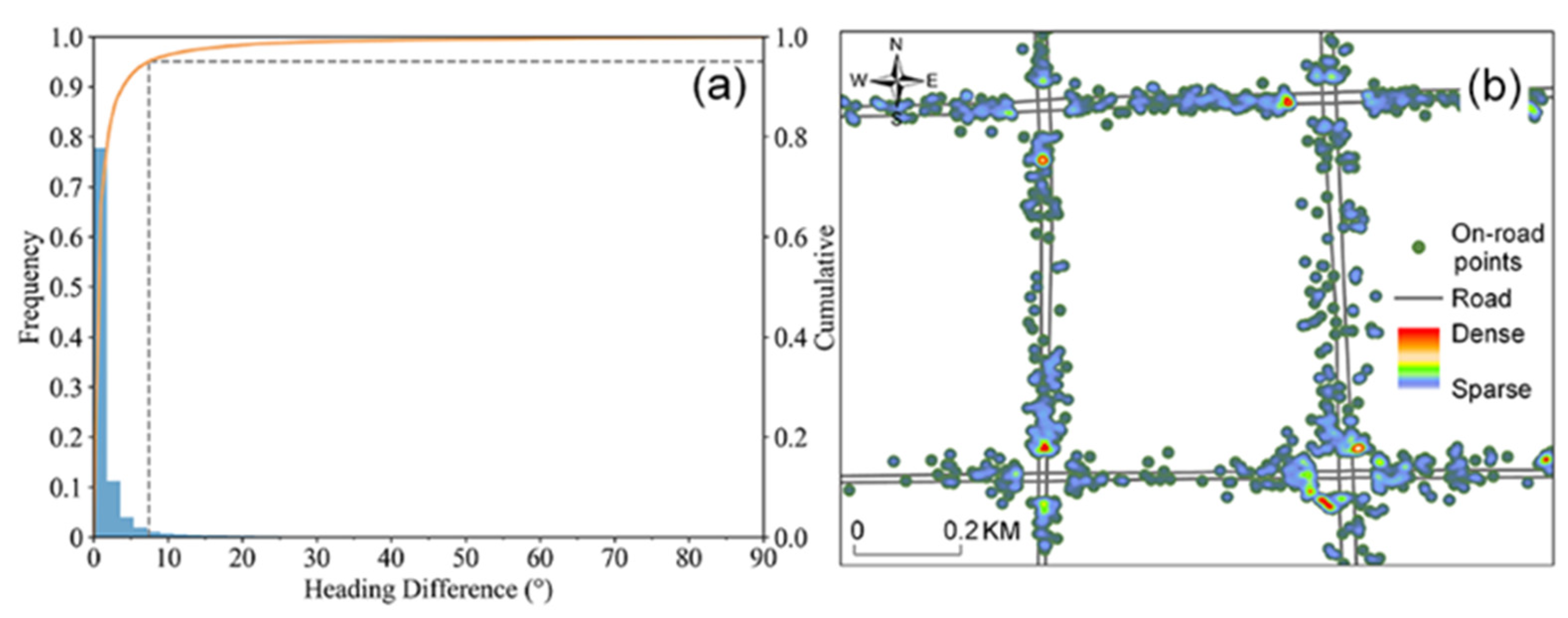
4.2. Can the On-Site Heading Be a Replacement for a Vehicle Heading on a Roadway?

For the tracking link of a vehicle, the estimated “on-site” heading at its endpoints is theoretically equivalent to the direction of the roadway on which the vehicle moves forward, but it actually has some difference. To evaluate the accuracy of the estimated on-site headings, the following test was performed in the Mudanyuan area: (1) there were four intersections in this area, each with four roadways (two directions of entering or exiting the intersection), so the ground truth headings of 25,026 on-road points were assigned to one of the lane directions according to their location, (2) the absolute errors or heading differences between the estimated headings and ground truth were calculated, and (3) the heading difference was illustrated based on statistics.

Based on the statistics, the average of the heading differences is 2.2° and the standard deviation is 6.58°, indicating that the on-site headings are close to the roadway direction. The density distribution of the heading differences represents a power-law distribution and the 95th percentile on the accumulative curve is ~7° (Figure 9a), which confirms the high accuracy of this method in terms of the estimation of on-site headings. This result shows that shortcut tracking links can be detected using estimated on-site headings other than the roadway directions from a road network auxiliary database.

To further explore the on-road points with large errors, 2281 on-road points with errors larger than 7° were selected to produce a heatmap (Figure 9b). The map shows that most of the inaccurate points were located near intersections because the omnidirectional presentation of the tracking links around an intersection affects the estimation of the directions of the connected roadways.

4.3. When Are On-Site Headings and Link Directions of the Same Link Considered Identical?

A tracking link must fit a roadway well if the direction of the link and on-site headings at two related endpoints are the same. However, due to the errors in estimating the on-site headings and calculating the link direction, they are not completely equal, despite the link that overlaps with the roadway. Therefore, an appropriate threshold ($T_{ag}$) is required. The directions and headings are the same if their difference is smaller than the threshold.

In a subjective sampling experiment, two groups of link samples were selected to test the differences among the link directions and on-site headings at two endpoints: normal (III₁₁) and shortcut (III₂₀) links. The measure of the difference between the on-site headings and link direction is defined as $\max \left(|{\alpha }_{link}-{\beta }_0\left|,|{\alpha }_{link}-{\beta }_1\right|\right)$.

For normal links, the indicator $\max \left(|{\alpha }_{link}-{\beta }_0\left|,|{\alpha }_{link}-{\beta }_1\right|\right)$ is mostly near zero and represents a hyperbola of a reciprocal function (Figure 10a1); this indicator is ~15° at the 95th percentile (Figure 10a2). For shortcut links, this indicator is ~24° at the 5th percentile (Figure 10b2), which contrasts with the theoretical value of 45°. In addition, the samples of two groups do not have the same distribution (p-value < 0.01 based on the Mann–Whitney U test).

Based on these results, we used an angle threshold range [15,24] for this indicator to separate the two cases and set the default to 20°. This value was set close to the threshold value (20°) to separate poor on-road points. The analyses of other link cases revealed similar results.

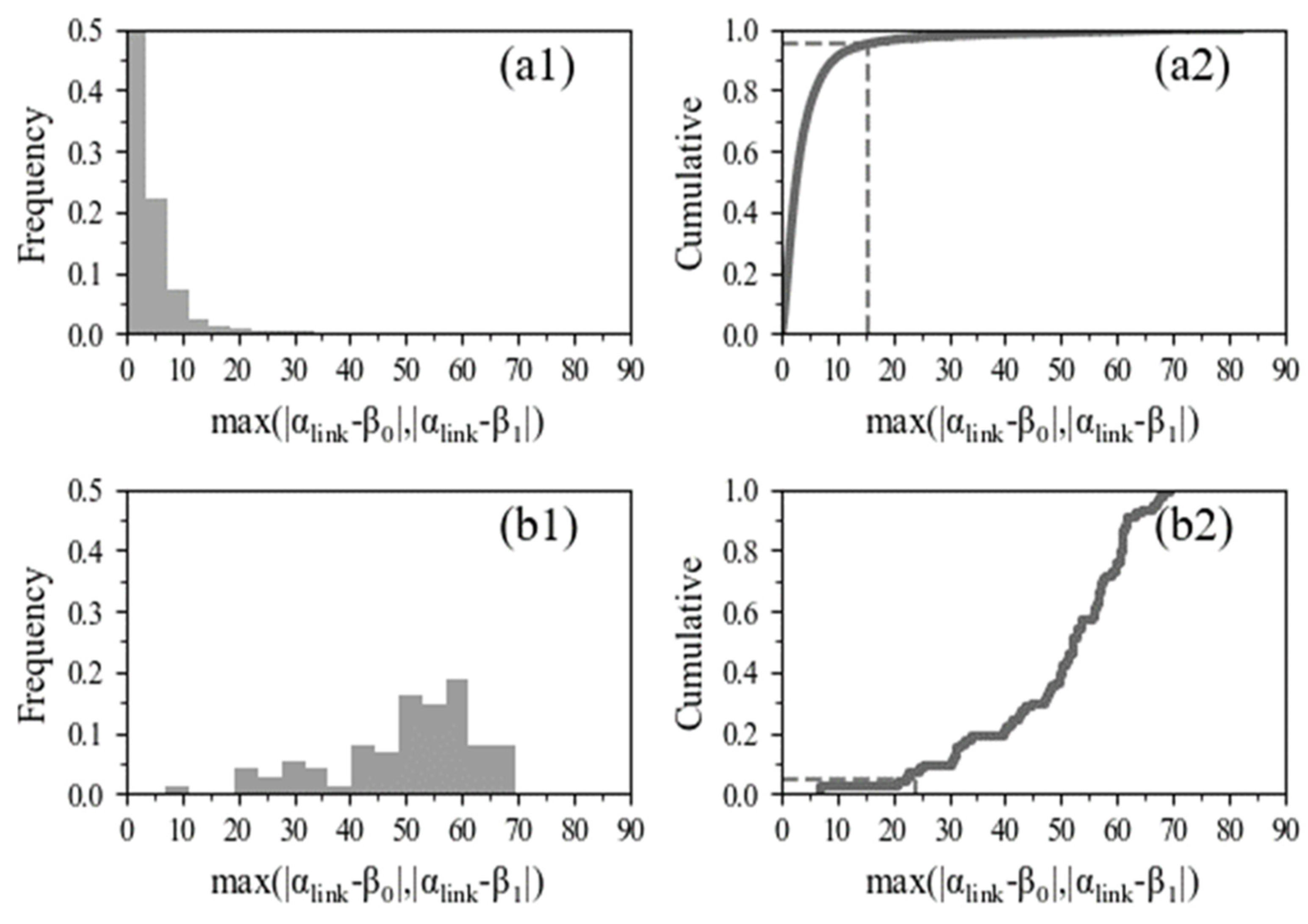
4.4. When Is the Change in the Fractile Line Densities along a Link Considered a Normal or Shortcut Link Case?

The line densities at all fractile positions of a normal tracking link distributed along a roadway should be similar. For a shortcut link with only two endpoints on a road network, the fractile line densities in the middle positions that taxis never reach should be significantly lower than at the two endpoints.

Based on Equation (8), an indicator, i.e., $\gamma =\min \left({\rho }_{i,i=1\dots m}\right)/\min \left({\rho }_1,{\rho }_m\right))$, was defined to describe the change in the fractile line densities along a link. In an ideal case, the indicator should be close to one for normal links and zero for shortcut links. Therefore, we can easily distinguish shortcut links from normal links.

Another sampling experiment was performed to determine the distribution of the $\gamma$ indicator values by reusing two sample groups. Based on the statistics of the fractile line densities, as illustrated in Figure 11(a1,b1), the $\gamma$ indicator yields significantly different distributions among normal links and shortcut links, as well as different histograms (p-value < 0.01 based on the Mann–Whitney U test). The 5th percentile for the normal links is 0.96 (Figure 11a2) and the 95th percentile for shortcut links is ~0.31 (Figure 11a2). Therefore, the $\gamma$ range was set to [0.31, 0.96] and the default was set to the average (0.64). The analyses of other link cases revealed similar results.

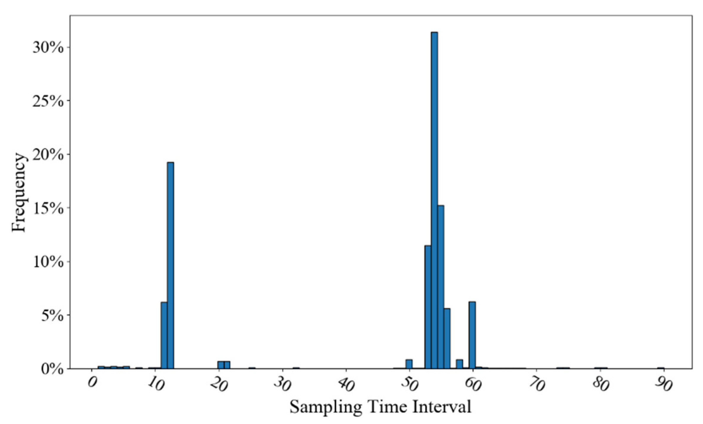
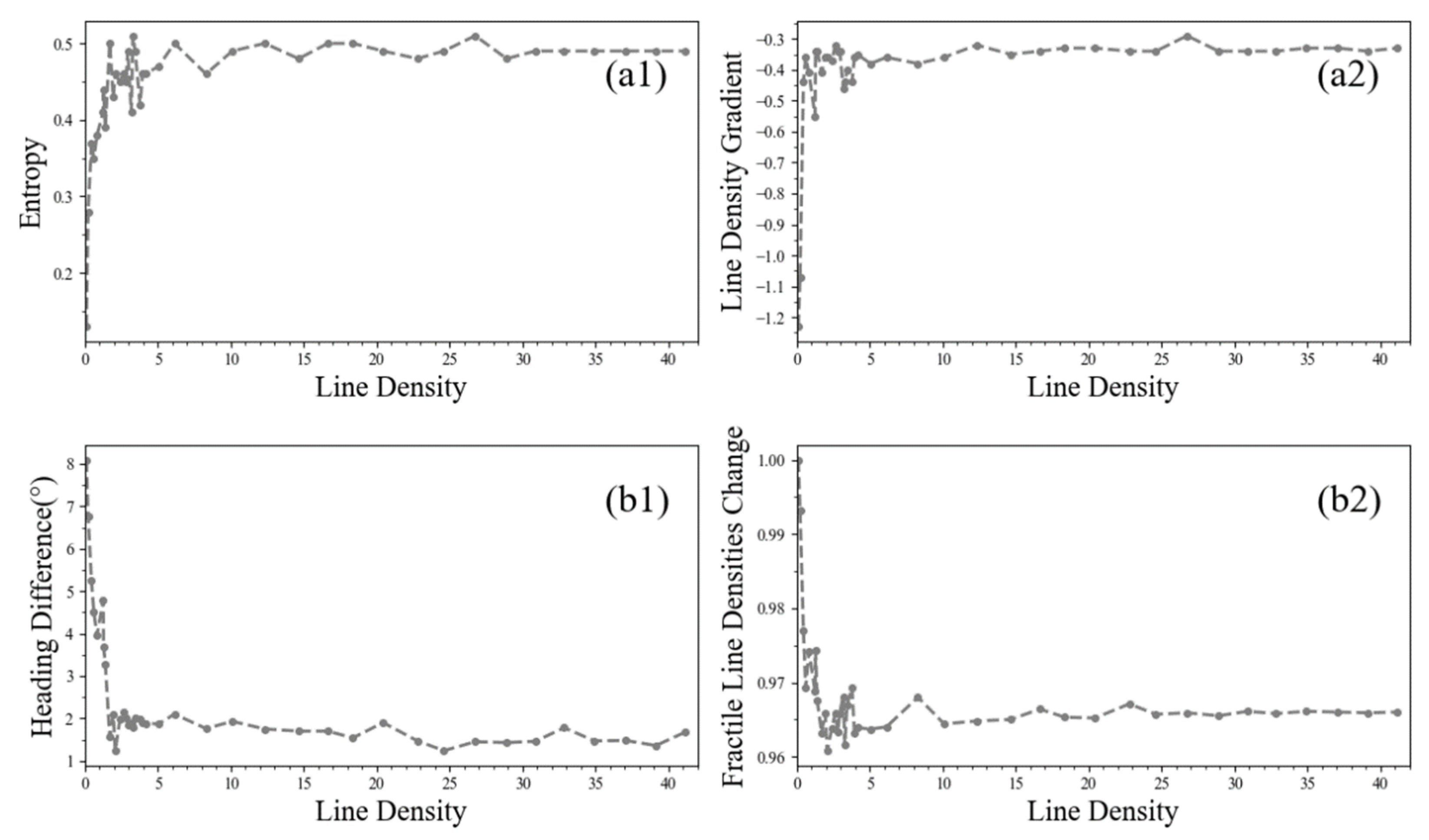
4.5. How Many Trajectories Are Necessary in Order to Make the Entropy- and Density-Based Approaches Work?

Based on our trajectory dataset at the Mudanyuan Intersection area, we randomly resampled into various sub-datasets with different line densities so that the effects of the sample’s line density on explainary variables in our approach can be illustrated. The sample size of these sub-datasets varied from 31 to 2873.

The entropy and line density gradient related to an intersection, which are together used to label tracking points, were first calculated on these subsets using a 35 m × 35 m window. As the sample’s line density gets larger, two variables’ value increases until they reach up to a limit at a line density of 5 (Figure 12(a1,b1)). Under this turning point, our approach may not satisfactorily classify tracking points. Another two parameters used in spatial reasoning, which are the difference between the on-site headings and link direction and the change in the fractile line densities along a link, were further calculated on the same sub-datasets. These two parameters change sharply on low line-density samples. Over the line density 4, they tend to converges progressively (Figure 12(b1,b2)). We took the maximal line-density in comparison of two turning points. If we count on the number of trajectories, about 407 vehicle traces are needed by our approach to achieve an acceptable output.

4.6. How Much Curvature of Urban Roads the Method Can Take without Leading to Errors?

There are also other situations where link shortcuts occur, e.g., along curvy roads. Therefore, we perform a robustness test to assess how much curvature (e.g., in terms of curvature radius) the method can take in an urban street network. A total of 27 concentric circles whose curvatures range from 0.001 m⁻¹ to 0.01 m⁻¹ were generated to simulate roads. Along each circle, 600 vehicle GNSS trajectories were simulated on which tracking points have positioning errors (0–15 m), time sampling interval (12–65 s), and speed (36.5 km/h).

The link shortcuts at intersections are identified if the “on-site” headings and the link direction are not identical. According to Section 4.3, for those non-shortcut links on straight roads, the measure of the difference between the on-site headings and link direction presents a power-law distribution ($X_1$). Therefore, we also calculate the same measures for the simulated links on each circle and obtain their distribution ($X_2$). If $X_2$ is stochastically larger than $X_1$, the curvature radius corresponding to $X_2$ will be taken as a threshold value to determine our method’s adoptability. The Mann–Whitney U test was used, in which the null and alternative hypotheses are $H_0:X_1<X_2$, $H_1:X_1\ge X_2.$As shown in

Table 4. Mann–Whitney U test for simulated curvy roads (or circles).

Curvature (m−1)	p-Value	Curvature (m−1)	p-Value	Curvature (m−1)	p-Value
0.001	0	0.0064	0.0055	0.0073	0.7638
0.002	0	0.0065	0.0060	0.0074	0.9993
0.003	0	0.0066	0.0100	0.0075	0.9964
0.004	0	0.0067	0.0177	0.0076	0.994
0.005	0	0.0068	0.0667	0.0077	0.9994
0.006	0	0.0069	0.0887	0.0078	1
0.0061	0	0.007	0.0939	0.0079	1
0.0062	0.0003	0.0071	0.3718	0.008	1
0.0063	0.0035	0.0072	0.5679	0.009	1

, the circles with curvature (<0.0068) and p-value (<0.0667) reject null hypotheses. Therefore curvy roads with a curvature radius great than 147 m can be processed by our method.

5. Conclusions

In this study, the GNSS vehicle trajectory was considered to be a set of tracking links. In addition to normal links, we defined four types of outliers (radial, drift, clustered, and shortcut) and proposed an integrated approach to detect these outliers. In particular, an advanced spatial reasoning method was developed to identify implicit shortcut outliers. This approach was tested using a taxi trajectory dataset for Beijing from 2012. The four types of outliers were successfully detected. The findings of this study can be summarized as follows:

• The proposed outlier detection method, which is based on a tracking link conceptual framework, can be used to process vehicle trajectory datasets without relying on road-network datasets. This is because the type of tracking points are determined by those density-and entropy-based features from trajectory dataset itself, and it can also be definitely recognized by matching open-access datasets i.e., OpenStreetMap.
• The shortcut link detection is based on spatial reasoning. A set of spatial patterns defining normal and shortcut links are identified and, correspondingly, several key geometric measures of a tracking link are proposed by understanding trajectory characteristics. Default threshold values of these measures are also determined by subjective sampling design and analysis.

Our research offers a new perspective for detecting outliers in trajectories, and yet there are some limitations. This approach is suitable for urban areas in which street grids are well presented, not curvy roads in mountainous regions, motorway intersections, or intersections on rural roads. Our approach, in which density, entropy, and even headings are based on statistics, is limited to the feature of line-density at intersections as discussed. In the future, we’d like to apply the model to more datasets that may reveal different patterns or irregularities of trajectories in space, and further improve the approach.

References

1. Liu, J.; Han, K.; Chen, X.; Ong, G.P. Spatial-temporal inference of urban traffic emissions based on taxi trajectories and multi-source urban data. Transp. Res. Part C Emerg. Technol. 2019, 106, 145–165. [Google Scholar] [CrossRef] [Green Version]
2. Yang, G.; Song, C.; Shu, H.; Zhang, J.; Pei, T.; Zhou, C. Assessing Patient bypass Behavior Using Taxi Trip Origin–Destination (OD) Data. ISPRS Int. J. Geo-Inf. 2016, 5, 157. [Google Scholar] [CrossRef] [Green Version]
3. Zhu, D.; Wang, N.; Wu, L.; Liu, Y. Street as a big geo-data assembly and analysis unit in urban studies: A case study using Beijing taxi data. Appl. Geogr. 2017, 86, 152–164. [Google Scholar] [CrossRef]
4. Guo, J.; Huang, W.; Williams, B.M. Real time traffic flow outlier detection using short-term traffic conditional variance prediction. Transp. Res. Part C Emerg. Technol. 2015, 50, 160–172. [Google Scholar] [CrossRef]
5. Lin, I.-C.; Cheng, C.-Y.; Lin, Y.-T. Improved location filtering using a context-aware approach. J. Ambient Intell. Smart Environ. 2021, 13, 1–18. [Google Scholar] [CrossRef]
6. Araki, M.; Kanamori, R.; Gong, L.; Morikawa, T. Impacts of Seasonal Factors on Travel Behavior: Basic Analysis of GPS Trajectory Data for 8 Months; Springer: Tokyo, Japan, 2017. [Google Scholar] [CrossRef]
7. Fu, Z.; Tian, Z.; Xu, Y.; Qiao, C. A Two-Step Clustering Approach to Extract Locations from Individual GPS Trajectory Data. ISPRS Int. J. Geo-Inf. 2016, 5, 166. [Google Scholar] [CrossRef]
8. Tanimoto, J.; Sagara, H. Social Diffusive Impact Analysis Based on Evolutionary Computations for a Novel Car Navigation System Sharing Individual Information in Urban Traffic Systems. J. Navig. 2011, 64, 711–725. [Google Scholar] [CrossRef]
9. Gong, S.; Cartlidge, J.; Bai, R.; Yue, Y.; Li, Q.; Qiu, G. Extracting activity patterns from taxi trajectory data: A two-layer framework using spatio-temporal clustering, Bayesian probability and Monte Carlo simulation. Int. J. Geogr. Inf. Sci. 2019, 34, 1210–1234. [Google Scholar] [CrossRef] [Green Version]
10. Zheng, Y. Trajectory Data Mining: An Overview. Acm Trans. Intell. Syst. Technol. 2015, 6, 1–41. [Google Scholar] [CrossRef]
11. Zheng, K.; Zheng, Y.; Xie, X.; Zhou, X. Reducing Uncertainty of Low-Sampling-Rate Trajectories. Proceedings of 2012 IEEE 28th International Conference on Data Engineering, Arlington, VA, USA, 1–5 April 2012; pp. 1144–1155. [Google Scholar]
12. Deng, M.; Huang, J.; Zhang, Y.; Liu, H.; Tang, L.; Tang, J.; Yang, X. Generating urban road intersection models from low-frequency GPS trajectory data. Int. J. Geogr. Inf. Sci. 2018, 32, 2337–2361. [Google Scholar] [CrossRef]
13. Ruan, S.; Long, C.; Bao, J.; Li, C.; Yu, Z.; Li, R.; Liang, Y.; He, T.; Zheng, Y. Learning to generate maps from trajectories. Proceedings of AAAI, Hilton New York Midtown, New York, NY, USA, 7–12 February 2020. [Google Scholar]
14. Djenouri, Y.; Belhadi, A.; Lin, J.C.-W.; Djenouri, D.; Cano, A. A Survey on Urban Traffic Anomalies Detection Algorithms. IEEE Access 2019, 7, 12192–12205. [Google Scholar] [CrossRef]
15. Knorr, E.M.; Ng, R.T.; Tucakov, V. Distance-based outliers: Algorithms and applications. VLDB J. 2000, 8, 237–253. [Google Scholar] [CrossRef]
16. Wang, J.; Rui, X.; Song, X.; Tan, X.; Wang, C.; Raghavan, V. A novel approach for generating routable road maps from vehicle GPS traces. Int. J. Geogr. Inf. Sci. 2015, 29, 69–91. [Google Scholar] [CrossRef]
17. Yan, Z.; Parent, C.; Spaccapietra, S.; Chakraborty, D. A Hybrid Model and Computing Platform for Spatio-semantic Trajectories. In The Semantic Web: Research and Applications, Proceedings of the 7th Extended Semantic Web Conference, ESWC 2010, Heraklion, Greece, 30 May–3 June 2010; Springer: Berlin/Heidelberg, Germany, 2010; pp. 60–75. [Google Scholar]
18. Wang, J.; Wang, C.; Song, X.; Raghavan, V. Automatic intersection and traffic rule detection by mining motor-vehicle GPS trajectories. Comput. Environ. Urban Syst. 2017, 64, 19–29. [Google Scholar] [CrossRef]
19. Zhao, S.; Li, W.; Cao, J. A user-adaptive algorithm for activity recognition based on k-means clustering, local outlier factor, and multivariate gaussian distribution. Sensors 2018, 18, 1850. [Google Scholar] [CrossRef] [Green Version]
20. Han, S.; Wang, J. Integrated GPS/INS navigation system with dual-rate Kalman Filter. GPS Solut. 2012, 16, 389–404. [Google Scholar] [CrossRef]
21. Vasiliev, K.; Saverkin, O. Comparative Evaluation of Algorithms for Trajectory Filtering. In Computer Vision in Control Systems; Springer: Cham, Switzerland, 2020; pp. 53–62. [Google Scholar] [CrossRef]
22. Maiz, C.S.; Molanes-Lopez, E.M.; Miguez, J.; Djuric, P.M. A Particle Filtering Scheme for Processing Time Series Corrupted by Outliers. IEEE Trans. Signal Process. 2012, 60, 4611–4627. [Google Scholar] [CrossRef]
23. Lee, J.-G.; Han, J.; Li, X.; Gonzalez, H. Traclass: Trajectory Classification Using Hierarchical Region-Based and Trajectory-Based Clustering. Proc. VLDB Endow. 2008, 1, 1081–1094. [Google Scholar] [CrossRef]
24. Liu, Z.; Pi, D.; Jiang, J. Density-based trajectory outlier detection algorithm. J. Syst. Eng. Electron. 2013, 24, 335–340. [Google Scholar] [CrossRef]
25. Yang, W.; Ai, T.; Lu, W. A Method for Extracting Road Boundary Information from Crowdsourcing Vehicle GPS Trajectories. Sensors 2018, 18, 1261. [Google Scholar] [CrossRef] [Green Version]
26. Hadjieleftheriou, M.; Kollios, G.; Tsotras, V.J.; Gunopulos, D. Efficient Indexing of Spatiotemporal Objects. In Proceedings of the 8th International Conference on Extending Database Technology: Advances in Database Technology, Prague, Czech Republic, 25–27 March 2002; Springer: Berlin/Heidelberg, Germany, 2002; pp. 251–268. [Google Scholar]
27. Mamoulis, N.; Cao, H.; Kollios, G.; Hadjieleftheriou, M.; Tao, Y.; Cheung, D. Mining, indexing, and querying historical spatiotemporal data. In Proceedings of the Tenth ACM SIGKDD International Conference on Knowledge Discovery and Data Mining, Seattle, WA, USA, 22–25 August 2004; Volume 236, pp. 236–245. [Google Scholar]
28. Hunter, T.; Abbeel, P.; Bayen, A. The Path Inference Filter: Model-Based Low-Latency Map Matching of Probe Vehicle Data. IEEE Trans. Intell. Transp. Syst. 2014, 15, 507–529. [Google Scholar] [CrossRef] [Green Version]
29. Rahmani, M.; Koutsopoulos, H.N. Path inference of low-frequency GPS probes for urban networks. In Proceedings of the 15th International IEEE Conference on Intelligent Transportation Systems, Anchorage, AK, USA, 16–19 September 2012. [Google Scholar]
30. Jenelius, E.; Koutsopoulos, H.N. Travel time estimation for urban road networks using low frequency probe vehicle data. Transp. Res. Part B Methodol. 2013, 53, 64–81. [Google Scholar] [CrossRef] [Green Version]
31. Meng, F.; Guan, Y.; Lv, S.; Wang, Z.; Xia, S. An overview on trajectory outlier detection. Artif. Intell. Rev. 2018. [Google Scholar] [CrossRef]
32. Guan, Y.; Xia, S.; Lei, Z.; Yong, Z.; Cheng, J. Trajectory Outlier Detection Algorithm Based on Structural Features. J. Comput. Inf. Syst. 2011, 7, 4137–4144. [Google Scholar]
33. Yang, X.; Tang, L.; Li, Q. Generating Lane-based Intersection Maps from Crowdsourcing Big Trace Data. Transp. Res. Part C Emerg. Technol. 2018, 89, 168–187. [Google Scholar] [CrossRef]
34. Binh, H.; Ling, L.; Omiecinski, E. Road-Network Aware Trajectory Clustering: Integrating Locality, Flow, and Density. IEEE Trans. Mob. Comput. 2015, 14, 416–429. [Google Scholar] [CrossRef] [Green Version]
35. Xu, Z.; Cui, G.; Zhong, M.; Wang, X. Anomalous Urban Mobility Pattern Detection Based on GPS Trajectories and POI Data. ISPRS Int. J. Geo-Inf. 2019, 8, 308. [Google Scholar] [CrossRef] [Green Version]
36. Hawkins, D.M. Identification of Outliers. Biometrics 1980, 37, 860. [Google Scholar] [CrossRef]
37. Liu, W.; Li, J.; Zeng, Q.; Guo, F.; Wu, R.; Zhang, X. An improved robust Kalman filtering strategy for GNSS kinematic positioning considering small cycle slips. Adv. Space Res. 2019, 63, 2724–2734. [Google Scholar] [CrossRef]
38. Xiang, L.; Gao, M.; Wu, T. Extracting Stops from Noisy Trajectories: A Sequence Oriented Clustering Approach. ISPRS Int. J. Geo-Inf. 2016, 5, 29. [Google Scholar] [CrossRef] [Green Version]
39. Wehrl, A. General properties of entropy. Rev. Mod. Phys. 1978, 50, 221–260. [Google Scholar] [CrossRef]
Figure 1. Four types of outlier tracking links (tracking points, tracking links, radial outliers, drift outliers, clustered outliers, and shortcut outliers are shown in (a), (b), (c), (d), (e), and (f), respectively).
Ijgi 10 00333 g001
Figure 2. An integrated approach for the detection of outlier tracking links.
Ijgi 10 00333 g002
Figure 3. Spatial patterns of the tracking links, with normal links, i.e., I1, II11, II21, and III11, and shortcut outlier links, i.e., I2, II12, II22, III12, and III20.
Ijgi 10 00333 g003
Figure 4. A schematic diagram showing the spatial reasoning workflow.
Ijgi 10 00333 g004
Figure 5. Sampling time intervals of the dataset.
Ijgi 10 00333 g005
Figure 6. Plot of the labelled tracking links in Beijing.
Ijgi 10 00333 g006
Figure 7. High-quality tracking points versus poor-quality tracking links at the Mudanyuan site: (a) shows that on-crossroads and on-road tracking points are well separated in space and (b) shows the complex intercross pattern of poor-quality tracking links at the intersection area.
Ijgi 10 00333 g007
Figure 8. Three-dimensional map of the information entropy values for the tracking points in the Mudanyuan area, where red represents the on-crossroad points and green is the on-road points.
Ijgi 10 00333 g008
Figure 9. Differences between on-site headings and roadway directions: (a) shows the histogram and cumulative curve of headings differences and (b) shows the spatial distribution of on-road points with errors larger than 7°.
Ijgi 10 00333 g009
Figure 10. Agreement between two directions, i.e., max ( | α l i n k β 0 | ,   | α l i n k β 1 | ) , is defined to measure the difference between the on-site headings and link direction. (a1) and (b1) respectively show the measured values of the normal and abnormal links and (a2) and (b2) for the cumulative curve, respectively.
Ijgi 10 00333 g010
Figure 11. Changes in the fractile line densities, i.e., min ( ρ i , i = 1 m ) / min ( ρ 1 , ρ m ) ) ,   is defined to describe the change in the fractile line densities along a link: (a1) and (b1), respectively, show the measured values of the normal and abnormal links and (a2) and (b2) for the cumulative curve, respectively.
Ijgi 10 00333 g011
Figure 12. Effects of sample size on four parameters: (a1) and (a2) are about the entropy and density gradient; (b1) and (b2) are related to on-site heading and fractile line-density.
Ijgi 10 00333 g012