A Dynamic and Static Context-Aware Attention Network for Trajectory Prediction

Abstract

Forecasting the motion of surrounding vehicles is necessary for an autonomous driving system applied in complex traffic. Trajectory prediction helps vehicles make more sensible decisions, which provides vehicles with foresight. However, traditional models consider the trajectory prediction as a simple sequence prediction task. The ignorance of inter-vehicle interaction and environment influence degrades these models in real-world datasets. To address this issue, we propose a novel Dynamic and Static Context-aware Attention Network named DSCAN in this paper. The DSCAN utilizes an attention mechanism to dynamically decide which surrounding vehicles are more important at the moment. We also equip the DSCAN with a constraint network to consider the static environment information. We conducted a series of experiments on a real-world dataset, and the experimental results demonstrated the effectiveness of our model. Moreover, the present study suggests that the attention mechanism and static constraints enhance the prediction results.

1. Introduction

Trajectory prediction is one of the core problems that need to be solved in autonomous driving. Human drivers often predict the trajectory of surrounding vehicles by observing the driving conditions of surrounding vehicles and road environments based on their own experience. However, autonomous vehicles, which are able to move without drivers, cannot follow this rule. Vehicles in motion encounter different road conditions and various dynamic traffic participants, which may pose potential threats to safe driving. In autonomous driving scenarios, perceiving the surrounding situation and predicting its trend are crucial abilities to ensure the safety of vehicles. Based on the collected data, trajectory prediction methods can help the system make more robust and stable decisions.

To achieve driving autonomously in complex traffic, it is necessary for vehicles to infer the future movement of surrounding vehicles. Compared with general dynamic problems, vehicle trajectory prediction usually occurs in an open random environment that increases the difficulty and complexity of modeling. On the one hand, the vehicle is subject to many constraints, such as road conditions and surrounding moving targets. On the other hand, affected by the driver’s driving intention and style [1], the trajectory tends to be highly nonlinear over time. These challenges have caused the degradation of both traditional dynamic models and machine learning models

Therefore, trajectory prediction methods based on deep learning have become a current research hotspot. Recurrent Neural Network (RNN), especially Long Short-Term Memory (LSTM) model, is widely favored for its excellent performance in time series data analysis. Some studies [2,3] show that the Sequence to Sequence (Encoder–Decoder) Network, which is commonly used in machine translation, has a good performance in multistep trajectory prediction scenarios. Increasing research emphasizes interaction-aware modeling, such as Convolutional Social LSTM (CS-LSTM) [4], proposed using Convolutional Neural Network (CNN) to model the motion state of surrounding vehicles to introduce multi-vehicle interaction factors to optimize trajectory prediction. Due to its high accuracy and feasibility, CS-LSTM has been widely concerned by scholars. However, CS-LSTM lacks consideration of interaction changes and environmental constraints. In this paper, we propose a dynamic and static context-aware attention network (DSCAN) for vehicle trajectory prediction. Our model uses the attention mechanism to model the inter-vehicle interaction information dynamically and uses feature embedding learning to strengthen the constraint effect of a static environment. In particular, our model can be characterized by the following:

(1) Attentional decoder: We use an attention-based LSTM to generate intermediate vectors at different prediction time steps to solve the problem that social pooling [5] leads to the same weight of surrounding vehicles. Our decoder can assign reasonable weights to surrouding vehicles and adaptively selects the most noteworthy vehicles at each time-step.

(2) Constraint net: We propose a shallow neural network, a constraint net, to extract and model surrounding environmental constraints. It has the advantages of convenient computation and high scalability. Combined with the representations of vehicles’ trajectories, it makes trajectory prediction results closer to the reality.

2. Literature Review

According to the motion of vehicles, trajectory prediction methods can generally be divided into four types: physical-based, maneuver-based, interaction-aware, and environment-aware methods.

Physics-based motion model: These models only take the vehicle’s control (e.g., steering and acceleration) and properties (e.g., weight) data [6]. The simplest models are the Constant Velocity (CV) and Constant Acceleration (CA) models [7,8]. References [9,10] used a normal distribution to handle the uncertainty on the vehicle state. Furthermore, Reference [11] used Monte Carlo simulation to remove the generated trajectories that exceed physical limits. These original models depend on a vehicle’s representation of the dynamics and kinematics, in which the results are up to the laws of physics. Therefore, they can only be applied to short-term (less than 1 s) vehicle trajectory prediction.

Maneuver-based motion model: They predict trajectory by recognizing in advance the maneuvers that drivers intend to perform. These methods assume that the motion of the vehicle matches its previous maneuver. Atev et al. [12] calculated the Hausdorff distance between two trajectories to measure their similarity. Based on Support Vector Machine (SVM) and Bayesian filtering, Kumar et al. [13] implemented online lane-change intention prediction. Qiao et al. [14] abstracted trajectory as a series of discrete motions and used Hidden Markov Model (HMM) to predict moving objects’ trajectories. Moreover, heuristic-based classifiers [15], random forest classifiers [16], and RNNs have been adopted for maneuver recognition. These methods are more advanced and reliable, but they still regard vehicles as independent entities and ignore vehicles’ impact.

Interaction-aware motion model: The research object and its surrounding vehicles are interactive motion entities. Compared with the previous two methods, these methods are more in line with the real traffic scenarios and more complex. Alahi et al. [5] proposed social pooling for pedestrian trajectory prediction in crowded public spaces. They meshed the space and preserved the spatial information through grid-based pooling. As a continuation, Deo et al. [4] proposed CS-LSTM. The authors used social pooling [5] for vehicle trajectory prediction and considered the impact of surrounding vehicles. Recent research [17] showed that besides behavior prediction, an important issue is to take inter-vehicle interaction into account. However, the social pooling methods resulted in the same impact weight for each entity around the research object. Thus, Xu et al. [18] proposed an exclusion equation to calculate the impact of pedestrians at different distances on the research object and weighted the historical trajectory encoding results accordingly. Generative Adversarial Networks (GANs) are also used in trajectory prediction. Reference [19] proposed Social-GAN with a generator composed of an LSTM-based encoder, context-pooling module, and an LSTM-based decoder. Its discriminator also used LSTMs. However, GANs have a flaw. They are challenging to achieve the Nash equilibrium, consuming much time.

Considering the interaction between vehicles, interaction-aware motion models are closer to the real driving scenario, and their prediction results are more reliable. A vehicle’s motion is affected by the surrounding vehicles on the road, and the impact constantly changes. Some existing models focus on vehicles’ track history to learn the surrounding dynamic information but ignore the impact of static environment constraints on the road. In terms of this issue, some studies began to concern road constraints.

Environment-aware model: These methods add environmental information to the models mentioned above, making the generalization ability stronger. The experiment in [20], which took lanes and signs into account, used the state consists of vehicle status and environment information. For each expert trajectory, they synthesized one trajectory based on the associated environment. Reference [21] realized a constrained MRN (Maneuver Recognition Network), in which the output of the GRU encoder was concatenated with the road’s structural constraints vector. However, these works only consider the specific environment structure or limited data types, which are difficult to extend.

Both dynamic and static context factors affect the final prediction accuracy and must be considered in driving.

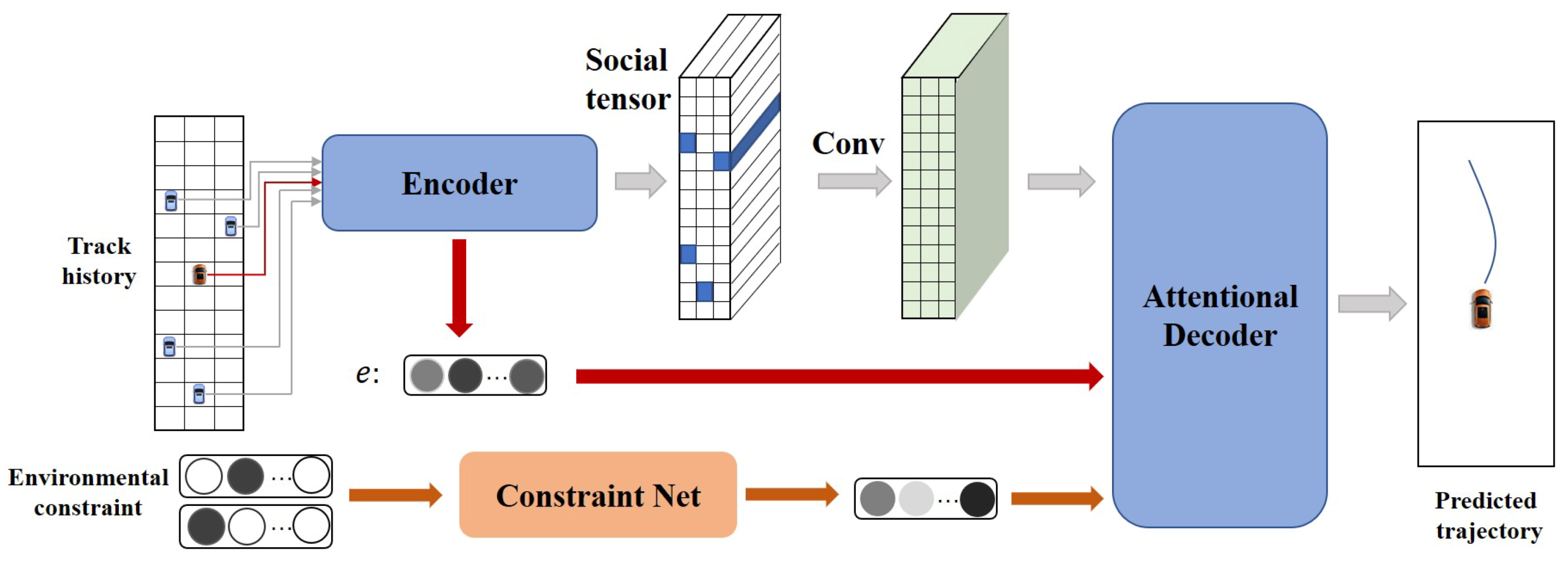
3. Methodology

A reliable driving trajectory should be generated by multiple factors such as surrounding vehicles and environment constraints. Therefore, a robust vehicle trajectory prediction model needs to take these factors into account. Figure 1 shows the architecture of our proposed model, DSCAN. It mainly consists of an LSTM encoder, a constraint net, and an attentional decoder. DSCAN takes vehicles’ historical trajectories and environmental constraints as input. The LSTM encoder and the constraint net, respectively, model them. Our proposed attentional decoder then concatenates the representations at the previous step to obtain the final trajectory prediction result.

3.1. Encoder

An LSTM is a neural network that accounts for dependencies across observations in a time series. It is controlled by three gates, of which the forget gate is the most important. The forget gate uses a decay rate $f_t$ to make the LSTM with long-term memory [22,23] and it depends on the previous output $h_{t-1}$ and current input $x_t$. This step can be expressed by Equation (1).

$$f_t=\sigma \left(W_f·\left[h_{t-1},x_t\right]+b_f\right)$$

(1)

As such, they are commonly used for forecasting purposes. We adopt LSTM as our encoder for its superior performance in time series problems. Since all historical trajectories obey the same data distribution, we encode the vehicles’ trajectories to accelerate network optimization, namely

$$e_i=LSTM\left(tra{j}_i\right),i\in \{0,1,2\dots ,m\},$$

(2)

where $e_i\in R^{d_{enc}}$ denotes the encoding representation of the $vehicl{e}_i$’s historical trajectory $tra{j}_i$. As shown in Figure 1, the LSTM encoder models the target vehicle historical trajectory

$$tra{j}_0=\left\{\left(x_1,y_1\right),\left(x_2,y_2\right),\dots ,\left(x_T,y_T\right)\right\}$$

(3)

and the surrounding vehicle historical trajectory $\left\{tra{j}_1,tra{j}_2,\dots ,tra{j}_m\right\}$ to learn the dynamics of vehicle motion.

As performed in [4], we also define an occupancy grid based on the lanes to set up our social tensor. Using this social tensor and the LSTM state of the vehicle, the prediction accuracy has been shown to improve [5,24]. Reference [4] pointed out that the convolutional layer can expand the grid receptive field and can enhance grid information fusion. We attach each surrounding vehicle’s representation $(e_i,i\in \left\{1,2,\dots ,m\right\})$ into a $3\times 13$ grid to preserve the spatial correlations and add a convolutional layer with the kernel of $3\times 3$. Since the convolutional neural network retains identity mapping, it also strengthens the model’s ability to learn and express. Finally, the encoder takes the target vehicle representation $e_0\in R^{d_{enc}}$ and its convolution-processed surrounding vehicles’ representations $C\in R^{3\times 13\times d_{conv}}$ as output for further decoding.

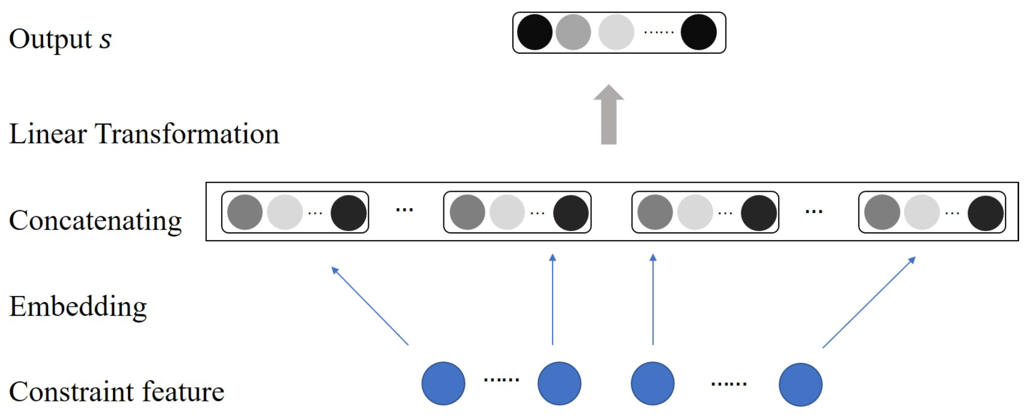
3.2. Constraint Net

Even if surrounding vehicles’ motion and driving intention are similar, the vehicle’s future trajectory may still be affected by environmental factors (such as lanes, weather, and traffic policies). For example, vehicles driving in the rain tend to move slowly and avoid overtaking [25,26]. Moreover, as the technology of V2I (Vehicle to Infrastructure) evolves [27,28], the infrastructure can provide more environmental information to the vehicle, which needs a network to process. Referring to Wide&Deep [29] and DeepFM [30], we propose a shallow neural network (Constraint Net) to model environmental constraints. As illustrated in Figure 2, we first collect and discretize raw environmental information into a group of category features (e.g., “sunny” as 0 and “rainy” as 1), then the proposed constraint net takes these extracted environmental features as input and calculate a concentrated representation as output.

Given a group of environmental features $\left[f_1,f_2,\dots ,f_I\right]$, where I is the number of feature fields, the embedding layer converts each of them to a dense continuous vector representation $\widetilde{f_i}$ with dimension $d_{conv}$. To achieve a dimension reduction, the constraint net applies a single-layer neural network upon the concentration of embedding vectors and outputs s with concentrated environmental information. This process can be expressed as follows:

$$s=W_{s}Leaky\underline{}ReLU\left(\left[{\tilde{f}}_1;{\tilde{f}}_2;\dots ,{\tilde{f}}_I\right]\right)+b_s,$$

(4)

where $s,b_s\in R^{d_{\mathrm{conv}}},W_s\in R^{d_{conv}\times (I·d_{conv})}$.

As discussed above, the constraint net is able to convert a variable number of features $\left[f_1,f_2,\dots ,f_I\right]$ into a fixed length vector s, which means it is convenient to introduce new environmental feature without modifying other network components of the complete model. Moreover, the computational complexity of the constraint net is $O\left(I{d}_{conv}^2\right)$. Compared with other components such as the LSTM encoder, the computational complexity of constraint net is negligible and grows linearly with the number of feature fields.

However, limited by the public dataset’s feature collection, we mainly extract lane-related environmental features in our experiment, including the following three aspects: the target vehicle’s lane, whether it is driving in the left or right lane. We leave the exploration of other environmental features as our future work. We also demonstrate the effectiveness of the constraint net in Section 4.

3.3. Attentional Decoder

We propose an attentional decoder that handles the information in the previous step to generate the predictive distribution for the future trajectory. Similar to the encoder, we use an LSTM network as the primary decoder to achieve multistep trajectory prediction. The attentional mechanism is widely used in series forecasting for its good performance, such as machine translation [31], image annotation [32], speech recognition [33], text summarization [34], and trajectory prediction [35]. For efficiently solving the high-dimensional encoding representation C and dynamically paying attention to surrounding vehicles’ motion, we also apply the attention mechanism to the decoder so that our decoder can adaptively select the most noteworthy surrounding vehicles at each time-step.

Precisely, according to the previous hidden state $h_{t-1}$, the decoder computes the attention weight of each grid $C_{i,j}\in R^{d_{conv}}$ in C at time step t and then weight them (as shown in Equations (5)–(7)):

$$\begin{array}{cc}\hfill scor{e}_{i,j}^t& =v^{T}tanh\left(W_h{h}_{t-1}+W_c{C}_{i,j}\right),\hfill \end{array}$$

(5)

$$\begin{array}{cc}\hfill {\alpha }_{i,j}^t& =\frac{exp\left(scor{e}_{i,j}^t\right)}{{\sum }_{p,q}exp\left(scor{e}_{p,q}^t\right)},\hfill \end{array}$$

(6)

$$\begin{array}{cc}\hfill \widetilde{C^t}& =\sum _{i,j}{\alpha }_{i,j}^t{C}_{i,j},\hfill \end{array}$$

(7)

where $i\in \left\{1,2,3\right\},j\in \left\{1,2,\dots ,13\right\}$ are grid coordinates and $\widetilde{C^t}\in R^{d_{conv}}$ is weighted attention representation. $scor{e}_{i,j}^t$ and ${\alpha }_{i,j}^t$ are the intermediate variable and attention weight for $C_{i,j}$ at time step t, respectively.

After computing the attention distribution and concatenating it with the representations of the target vehicle and constraints $\left(\left[e_0,\widetilde{C^t},s\right]\right)$, the decoder takes them as input and deduces this high-dimensional tensor at this time step. Finally, it generates the future trajectory prediction sequence as the output.

4. Experimental Evaluation

4.1. Dataset

Our experiment used I-80 and US-101 data of the Next Generation Simulation (NGSIM) (Data are obtained from the official website of Federal Highway Administration, U.S. Department of Transportation (https://ops.fhwa.dot.gov/trafficanalysistools/ngsim.htm, accessed on 5 February 2019)). The trajectories were split into segments of 8 s, where we used 3 s of track history and a 5 s prediction horizon. Additionally, the steps to eliminate outliers and observation errors of the raw NGSIM dataset are as follows:

(i)

Deleted outliers for which the acceleration exceeds the vehicle’s physical properties or the human endurance limit $[-8{\mathrm{m}/\mathrm{s}}^2,5{\mathrm{m}/\mathrm{s}}^2]$ [36].

(ii)

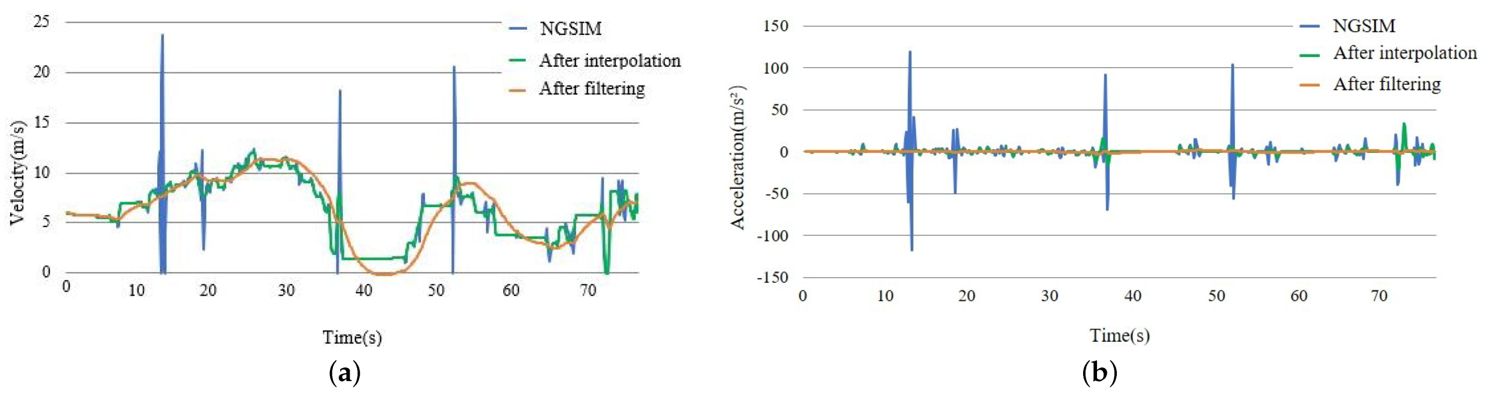
Used a Lagrange quintic polynomial (Equations (8) and (9)) to interpolate outliers’ coordinates.

$$\begin{array}{cc}\hfill l_k\left(x\right)& =\prod _{j=0,j\ne i}^n\frac{x-x_j}{x_k-x_j},\hfill \end{array}$$

(8)

$$\begin{array}{cc}\hfill L_n\left(x\right)& =\sum _{k=0}^n{l}_k\left(x\right)f\left(k\right),\hfill \end{array}$$

(9)

where $x_j,x_k$ are the interpolation joints, $f\left(x\right)$ is the interpolated function, $l_k\left(x\right)$ is a polynomial of degree n, and $L_n\left(x\right)$ is the Lagrange polynomial interpolation result.

(iii)

Used Kalman filter to eliminate the errors caused by observation and interpolation. Figure 3 shows the processed data changes. After the preprocessing, these data are more stable and practical.

4.2. Parameter Settings

(1)

Evaluation metrics

We evaluate the results in terms of the root mean square error (RMSE) of the predicted trajectories with respect to the actual future trajectories over a prediction horizon of 5 s. A smaller RMSE value indicates higher prediction accuracy of the model. Specifically, the prediction error at the future time-step t is as follows:

$$RMS{E}_t=\sqrt{\frac{{\sum }_{p=1}^m{\left(\widehat{x_p^t}-x_p^t\right)}^2+{\left(\widehat{y_p^t}-y_p^t\right)}^2}{m}},$$

(10)

where m is the number of test samples, and $\left(\widehat{x_p^t}-\widehat{y_p^t}\right)$ and $\left(x_p^t-y_p^t\right)$ denote the predicted and actual coordinates of vehicle p at time-step t, respectively.

(2)

Main parameters

The models involved in our experiment are all set up with the same hyperparameters for ensuring reliability. The encoder and decoder both have a 128-dimensional state, while the sizes of the convolutional layer and constraint representation are both 32. we adopt $Leaky\underline{}ReLU$ activation with $\alpha =0.1$ for all layers. In training, all models use an Adam optimizer with $\eta =0.001,{\beta }_1=0.9,$ and ${\beta }_2=0.999$. The $epoch$ and $batch\underline{}size$ are set as 128 and 8, respectively.

4.3. Compared Models

We compare the following models and system settings:

• Vanilla LSTM (V-LSTM): The V-LSTM is built on the seq2seq structure with an LSTM encoder and an LSTM decoder. As a basic model, it only takes the historical trajectory of target vehicle as input without considering other factors.
• LSTM with fully connected social pooling (S-LSTM): We implement this baseline according to [5]. Different from V-LSTM, the S-LSTM also incorporates historical trajectories of surrounding vehicles. The encoded representation of target vehicle and surrounding vehicles are fused with a fully connected layer before being sent to the decoder.
• LSTM with convolutional social pooling (CS-LSTM): Similar to S-LSTM, the CS-LSTM also incorporates historical trajectories of the target vehicle and surrounding vehicles. However, the CS-LSTM utilizes convolutional neural network to learn the interaction between target vehicle and surrounding vehicles. More details about CS-LSTM can be found in [4].
• Dynamic Context-aware Attention Network (DCAN): DCAN is implemented with an LSTM encoder and an attentional decoder described in Section 3, which are the same as our proposed DSCAN. It adds the attention mechanism to assign different weights to surrounding vehicles. We set this baseline model to demonstrate the effectiveness of constraint net.
• DSCAN: This is the complete model described in this paper, which is composed of the LSTM encoder, constraint net, and attentional decoder. Different from DCAN, DSCAN considers not only historical trajectories of the target vehicle and surrounding vehicles but also environment information.

4.4. Results

Table 1. Results: root mean squared prediction error (RMSE) values over a 5 s prediction horizon for the models compared.

Model	RMSE (m)
	1 s	2 s	3 s	4 s	5 s
V-LSTM	0.672	1.702	3.039	4.603	6.310
S-LSTM	0.628	1.365	2.226	3.249	4.516
CS-LSTM	0.63	1.366	2.211	3.244	4.489
DCAN	0.582	1.266	2.041	3.001	4.175
DSCAN	0.579	1.259	2.034	2.982	4.134

shows the RMSE values for the models being compared. Over the prediction horizon of 5 s, DSCAN outperforms the other models in terms of RMSE values, showing the effectiveness of our proposed model.

We note that the V-LSTM model produces higher RMSE values than other models at each time step. This model simply uses ego vehicle’s track history, while S-LSTM and CS-LSTM use information about the surrounding vehicles’ motion. This suggests that inter-vehicle interactions have a significant impact on trajectory prediction.

We also note that the RMSE value of the DCAN model is significantly reduced compared with that of the S-LSTM and CS-LSTM at each time step. In long-time prediction (5 s), DCAN improves the prediction accuracy by 7% compared to CS-LSTM. This shows that it is helpful to pay attention to the change of interaction over time. The attention mechanism provides different intermediate vectors during the prediction period instead of the same ones in CS-LSTM, which reduces information loss and is conducive to improving the trajectory prediction accuracy.

Finally, DSCAN, which uses both dynamic and static context information, further reduces the RMSE value. In particular, the prediction accuracy of DSCAN improves by 1% on top of that of DCAN at 5 s. This suggests that the static context information introduced through the constraint net also is a valuable cue for trajectory prediction. Vehicles on the highway can change the lane in the same direction but cannot cross the road boundary. Thus, the predicted trajectory should be constrained by lane boundaries, especially when the vehicle drives on both sides of the lanes. The constraint net makes the prediction tend toward the inside of the road rather than crossing the boundary to help DSCAN’s result be closer to the actual vehicle trajectory.

5. Discussion

One of the advantages of the attention mechanism is that the generated weights are interpretable. In this section, we analyze the prediction results made by our model to further understand its behavior.

5.1. Attention Distribution Analysis

The weights calculated at each time-step can be regarded as the normalization of the inter-vehicle interaction correlation. Over any predicted horizon t (t ≤ 5 s), the greater the weight of a grid, the more significant the vehicle’s impact on the research object’s motion. We visualize the attention weight in the reasoning process to further analyze the mechanism of our model (Figure 4). The findings are as follows:

(1) Weight value decays with distance: Overall, the weight of surrounding vehicles decreases as the distance to the research vehicle increases (Figure 4a). This feature is more prominent in the rear of the vehicle, but the local weight distribution in the front does not conform to it. It might be explained that, when driving forward, a safe distance is reserved ahead, and some farther vehicles in the front range have a greater impact on the research object. Beyond this range, the weight distribution fits the rule again. We also note that the neighborhood weights of the research object are negligible. This low probability distribution is also caused by safe driving distance.

(2) Weight distribution is directional: The most prominent finding that emerges from the analysis is that the front grids’ weight is greater than the rear grids’ weight. This is consistent with real scenarios. Drivers usually focus on the front to adjust themselves according to the motion of the front vehicles.

(3) The same-lane weight value is greater: Another finding is that the same lane’s grid weight is always greater than the adjacent lanes’ weight at the same distance. A possible explanation for this might be that a vehicle usually drives straight instead of changing lanes frequently. Since we average the values here, some great-weight instances of adjacent lanes are not displayed.

(4) The surrounding weight value tends toward an average as time increases: Over the predicted horizon, the most critical finding is that the weight values of great-weight grids decrease with time while small-weight grids are the opposite (Figure 4b). This result may be explained by the fact that the surrounding vehicles’ motion is uncertain in the future, and this uncertainty is accumulated over time. To reduce the cumulative impact of this uncertainty in long-term prediction, the attentional decoder pays attention to a larger vision. This leads to relatively decreased weight in a small range and relatively increased weight in a large range.

5.2. Scenario Analysis

Figure 5 shows the attention weight distribution with the predicted time under different scenarios, including left and right lane changes and driving straight. It is apparent that the attention weight is mainly distributed in the grids with vehicles. In the prediction process, DSCAN adaptively adjusts the distribution according to the vehicle motion. We note that the attention mechanism constantly adjusts to assign greater weight to the target lane as the lateral position changes. In particular, when changing to the right lane (scenario 2), the weight of the vehicle in the right front keeps getting larger. This inconsistency is due to the attentional decoder, which believes that the farther vehicle should be noticed after a few seconds. Our model with the attention is interaction-aware and can generate the corresponding different intermediate vectors, reducing information loss in the prediction process.

6. Conclusions

Considering the dynamic and static informaton encountered by vehicles in motion, this paper proposes a dynamic and static context-aware attention network (DSCAN) for trajectory prediction. We introduce the attention mechanism to adjust the weight distribution of inter-vehicle interaction during the prediction period. Moreover, we propose an extensible constraint net to extract multiple road structures. DSCAN is a multi-information fusion network in which the predicted results are close to real driving scenarios. Through the experiments on the real-world dataset, we demonstrate that DSCAN outperforms some existing LSTM-based trajectory prediction methods. Our proposed model provides insights for vehicle trajectory prediction and might be applied in autonomous driving system.

The generalizability of our results is subject to certain limitations. For instance, the dataset consists of only highway sections while the structure and traffic participants of common roads are more complex than ours. Further work needs to be conducted to incorporate these cues into the model. We believe that the DSCAN model will perform better with more information.

References

- Liu, Y.; Wang, X. Differences in Driving Intention Transitions Caused by Driver’s Emotion Evolutions. Int. J. Environ. Res. Public Health 2020, 17, 6962. [Google Scholar] [CrossRef]
- Park, S.H.; Kim, B.; Kang, C.M.; Chung, C.C.; Choi, J.W. Sequence-to-sequence prediction of vehicle trajectory via LSTM encoder-decoder architecture. In Proceedings of the 2018 IEEE Intelligent Vehicles Symposium (IV), Changshu, China, 26–30 June 2018; pp. 1672–1678. [Google Scholar]
- Sakata, N.; Kinoshita, Y.; Kato, Y. Predicting a pedestrian trajectory using seq2seq for mobile robot navigation. In Proceedings of the IECON 2018-44th Annual Conference of the IEEE Industrial Electronics Society, Washington, DC, USA, 21–23 October 2018; pp. 4300–4305. [Google Scholar]
- Deo, N.; Trivedi, M.M. Convolutional social pooling for vehicle trajectory prediction. In Proceedings of the IEEE Conference on Computer Vision and Pattern Recognition Workshops, Salt Lake City, UT, USA, 18–22 June 2018; pp. 1468–1476. [Google Scholar]
- Alahi, A.; Goel, K.; Ramanathan, V.; Robicquet, A.; Fei-Fei, L.; Savarese, S. Social lstm: Human trajectory prediction in crowded spaces. In Proceedings of the IEEE Conference on Computer Vision and Pattern Recognition, Las Vegas, NV, USA, 26 June–1 July 2016; pp. 961–971. [Google Scholar]
- Lefèvre, S.; Vasquez, D.; Laugier, C. A survey on motion prediction and risk assessment for intelligent vehicles. Robomech J. 2014, 1, 1–14. [Google Scholar] [CrossRef] [Green Version]
- Hillenbrand, J.; Spieker, A.M.; Kroschel, K. A multilevel collision mitigation approach—Its situation assessment, decision making, and performance tradeoffs. IEEE Trans. Intell. Transp. Syst. 2006, 7, 528–540. [Google Scholar] [CrossRef]
- Polychronopoulos, A.; Tsogas, M.; Amditis, A.J.; Andreone, L. Sensor fusion for predicting vehicles’ path for collision avoidance systems. IEEE Trans. Intell. Transp. Syst. 2007, 8, 549–562. [Google Scholar] [CrossRef]
- Batz, T.; Watson, K.; Beyerer, J. Recognition of dangerous situations within a cooperative group of vehicles. In Proceedings of the 2009 IEEE Intelligent Vehicles Symposium, Xi’an, China, 3–5 June 2009; pp. 907–912. [Google Scholar]
- Ammoun, S.; Nashashibi, F. Real time trajectory prediction for collision risk estimation between vehicles. In Proceedings of the 2009 IEEE 5th International Conference on Intelligent Computer Communication and Processing, Cluj-Napoca, Romania, 27–29 August 2009; pp. 417–422. [Google Scholar]
- Althoff, M.; Mergel, A. Comparison of Markov chain abstraction and Monte Carlo simulation for the safety assessment of autonomous cars. IEEE Trans. Intell. Transp. Syst. 2011, 12, 1237–1247. [Google Scholar] [CrossRef] [Green Version]
- Atev, S.; Miller, G.; Papanikolopoulos, N.P. Clustering of vehicle trajectories. IEEE Trans. Intell. Transp. Syst. 2010, 11, 647–657. [Google Scholar] [CrossRef]
- Kumar, P.; Perrollaz, M.; Lefevre, S.; Laugier, C. Learning-based approach for online lane change intention prediction. In Proceedings of the 2013 IEEE Intelligent Vehicles Symposium (IV), Gold Coast, QLD, Australia, 23–26 June 2013; pp. 797–802. [Google Scholar]
- Qiao, S.; Shen, D.; Wang, X.; Han, N.; Zhu, W. A self-adaptive parameter selection trajectory prediction approach via hidden Markov models. IEEE Trans. Intell. Transp. Syst. 2014, 16, 284–296. [Google Scholar] [CrossRef]
- Houenou, A.; Bonnifait, P.; Cherfaoui, V.; Yao, W. Vehicle trajectory prediction based on motion model and maneuver recognition. In Proceedings of the 2013 IEEE/RSJ International Conference on Intelligent Robots and Systems, Tokyo, Japan, 3–7 November 2013; pp. 4363–4369. [Google Scholar]
- Schlechtriemen, J.; Wirthmueller, F.; Wedel, A.; Breuel, G.; Kuhnert, K.D. When will it change the lane? A probabilistic regression approach for rarely occurring events. In Proceedings of the 2015 IEEE Intelligent Vehicles Symposium (IV), Seoul, Korea, 28 June–1 July 2015; pp. 1373–1379. [Google Scholar]
- Leon, F.; Gavrilescu, M. A Review of Tracking and Trajectory Prediction Methods for Autonomous Driving. Mathematics 2021, 9, 660. [Google Scholar] [CrossRef]
- Xu, K.; Qin, Z.; Wang, G.; Huang, K.; Ye, S.; Zhang, H. Collision-free lstm for human trajectory prediction. In International Conference on Multimedia Modeling; Springer: Cham, Switzerland, 2018; pp. 106–116. [Google Scholar]
- Gupta, A.; Johnson, J.; Fei-Fei, L.; Savarese, S.; Alahi, A. Social gan: Socially acceptable trajectories with generative adversarial networks. In Proceedings of the IEEE Conference on Computer Vision and Pattern Recognition, Salt Lake City, UT, USA, 18–22 June 2018; pp. 2255–2264. [Google Scholar]
- Xu, Y.; Zhao, T.; Baker, C.; Zhao, Y.; Wu, Y.N. Learning trajectory prediction with continuous inverse optimal control via Langevin sampling of energy-based models. arXiv 2019, arXiv:1904.05453. [Google Scholar]
- Yoon, Y.; Kim, T.; Lee, H.; Park, J. Road-aware trajectory prediction for autonomous driving on highways. Sensors 2020, 20, 4703. [Google Scholar] [CrossRef]
- Staudemeyer, R.C.; Morris, E.R. Understanding LSTM—A tutorial into Long Short-Term Memory Recurrent Neural Networks. arXiv 2019, arXiv:1909.09586. [Google Scholar]
- Choi, D.; Yim, J.; Baek, M.; Lee, S. Machine Learning-Based Vehicle Trajectory Prediction Using V2V Communications and On-Board Sensors. Electronics 2021, 10, 420. [Google Scholar] [CrossRef]
- Lee, N.; Choi, W.; Vernaza, P.; Choy, C.B.; Torr, P.H.; Chandraker, M. Desire: Distant future prediction in dynamic scenes with interacting agents. In Proceedings of the IEEE Conference on Computer Vision and Pattern Recognition, Honolulu, HI, USA, 21–26 July 2017; pp. 336–345. [Google Scholar]
- Das, S.; Dutta, A.; Sun, X. Patterns of rainy weather crashes: Applying rules mining. J. Transp. Saf. Secur. 2020, 12, 1083–1105. [Google Scholar] [CrossRef]
- Zhu, D.; Shen, G.; Liu, D.; Chen, J.; Zhang, Y. FCG-aspredictor: An approach for the prediction of average speed of road segments with floating car GPS data. Sensors 2019, 19, 4967. [Google Scholar] [CrossRef] [Green Version]
- Dey, K.C.; Rayamajhi, A.; Chowdhury, M.; Bhavsar, P.; Martin, J. Vehicle-to-vehicle (V2V) and vehicle-to-infrastructure (V2I) communication in a heterogeneous wireless network–Performance evaluation. Transp. Res. Part C 2016, 68, 168–184. [Google Scholar] [CrossRef] [Green Version]
- Milanés, V.; Villagrá, J.; Godoy, J.; Simó, J.; Pérez, J.; Onieva, E. An intelligent V2I-based traffic management system. IEEE Trans. Intell. Transp. Syst. 2012, 13, 49–58. [Google Scholar] [CrossRef] [Green Version]
- Cheng, H.T.; Koc, L.; Harmsen, J.; Shaked, T.; Chandra, T.; Aradhye, H.; Shah, H. Wide & deep learning for recommender systems. In Proceedings of the 1st Workshop on Deep Learning for Recommender Systems, Boston, MA, USA, 15 September 2016; pp. 7–10. [Google Scholar]
- Guo, H.; Tang, R.; Ye, Y.; Li, Z.; He, X. DeepFM: A factorization-machine based neural network for CTR prediction. arXiv 2017, arXiv:1703.04247. [Google Scholar]
- Bahdanau, D.; Cho, K.; Bengio, Y. Neural machine translation by jointly learning to align and translate. arXiv 2014, arXiv:1409.0473. [Google Scholar]
- Xu, K.; Ba, J.; Kiros, R.; Cho, K.; Courville, A.; Salakhudinov, R.; Zemel, R.; Bengio, Y. Show, attend and tell: Neural image caption generation with visual attention. In Proceedings of the 32nd International Conference on Machine Learning, Lille, France, 6–11 July 2015; pp. 2048–2057. [Google Scholar]
- Chorowski, J.; Bahdanau, D.; Serdyuk, D.; Cho, K.; Bengio, Y. Attention-based models for speech recognition. arXiv 2015, arXiv:1506.07503. [Google Scholar]
- Rush, A.M.; Chopra, S.; Weston, J. A neural attention model for abstractive sentence summarization. arXiv 2015, arXiv:1509.00685. [Google Scholar]
- Lin, L.; Gong, S.; Peeta, S.; Wu, X. Long Short-Term Memory-Based Human-Driven Vehicle Longitudinal Trajectory Prediction in a Connected and Autonomous Vehicle Environment. Transp. Res. Rec. 2021. [Google Scholar] [CrossRef]
- Montanino, M.; Punzo, V. Making NGSIM data usable for studies on traffic flow theory: Multistep method for vehicle trajectory reconstruction. Transp. Res. Rec. 2013, 2390, 99–111. [Google Scholar] [CrossRef]