Comparison of Ecohydrological and Climatological Zoning of the Cities: Case Study of the City of Pilsen

Abstract

Standardized delimiting of local climate zones (LCZ) will be better applicable to the urban adaptation to climate change when the ecohydrological properties of LCZ units are known. Therefore, the properties of LCZ units based on the methodology of ecohydrological zoning of the urban landscape, which was created in GIS as a basis for planning blue-green infrastructure of cities in the Czech Republic, are presented in the paper. The goal of this study is to compare approaches and results of our own ecohydrological zonation and standardized LCZ delimiting in the city of Pilsen. Both methodological approaches differ in input data, resolution details and parameters used. The results showed that the areas of the individual LCZ classes show different levels of ecohydrological qualities. Internal heterogeneity of LCZ classes demonstrated by variance of ecohydrological parameters’ values can be partly explained by different techniques and data sources for delimitation of both zonations, but by different sets of delimitation criteria. The discussion is held on the importance of terrain slope for supplementing the LCZ classification. A case study can be a stimulus for further development of holistic urban zoning methodologies that would take into account both climatological and ecohydrological conditions.

1. Introduction

All cities are considered to be vulnerable systems due to ongoing climate changes [1,2]. Depending on the macroclimate position, as well as land cover structure of the urbanized landscape, quite obvious consequence of climate change has been the occurrence of urban heat islands (UHI) and surface urban heat islands (SUHI) [3,4]. Depending on the urban forms of built-up areas and the characteristics of green infrastructure at the level of micro-scale, UHI has a negative impact on the thermal comfort of citizens [5]. Climate change, however, causes an extreme level of hydrologic regime in an urban landscape [6,7]. On one hand, municipalities have to solve problems related to droughts, lack of groundwater and a limited amount of natural moisture for urban greenery [8,9,10]. On the other hand, they have to introduce measures to mitigate the impacts of heavy rains, floods on a built-up area of a city, capacity overload of drainage systems that cause negative impact on quality of water in watercourses [2,8]. The abovementioned issues became relevant for the cities in Central Europe as well [4,11,12].

The planning for adaptation of cities to climate changes must interlink a traditional approach of urban and strategic planning with modern scientific knowledge of urban climatology and urban hydrology, which contribute to the design of effective measures for specific types of sites in the city [7,13]. Methodological procedures are being developed that integrate adaptation measures into complex environmental tools for practice [14]. An important part of the interconnection of hydrological and climatological models is the balance of energy flows [15]. The concept of blue-green infrastructure (BGI) is often recommended as a suitable tool for city adaptation [16,17,18]. Using BGI is presented as a new system for stormwater management, which supports the quality and the retention of water in the urban landscape. Moreover, it is beneficial for public space, for adaptation to climate change, as well as for biodiversity [18]. Unlike traditional approaches that are focused on technical solution to drain stormwater through combined sewerage as quick as possible out of the urban areas, BGI is designed as a system similar to natural water circulation. It connects green infrastructure as an organized system of urban greenery and stormwater management in the city [17]. It can always be problematic, when two approaches—a technical one and a nature-based one—are differentiated in a simplifying way [19]. Thus, there are blended terminologies occurring in the literature, such as blue-green-gray [20], hybrid or mixed infrastructure [21].

The urban planning of sustainable cities requires specialized maps that visualize spatial differentiation of the urban landscape according to appropriate environmental parameters [14]. Based on the definition of local climate zones (LCZ), tools for modeling of urban climate have been developed that can be used for the purpose of planning for adaptation measures [22,23,24]. Professional discussion on the LCZ delimitation has been happening in terms of scale of spatial units processed via GIS-based [25,26,27], selection of thermal analysis techniques [28,29] or automatic data processing [27,29]. The current analysis of European LCZ studies shows the need to focus on the refining LCZ and higher accuracy in defining training areas [28].

Different properties of LCZ affect thermal comfort mainly through evaporation depending on air flow and the effect of green infrastructure [30,31]. Thermal comfort conditions have a significant daily regime [32]. What is good about LCZ when the urban climate is modeled, is that they can be also used for making scenarios on how the development of the urbanized landscape impact climatic conditions or for assessment of proposed adaptation measure’s impact. LCZ application is usually focused on urban climate modelling, on UHI intensity delimitation, on thermal comfort assessment [28] eventually on energy balance of buildings, especially in terms of building carbon emission [33]. Standardized LCZ units can also be used as a basis for assessing the impact of urban landscape transformation on ecosystem services [34]. An important factor, which influences UHI intensity, is how the BGI elements are spatially distributed in the city [11,35]. Thus, it is expected that there are certain causalities across LCZ classes and spatial characteristics of BGI in cities. Discovering these causalities would enable the application of a world-wide standardized process of LCZ definition to broader scale of climate change impacts in cities. This intention is consistent with a trend to strengthen multidisciplinary approaches of adaptation measures that should not only help to decrease thermal discomfort of citizens [11,14] but also contribute to the solution of extreme hydrological events [19], to support biodiversity in cities [36] and enhance the quality of public space [37]. Holistic approaches become the basis for integrated planning methodology for sustainable development of cities [38].

This study is focused on the links between LCZ and ecohydrological qualities in our paper. Only a few studies dealing with interactive models between energy and water in urban areas have been focused on the linkages between LCZ and hydrologic processes [15,39,40]. A dominant link of this interaction is a process of evapotranspiration [40,41,42]. Our research is focused especially on a relationship between LCZ and the runoff regime of areas in a context with BGI elements.

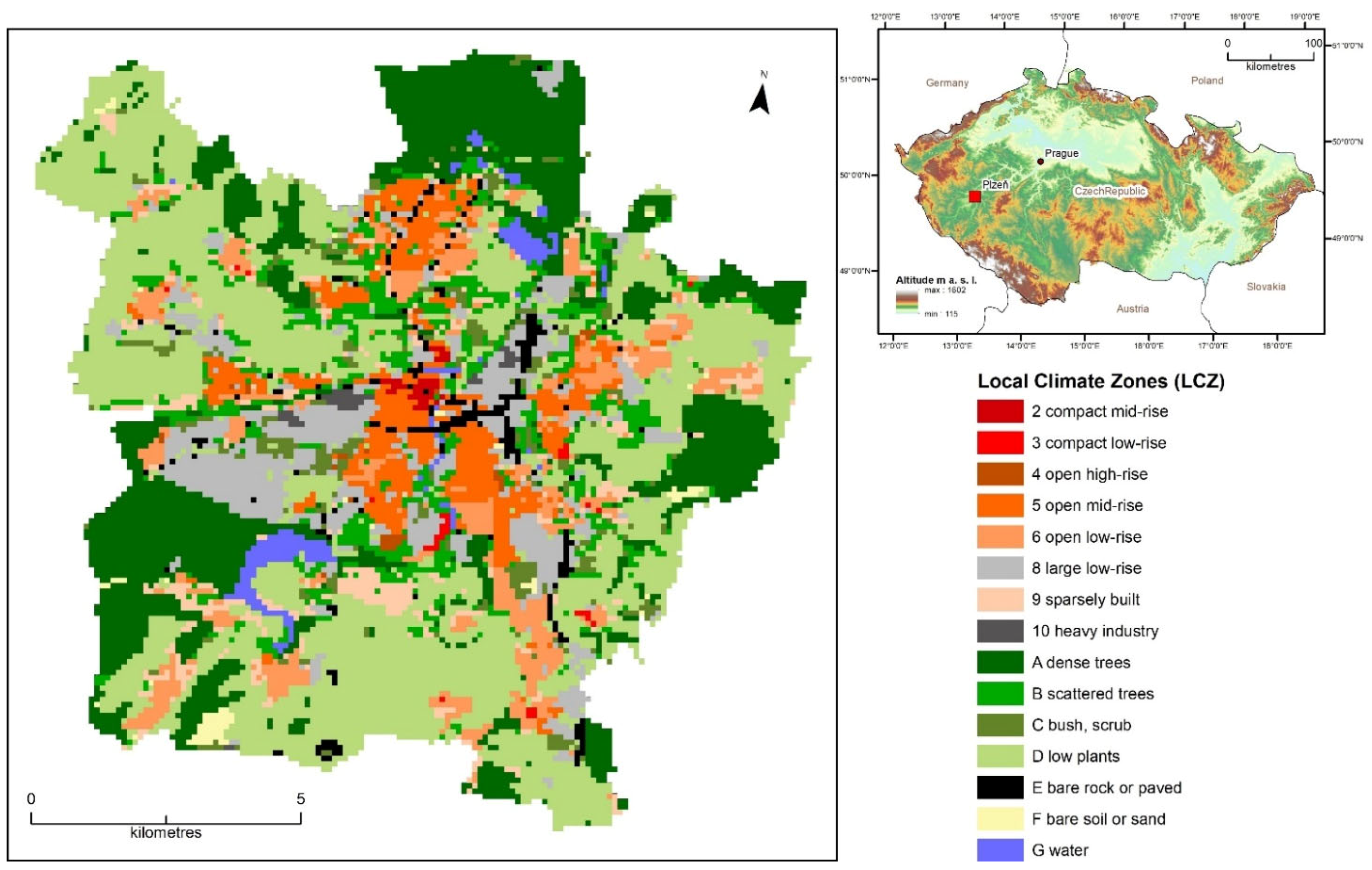
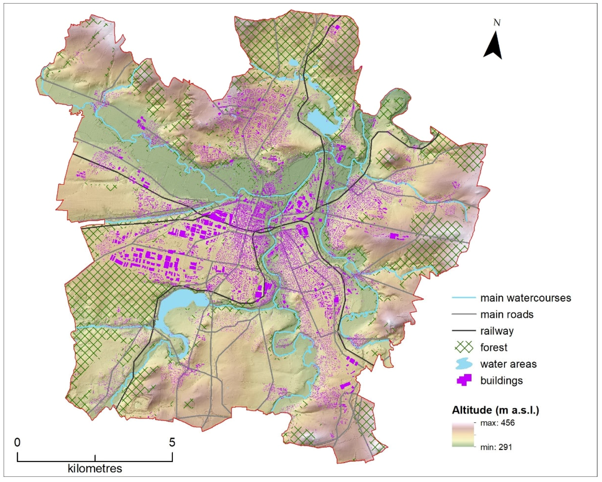
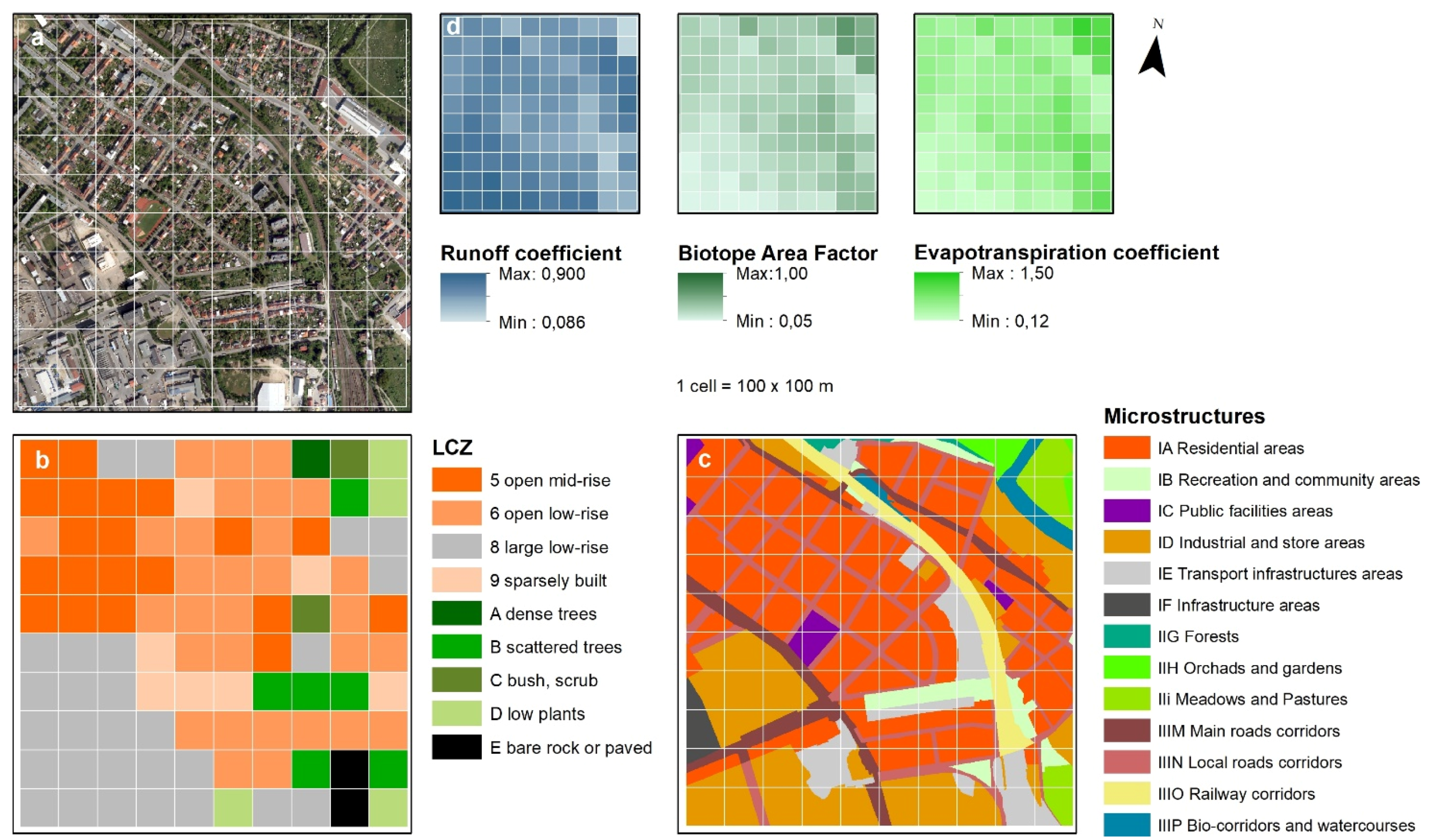
The analysis of geodata is based on a case study of the city of Pilsen (Czech Republic), for which previous projects defined and demarcated LCZ [43], as well as ecohydrological spatial units with a link to BGI proposals. Both zonations in the city come up from different geodata and their spatial units have different scales. This fact reflects in a methodology of the analysis. That is why the authors first present the methodology of ecohydrological zonation in an urban landscape, which was made in GIS as a basis for blue-green infrastructure planning in Czech cities.

The goal of the analysis is to compare the ecohydrological zonation of the territory of the city with the standardized climatological zonation based on LCZ. A fundamental question of our study is whether defining of LCZ can help to plan measures not only to mitigate thermal stress, plus also provide more complexed adaptation measures that take into account other climate changes impacts, especially extreme hydrological events.

2. Materials and Methods

2.1. Study Area

The city of Pilsen (population 170.5 thousand inhabitants), the dominant core of the settlement system in the western part of the Czech Republic, was chosen as a model city for the comparison of ecohydrological and climatological zoning. The natural conditions of the territory of the city are influenced by its location at the confluence of four rivers (Figure 1). The altitude of Pilsen varies between 293–452 m above sea level [44]. The city center is surrounded by individual city districts, all situated on flat terrain ridges and river terraces. The individual built-up parts of the city are separated from each other by river valleys, often accompanied by green areas. There are two large industrial areas and a radially arranged network of road and railway corridors, all leading outside of floodplains, belong to specific elements of compact built-up areas of the city of Pilsen. There are individual satellite settlements in the suburban landscape, which consists mainly of agricultural land and forest units.

According to land use statistics based on the real estate records in the cadastral area of Pilsen (137.7 km²), 43% of the total area is agricultural land (31% arable land, 7% gardens and 5% meadows and pastures). Water areas make up cumulatively 3% of the total area of the city. Urbanized parts of the city cadaster are mainly in the category of built-up areas and courtyards (7%) and other areas (28%), respectively [45]. The category “other areas“ includes a number of other land use options, often for public benefit functions, such as traffic routes, sports and recreational areas, urban green areas, cemeteries, landfills or unusable areas.

Average air temperature measured at the Pilsen-Mikulka station in the period 2006–2015 was 9.5 °C [45]. While in the period between 1971–2000 the average January temperature was –1.6 °C and that of July was 18 °C, between 2006–2015 the average January temperature was –0.1 °C and that of July was 20 °C [44]. The average annual rainfall in 2006–2015 recorded at the Pilsen-Mikulka station was 514.8 mm [45]. According to the standardized values of the Czech Hydrometeorological Institute for the period 2005–2015 for the station Pilsen-Mikulka, a thirty-minute rain with a periodicity of repetition n = 1 year causes a direct specific runoff of 115.6 liters per second per hectare [19].

2.2. Methodology of Ecohydrological Zoning of the City

2.2.1. Choice of Two-Level Categorization of the Territory

The actual approach of ecohydrological evaluation of the urban landscape has been inspired by the methodology of evaluation of the cities of Munich and Rotterdam [46,47], but adjusted to the needs of ecohydrological zoning and available geodata. Due to the nature of official statistics, common records of the type and the way the yards are individually used, it is not possible to simply use either the databases of the real estate cadaster or master plan for determination of concrete characteristics of surfaces. An ideal source of data in terms of territorial accuracy and parameterization can be multispectral aerial photography with accurate resolution [48]. This method, however, is not standardly available in the Czech Republic. Our methodology of ecohydrological evaluation is based on a two-level categorization of territorial units of the urban landscape (Figure 2). The levels are in compliance with topical and choric dimensions of urban landscape [49]. For database processing and map generating, following items have been distinguished (a) elementary surfaces—territorial units of topical dimension that have quasi-homogeneous ecohydrological characteristics (e.g., lawn, water area, a roof of the building) and (b) microstructures in urban landscape—territorial units of choric dimension. Microstructures are composed of a combination of elementary surfaces of a certain typical composition and a certain use, which have collectively and functionally common features, e.g., loose development of family houses or heavy industry areas.

The categorization of territorial units is based on the possibility of determining some parameters of ecohydrological features for types of elementary areas (e.g., infiltration, evapotranspiration, runoff) and some parameters for functional spatial units (e.g., typical level of runoff water pollution). Parameters at the microstructure level can be based on standardization of values and thus express benchmarks for development regulations, e.g., determination of urban greening indicator for newly emerging parts of the development. At the level of microstructures of the urban landscape, we can organize water management in a decentralized unit [8]. Recommended measures of blue-green infrastructure are also often linked to the typology of similar urban units in studies and methodologies [9,46,50]. The methodology of ecohydrological evaluation of the area was verified during the creation and processing of ecohydrological maps of Pilsen and Ústí nad Labem in 2017 [45].

2.2.2. Definition and Classification of the Microstructures

The definition of microstructures and their classification into types and subtypes was performed using a cadastral map, master plan, orthophoto, registry of territorial identification, addresses and real estates (RÚIAN), technical maps of the city and digital base of water management data (DIBAVOD) (

Table 1. Datasets used for delimiting and analysis of microstructures and elementary areas.

Dataset	Year	Attribute	Source	Use
Basic functional areas	2011	polygons of function areas by master plan	Municipality of the city of Pilsen	Delimiting of microstructures and identification of types
Technical map	2017	polygons of roads and streets
Cadaster of real estate	2016	state administration systems of descriptive and geodetic information	Czech Office for Surveying, Mapping and Cadaster
RÚIAN	2016	registry of territorial identification, addresses and real estates
DIBAVOD	2010	digital base of water management data—polygons of water bodies	T. G. Masaryk Water Research Institute	Identification of water bodies
3D model of the city	2017	building multipatch layer	Municipality of the city of Pilsen	Refinement and replenishment of the ground plan of buildings
Orthophoto	2014	orthophoto in vegetation period, raster resolution 0.25 m	Czech Office for Surveying, Mapping and Cadaster	Delimiting and classification of the elementary areas
Green space inventory	2017	polygons of public green space inventory	Municipality of the city of Pilsen	Delimiting and classification of greenery and calibration of autoclassification results
DMR 5G	2013	digital terrain model of the Czech Republic of the 5th generation (DMR 5G)	Czech Office for Surveying, Mapping and Cadaster	Addition of greenery classification, slope analysis
DMP 1G	2013	digital surface model of the Czech Republic of the 1st generation (DMP 1G)

).

Each microstructure was defined as a cluster of cadastral map areas, corresponding to a certain category. The definition of microstructures from spatial data took place in the first step by assigning attribute information on the method and type of land use to areas (

Table 2. Categorization of microstructures.

Classes of Microstructures	Types of Microstructures		Subtypes of Microstructures
I Urban areas	IA	Residential areas	IA1	Compact urban built-up areas
			IA2	Urban built-up areas
			IA3	Low density urban built-up areas
			IA4	Detached house areas
			IA5	Low density detached house areas
			IA6	Rural built-up areas
	IB	Recreation and community areas	IB1	Public green areas
			IB2	Public impervious areas
			IB3	Private recreation areas
			IB4	Gardening community areas
	IC	Public facilities areas	IC1	Large shops and services areas
			IC2	Small and medium shops and services areas
			IC3	School and sports facilities
	ID	Industrial and store areas	ID1	Heavy industry areas
			ID2	Light industry and store areas
	IE	Transport infrastructure areas	IE1	Road infrastructure areas
			IE2	Railways’ infrastructure areas
	IF	Infrastructure areas	IF1	Technical infrastructure areas
			IF2	Water infrastructure areas
			IF3	Waste management areas
II Peri-urban areas	IIG	Forests
	IIH	Orchards and gardens
	III	Meadows and pastures
	IIJ	Arable land
	IIK	Water areas	IIK1	Ponds
			IIK2	Water reservoirs
	IIL	Wetlands
III Corridors	IIIM	Main road corridors	IIIM1	Main urban roads
			IIIM2	Main extra-urban roads and highways
	IIIN	Local road corridors	IIIN1	Local transit streets
			IIIN2	Local living streets
			IIIN3	Local extra-urban road
	IIIO	Railways
	IIIP	Bio-corridors and watercourses	IIIP1	River corridors
			IIIP2	Brook corridors
			IIIP3	Green and episodic runoff corridors

, Figure 2). Next, layers of areas with the same type of use were created and subsequently neighboring areas were dissolved in order to create a continuous layer with identical use. Then, the layers were joined according to the functional use. This procedure was not applied at once for the whole territory of Pilsen. Rather, the territory was divided into sections and in them the procedure was gradually implemented. The last step was to merge the sections. The result was gradually checked from the topology point of view, and the space delimitation logic with possible error correction was verified. 7,494 microstructures of various types were defined in the entire administrative territory of the city of Pilsen [45]. The areas of the individual units vary greatly depending on the types of microstructures. The area of microstructures in the whole set (average = 20,624 m², median = 2395 m², n = 7494) ranges from the smallest street segments (minimum = 114 m², IE1—road infrastructure areas) to large blocks of forest cover (maximum = 4,765,340 m², IIG—forests). In category IA (residential areas, n = 1617), the average area of microstructures is 10,254 m² and the median area is 7486 m².

The choice of categories of microstructures partially respects the functional categories of the zoning plan (Table 2). The main types of categories are divided into three basic classes: (I) urban areas—polygonal microstructures predominantly with buildings and artificial surfaces, (II) peri-urban areas—polygonal microstructures predominantly without buildings, (III) corridors—linear microstructure. Linear microstructures are divided into sub-sections as individual territorial units. At the same time, they form the boundaries of polygonal microstructures. Linear microstructures were, unlike the other methodologies [46,47], defined as separate territorial units, because they are essential for blue-green infrastructure planning as drain lines or connecting green belts in public space.

2.2.3. Classification of Elementary Areas

Identification and classification of elementary areas with a resolution of 0.5 m was performed on the basis of underlying geodata (Table 1): orthophoto, registry of territorial identification, addresses and real estates (RÚIAN), green space inventory, technical map, digital terrain model of the Czech Republic of the 5th generation (DMR 5G), digital surface model of the Czech Republic of the 1st generation (DMP 1G) and it was selectively verified by detailed mapping at several localities. The digital surface model of the Czech Republic of the 1st generation (DMP 1G) represents a picture of the territory including buildings and vegetation cover in the form of irregular network (TIN). The models DMP 1G and DMR 5G (georelief) are based on the data acquired by altimetry airborne laser scanning of the Czech Republic territory between the years 2009 and 2013 [45].

Orthophoto was categorized by unsupervised classification using the already tested ISOADATA algorithm into 10 categories. The classified raster (pixel resolution 0,5 m) was subjected to zonal statistics together with vector layers from the green space inventory, DIBAVOD and modified layers of buildings and roads. Based on the statistical results, the categorization of the raster was simplified to permeable surfaces (green spaces bare soil, water areas), impermeable surfaces and unspecified areas (shadows of buildings predominantly). The classification of elementary areas was further specified and supplemented on the basis of additional available detailed layers, such as the green passport, updated layers of buildings and layers of roads. The result was a grid with 9 categories of elementary surfaces (water, arable land, bare land, trees, bush, meadows and pastures, greenery, impermeable surfaces, buildings and other/unspecified). The category “greenery“ was further specified on the basis of a green spaces inventory and using a normatively entered height based on the analysis of digital surface and terrain models (

Table 3. Categorization of elementary areas.

Types of Elementary Areas	Subtypes
1 Roofs
2 Impervious surfaces
3 Semi-permeable surfaces
4 Bare land
5 Greenery	5a Lawns
	5b Shrubs
	5c Trees
	5d Flowerbeds
6 Water areas
7 Meadows and pastures
8 Arable land
9 Forests

). There was a manual correction of places with problematic identification.

2.2.4. Parameterization of Microstructures

The microstructures were further evaluated based on the parameters of the elementary surfaces. This was done by calculating the statistics of the raster areas in each microstructure. Elementary surface types, assigned in the catalogue, have values of coefficients related to their characteristics—runoff, infiltration, evapotranspiration, run-off water’s pollution risk and ecosystem services. Three parameters were selected for comparison with LCZ definition: runoff coefficient, evapotranspiration coefficient and biotope area factor (BAF) chosen as an index for the assessment of green infrastructure [51].

The runoff coefficient expresses the relative share of run-off water from precipitation, taking into account the type of surface and the inclination of the area [9]. More precisely, it is possible to define the runoff coefficient as the share of the runoff of the water of the standardized rain of the considered periodicity in the Czech state standard 75 6101. Tabular values of the coefficient (interval 0–1) prove the differences in the type of surface permeability and take into account the category of the inclination of the area. We determined the inclination based on the accurate digital terrain model (DMR 5G), which, however, does not identify the slope of roofs.

The basic process connecting the blue-green infrastructure and the hydrological cycle with a thermoregulatory effect on an urbanized area is transpiration. In this sense, evapotranspiration, together with retention due to vegetation, is a key process of blue-green infrastructure [11]. The evapotranspiration coefficient used expresses the relative relationship to the so-called reference evapotranspiration according to the FAO methodology, which is based on potential evapotranspiration of normalized turfgrass [52]. The evapotranspiration coefficient (in the range 0–1.5) was determined in tabular form on the basis of the calculation of the values “plant factor” and “leaf area index” (LAI) according to available methodologies [53,54], taking into account Czech climatic conditions. The actual evaporation from the areas depends not only on their nature, but also on the course of meteorological conditions during each day [55]. The availability of water for evaporation is significantly affected by previous precipitation or artificial watering of urban greenery.

Another parameter was the biotope area factor (BAF), which in various variants is generally used as a reference index for the assessment of green infrastructure in urban areas [51,56,57,58]. The use of BAF categorization has been adapted to the possibilities of area type identification. The BAF parameters (in the interval 0–1) were used as relative values that best describe the level of ecosystem services of green spaces [59].

2.3. Methodology of Comparison of Ecohydrological Zoning and Local Climatic Zones

Delimited local climate zones (LCZ) is the basic climatological zoning of cities introduced by [24] and subsequently modified by [60]. The classification of 17 basic classes is divided into two categories: built types and land cover types. The LCZ classes are defined according to physical characteristics of environment, such as building surface fraction—BSF, impervious surface fraction—ISF, pervious surface fraction—PSF, geometric average of building heights—HRE etc. In 2019, the LCZ were defined for Pilsen in the project for identification of locations vulnerable to thermal stress [43]. The classification method, which was used [61], works as one of the few directly with defined features of the environment, specifically with their values in cells measuring 100 × 100 m, which are the basic input parameters of the classification algorithm. Each cell is assigned to the LCZ class that best matches the typical physical properties of the environment. Subsequently, cell clusters are defined as the basic units of LCZ (Figure 3). A detailed introduction of the classification algorithm is published in the work [61]. The method used for the delineation of local climate zones presented here was developed and tested in the area of Brno and its surroundings. It was validated in the cities of Hradec Králové and Olomouc and their surroundings (Czech Republic) [30]. The definition of LCZ for the city of Pilsen was based on following sources: the GMES Copernicus databases, OpenStreet Maps, the Czech Office for Surveying, Mapping and Cadaster and urban territorial data [61].

The comparison of the actual definition of ecohydrological units, i.e., the microstructures of the urban landscape, and the definition of standardized LCZ was carried out in three steps on the territory of the city of Pilsen. First, a matrix was generated on the basis of statistics in GIS, which characterizes the distribution of the entire cadastral area of Pilsen according to the types of microstructures and LCZ classes. The relative representation of individual types of microstructures was calculated for individual LCZ classes. The analysis of the results focused on the built types of LCZ classes, which are essential for the creation of UHI. Due to significant differences in the frequency of occurrence of LCZ classes, we focused in more detail on the four that are most represented in Pilsen: LCZ 5, LCZ 6, LCZ 8 and LCZ 9.

In the next step, parameterization of LCZ raster cells measuring 100 × 100 m is performed (Figure 4). As basic ecohydrological parameters for the spatial analysis, the runoff coefficient, the evapotranspiration coefficient and the biotope area factor have been chosen. To assign a parameter to LCZ cells of a grid measuring 100 × 100 m, the average of the values of the parameters of microstructures represented in the centers of the grid measuring 5 × 5 m was used. Thus, the parameter of each LCZ raster cell is the average of 400 values.

In the third step, the built types of the LCZ class were compared in terms of the calculated ecohydrological parameters. Descriptive statistics of parameters assigned to 100 × 100 m raster cells in individual LCZ classes were compared. For the four most important classes, we focused in more detail on the assessment of variability and distribution of data sets. The results were assessed and explained with regard to the selected parameters. Subsequently, possible use of the standardized definition of LCZ for the evaluation of ecohydrological conditions of the urban area were discussed. Differences among the LCZ classes (LCZ 5–LCZ 9) results for runoff coefficient, evapotranspiration coefficient and biotope area factor were tested using Kruskall–Wallis test (the assumption of homogeneity via Levene test) with non-parametric post hoc comparison (Bonferroni correction of p value).

3. Results

3.1. The Structure of LCZ Classes according to Microstructure of Urban Landscape

The matrix of results shows the representation of individual types of microstructures in individual classes of LCZ (Appendix A,

Table A1. Relative representation of microstructure types in individual LCZ classes (%).

MS	Local Climate Zone Classes
	2	3	4	5	6	8	9	10	A	B	C	D	E	F	G
IA1	50.9	0.0	0.8	2.3	0.0	0.0	0.0	0.0	0.0	0.0	0.0	0.0	0.5	0.0	0.3
IA2	13.8	13.3	0.0	12.6	0.7	0.8	0.3	0.2	0.0	0.3	0.0	0.0	0.8	0.2	0.4
IA3	0.0	1.3	59.5	33.9	3.3	1.6	1.5	0.0	0.1	2.0	0.7	0.2	2.2	1.1	0.0
IA4	0.0	15.8	1.3	7.6	35.6	0.5	9.2	0.0	0.1	1.2	0.8	0.3	1.5	2.4	0.0
IA5	0.0	0.0	0.3	0.6	15.3	0.4	17.8	0.0	0.5	2.9	0.7	0.7	0.6	3.1	0.1
IA6	0.0	33.6	0.0	0.7	12.0	0.5	5.1	0.0	0.0	0.8	0.4	0.2	0.1	0.0	0.0
IB1	3.3	1.0	4.7	2.7	1.1	1.0	2.7	0.8	2.2	21.3	10.4	0.8	3.3	0.6	1.8
IB2	2.3	0.0	0.0	0.1	0.0	0.1	0.0	0.0	0.0	0.2	0.0	0.0	0.7	0.0	0.0
IB3	0.0	0.0	0.0	0.0	1.7	0.1	22.0	0.0	0.5	5.4	0.4	0.5	0.0	0.0	0.8
IB4	0.0	1.2	0.0	0.2	0.7	0.3	4.5	0.0	0.3	9.7	0.9	0.6	0.4	0.0	0.6
IC1	0.1	0.0	0.6	3.9	0.1	8.2	0.1	0.0	0.0	0.7	0.7	0.3	2.8	0.1	0.0
IC2	2.0	0.0	1.7	2.2	0.2	1.9	0.7	0.0	0.0	0.3	0.2	0.1	2.8	0.0	0.4
IC3	0.0	0.0	9.5	7.4	1.3	3.7	1.6	0.0	0.5	5.0	2.8	1.8	2.4	2.1	2.2
ID1	0.0	1.9	0.0	0.1	0.0	10.6	0.0	73.2	0.3	0.4	3.7	0.0	2.8	0.5	0.0
ID2	0.4	6.2	4.3	1.5	1.5	45.7	2.5	16.1	0.5	3.1	9.0	0.9	6.3	5.5	0.5
IE1	0.3	1.5	0.3	0.6	0.4	2.1	0.5	0.1	0.1	0.8	0.4	0.1	4.8	1.6	0.1
IE2	0.0	0.0	0.0	0.2	0.0	1.7	0.0	1.9	0.0	0.3	1.5	0.0	24.3	0.4	0.0
IF1	0.1	0.0	0.0	0.0	0.0	2.2	0.4	3.8	0.6	0.7	2.8	0.3	0.2	48.0	0.1
IF2	0.0	0.2	0.0	0.1	0.1	2.3	0.1	0.1	0.2	0.6	0.2	0.3	0.1	0.0	0.3
IF3	0.0	0.0	0.0	0.0	0.0	0.3	0.0	0.0	0.2	0.2	0.0	0.3	0.0	12.7	0.0
IIG	0.0	0.3	0.0	0.1	0.8	0.8	4.0	0.0	84.5	8.0	10.3	1.9	1.1	4.1	3.3
IIH	0.0	0.7	0.0	0.3	0.7	0.5	1.3	0.0	0.4	5.3	5.4	0.7	0.5	1.4	0.5
III	0.0	0.1	1.2	0.6	1.8	2.6	4.7	0.0	1.8	9.8	35.0	11.9	5.6	7.9	0.5
IIJ	0.0	0.1	0.0	0.1	1.4	1.7	6.4	0.0	2.0	5.0	4.2	71.8	2.1	4.0	0.4
IIK1	0.0	0.0	0.0	0.0	0.1	0.0	0.1	0.0	0.5	0.4	0.0	0.1	0.0	0.0	28.7
IIK2	0.0	0.0	0.1	0.0	0.0	0.1	0.4	0.0	0.2	0.4	0.0	0.1	0.0	0.0	47.8
IIL	0.0	0.0	0.0	0.0	0.0	0.0	0.2	0.0	0.3	1.0	0.4	0.0	0.0	0.9	0.0
IIIM1	3.6	5.0	2.9	5.4	2.3	2.9	1.4	2.3	0.1	1.8	1.0	0.2	14.4	0.3	0.2
IIIM2	0.0	0.0	0.0	0.0	0.1	0.8	0.5	0.0	0.5	0.1	2.0	0.8	9.9	0.0	0.2
IIIN1	12.5	0.0	5.4	3.8	1.2	2.1	0.6	0.7	0.0	1.1	0.6	0.3	1.7	0.4	0.3
IIIN2	10.7	13.9	6.4	12.4	14.8	2.5	6.4	0.1	0.3	2.2	1.1	0.4	1.9	1.6	0.5
IIIN3	0.0	2.1	0.0	0.1	1.2	0.5	2.3	0.0	0.8	0.8	1.0	1.3	0.3	0.4	0.5
IIIO	0.0	0.1	0.1	0.2	0.6	0.8	0.7	0.2	0.8	1.3	1.4	0.4	3.9	0.3	0.6
IIIP1	0.0	1.4	0.0	0.2	0.3	0.5	0.9	0.6	0.6	5.7	1.2	1.4	1.6	0.3	8.4
IIIP2	0.0	0.0	0.0	0.0	0.1	0.0	0.4	0.0	0.5	0.4	0.1	0.2	0.1	0.0	0.1
IIIP3	0.0	0.4	0.5	0.1	0.4	0.2	0.7	0.0	0.5	0.8	0.5	1.0	0.3	0.1	0.4
A (km2)	0.41	0.35	0.38	8.89	9.59	12.68	5.63	0.52	28.21	9.73	4.14	47.12	2.53	0.85	2.17

Note: MS—microstructure types (Table 2), A—area of LCZ classes.

). The built-up area LCZ 1 (compact high-rise) and LCZ 7 (lightweight low-rise) was neither identified in Pilsen, nor in other cities of the Czech Republic [30]. If we focus on the identified built types, we can see that the LCZ classes are characterized by a predominant representation of relevant types of microstructures of residential areas. Due to the area of modernist housing estates consisting of multi-story apartment buildings in the territory of Pilsen, the representation of relevant microstructures IA3 (low density urban built-up areas) in raster LCZ 4 (open high-rise) and LCZ 5 (open mid-rise) is conclusive. Areas defined as LCZ 6 (open low-rise) are formed by microstructures of residential buildings type IA4 (detached house areas), IA5 (low density detached house areas) and IA6 (rural built-up areas).

A comparison of the structure of LCZ classes shows that despite different approaches to defining basic units for the needs of climatological or ecohydrological assessment of the area, both zonations of the area correspond very well to each other (Figure 5). It is also possible to compare the relative representation of specific types of microstructures according to the distribution between LCZ classes. It can be seen, for example that the LCZ 8 class includes, in addition to the Industrial and store areas (ID1, ID2), also the largest shares of microstructures of public facilities areas (IC1, IC2) or public areas with a predominance of impermeable surfaces (IB2). Microstructures representing public areas with a predominance of greenery (IB1) are most classified under LCZ B (scattered trees) or LCZ A (dense trees). Public areas with a predominance of impermeable areas are mostly classified under LCZ B and LCZ 8, partly also under LCZ 5 and LCZ 2.

3.2. Characteristics of LCZ Classes according to Ecohydrological Parameters

Descriptive statistics of the values of individual ecohydrological parameters of raster cells defined in the same LCZ class are presented in

Table 4. Statistics of LCZ cells according to ecohydrological parameters.

	LCZ	LCZ 2	LCZ 3	LCZ 4	LCZ 5	LCZ 6	LCZ 8	LCZ 9	LCZ 10
	N	41	35	38	887	959	1267	562	52
Runoff	Mean	0.7287	0.5876	0.4145	0.5071	0.4480	0.5451	0.3497	0.5843
	Median	0.7205	0.6078	0.3973	0.4921	0.4519	0.5572	0.3386	0.6333
	Min	0.6297	0.3950	0.2449	0.2692	0.1604	0.1777	0.1192	0.3140
	Max	0.8139	0.7090	0.7010	0.8187	0.6813	0.8019	0.6702	0.7164
	Var	0.0032	0.0065	0.0077	0.0114	0.0061	0.0130	0.0079	0.0183
	SD	0.0565	0.0807	0.0878	0.1065	0.0778	0.1138	0.0888	0.1354
	CV	7.7564	13.7251	21.1755	21.0085	17.3685	20.8821	25.3997	23.1693
ETcoef	Mean	0.2276	0.4577	0.6557	0.5340	0.6484	0.4956	0.8346	0.4359
	Median	0.2304	0.4582	0.6743	0.5479	0.6329	0.4617	0.8559	0.3561
	Min	0.1212	0.2742	0.3086	0.1539	0.2853	0.1477	0.3087	0.2463
	Max	0.3461	0.7648	0.9046	1.0147	1.1289	1.1916	1.1609	0.7687
	Var	0.0058	0.0140	0.0149	0.0232	0.0191	0.0352	0.0176	0.0314
	SD	0.0761	0.1182	0.1219	0.1524	0.1382	0.1877	0.1327	0.1773
	CV	33.4311	25.8243	18.5922	28.5372	21.3170	37.8809	15.8970	40.6748
BAF	Mean	0.1196	0.2485	0.3372	0.2788	0.3430	0.2466	0.4642	0.2274
	Median	0.1212	0.2530	0.3425	0.2861	0.3342	0.2235	0.4551	0.1742
	Min	0.0626	0.1358	0.1328	0.0751	0.1480	0.0539	0.1482	0.1057
	Max	0.1892	0.4795	0.4989	0.6422	0.9271	0.8743	1.0000	0.4642
	Var	0.0016	0.0056	0.0051	0.0072	0.0072	0.0116	0.0123	0.0091
	SD	0.0402	0.0746	0.0713	0.0847	0.0851	0.1078	0.1110	0.0954
	CV	33.5891	30.0388	21.1411	30.3674	24.8037	43.7268	23.9244	41.9435

Note: runoff—runoff coefficient, ETcoef—evapotranspiration coefficient, BAF—biotope area factor, N—number of LCZ cells, Min—minimum, Max—maximum, Var—variance, SD—standard deviation, CV—coefficient of variation.

and box plots (Figure 6). When interpreting the results, we focus on statistically more significant sets of cases of defined classes LCZ 5, LCZ 6, LCZ 8 and LCZ 9. The results show significant differences in the mean values, corresponding to the nature of the development of LCZ classes. Of the four LCZ monitored, the set of raster cells shows the least favorable ecohydrological properties in the LCZ 8 class, which has the highest values of runoff and the smallest values of the evapotranspiration coefficient and the BAF coefficient. On the contrary, the best ecohydrological parameters were found in the area delimited by LCZ 9. In the cities of the Czech Republic, typical panel housing estates and block buildings of the modernist type, included under LCZ 5, show a medium level of ecohydrological parameters in comparison with other types of buildings of LCZ classes. The ecohydrological quality of LCZ 5 is better here than that of LCZ 2 (compact midrise) or LCZ 3 (compact low-rise). Based on the assigned microstructures, this can be explained by the relatively larger proportion of green areas in the development, which is not limited by narrower street corridors as a compact development.

To assess the plausibility of the evaluation of LCZ classes, the variability of the files must be taken into account (Table 4, Figure 6). Due to the different details of the delimitation of territorial units and the procedure of evaluation of microstructures and LCZ, the given sets have a relatively large variance. The coefficient of variation shows the highest variability of the values of the runoff coefficient for LCZ 9. However, other parameters, i.e.: the evapotranspiration coefficient and the BAF coefficient, have the greatest variability in LCZ 8. The cause of variability is not directly apparent from the above statistics, but it is possible to relate it to the fact that there are no links to relatively homogeneous housing patterns. Rather, they are mixed areas made up of different types of production and storage microstructures (ID1, ID2), trade, services (IC1, IC2) or transport (IE1, IE2) and technical infrastructure (IF1, IF2). A more detailed assessment of the internal variability of LCZ class parameters can be made on the basis of histogram sets of frequency distribution (Figure 7) and calculation of skewness and kurtosis coefficients (

Table 5. Characteristics of distributions of LCZ 5–LCZ 9 cells according to ecohydrological parameters.

LCZ		LCZ 5	LCZ 6	LCZ 8	LCZ 9
Runoff	Skewness	0.5078	−0.2780	−0.5246	0.5363
	SE of Skewness	0.0821	0.0790	0.0687	0.1031
	Kurtosis	−0.3773	0.3530	−0.2481	−0.0356
	SE of Kurtosis	0.1640	0.1578	0.1374	0.2057
ETcoef	Skewness	−0.2837	0.5273	0.8144	−0.4723
	SE of Skewness	0.0821	0.0790	0.0687	0.1031
	Kurtosis	−0.2482	0.1330	0.3595	0.3143
	SE of Kurtosis	0.1640	0.1578	0.1374	0.2057
BAF	Skewness	−0.1181	1.2043	1.1602	0.5385
	SE of Skewness	0.0821	0.0790	0.0687	0.1031
	Kurtosis	0.1404	3.8164	1.8776	1.0636
	SE of Kurtosis	0.1640	0.1578	0.1374	0.2059

Note: Runoff—runoff coefficient, ETcoef—evapotranspiration coefficient, BAF—biotope area factor, SE—standard error.

). The results generally show relatively symmetrical distributions, in comparison with each other the highest asymmetry is in the set of LCZ 8. For the runoff coefficient, the asymmetric set of LCZ 9 values is also at the same level as LCZ 8, and for the BAF coefficient, LCZ 6 is also at the same level of asymmetry as LCZ 8.

Due to strong violation of the variance homogeneity assumption, the differences within classes of LCZ 5, LCZ 6, LCZ 8 and LCZ 9 were tested via Kruskall-Wallis test. It was discovered that the classes for runoff coefficient (H = 1125, p < 0.0001), evapotranspiration coefficient (H = 1277, p < 0.0001) and biotope area factor (H = 1326, p < 0.0001) were significantly different. The post hoc testing with Bonferroni correction showed the significant differences among all pairs (e.g., LCZ 5–LCZ 9) and abovementioned parameters (e.g., runoff coefficient).

4. Discussion

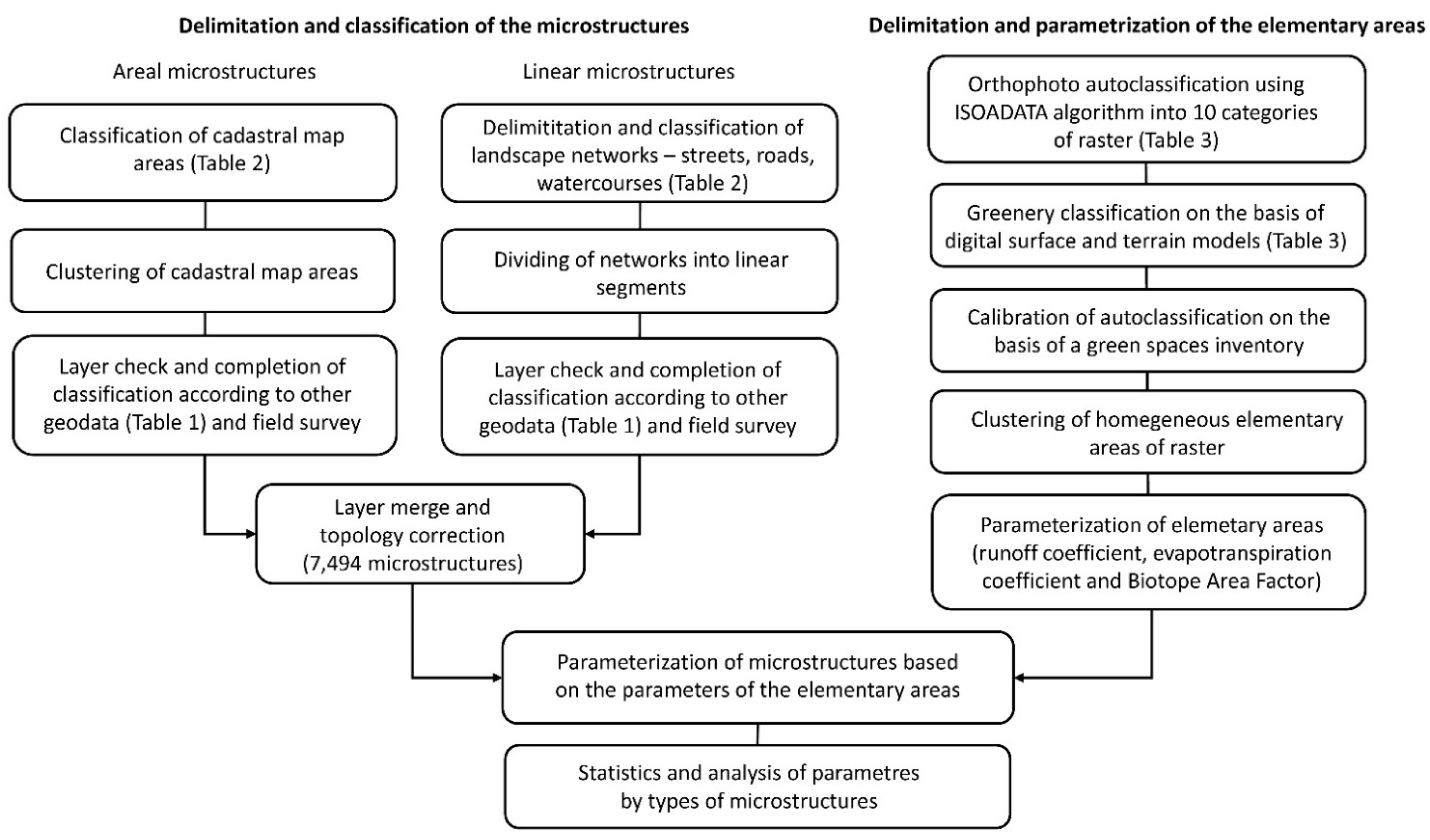
In the methodological part of the paper, the ecohydrological zoning of the urban landscape, which was created in GIS as a basis for planning the blue-green infrastructure of cities in the Czech Republic, is presented. The essence of the methodology is a two-level categorization of territorial units, which is based on the possibility to determine some ecohydrological parameters at various levels of detail. The resulting ecohydrological zoning of the city of Pilsen and parameterization at the level of microstructures was compared with the zoning of the city by a standardized procedure for defining LCZ. The resulting evaluation of raster cells of individual LCZ classes according to ecohydrological parameters must be considered as a case study, the generalization of which is limited. The limit of generalization is both the specific characteristics of the urban landscape of Pilsen and also own procedure of ecohydrological zoning, based on available data sets for the city. The comparison of methodological procedures for the definition of LCZ and zoning of ecohydrological microstructures with parameterization based on elementary areas results in a different level of scale for distinguishing the characteristics of the urban landscape. Standardized procedures for delimiting LCZ are aimed at defining larger territorial units of the same morphology of built-up areas and land cover in a grid scale of 100 × 100 m. A more universal use of the LCZ classification would be helped by the choice of more detailed data and the resulting scale of spatial units [25,26], or a link to territorial units of administrative-functional use [29]. For practical application of the results is more suitable, when units delimited as urban blocks according to type of built-up area are used for the assessment of the territory on the basis of LCZ [27]. On the other hand, the standardization of procedures is limited by the fact that LCZ categorization is applied worldwide in different climatic zones with different urban development.

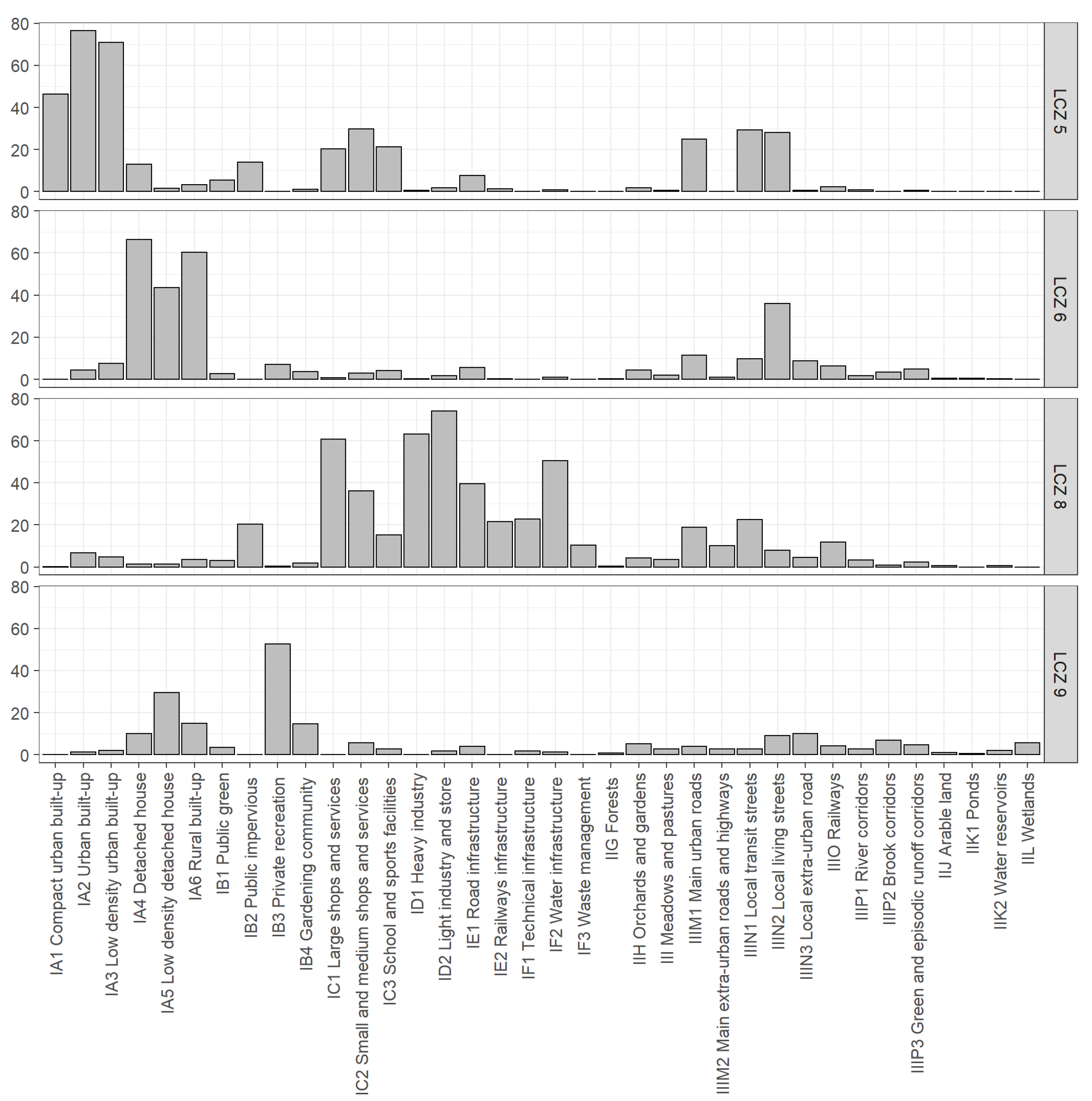
Defining and parameterizing the ecohydrological properties of microstructures purposefully takes into account the functional use of areas and the slope of the area, seeking to distinguish elementary areas up to a grid level of 0.5 m. However, the process of defining microstructures has not been fully automated and the accuracy of the resolution depends on the underlying data, such as the availability and quality of the urban green spaces inventory. Based on the zoning of the area into ecohydrological microstructures, adaptation measures can be better spatially targeted, for example thanks to a separate assessment of street corridors. Despite the mentioned differences in climatological and ecohydrological zoning, it was proved on the example of the territory of the city of Pilsen that both zonations correspond to a certain extent. In other words, the defined LCZ classes show different ecohydrological properties.

However, the presented statistical description of both zonings of the area cannot prove a detailed dependence of climatic and ecohydrological properties for two reasons: it is not based on direct measurements and cannot take into account detailed differences within units. For example, the categorization of buildings does not take into account the occurrence of green roofs and facades, which may affect the outflow or evapotranspiration [35]. However, this must be demonstrated by detailed research and measurements on individual surfaces in different microclimatic position [10,62].

The zoning of the area according to LCZ is, of course, too rough to capture the microclimatic differences affected by the detailed parameterization of street corridors, buildings and individual surfaces of the city in the horizontal and vertical scale. The used ecohydrological classification is also unable to distinguish some details of the area, e.g., greenery leaf size (leaf area index), green roofs hydration degree [35], but it showed the possibilities of supplementing the structure of data on individual areas of LCZ, so that they are more generally applicable for the evaluation of the potential of BGI of the city.

The determined distribution of the level of runoff, evapotranspiration and BAF coefficients in the territory of Pilsen mainly corresponds to the share of permeable and impervious areas, which is one of the standardized parameters defining the types of LCZ. The permeability parameters of the areas mediate a significant link to other properties of the area—the potential distribution of infiltration, runoff and evaporation of rainwater. Results confirm that types of residential areas are significantly associated with some types of ecosystem service [63].

The links between water circulation and climatic parameters are demonstrated on the basis of modeling the energy significance of the evapotranspiration process [40,41,42]. However, less attention is paid to runoff links, although this is a more measurable component of the hydrological balance. The inclination of the area as an important parameter of runoff is distinguished. Climatological zonations take it into account only in the case of the effect on exposure to solar radiation.

There is currently a discussion about the possible extension of the LCZ classification to aspects of forms of urban landscape relief, which are described as part of non-urban effects. The proposed combination of LCZ types and orographic classification of urban sites is driven by an effort to better capture the topoclimatic conditions in the hilly relief in some cities. The use of the classification of relief forms could thus support a holistic expression of the characteristics of the urban landscape [64], also taking into account runoff conditions. However, a more accurate distinction of the slope of the area is more important for determining the runoff conditions.

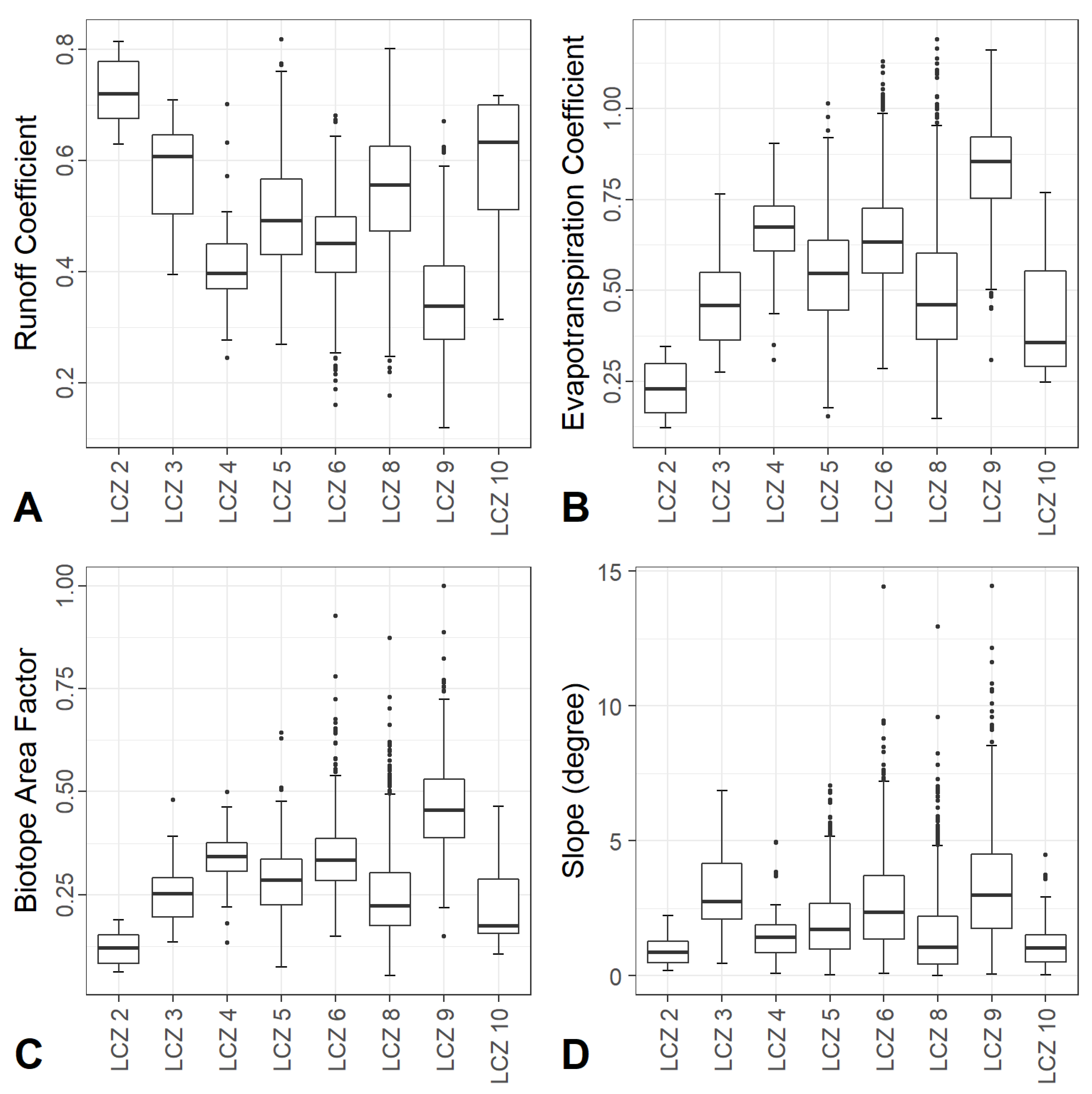
As our analysis of the inclination of the area according to the types of LCZ on the example of Pilsen has shown, there are differences between the individual types (

Table 6. Statistics of LCZ cells according to slope parametrization.

LCZ	LCZ 2	LCZ 3	LCZ 4	LCZ 5	LCZ 6	LCZ 8	LCZ 9	LCZ 10
N	41	35	38	887	959	1267	562	52
Mean	0.9571	3.2275	1.6581	1.9319	2.6994	1.5425	3.3630	1.2814
Median	0.8716	2.7713	1.4485	1.7180	2.3654	1.0604	3.0009	1.0367
Min	0.1857	0.4522	0.0806	0.0502	0.0897	0.0165	0.0730	0.0397
Max	2.2292	6.8566	4.9525	7.0350	14.4265	12.9549	14.4487	4.4768
Var	0.2957	2.5864	1.4618	1.5546	3.0368	2.1303	4.7662	1.2275
SD	0.5438	1.6082	1.2091	1.2468	1.7426	1.4595	2.1832	1.1079
CV	56.8190	49.8297	72.9162	64.5388	64.5551	94.6226	64.9177	86.4611

Note: N—number of LCZ cells, Min—minimum, Max—maximum, Var—variance, SD—standard deviation, CV—coefficient of variation.

, Figure 6). There is also a large variance of values for LCZ 6, 8 and 9. However, these differences do not explain the level of distribution of the runoff coefficient in individual LCZ. LCZ with higher values of inclination (LCZ 9, LCZ 6) represent the area of detached houses, which can be situated with their gardens on the slopes of river valleys, etc. However, this character of the urban landscape with the representation of greenery generally shows lower values of runoff than flat areas built up by large buildings of industrial, trade and services (LCZ 8) or modernist high-rise apartment buildings (LCZ 5). The assumption that the area of LCZ 8 needs to be addressed as a priority not only from the point of view of thermal overheating [65], but also from the point of view of ecohydrology, was confirmed. These areas also show unfavorably high values of surface runoff. Moreover, in the case of Pilsen, LCZ 8 has a significant representation in some sectors of the inner city, where industrial zones extend [45]. To discuss the effect of inclination, it should be added that this parameter has no additional effect on the parameterization of runoff for impervious surfaces, because the standards assign a level of coefficient 1 regardless of the inclination of the area.

Impermeability of areas and lack of greenery in the built-up area, typically in the microstructures of production and storage areas, classified mainly in LCZ 8, are essential for the risk of extreme runoff events. In this case, it is confirmed that the delimitation of LCZ in cities can be used to plan not only the mitigation of thermal stress, but also to more comprehensive planning of adaptation measures. However, it is appropriate to supplement the zoning of LCZ at a more detailed level with other parameters of the area important for BGI planning (e.g., slope of the area, possibilities of water retention in the area or risk of pollution of direct runoff).

Other links between LCZ typology and ecohydrological zoning exist through parameters such as e.g., surface covered by high vegetation, surface covered by low vegetation [61]. In the territory of Pilsen, differences in the level of ecosystem services of individual city zones classified according to LCZ were proved via BAF indicator. In the detail of individual plots or functional microstructures, it is possible to develop the use of complex BGI indexes, such as biotope area factor. However, complex indicators should not only take into account rainwater management, but also other ecosystem services, including the level of microclimatic effects of the area.

In this case, it is possible to explain the variability of the values of ecohydrological parameters of individual types of LCZ by the required accuracy of the resolution of both zonations and the accuracy of the used data on the territory. However, more general conclusions can be made after testing in a larger number of cities, because the results may be affected by the specific structure of the territory and the development of built-up areas in the city of Pilsen. More detailed research and verification of links in other cities [34] can thus be a way to generalize the parameterization of LCZ to the level of expression of other ecosystem services, such as water retention, impact on health, air quality, etc. The result could be a comprehensive zoning system of the city as a basis for environmental modeling, including not only climatic aspects, but also runoff conditions, the possibility of solar energy production or effects on air quality [14].

5. Conclusions

The presented study brings new findings in three fields: (1) it compares methodological approaches to ecohydrological and climatological zoning of the cities, (2) it records the ecohydrological properties of the areas of individual LCZ classes in the model area, (3) it discusses the possibilities of supplementing the classification parameters of LCZ with other aspects, especially the slope of the territory.

(1) A comparison of two approaches to the zoning of the territory of the city of Pilsen has shown that it is possible to seek a connection between methodological approaches based on research in both climatology and ecohydrology. Based on the presented case study, it is possible to recommend further verification of the links between climatic and ecohydrological processes in the city, both towards the generalization of knowledge for Central European cities and towards standardization of data sources and their effective processing for city management.

(2) The direct connection of climatological and ecohydrological properties of the area is enabled by common parameters such as permeability of areas or the degree of greenery. A significant difference factor between the properties defining LCZ and the parameters of ecohydrological microstructures is the slope of the area, influencing the degree of surface runoff. In the territory of Pilsen, however, it turned out that the slope of the territory is not an explanatory factor of differences in the runoff coefficient in the built-up areas between LCZ classes.

(3) The results indirectly show that the slope of the area is related to the spatial distribution of LCZ types. This could be developed when defining orographic subtypes of LCZ for use at least in Central European conditions. This direction of supplementing the LCZ classification with non-urban effects will help a holistic approach to the classification of the urban landscape.

Further unification of approaches for the processing of analytical maps will be beneficial for the practice of cities in the field of adaptive measures to climate change, because it is also appropriate to unify tools of adaptation and look for the synergistic effects of BGI planning.

References

1. Kabisch, N.; Korn, H.; Stadler, J.; Bonn, A. Nature-Based Solutions to Climate Change Adaptation in Urban. Areas—Linkages between Science, Policy and Practice; Theory and Practice of Urban Sustainability Transitions; Springer Open: Cham, Switzerland, 2017. [Google Scholar]
2. Wong, T.H.F.; Brown, R. The water sensitive city: Principles for practice. Water Sci. Technol. 2009, 60, 673–682. [Google Scholar] [CrossRef] [PubMed] [Green Version]
3. Bokwa, A.; Dobrovolný, P.; Gál, T.; Geletič, J.; Gulyás, Á.; Hajto, M.J.; Holec, J.; Hollósi, B.; KielarI, R.; Lehnert, M.; et al. Urban Climate in Central European Cities and Global climate change. Acta Climatol. 2018, 51–52, 7–35. [Google Scholar] [CrossRef]
4. Stewart, I.D. A systematic review and scientific critique of methodology in modern urban heat island literature. Int. J. Clim. 2011, 31, 200–217. [Google Scholar] [CrossRef]
5. Zölch, T.; Maderspacher, J.; Wamsler, C.; Pauleit, S. Using green infrastructure for urban climate-proofing: An evaluation of heat mitigation measures at the micro-scale. Urban. For. Urban. Green. 2016, 20, 305–316. [Google Scholar] [CrossRef]
6. Hoang, L.; Fenner, R.A. System interactions of stormwater management using sustainable urban drainage systems and green infrastructure. Urban. Water J. 2016, 13, 739–758. [Google Scholar] [CrossRef] [Green Version]
7. Voskamp, I.M.; van de Ven, F.H.M. Planning support system for climate adaptation: Composing effective sets of blue-green measures to reduce urban vulnerability to extreme weather events. Build. Environ. 2015, 83, 159–167. [Google Scholar] [CrossRef]
8. Howe, C.; Mitchell, C. (Eds.) Water Sensitive Cities; IWA Publishing: London, UK, 2012. [Google Scholar]
9. Woods Ballard, B.; Wilson, S.; Udale-Clarke, H.; Illman, S.; Scott, T.; Ashley, R.; Kellagher, R. The SUDS Manual (C753). CIRIA: London, UK, 2015. [Google Scholar]
10. DiGiovanni-White, K.; Montalto, F.; Gaffin, S. A comparative analysis of micrometeorological determinants of evapotranspiration rates within a heterogeneous urban environment. J. Hydrol. 2018, 562, 223–243. [Google Scholar] [CrossRef]
11. Lehnert, M.; Tokar, V.; Jurek, M.; Geletič, J. Summer thermal comfort in Czech cities: Measured effects of blue and green features in city centres. Int. J. Biometeorol. 2020, 1–13. [Google Scholar] [CrossRef]
12. Žuvela-Aloise, M.; Koch, R.; Buchholz, S.; Früh, B. Modelling the potential of green and blue infrastructure to reduce urban heat load in the city of Vienna. Clim. Chang. 2016, 135, 425–438. [Google Scholar] [CrossRef] [Green Version]
13. Norton, B.A.; Coutts, A.M.; Livesley, S.J.; Harris, R.J.; Hunter, A.M.; Williams, N.S.G. Planning for cooler cities: A framework to prioritise green infrastructure to mitigate high temperatures in urban landscapes. Landsc. Urban. Plan. 2015, 134, 127–138. [Google Scholar] [CrossRef]
14. Lindberg, F.; Grimmond, C.S.B.; Gabey, A.; Huang, B.; Kent, C.H.W.; Sun, T.; Theeuwes, N.E.; Järvi, L.; Ward, H.C.; Capel-Timms, I.; et al. Urban Multi-scale Environmental Predictor (UMEP): An integrated tool for city-based climate services. Environ. Model. Softw. 2018, 99, 70–87. [Google Scholar] [CrossRef]
15. Järvi, L.; Grimmond, C.S.B.; Christen, A. The Surface Urban Energy and Water Balance Scheme (SUEWS): Evaluation in Los Angeles and Vancouver. J. Hydrol. 2011, 411, 219–237. [Google Scholar] [CrossRef]
16. Perini, K.; Sabbion, P. Urban Sustainability and River Restoration, Green and Blue Infrastructure Sensitive Cities; WILEY Blackwell: Chichester, UK, 2017. [Google Scholar]
17. Thorne, C. (Ed.) Delivering and Evaluating Multiple Flood Risk Benefits in Blue-Green Cities; Key Project Outputs. EPSRC Project EP/K013661/1; University of Nottingham: Nottingham, UK, 2016. [Google Scholar]
18. Bacchin, T.; Ashley, R.; Blecken, G.; Viklander, M.; Gersonius, B. Green-blue Infrastructure for Sustainable Cities: Innovative Socio-technical Solutions Bringing Multifunctional Value. In Proceedings of the Novatech, 9th International Conference on Planning and Technologies for Sustainable URBAN WATER Management, Lyon, France, 28 June–1 July 2016; pp. 1–4. [Google Scholar]
19. Kopp, J.; Preis, J. The potential implementation of stormwater retention ponds into the blue-green infrastructure of the suburban landscape of Pilsen, Czechia. Appl. Ecol. Environ. Res. 2019, 17, 15055–15072. [Google Scholar] [CrossRef]
20. Alves, A.; Vojinovic, Z.; Kapelan, Z.; Sanchez, A.; Gersonius, B. Exploring trade-offs among the multiple benefits of green-blue-grey infrastructure for urban flood mitigation. Sci. Total Environ. 2020, 703, 134980. [Google Scholar] [CrossRef] [PubMed]
21. McPhearson, T.; Depietri, Y. Integrating the Grey, Green, and Blue in Cities: Nature-Based Solutions for Climate Change Adaptation and Risk Reduction. In Nature-Based Solutions to Climate Change Adaptation in Urban Areas. Linkages between Science, Policy and Practice; Kabisch, N., Korn, H., Stadler, J., Bonn, A., Eds.; Springer Open: Cham, Switzerland, 2017; pp. 91–109. [Google Scholar]
22. Alexander, P.J.; Mills, G. Local Climate Classification and Dublin’s Urban Heat Island. Atmosphere 2014, 5, 755–774. [Google Scholar] [CrossRef] [Green Version]
23. Stewart, I.D.; Oke, T.R. A new classification system for urban climate sites. Bull. Am. Meteorol. Soc. 2009, 90, 922–923. [Google Scholar]
24. Stewart, I.D.; Oke, T.R. Local Climate Zones for Urban Temperature Studies. Bull. Amer. Meteor. Soc. 2012, 93, 1879–1900. [Google Scholar] [CrossRef]
25. Richard, Y.; Emery, J.; Dudek, J.; Pergaud, J.; Chateau-Smith, C.; Zito, S.; Rega, M.; Vairet, T.; Castel, T.; Thévenin, T.; et al. How relevant are local climate zones and urban climate zones for urban climate research? Dijon (France) as a case study. Urban. Clim. 2018, 26, 258–274. [Google Scholar] [CrossRef] [Green Version]
26. Verdonck, M.-L.; Okujeni, A.; van der Linden, S.; Demuzere, M.; De Wulf, R.; van Coillie, F. Influence of neighbourhood information on ‘Local Climate Zone’ mapping in heterogeneous cities. Int. J. Appl. Earth Obs. Geoinf. 2017, 62, 102–113. [Google Scholar] [CrossRef]
27. Quan, S.J.; Bansal, P. A systematic review of GIS-based local climate zone mapping studies. Build. Environ. 2021, 196, 107791. [Google Scholar] [CrossRef]
28. Lehnert, M.; Savić, S.; Milošević, D.; Dunjić, J.; Geletič, J. Mapping Local Climate Zones and Their Applications in European Urban Environments: A Systematic Literature Review and Future Development Trends. ISPRS Int. J. Geo-Inf. 2021, 10, 260. [Google Scholar] [CrossRef]
29. Hidalgo, J.; Dumas, G.; Masson, V.; Petit, G.; Bechtel, B.; Bocher, E.; Foley, M.; Schoetter, R.; Mills, G. Comparison between local climate zones maps derived from administrative datasets and satellite observations. Urban. Clim. 2019, 27, 64–89. [Google Scholar] [CrossRef] [Green Version]
30. Lehnert, M.; Geletič, J.; Husák, J.; Vysoudil, M. Urban field classification by “local climate zones” in a medium-sized Central European city: The case of Olomouc (Czech Republic). Appl. Climatol. 2015, 122, 531–541. [Google Scholar] [CrossRef]
31. Müller, N.; Kuttler, W.; Barlag, A.B. Counteracting urban climate change: Adaptation measures and their effect on thermal comfort. Appl. Climatol. 2014, 115, 243–257. [Google Scholar] [CrossRef] [Green Version]
32. Leconte, F.; Bouyer, J.; Claverie, R. Nocturnal cooling in Local Climate Zone: Statistical approach using mobile measurements. Urban. Clim. 2020, 33, 100629. [Google Scholar] [CrossRef]
33. Xue, J.; You, R.; Liu, W.; Chen, C.; Lai, D. Applications of Local Climate Zone Classification Scheme to Improve Urban Sustainability: A Bibliometric Review. Sustainability 2020, 12, 8083. [Google Scholar] [CrossRef]
34. Das, M.; Das, A. Estimation of Ecosystem Services (EESs) loss due to transformation of Local Climatic Zones (LCZs) in Sriniketan-Santiniketan Planning Area (SSPA) West Bengal, India. Sustain. Cities Soc. 2019, 47, 101474. [Google Scholar] [CrossRef]
35. Antoszewski, P.; Świerk, D.; Krzyżaniak, M. Statistical Review of Quality Parameters of Blue-Green Infrastructure Elements Important in Mitigating the Effect of the Urban Heat Island in the Temperate Climate (C) Zone. Int. J. Environ. Res. Public Health 2020, 17, 7093. [Google Scholar] [CrossRef]
36. Wagner, I.; Breil, P. The role of ecohydrology in creating more resilient cities. Ecohydrol. Hydrobiol. 2013, 13, 113–134. [Google Scholar] [CrossRef]
37. Lafortezza, R.; Chen, J.; van den Bosch, C.K.; Randrup, T.B. Nature-based solutions for resilient landscapes and cities. Environ. Res. 2018, 165, 431–441. [Google Scholar] [CrossRef]
38. Bozovic, R.; Maksimovic, C.; Mijic, A.; Smith, K.M.; Suter, I.; van Reeuwijk, M. Blue Green Solutions. A Systems Approach to Sustainable, Resilient and Cost-Efficient Urban Development; Climate-KIC Limited, Imperial College London: London, UK, 2017. [Google Scholar]
39. Alexander, P.J.; Mills, G.; Fealy, R. Using LCZ data to run an urban energy balance model. Urban. Clim. 2015, 13, 14–37. [Google Scholar] [CrossRef] [Green Version]
40. Mitchell, V.G.; Cleugh, H.A.; Grimmond, C.S.B.; Xu, J. Linking urban water balance and energy balance models to analyse urban design options. Hydrol. Process. 2008, 22, 2891–2900. [Google Scholar] [CrossRef]
41. Xiao, Q.; McPherson, E.G.; Simpson, J.R.; Ustin, S.L. Hydrologic processes at the urban residential scale. Hydrol. Process. 2007, 21, 2174–2188. [Google Scholar] [CrossRef]
42. Omidvar, H.; Sun, T.; Grimmond, S.; Bilesbach, D.; Black, A.; Chen, J.; Duan, Z.; Gao, Z.; Iwata, H.; McFadden, J.P. Surface [Urban] Energy and Water Balance Scheme (v2020a) in non-urban areas: Developments, parameters and performance. Geosci. Model. Dev. Discuss. 2020. [Google Scholar] [CrossRef]
43. Aubrechtová, T.; Geletič, J.; Lehnert, M. Identifikace Lokalit Ohrožených Teplotním Stresem—Nástroj Pro Udržitelné Plánování Měst (Identification of Locations Vulnerable to Thermal Stress—A Tool for Sustainable Urban Planning); Project No. TJ01000118. Project Final Report; Global Change Research Institute of the Czech Academy of Sciences: Brno, Czech Republic; Palacký University Olomouc: Olomouc, Czech Republic, 2019. (In Czech) [Google Scholar]
44. Vít, V.; Kopp, J. Typology of Outdoor Seating Areas of Restaurants Based on Factors Influencing Their Thermal Comfort. A Case Study of Pilsen City Centre, Czechia. J. Settl. Spat. Plan. 2019, 10, 131–142. [Google Scholar]
45. Kopp, J.; Raška, P.; Vysoudil, M.; Ježek, J.; Dolejš, M.; Veith, T.; Frajer, J.; Novotná, M.; Hašová, E. Ekohydrologický Management Mikrostruktur Městské Krajiny (Ecohydrological Management of the Urban Landscape´s Microstructures); Západočeská univerzita v Plzni: Plzeň, Czech Republic, 2017. (In Czech) [Google Scholar]
46. Pauleit, S.; Duhme, F. Assessing the environmental performance of land cover types for urban planning. Landsc. Urban. Plan. 2000, 52, 1–20. [Google Scholar] [CrossRef]
47. Derkzen, M.L.; van Teeffelen, A.J.A.; Verburg, P.H. Quantifying urban ecosystem services based on high-resolution data of urban green space: An assessment for Rotterdam, The Netherlands. J. Appl. Ecol. 2015, 52, 1020–1032. [Google Scholar] [CrossRef]
48. Sulzer, W. Reale Abbildung der Stadtentwicklung Graz—Landnutzungskartierung 1945–2015; Eigenverlag der Stadt Graz: Graz, Austria, 2016. [Google Scholar]
49. Zonneveld, I.S. The land unit—A fundamental concept in landscape ecology, and its applications. Landsc. Ecol. 1989, 3, 67–86. [Google Scholar] [CrossRef]
50. Faltermaier, M.; Stock, H.; Tonndorf, T. (Eds.) Stadtentwicklungsplan Klima KONKRET Klimaanpassung in der Wachsenden Stadt; Senatsverwaltung für Stadtentwicklung und Umwelt: Berlin, Germany, 2016. [Google Scholar]
51. Kazmierczak, A.; Carter, J. Adaptation to Climate Change Using Green and Blue Infrastructure. A Database of Case Studies; University of Manchester: Manchester, UK, 2010. [Google Scholar]
52. Allen, R.G.; Pereira, L.S.; Raes, D.; Smith, M. Crop. Evapotranspiration—Guidelines 157 for Computing Water Requirements; Irrigation and Drainage Paper No. 56; FAO: Rome, Italy, 1998. [Google Scholar]
53. Costello, L.R.; Matheny, N.P.; Clark, J.R.; Jones, K.S. A Guide to Estimating Irrigation Water Needs of Landscape Plantings in California. The Landscape Coefficient Method and WUCOLS III; University of California Cooperative Extension; California Department of Water Resources: Sacramento, CA, USA, 2000. [Google Scholar]
54. Kjelgren, R.; Beeson, R.C.; Pittenger, D.R.; Montague, D.T. Simplified landscape irrigation demand estimation: Slide rules. Appl. Eng. Agric. 2016, 32, 363–378. [Google Scholar] [CrossRef]
55. Lehnert, M.; Geletič, J.; Dobrovolný, P.; Jurek, M. Temperature differences among local climate zones established by mobile measurements in two central European cities. Clim. Res. 2018, 75, 53–64. [Google Scholar] [CrossRef]
56. Developing the City of Helsinki Green Factor Method. Report Summary; City of Helsinki, Environment Centre Helsinki: Helsinki, Finland, 2016.
57. Handlungsziele für Stadtgrün und Deren Empirische Evidenz. Indikatoren, Kenn- und Orientierungswerte; Bundesinstitut für Bau-, Stadt- und Raumforschung: Bonn, Germany, 2018.
58. Peroni, F.; Pristeri, G.; Codato, D.; Pappalardo, S.E.; De Marchi, M. Biotope Area Factor: An Ecological Urban Index to Geovisualize Soil Sealing in Padua, Italy. Sustainability 2020, 12, 150. [Google Scholar] [CrossRef] [Green Version]
59. Becker, C.W. (Ed.) The Biotope Area Factor as an Ecological Parameter. Principles for Its Determination and Identification of the Target; Becker Giseke Mohren Richard, Landschaft Planen & Bauen: Berlin, Germany, 1990. [Google Scholar]
60. Stewart, I.D.; Oke, T.R.; Krayenhoff, E.S. Evaluation of the ‘local climate zone’ scheme using temperature observations and model simulations. Int. J. Climatol. 2014, 34, 1062–1080. [Google Scholar] [CrossRef]
61. Geletič, J.; Lehnert, M. GIS-based delineation of local climate zones: The case of medium-sized Central European cities. Morav. Geogr. Rep. 2016, 24, 2–12. [Google Scholar] [CrossRef] [Green Version]
62. Lehnert, M.; Brabec, M.; Jurek, M.; Tokar, V.; Geletič, J. The role of blue and green infrastructure in thermal sensation in public urban areas: A case study of summer days in four Czech cities. Sustain. Cities Soc. 2021, 66, 102683. [Google Scholar] [CrossRef]
63. Tratalos, J.; Fuller, R.A.; Warren, P.H.; Davies, R.G.; Gaston, K.J. Urban form, biodiversity potential and ecosystem services. Landsc. Urban. Plan. 2007, 83, 308–317. [Google Scholar] [CrossRef]
64. Stewart, I.D. Developing a field guide to identify ‘local climate zones’ in cities. In Proceedings of the 10th International Conference on Urban Climate/14th Symposium on the Urban Environment, New York, NY, USA, 6–10 August 2018. Abstract 12E.1. [Google Scholar]
65. Geletič, J.; Lehnert, M.; Savić, S.; Milošević, D. Modelled spatiotemporal variability of outdoor thermal comfort in local climate zones of the city of Brno, Czech Republic. Sci. Total Environ. 2018, 624, 385–395. [Google Scholar] [CrossRef]
Figure 1. Geographical conditions of the territory of the city of Pilsen. Data sources: ArcČR500 (2016); Czech Office for Surveying, Mapping and Cadaster (2020); Openstreet maps and Geofabrik (2020).
Ijgi 10 00350 g001
Figure 2. Flow-chart of the ecohydrological zoning of the city of Pilsen.
Ijgi 10 00350 g002
Figure 3. Delimiting local climate zones (LCZ) in the cadastral area of Pilsen. Source: own processing based on classification algorithm [61].
Ijgi 10 00350 g003
Figure 4. Ecohydrological parameterization of LCZ raster on the basis of microstructures.
Ijgi 10 00350 g004
Figure 5. Relative representation of microstructure types in LCZ 5–LCZ 9 (%).
Ijgi 10 00350 g005
Figure 6. Box plots of LCZ classes according to ecohydrological parameters ((A) runoff coefficient, (B) evapotranspiration coefficient, (C) biotope area factor) and slope (D). The lower part of the box is the first quartile, and the upper is the third quartile. Whiskers indicate the lowest value still within 1.5 IQR (IQR = third quartile−first quartile) and the highest value still within 1.5 IQR. Points indicate outliers.
Ijgi 10 00350 g006
Figure 7. Distributions of LCZ 5–LCZ 9 cells according to ecohydrological parameters ((A) runoff coefficient, (B) evapotranspiration coefficient, (C) biotope area factor).
Ijgi 10 00350 g007