Usage of Airborne Hyperspectral Imaging Data for Identifying Spatial Variability of Soil Nitrogen Content

Abstract

Soil is a significant natural resource composed of organic and inorganic material. Nitrogen, one of the essential elements, is traditionally measured using laboratory methods. The development of hyperspectral imaging enables the cost-effective acquisition of both spectral and spatial information for detecting physical, chemical, and biological attributes of the soil samples. The presented work evaluates the suitability of airborne hyperspectral imaging for determining soil nitrogen content and producing a soil nitrogen map on a pixel-wise basis. The measurement of spatial variability of the soil nitrogen content was taken at two fields located at Rudice, in northeast Brno, Czech Republic, using laboratory methods and a handheld spectrometer. The soil reflectance was also recorded using airborne-mounted imaging spectroscopy sensors. A partial least squares regression was used to develop a model for the calibration of the data collected with a portable spectrometer and to predict the total nitrogen in the soils based on hyperspectral images from airborne sensors. The determination factor for the PLSR model presented in this paper reached an R² of 0.44. The model’s performance could be improved by using a handheld spectrometer with a wider spectral range, using the same acquisition period for field data collection and hyperspectral imaging, and enlarging the sample size.

1. Introduction

Soil is a fundamental natural non-renewable resource that people rely on for food production, fiber, and energy. It is also a habitat for microorganisms and earthworms and the foundation for buildings and other constructions [1]. Fundamentally, soil is a complex matrix that consists of organic and inorganic mineral matter, water, and air. The organic material in soils ranges from decomposed and stable humus to fresh, particulate residues of various origins. The distribution of these different organic pools in soil influences biological activity, nutrient availability and its dynamics, soil structure and aggregation, and water-holding capacity [2]. The inorganic mineral fractions are often described by their particle size distribution (proportions of sand, silt, and clay) and by additional subclasses in various classification systems [3]. Nitrogen (N) is one of the essential elements that affect vegetative growth and plant development because it plays a central role in all metabolic processes, as well as in cellular structure and genetic coding [4]. Its association with phosphorus (P) plays a vital role in plant growth as these two elements interact with each other. Therefore, it is essential to investigate the N content in the soils and obtain the spatial distribution information that would improve field nitrogen management efficiency and the economic benefit from agricultural production and contribute to sustainable agriculture [5].

The goal of the research was to determine the total soil nitrogen (Ntot); its concentration was expressed in the percentage of dry weight of soil (%). It consists of all accessible and inaccessible forms that can pass between each other. The natural nitrogen cycle depends on the ability of organisms to bind and convert inert atmospheric nitrogen (N₂) and decompose proteins. The basic mineral forms of ammonium (NH₄⁺) and nitrate (NO₃^–) are also important accessible forms of nitrogen for plant nutrition and indication of soil viability. Both forms of nitrogen move in the soil sorption complex, indicating the degree of eutrophication and the efficiency of the nitrogen cycle.

The nitrogen content in the soils is usually measured using laboratory methods. However, they are often time consuming, expensive, and destructive. Therefore, new techniques such as laboratory spectroscopy are being developed to minimize the disadvantage of traditional laboratory methods [6]. Examples of popular spectrometers include ASD FieldSpec 3, Peristrom NIR System 6500, and FOSS XSD Rapid Content Analyzer Spectrometer [5,7,8,9]. These devices measure mostly at spectral bandwidths ranging from 1 to 2 nm over a wavelength range of 300 to 2500 nm.

Another option is to use remote sensing methods. There are aerial and satellite remote sensing techniques. Aerial remote sensing is generally used to acquire data for smaller areas (national scale), while satellite remote sensing is used for covering larger areas (global scale). In addition, there are three types of optical data. The first is panchromatic, which is characterized by high or very high spatial resolution and a single band. The band is formed by total light energy in a visible spectrum. Multispectral data have a higher spectral resolution consisting of multiple spectral bands with broader bandwidth instead of lower spatial resolution compared to panchromatic data. Therefore, a pan-sharpening method is sometimes employed, which improves the spatial resolution of multispectral data. For example, Sentinel-2A has 13 spectral bands in visible, NIR (near-infrared), and SWIR (short-wavelength infrared) spectra with a spatial resolution of 10, 20, and 60 meters, respectively. The range of bandwidth is from 15 to 175 nm [10]. Hyperspectral data contain many spectral bands compared to multispectral data. However, their main advantage is contiguous bands with narrow bandwidth. As a result, the spectral curve of a surface is continuous. Hyperspectral images are used for soil mapping [11] or identifying types of iron and clay minerals [12].

Aerial and satellite hyperspectral images enable the mapping of relatively large areas over a short period. However, the raw data must be corrected to eliminate the influence of the atmosphere in the determination of soil properties [13]. Hyperspectral imaging combines conventional spectroscopy with imaging techniques to acquire spectral and spatial information to detect physical, chemical, and biological attributes of the samples [14,15]. A soil spectrum is generated by directing radiation containing all relevant frequencies to the sample. Depending on the constituents present in the soil, the radiation will cause individual molecular bonds to vibrate, either by bending or stretching, and absorb light to various degrees. The resulting absorption spectrum produces a characteristic shape that can be used for analytical purposes [16]. Visible and near-infrared (vis–NIR) regions, encompassing wavelengths between 400 and 2500 nm, contain useful information on organic and inorganic materials in the soil. Absorptions in these regions can be used to detect mineral content associated with iron, soil organic matter, clay, carbonates, or water [17,18,19,20]. It can also be used to detect soil matter, such as organic carbon (SOC) or total nitrogen, as a result of the stretching and bending of NH, CH, and CO groups [21,22,23,24,25]. Viscarra Rossel and Behrens [26] present a summary of important fundamental absorptions in the mid-infrared (mid-IR) region and the occurrence of their overtones and combinations in the vis–NIR regions, which can be used to help with the interpretation of soil constituents.

Diffuse reflectance spectra of soil in the vis–NIR regions is largely nonspecific due to the overlapping absorption of soil constituents. This inherent lack of specificity is compounded by scattering effects caused by soil structure or its specific components such as quartz. All these factors result in complex absorption patterns that need to be mathematically extracted from the spectra and correlated with soil properties. Hence, the analyses of soil diffuse reflectance spectra require a sophisticated statistical technique to discern the response of the soil attributes from spectral characteristics [27]. The most common calibration methods for soil applications are based on linear regressions, namely, stepwise multiple linear regression (SMLR), principal component regression (PCR), and partial least squares regression (PLSR) [28]. The main reason for using SMLR is the inadequacy of more conventional regression techniques such as multiple linear regression (MLR) and the lack of awareness among soil scientists of the existence of full-spectrum data compression techniques such as PCR and PLSR. Both methods can cope with data containing large numbers of predictor variables that are highly collinear. PCR and PLSR are related techniques, and in most situations, their prediction errors are similar. However, PLSR is often preferred by analysts because it relates the response and predictor variables so that the model explains more of the variance in the response with fewer components, and the algorithm is therefore computationally faster. The use of data mining techniques such as neural networks (NN) [23,24], multivariate adaptive regression splines (MARS) [25] and boosted regression trees [26] is increasing. Viscarra Rossel et al. [29] combined PLSR with bootstrap aggregation (bagging-PLSR) to improve the robustness of the PLSR models and produce predictions with uncertainty. MLR, PCR, and PLS are linear models, while the data mining techniques can handle nonlinear data. Viscarra Rossel and Lark [28] used wavelets combined with polynomial regressions to reduce the spectral data, account for non-linearity, and produce accurate and parsimonious calibrations based on selected wavelet coefficients. Mouazen et al. [30] compared NN with PCR and PLS for predicting selected soil properties. They found combined PLSR-NN models to provide improved forecasts compared to PLSR and PCR. Viscarra Rossel and Behrens [26] examined the use of PLSR to several data mining algorithms and feature selection techniques for predictions of clay, organic carbon, and soil acidity (pH). The comparison included MARS, random forests (RF), boosted trees (BT), support vector machines (SVM), NN, and wavelet transform. Their results suggest that data mining algorithms produced more accurate results than PLSR. Some of the algorithms provide information on the importance of specific wavelengths in the models so that they can be used to interpret them.

The objectives of the presented study were to evaluate the suitability of airborne hyperspectral imaging, determine the soil nitrogen content, and produce a soil nitrogen map on a pixel-wise basis usable for precision agriculture. The goal was fulfilled with emphasis on the use of geoinformation technologies, for processing of hyperspectral data and performing spatial analyses in a GIS environment.

2. Materials and Methods

2.1. Study Site

The measurement of the spatial variability of the soil nitrogen content was taken at two fields located at Rudice, northeast Brno, Czech Republic (Figure 1). These sites were selected to provide soil samples from both agricultural land and grassland located near a forest. This region is characterized by mean annual precipitation of 393–430 mm and a mean annual temperature of approximately 8.3 °C. Due to the different soil cultivation, both test sites varied in surface roughness, soil structure, green coverage, and straw residue. At the agricultural test site, which has been under intensive cultivation, the soil surface was ploughed with residue coverage of less than 10%. According to the World Reference Base for Soil Resources [31], the dominant soil type of the test site is Luvisols.

Soil sampling and data collection with a portable spectrometer were performed on 10 October 2016. Due to unfavorable weather conditions on this day, the aerial imaging campaign was postponed and completed one month after the soil sampling. The soil was sampled from the top 5 cm of plough horizon at the agricultural site using core rings around randomly selected sampling points. The top 5 cm of soil horizon was discarded at the grassland field due to extensively dense root activity. Spatial coordinates were measured using handheld GPS. A total of 22 topsoil samples were collected from both sites.

2.2. Conventional Soil Analysis

The soil sampling and laboratory analysis were coordinated with the Institute of Geology and Soil Science, Mendel University in Brno. The presented study uses the results of analyses of soil samples taken from the soil horizon A1 at a depth of 5 cm. Before analysis, all soil samples were air-dried, passed through a 2 mm sieve, and milled before analysis. The total nitrogen was determined by a modified Kjeldahl method [32] that consists of a procedure of dissolving the soil samples in a boiling mixture of sulfuric acid and catalyst additives. The resulting NH₄+ ions together with the NH₄+ ions originally present in the sample after alkalization were distilled in the form of ammonia (NH₃) into a certain volume of a standard solution of sulfuric acid (H₂SO₄) as specified by the method. The captured NH₃ was then determined indirectly by the titration of the excess volumetric acid solution with a volumetric NaOH solution.

2.3. Field VIS/NIR Spectroscopy

The reflectance of the soil samples was measured in the field using the FieldSpec HandHeld2 portable spectrometer [33]. The HandHeld2 spectrometer offers a vis-NIR spectral range (325–1075 nm) with resolution better than 3 nm at 700 nm and accuracy of ±1 nm. A white Spectralon panel (approximately 10 cm in diameter) provided the absolute reflectance factor for field calibration of the device, and it was used before each sample measurement was taken. The distance between the scanned surface and the equipment was chosen so that the scanned area was approximately 30 cm × 30 cm. Three repeat measurements of soil spectrum were recorded per sample.

2.4. Hyperspectral Imaging in vis-NIR Range

The soil reflectance was recorded with the Flying Laboratory of Imaging Spectroscopy (FLIS). The flight campaign was conducted by CzechGlobe—Global Change Research Institute of the Czech Academy of Sciences (GCRI) on 8 November 2016. Weather conditions allowed imaging only early in the morning between 9 a.m. and 10 a.m. when the temperature ranged between −3 and 2 °C, as reported by a nearby meteorological measuring station located in Vranov. Due to the late data acquisition date, an increased noise level could be expected in the collected hyperspectral data, as reported by CzechGlobe. During the data collection, no rain occurred, and the precipitation rates for the prior five days were minimal, not exceeding 1 mm.

The FLIS consists of an aircraft-mounted set of three hyperspectral sensors from ITRES, Ltd. [34], two of which (CASI-1500 and SASI-600) collected data for the study. The CASI-1500 is a visible near-infrared (vis-NIR) sensor that offers 1500 pixels across its field of view, and a spectral range between 380 and 1500 nm with resolution better than 3.2 nm. The hyperspectral SASI-600 sensor captures 100 spectral channels across the shortwave infrared (SWIR) spectral region between 950 and 2450 nm with 600 across-track imaging pixels. The spatial pixel resolution for CASI-1500 and SASI-600 sensors is 1.5 m and 2.5 m, respectively, based on a 40-degree field of view and flight altitude of 2060 m. Radiometric calibration, an atmospheric correction, the exclusion of water absorption bands, and the georeferencing of the hyperspectral images were carried out by CzechGlobe to derive nadir normalized ground reflectance. Furthermore, as part of the pre-processing steps, the data from the two sensors were joined into the final hyperspectral image.

2.5. Partial Least Squares Regression (PLSR) Method

A partial least squares regression (PLSR) was used to develop a model for calibration of the data collected with FieldSpec HandHeld2 portable spectrometer with the reference soil nitrogen data from the laboratory analysis. Then, the PLSR was again applied to predict the total nitrogen content in the soils based on the developed model and data captured in the FLIS hyperspectral image. PLSR is a multi-linear regression technique that handles often strongly correlated spectral predictor bands well. This method reduces the dimensionality of the explanatory variables by projecting them into a certain number of new, orthogonal latent variables (LVs) [35]. PSLR transfers the information content of predictors to a few uncorrelated synthetic variables referred to as latent vectors. The latent vectors are generated not only with respect to maximizing information content regarding the spectral information but also due to their explanatory power in multiple linear regression. The optimization process involves the simultaneous implementation of dimensionality reduction and regression [36]. The developed PLSR models were calibrated by fitting them to the training data and validated by omitting one of the training points in the calibration phase and estimating the dependent variable for that point (Leave One Out, LOO, cross-validation). This method is based on sequentially removing one value from the dataset, testing the quality of the model’s prediction with the remaining values in the dataset, returning the removed value, and selecting another value that is removed from the dataset. The stability of the model was verified by predicting the total nitrogen content on the data with known values (validation set). The ratio of calibration and validation samples was 75% to 25%, respectively. Figure 2 shows the schematic process for predicting total nitrogen from hyperspectral images using the PLSR method.

Performance of the developed model was described using the coefficient of determination (R²) between measured and predicted values and root-mean-square error (RMSE) during the calibration and validation [37]. The optimal number of LVs is experimentally selected to minimize the determination coefficient during the calibration (R²cal), so model over-fitting is avoided and the determination coefficient during validation (R²val) is maximized [38].

2.6. Spectrometer Data Processing

Reflectance data collected with FieldSpec HandHeld2 portable spectrometer on 22 test sites were processed to remove the influence of the noise on the developed model. These marginal spectral range values vary from device to device. For FieldSpec HandHeld2, excessive noise was experimentally determined to affect the measured signal with a wavelength of less than 450 nm and greater than 950 nm, as shown in Figure 3. Nawi et al. [39] and Grant [40] also recommended removal of reflectance values in the wavelength range less than 600 nm and above 1000 nm and less than 450 nm and greater than 950 nm, respectively, to reduce the influence of the noise on measured data.

In the next step, the filtered spectral data were resampled to match the resolution and center wavelength value of the FLIS hyperspectral images recorded during the flight campaign. This step was accomplished using the freely available prospect package developed for the R environment [41]. The resampling process changed the original bandwidth width of the spectrometer’s data to about 14.2 nm and 15 nm to match the bandwidth width of the CASI and SASI sensor, respectively. This step further reduced the influence of the noise in the spectral data for model development. After noise removal and resampling, the reflectance data were transformed to absorbance using the following equation:

$$\mathrm{absorbance}={\log }_{10}\left(\frac{1}{\mathrm{reflectance}}\right)$$

(1)

2.7. Hyperspectral Data Processing

The FLIS hyperspectral image was imported into the R environment using the stack function of the raster package. However, the supplied hyperspectral image contained pixels with a value of 0 for the areas that were not imaged, as shown in the black color in Figure 4. Therefore, the values for 385,595 pixels, representing 36% of the hyperspectral image, were changed to “NoData” value.

After loading the FLIS hyperspectral image into the R environment, spectral bands that were not available in the resampled spectral information from the handheld spectrometer were removed. This step had to be performed because the hyperspectral image data on which the prediction itself was performed must have the same range and form as the data on which the model was built. This step led to the removal of SASI data with a wavelength of more than 1062.5 nm.

2.8. Model Development

The most critical step of the entire process was building the model, because the resulting values depend on the character of the model. Furthermore, the precision and accuracy of the prediction are dependent on the quality of input data, which often cannot be influenced, and on the quality of the developed model. Due to the relatively small size of the dataset (total of 22 samples), the standard procedure of dividing the entire dataset into the training set and validation set was not implemented, and the entire dataset was used to build the model. Validation of the developed model was performed using only the cross-validation method. During the model development, an iterative process of leave-one-out cross-validation was used. It sequentially hides one value from the dataset, tests the quality of its prediction with the remaining values, returns the value into the dataset, and then selects another value and hides it. Since the dataset was not extremely large, the model was built with a maximum number of latent variables. The PSLR function then calculated the RMSEP for the different number of latent variables, as seen in Figure 5.

The accepted recommendation for the selection of the number of latent components is based on displaying the RMSEP for a different number of latent components and then selecting one with the lowest RMSEP or from which RMSEP is not significantly reduced. Melvik and Wahrens [42] further refined this recommendation by claiming that it is preferable to select the number of components that display the first local root-mean-square error of prediction minimum, not the overall minimum. Based on the chart above, six components were chosen as RMSEP has the lowest value of 0.0178, while the model reached an R² of 0.45.

2.9. Prediction

For the prediction of soil nitrogen content, the PLSR library again employed FLIS hyperspectral image input, and the number of components was set to 6. The resulting predicted pixel values were then inserted into the original raster to maintain the identical geospatial structure. Before exporting the predicted total nitrogen content values, all but the first band were removed, as all the spectral bands contained the same predicted data. The matrix containing predicted total nitrogen content values was exported into TIF format in the final step.

2.10. Establishment of Bare Soil

The last step involved a process of removing pixels that do not logically correspond to the possible soil properties values and determining the bare soil to which the resulting data should correspond. The acquired raster for total nitrogen content also showed a certain number of negative values (

Table 1. Descriptive statistics for pixels with negative values.

Model	Number of Negative Pixels	Number of Negative Pixels (%)
N.abs	1255	0.17

N.abs = total nitrogen content in the soil (N), variant of the N model with the pre-treatment of the absorbance applied.

). This is logically impossible because the investigated quantities cannot have negative numbers. Therefore, these pixels were also removed to preserve only the portion of the raster with relevant data.

The mask for distinguishing pixels in the raster representing the bare soil was created using the normalized difference vegetation index (NDVI) and the cellulose absorption index (CAI). According to the authors of [43], this is one of the most reliable methods for determining the bare soil. To calculate the NDVI index from hyperspectral images, wavelengths of 800 nm for the NIR band, where the reflectivity of vegetation is increased, and 670 nm for the RED band were used [44]. The NDVI values in our area of interest ranged from −0.25 to 0.82. Negative values normally correspond to impermeable and artificial surfaces, such as roads or structures. Values approaching the value of 1 represent surfaces with a high chlorophyll content, such as dense green vegetation. Two masks were used to remove both extremes. Experimentally, it was determined that the first extreme included pixels with NDVI values ranging from −0.25 to 0.08 and the second one from 0.3 to 0.82.

The CAI index is used to determine the health status of vegetation based on the cellulose content. Gerighausen et al. [45] used the CAI index for detecting the arable land that was covered with vegetation. The index was developed for hyperspectral data and works with wavelengths of 2000, 2100, and 2200 nm. Since the hyperspectral image used in the present work was taken in November, after the end of the agronomic season, most of the surface forming the arable land was without visible vegetation cover. Based on this, it was possible to use the CAI index to extract impermeable surfaces with zero vegetation content. The NDVI index was therefore supplemented with this index, showing remaining artificial surfaces such as roads and buildings. The application of this index resulted in values ranging from −1.281 to the extreme of 13.348. In general, the values of this index rise linearly from the surface, with 0% vegetation to 100% coverage. We experimentally determined that the CAI values from −1.281 to −0.02 identified impermeable surfaces.

3. Results

Data containing information on the spectral signature of the soil samples were obtained in the form of reflectance according to the spectral range of the scanning instrument. Each sampling site (or soil sample) was measured three times (

Table 2. Sample of the reflectance measured by the handheld spectrometer (abbreviated).

Soil Sample	Waveband (nm)
	325	326	327	328	329	330	331	332
5-R1-A1	0.0290	0.0143	0.0073	0.0229	0.0219	0.0137	0.0254	0.0264
5-R1-A1	0.0265	0.0166	0.0096	0,0069	0.0129	0.0232	0.0310	0.0305
5-R1-A1	0.0168	0.0483	0.0671	0.0323	0.0215	0.0348	0.0507	0.0572
5-R2-A1	0.0888	0.1531	0.2266	0.2187	0.4448	0.8333	0.1952	-0.1263

). Based on notes on high cloud transitions recorded during measurements and graphical visualization of spectral curves, a single measurement was selected for further analysis.

The processed data were then combined with soil data (

Table 3. Descriptive statistics of the total nitrogen content from 22 sampling points.

	Ntot (%)
Minimum	0.140
First quartile	0.175
Median	0.190
Mean	0.189
Third quartile	0.200
Maximum	0.245

), so all 22 sampling points had information about their location, total nitrogen content measured in the laboratory from soil samples, and the spectral reflectance characteristics.

Several pre-treatment methods were tested to ensure the best results were achieved when using the PLSR method. The results (

Table 4. Evaluation of developed models for original data collected with the spectrometer.

	Transformation	LVs	R2	RMSEP	RPD
Ntot (%)	none	4	0.3554	0.0195	1.2455
	Abs.	6	0.3083	0.0199	1.2024
	Abs. + SG	4	0.2113	0.0212	1.1260
	SG + 1. der.	-	-	-	-
	SG	4	0.2704	0.0204	1.1708
	SNV	2	0.0217	0.0214	1.1173

Transformation—type of pre-treatment method, LVs—number of latent variables, R²—coefficient of determination, RMSEP—root mean square error of prediction, RPD—ratio of standard error of prediction to standard deviation, Abs.—absorbance, Abs. + SG—absorbance with Savitzky–Golay smoothing, SG + 1.der—Savitzky–Golay smoothing with first derivation, SG—Savitzky–Golay smoothing, SNV—standard normal variate.

and

Table 5. Evaluation of developed models after resampling the spectral information for the purpose of prediction from hyperspectral data.

	Transformation	LVs	R2	RMSEP	RPD
Ntot (%)	none	6	0.0009	0.0239	1.0004
	Abs.	6	0.4445	0.0178	1.3418
	Abs. + SG	5	0.2312	0.0205	1.1405
	SG + 1. der.	9	0.0598	0.2355	1.0313
	SG	5	0.3340	0.0195	1.2254
	SNV	-	-	-	-

Transformation—type of pre-treatment method, LVs—number of latent variables, R2—coefficient of determination, RMSEP—root mean square error of prediction, RPD—ratio of standard error of prediction to standard deviation, Abs.—absorbance, Abs. + SG—absorbance with Savitzky–Golay smoothing, SG + 1.der—Savitzky–Golay smoothing with first derivation, SG—Savitzky–Golay smoothing, SNV—standard normal variate.

) differed quite significantly according to the selected variant (a) without resampling the spectra and thus intended for possible new data from the spectrometer, or (b) with resampled spectra for building a model for prediction based on analyzed hyperspectral data. Table 4 shows the characteristics of the developed models after fitting the original spectral information from which the noise was removed without performing another spectral resampling.

Table 5 presents results of the evaluation of models that were built for the prediction of total nitrogen content in the soils for a specific hyperspectral dataset. Therefore, their spectral information was resampled into the resolution of hyperspectral images. Models for which the values are not available indicate that after cross-validation the R² became a negative number. This statistical indicator describes how much of the dependent variable is explained by the model and how much remains unexplained [42].

For determining the total soil nitrogen content from data collected with the spectrometer, the model using four latent components and reflectance without pre-treatment (R², 0.36; RMSEP, 0.0195; and RPD, 1.25) achieved the best results. Other variants for both elements resulted in a lower predictive power. When predicting the total soil nitrogen using hyperspectral data, the best predictive abilities of all 48 built models were achieved using a pre-treatment model with absorbance (R², 0.44; RMSEP, 0.01; and RPD, 1.34). The developed application and the prediction procedure of the PLSR method were subsequently tested on this model.

Since the data sample included only 22 samples, the maximum number of components was about 20 depending on the applied pre-treatment method. This is important because the best model required six components, which is almost one-third of all available data. Figure 6 shows the basic predictive abilities of the model using six components determined based on cross-validation. The closer the individual values are to the line of best fit, the better the model performed.

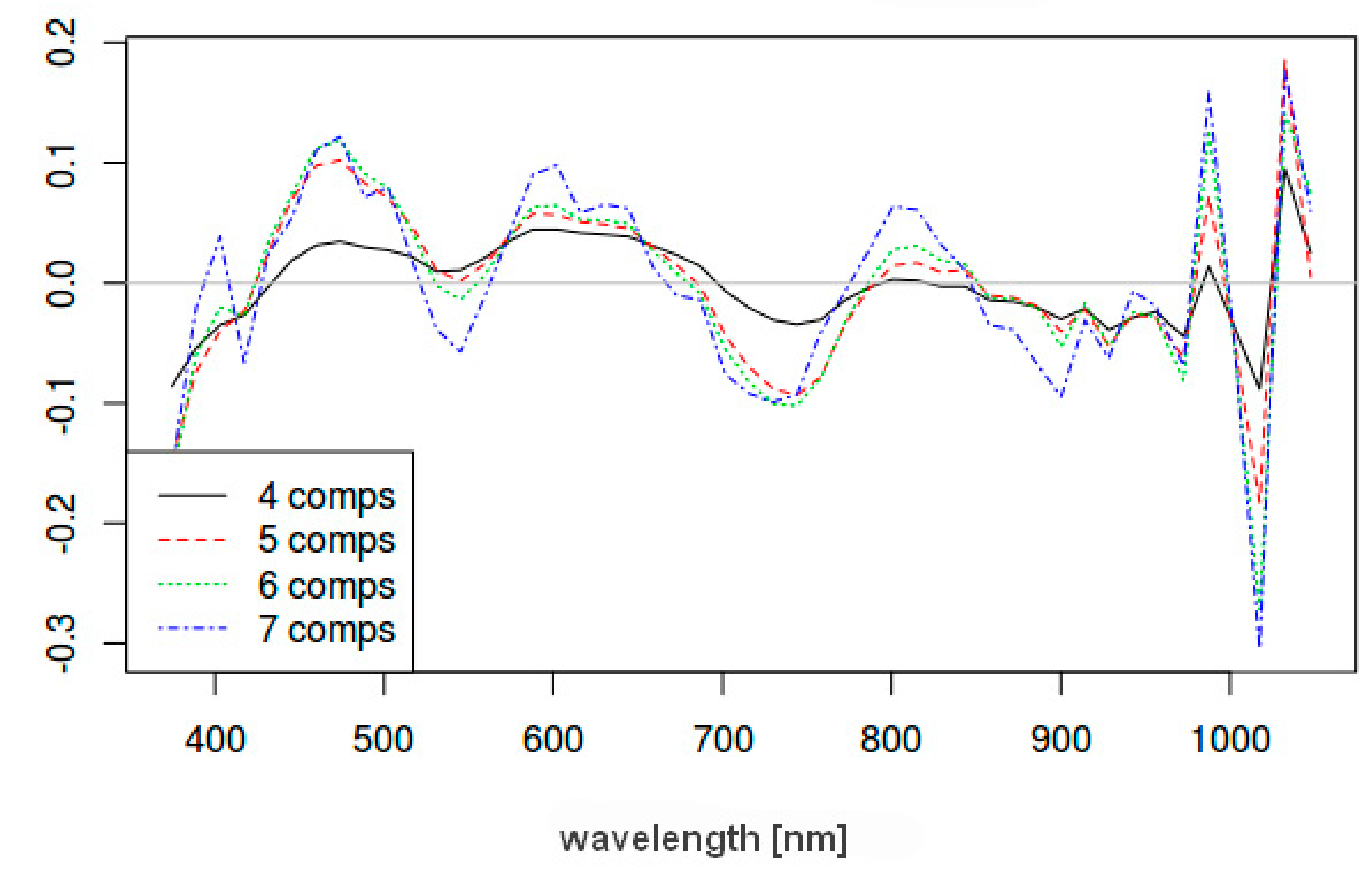
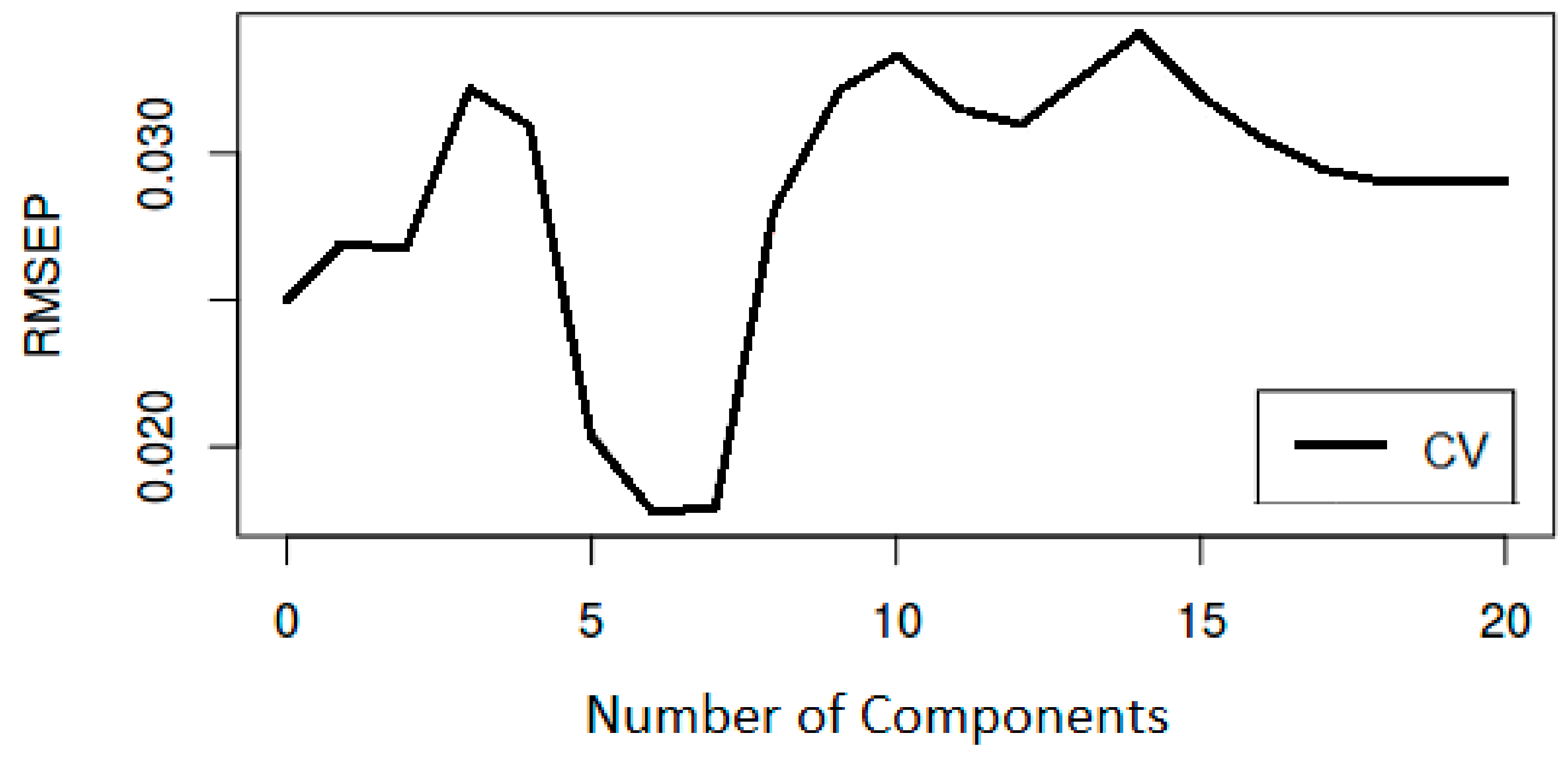
Regression vectors in Figure 7 show that the use of seven components contributes to the prediction, but this contribution is not significant and, according to cross-validation (Figure 8), there is a slight deterioration in the prediction ability. Although the use of seven components would not be wrong, only six were used to avoid over-fitting the model and, as a result, increasing the noise.

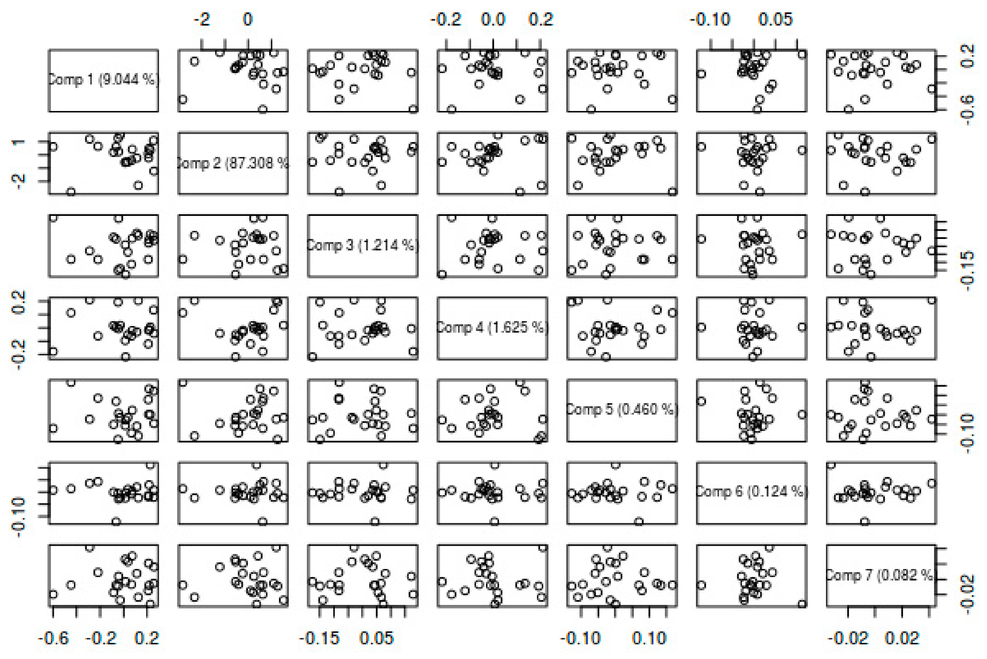
The decision to use six components is also supported by a score graph (Figure 8), which shows the variance of the data that make up the main components [46]. It is possible to read the variance of data between individual components from this graph. The most important component forming the model itself was the second component, explaining 87% of the problem relevant variance in the data. This is a rather surprising result because for most models built this way, the most important component is the first one. The sixth component is the most important for the second part of modeling and prediction. The values described by the sixth component are the values with the least variance and, except for two outliers, describe the data very well.

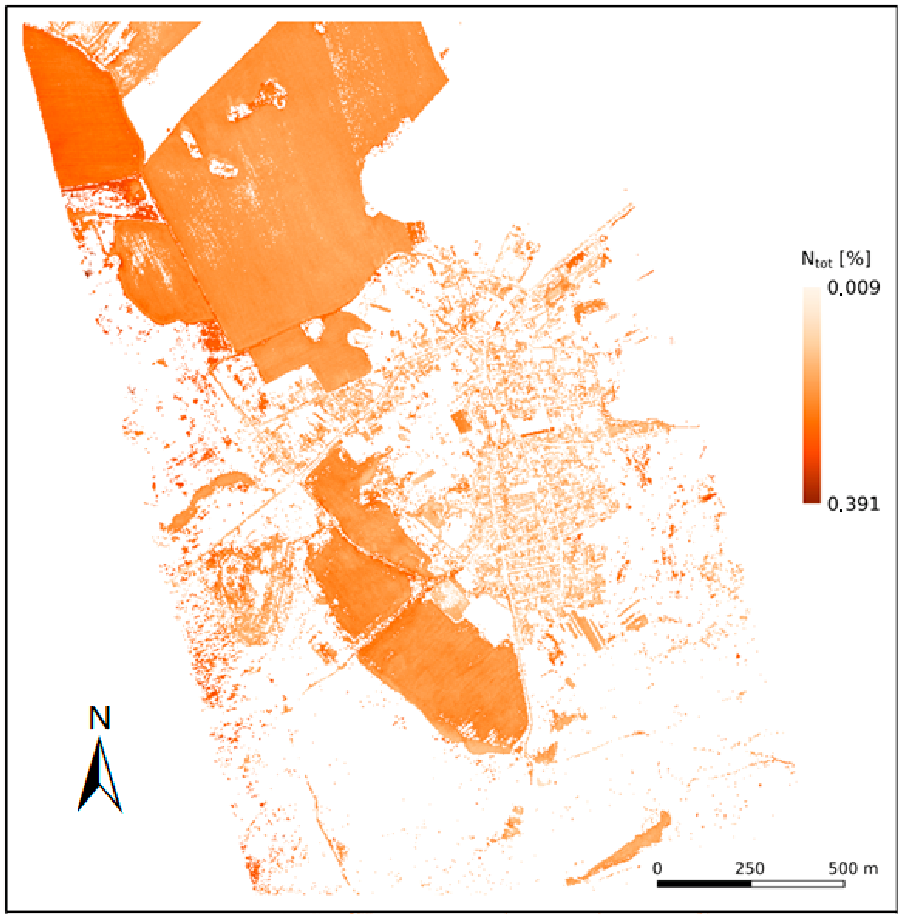
The main result of the prediction is a map that displays the spatial distribution of total soil nitrogen. The spatial component of the map output enables its immediate application in precision agriculture for spatially variable nitrogen management. The prediction results were refined by removing several negative values, which could be caused by low concentration or variability of the investigated element. Further refinement was made by removing those pixels that represent a surface (buildings and roads) for which the model was not built, and therefore, the resulting values for these surfaces are irrelevant.

It can be seen from

Table 6. Summary for measured and predicted values.

Basic Statistics	Measured Ntot (%)	Predicted Ntot (%)
Minimum	0.140	0.004
1st quartile	0.175	0.179
Median	0.190	0.194
Mean	0.189	0.199
3rd quartile	0.200	0.216
Maximum	0.245	0.391

that the predicted values were slightly higher than the values obtained by pedological measurements. This is due to the overall higher reflectance values on the hyperspectral image than the values measured by the handheld spectrometer.

Figure 9 shows a map with the spatial distribution of nitrogen values. It is possible to see that higher N concentrations were observed in the northwest area.

4. Discussion

The determination of total nitrogen in the soil is a very complex matter and involves several processes. Ideally, it is necessary to include all nitrogen cycles that can help to understand the evolution of nitrogen. However, these models will always be subject to a certain degree of error. Pedologists deal with assessing nitrogen mainly due to better management of nitrogen fertilizers. It is in the general interest to ensure high yields with minimal soil degradation [8].

Soil properties are most often determined in the laboratory. Unfortunately, classical laboratory methods are often time consuming, expensive, and destructive. Therefore, new methods are being developed to eliminate these disadvantages [6]. One of these new methods is laboratory spectroscopy. Another option is to employ remote sensing, which is probably the least expensive path and non-destructive to the soil. Aerial and satellite multispectral and hyperspectral images can map a relatively large area in a short time. However, when determining soil properties using this method, it is necessary to eliminate the influence of the atmosphere to achieve pure reflectance [13]. For example, aerial photography with a hyperspectral camera has been used in the past to detect nitrogen [47]. Of the satellite systems, the Hyperion hyperspectral system [48] or the Landsat 5 and 7 multispectral systems [9,49] are widely used.

The wavelengths suitable for examining soil nitrogen content vary considerably among published work. Dalal and Henry [22] determined the most suitable range of wavelengths to be 1100 to 2500 nm (more specifically 1702, 1870, and 2052 nm). On the other hand, Sterberg et al. [50] considered 1100, 1600, 1700, 1800, 2000, and 2200 nm to be the most appropriate wavelengths. Shi et al. [51] compared their results with previous works, which they incorporated into their work, and the output was a series of wavebands 1450, 1850, 2250, 2330, and 2400 nm. In this work, it is pointed out that the determination of suitable wavelengths depends mainly on the overall processing and the method used. The latter bands are especially suitable for nitrogen (but they can also be used for other soil properties) and for the popular PLSR method. In general, water absorption bands from 1300 to 3000 nm are the most suitable and most widely used for determining the soil nitrogen content [51,52]. The area is associated with water content, which changes the total carbon content in the soil. This suggests that the soil nitrogen content can be indirectly related to carbon content through these wavelengths [53]. Chang et al. [7] also pointed to a high correlation between the amount of these two elements in the soil.

Several studies have further compared the vis-NIR and MIR portions of the spectrum. MIR performed better in most of these studies [52,54,55]. The PLSR method or its variations (e.g., CARS-PLSR) were mostly used when working with MIR. Wavelengths suitable for measuring nitrogen in MIR were determined to be between 1676 and 1672, 1260 and 1036 cm⁻¹ [52].

In the present work, the PLSR method was used to develop a model for the prediction of total soil nitrogen for selected test locations. Unfortunately, the resulting parameters and prediction capabilities were not as high as results published in some previous studies reviewed by authors that have shown that this method can achieve accuracy higher than an R² of 0.8 [9,43]. The determining factor for the PLSR model presented in this paper reached an R² of 0.44, indicating that after cross-validation, the model describes data from which it was created with 44% confidence. Areas for improvement are listed below.

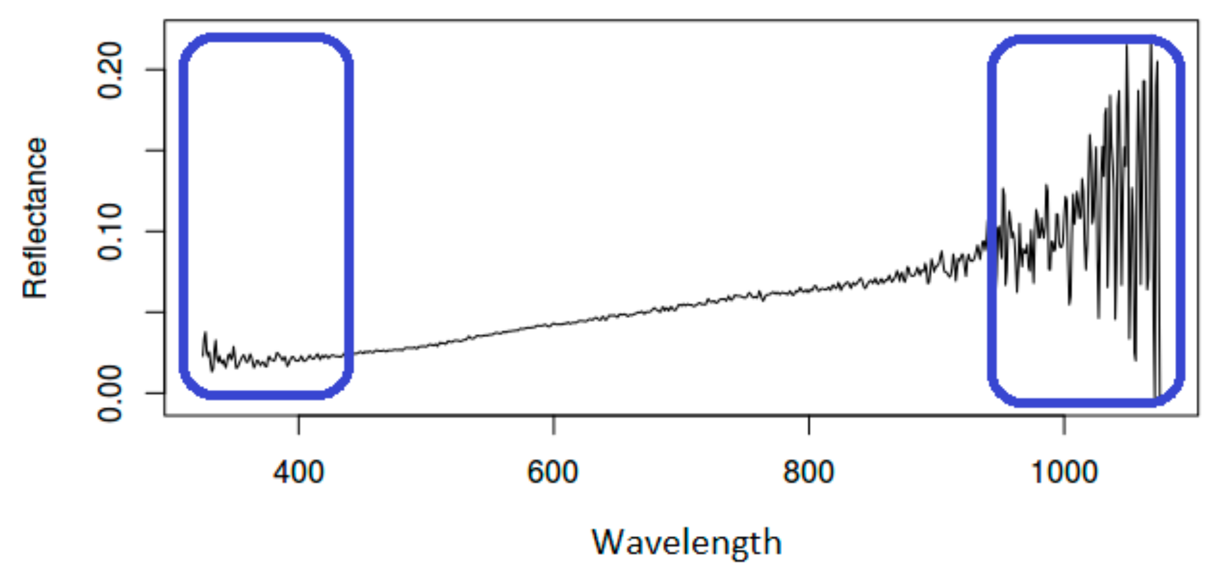
The primary disadvantage, when developing the PLSR model, concerns the spectral range of the handheld spectrometer used. The FieldSpec HandHeld2 spectrometer measures wavelengths in the range of 325–1075 nm with an excessive noise affecting the signal with a wavelength of less than 450 nm and greater than 950 nm. According to Vohland et al. [52], the critical wavelengths required to build a highly accurate model based on the spectral behavior of soil properties are in the NIR (near-infrared) and MIR (mid-infrared) bands starting at 750 nm. Using spectral information measured up to the infrared spectrum of the electromagnetic spectrum, Zornoza et al. [45] achieved results with an R² reaching up to 0.95 for total soil nitrogen content.

Another issue that possibly influenced the quality of the developed model was the different acquisition periods for the hyperspectral imaging (8 November 2016) and field data collection using a handheld spectrometer (7 October 2016), as the weather conditions for these two periods were different. Hyperspectral imaging was performed at lower temperatures, with possible ground frosts but minimal precipitation, while handheld spectrometer data were collected at higher temperatures with higher cloud coverage.

Finally, the low sample size was identified to affect the development of the model. The number of samples collected in our study (a total of 22 samples) was small and did not allow us to perform the second standard validation step. Unfortunately, with this low sample size, it was impossible to carry out a more rigorous statistical evaluation of the dataset and the selection of the most optimal samples. This small number of samples from only two different sites also caused the low variability of the total soil nitrogen, minimizing the ability to capture the key relationships between the soil property and the relevant spectral information. Studies that used hundreds of samples [47,56] achieved results with an R² higher than 0.8. Regarding the samples, some degree of uncertainty could also be due to laboratory measurements.

Based on the results, it was identified that close attention should be paid to datasets, as each can exhibit some degree of inaccuracy. In general, meteorological conditions, sample size, and the spectrometer parameters used for field data collection should be evaluated during the test preparation. The encountered problems could be significantly minimized by using a larger dataset sample and by implementing a public soil spectral library for the Czech region. Unfortunately, the only suitable soil spectral library, created at the Czech University of Life Sciences in Prague [57], was not publicly available. Therefore, field data collection was performed with the handheld spectrometer available to the authors.

5. Conclusions

The present work is a contribution to the wider use of remote sensing methods in precision agriculture. Nitrogen is a very complex component of soils that behaves unstably in time and space. Traditional methods for assessing the soil nitrogen content involve contact sampling and subsequent laboratory analysis. They achieve accurate results but have several practical limitations. They are time consuming, contact and destructive methods that require large numbers of samples to capture the soil variability. With frequent and repeated sampling, the land and cultivated plants are also degraded. The use of remote sensing data in the extended spectrum minimizes the disadvantages of traditional methods. Hyperspectral data are more suitable for determining the nitrogen supply than multispectral, and are often used in conjunction with statistical predictive modeling. According to the reviewed literature, the best models are created by employing the PLSR method, the applicability of which was subsequently tested in our work and confirmed this fact.

In our study, PLSR was applied to predict new values for total soil nitrogen based on data measured by a handheld spectrometer and laboratory-determined total soil nitrogen content. The developed model was then applied to the hyperspectral image to determine the predicted total nitrogen content of the soil. The application of PLSR was evaluated as a useful method for predicting soil properties in hyperspectral images. In our case, unfortunately, the method was not applicable for some soil properties and even the best model came out only with a medium predictive power (R² of 0.44). The results of the study showed the key role of input data quality in predictive modeling. The influence of atmospheric conditions in the collection of individual datasets and the necessity of using spectrometers covering the entire width of the spectrum in which soil nitrogen can be identified are significant.

References

1. Blum, W.E.H. Soil Resources—The Basis of Human Society and the Environment. Ressource Boden—Grundlage für Mensch und Umwelt. Die Bodenkultur 2006, 57, 197–202. [Google Scholar]
2. Skjemstad, J.O.; Clarke, P.; Golchin, A.; Oades, J.M. Characterization of soil organic matter by solid-state 13C NMR spectroscopy. In Driven by Nature: Plant Litter Quality and Decomposition; CAB International: Wellington, UK, 1997; pp. 253–271. [Google Scholar]
3. Hillel, D. Environmental Soil Physics; Academic Press Ltd.: London, UK, 1998. [Google Scholar]
4. Mattson, W.J. Herbivory in Relation to Plant Nitrogen Content. Annu. Rev. Ecol. Syst. 1980, 11, 119–161. [Google Scholar] [CrossRef]
5. Cassman, K.G.; Dobermann, A.; Walters, D.T. Agroecosystems, Nitrogen-use Efficiency, and Nitrogen Management. AMBIO J. Hum. Environ. 2002, 31, 132–140. [Google Scholar] [CrossRef] [PubMed]
6. Chang, C.-W.; Laird, D.A.; Mausbach, M.J.; Hurburgh, C.R. Near-Infrared Reflectance Spectroscopy-Principal Components Regression Analyses of Soil Properties. Soil Sci. Soc. Am. J. 2001, 65, 480–490. [Google Scholar] [CrossRef] [Green Version]
7. Chang, C.-W.; Laird, D.A. Near-Infrared Reflectance Spectroscopic Analysis of Soil Carbon and Nitrogen. Soil Sci. 2002, 167, 110–116. [Google Scholar] [CrossRef]
8. Li, S.; Ji, W.; Chen, S.; Peng, J.; Zhou, Y.; Shi, Z. Potential of VIS-NIR-SWIR Spectroscopy from the Chinese Soil Spectral Library for Assessment of Nitrogen Fertilization Rates in the Paddy-Rice Region, China. Remote Sens. 2015, 7, 7029–7043. [Google Scholar] [CrossRef] [Green Version]
9. Vågen, T.-G.; Shepherd, K.D.; Walsh, M.G. Sensing landscape level change in soil fertility following deforestation and conversion in the highlands of Madagascar using Vis-NIR spectroscopy. Geoderma 2006, 133, 281–294. [Google Scholar] [CrossRef]
10. Europen Space Agency (ESA). Sentinel Online. 2020. Available online: https://sentinel.esa.int/web/sentinel/missions/sentinel-2/instrument-payload/resolution-and-swath (accessed on 20 February 2021).
11. Liu, L.; Ji, M.; Buchroithner, M. Transfer Learning for Soil Spectroscopy Based on Convolutional Neural Networks and Its Application in Soil Clay Content Mapping Using Hyperspectral Imagery. Sensors 2018, 18, 3169. [Google Scholar] [CrossRef] [Green Version]
12. Sabins, F.F. Remote sensing for mineral exploration. Ore Geol. Rev. 1999, 14, 157–183. [Google Scholar] [CrossRef]
13. Gomez, C.; Rossel, R.A.V.; McBratney, A.B. Soil organic carbon prediction by hyperspectral remote sensing and field vis-NIR spectroscopy: An Australian case study. Geoderma 2008, 146, 403–411. [Google Scholar] [CrossRef]
14. Skauli, T.; Haavardsholm, T.; Kasen, I.; Opsahl, T.O.; Kavara, A.; Skaugen, A. Hyperspectral imaging technology and systems, exemplified by airborne real-time target detection. In Proceedings of the CLEO:2011—Laser Applications to Photonic Applications, Baltimore, MD, USA, 1–6 May 2011; pp. 1–3. [Google Scholar]
15. Caporaso, N.; Whitworth, M.B.; Fisk, I.D. Near-Infrared spectroscopy and hyperspectral imaging for non-destructive quality assessment of cereal grains. Appl. Spectrosc. Rev. 2018, 53, 667–687. [Google Scholar] [CrossRef] [Green Version]
16. Miller, C.E. Chemical principles of near-infrared technology. In Near-Infrared Technology in the Agricultural and Food Industries; Williams, P., Norris, K., Eds.; The American Association of Cereal Chemists Inc.: St. Paul, MN, USA, 2001; pp. 19–37. [Google Scholar]
17. Mortimore, J.L.; Marshall, L.-J.R.; Almond, M.J.; Hollins, P.; Matthews, W. Analysis of red and yellow ochre samples from Clearwell Caves and Çatalhöyük by vibrational spectroscopy and other techniques. Spectrochim. Acta Mol. Biomol. Spectrosc. 2004, 60, 1179–1188. [Google Scholar] [CrossRef]
18. Clark, R.N. Spectroscopy of Rocks and Minerals and Principles of Spectroscopy. In Remote Sensing for the Earth Sciences; Rencz, A.N., Ed.; John Wiley and Sons: Chichester, UK, 1999; pp. 3–58. [Google Scholar]
19. Viscarra Rossel, R.A.; McGlynn, R.N.; McBratney, A.B. Determing the composition of mineral-organic mixes using UV-vis-NIR diffuse reflectance spectroscopy. Geoderma 2006, 137, 70–82. [Google Scholar] [CrossRef]
20. Hunt, G.R.; Salisbury, J.W. Visible and Near-Infrared Spectra of Minerals and Rocks. I. Silicate minerals. Mod. Geol. 1970, 1, 283–300. [Google Scholar]
21. Ben-Dor, E.; Irons, J.R.; Epema, G.F. Soil Reflectance. In Remote Sensing for the Earth Sciences: Manual of Remote Sensing, 3rd ed.; Wiley: New York, NY, USA, 1999; Volume 3, pp. 111–188. [Google Scholar]
22. Dalal, R.C.; Henry, R.J. Simultaneous Determination of Moisture, Organic Carbon, and Total Nitrogen by Near Infrared Reflectance Spectrophotometry. Soil Sci. Soc. Am. J. 1986, 50, 120–123. [Google Scholar] [CrossRef]
23. Krishnan, P.; Alexander, J.D.; Butler, B.J.; Hummel, J.W. Reflectance Technique for Predicting Soil Organic Matter. Soil Sci. Soc. Am. J. 1980, 44, 1282–1285. [Google Scholar] [CrossRef]
24. Martin, P.D.; Malley, D.F.; Manning, G.; Fuller, L. Determination of soil organic carbon and nitrogen at the field level using near-infrared spectroscopy. Can. J. Soil Sci. 2002, 82, 413–422. [Google Scholar] [CrossRef]
25. Stenberg, B. Effects of Soil Sample Pretreatments and Standardized Rewetting as Interacted with Sand Classes on Vis-NIR Predictions of Clay and Soil Organic Carbon. Geoderma 2010, 158, 15–22. [Google Scholar] [CrossRef] [Green Version]
26. Viscarra Rossel, R.A.; Behrens, T. Using Data Mining to Model and Interpret Soil Diffuse Reflectance Spectra. Geoderma 2010, 158, 46–54. [Google Scholar] [CrossRef]
27. Martens, H.; Naes, T. Multivariate Calibration; John Wiley and Sons: Chichester, UK, 1989. [Google Scholar]
28. Viscarra Rossel, R.A.; Lark, R.M. Improved Analysis and Modelling of Soil Diffuse Reflectance Spectra Using Wavelets. Eur. J. Soil Sci. 2009, 60, 453–464. [Google Scholar] [CrossRef]
29. Viscarra Rossel, R.A. Robust Modelling of Soil Diffuse Reflectance Spectra by Bagging-Partial Least Squares Regression. J. Near Infrared Spectrosc. 2007, 15, 39–47. [Google Scholar] [CrossRef]
30. Mouazen, A.M.; Kuang, B.; De Baerdemaeker, J.; Ramon, H. Comparison between Principal Component, Partial Least Squares and Artificial Neural Network Analyses for Accuracy of Measurement of Selected Soil Properties with Visible and Near Infrared Spectroscopy. Geoderma 2010, 158, 23–31. [Google Scholar] [CrossRef]
31. The Food and Agriculture Organization. World Reference Base for Soil Resources 2014 (Update 2015); Food and Agriculture Organization of the United Nations: Rome, Italy, 2015. [Google Scholar]
32. Zbíral, J.; Honsa, I. Analyses of Soil I. Methodology; Central Institute for Supervising and Testing in Agriculture: Brno, Czech Republic, 2010; p. 197. (In Czech) [Google Scholar]
33. Malvern Panalytical. ASD HandHeld 2: Hand-held VNIR Spectroradiometer. Malvern Panalytical. 2018. Available online: https://www.malvernpanalytical.com/en/products/product-range/asd-range/fieldspec-range/handheld-2-hand-held-vnir-spectroradiometer (accessed on 23 July 2018).
34. Hanuš, J.; Fabiánek, T.; Kaplan, V.; Homolová, L. Flying laboratory of imaging systems (FLIS) at CzechGlobe. In Proceedings of the 14th International Multidisciplinary Scientific GeoConference SGEM 2014, Albena, Bulgaria, 17–26 June 2014; pp. 177–182. [Google Scholar]
35. Wold, S.; Sjöström, M.; Eriksson, L. PLS-Regression: A Basic Tool of Chemometrics. Chemom. Intell. Lab. Syst. 2001, 58, 109–130. [Google Scholar] [CrossRef]
36. Feilhauer, H.; Asner, G.P.; Martin, R.E.; Schmidtlein, S. Brightness-normalized Partial Least Squares Regression for hyperspectral data. J. Quant. Spectrosc. Radiat. Transf. 2010, 111, 1947–1957. [Google Scholar] [CrossRef]
37. Hbirkou, C.; Pätzold, S.; Mahlein, A.-K.; Welp, G. Airborne hyperspectral imaging of spatial soil organic carbon heterogeneity at the field-scale. Geoderma 2012, 175–176, 21–28. [Google Scholar] [CrossRef]
38. Roelofsen, H.D.; van Bodegom, P.M.; Kooistra, L.; van Amerongen, J.J.; Witte, J.-P.M. An evaluation of remote sensing derived soil pH and average spring groundwater table for ecological assessments. Int. J. Appl. Earth Obs. Geoinf. 2015, 43, 149–159. [Google Scholar] [CrossRef]
39. Nawi, N.M.; Chen, G.; Jensen, T. Visible and Shortwave Near Infrared Spectroscopy to Predict Sugarcane Quality from Clear and Raw Juice Samples. In Proceedings of the 3rd Malaysian Postgraduate Conference (MPC2013), Mandurah, WA, Australia, 1 January 2013; pp. 167–174. [Google Scholar]
40. Grant, L. Using Satellite Imagery and Novel Low Altitude Aerial Imagery to Classify Coastal Wetland Vegetation for Change Detection at Whatipu Scientific Reserve, Auckland, NZ. Master’s Thesis, Auckland University of Technology, Auckland, New Zealand, 2015. [Google Scholar]
41. Stevens, A.; Ramirez-Lopez, L. Package ‘Prospectr’—Miscellaneous Functions for Processing and Sample Selection of vis-NIR Diffuse Reflectance Data. 2013. Available online: https://github.com/antoinestevens/prospectr (accessed on 8 October 2018).
42. Melvik, B.H.; Wahrens, R. Introduction to the PLS Package. 2016. Available online: https://cran.r-project.org/web/packages/pls/vignettes/pls-manual.pdf (accessed on 24 July 2018).
43. Daughtry, C.; Hunt, E.R.; Walthallm, C.; Kramer, E.J. Assessing the Spatial Distribution of Plant Litter. Available online: https://www.researchgate.net/publication/265038260_ASSESSING_THE_SPATIAL_DISTRIBUTION_OF_PLAN (accessed on 18 September 2020).
44. Haboudane, D.; Millera, J.R.; Pattey, E.; Zarco-tejada, P.J.; Strachane, I.B. Hyperspectral vegetation indices and novel algorithms for predicting green LAI of crop canopies: Modeling and validation in the context of precision agriculture. Remote Sens. Environ. 2004, 90, 337–352. [Google Scholar] [CrossRef]
45. Gerighausen, H.; Menz, G.; Kaufmann, H. Spatially Explicit Estimation of Clay and Organic Carbon Content in Agricultural Soils Using Multi-Annual Imaging Spectroscopy Data. Appl. Environ. Soil Sci. 2012, 2012, 868090. [Google Scholar] [CrossRef]
46. Dunn, K.; Interpreting the Scores in PLS. Process Improvement Using Data. Available online: https://learnche.org/pid/latent-variable-modelling/projection-to-latent-structures/interpreting-pls-scores-and-loadings (accessed on 22 October 2020).
47. Hively, W.D.; McCarty, G.W.; Reeves, J.B.; Lang, M.W.; Oesterling, R.A.; Delwiche, S.R. Use of Airborne Hyperspectral Imagery to Map Soil Properties in Tilled Agricultural Fields. Appl. Environ. Soil Sci. 2011, 2011, 358193. [Google Scholar] [CrossRef] [Green Version]
48. Lu, P.; Wang, L.; Niu, Z.; Li, L.; Zhang, W. Prediction of soil properties using laboratory VIS–NIR spectroscopy and Hyperion imagery. J. Geochem. Explor. 2013, 132, 26–33. [Google Scholar] [CrossRef]
49. Rivero, R.; Grunwald, S.; Binford, M.; Osborne, T. Integrating spectral indices into prediction models of soil phosphorus in a subtropical wetland. Remote Sens. Environ. 2009, 113, 2389–2402. [Google Scholar] [CrossRef]
50. Stenberg, B.; Viscarra Rossel, R.A.; Mouazen, A.M.; Wetterlind, J. Visible and Near Infrared Spectroscopy in Soil Science. Available online: http://0-linkinghub-elsevier-com.brum.beds.ac.uk/retrieve/pii/S0065211310070057 (accessed on 4 October 2016).
51. Shi, T.; Cui, L.; Wang, J.; Fei, T.; Chen, Y.; Wu, G. Comparison of multivariate methods for estimating soil total nitrogen with visible/near-infrared spectroscopy. Plant Soil 2013, 366, 363–375. [Google Scholar] [CrossRef]
52. Vohland, M.; Ludwig, M.; Thiele-Bruhn, S.; Ludwig, B. Determination of soil properties with visible to near- and mid-infrared spectroscopy: Effects of spectral variable selection. Geoderma 2014, 223–225, 88–96. [Google Scholar] [CrossRef]
53. Morra, M.J.; Hall, M.H.; Freeborn, L.L. Carbon and Nitrogen Analysis of Soil Fractions Using Near-Infrared Reflectance Spectroscopy. Soil Sci. Soc. Am. J. 1991, 55, 288–291. [Google Scholar] [CrossRef]
54. Iii, J.B.R.; Follett, R.F.; Mccarty, G.W.; Kimble, J.M. Can Near or Mid-Infrared Diffuse Reflectance Spectroscopy Be Used to Determine Soil Carbon Pools? Commun. Soil Sci. Plant Anal. 2006, 37, 2307–2325. [Google Scholar] [CrossRef]
55. Bellon-Maurel, V.; Fernandez-Ahumada, E.; Palagos, B.; Roger, J.-M.; McBratney, A. Critical review of chemometric indicators commonly used for assessing the quality of the prediction of soil attributes by NIR spectroscopy. TrAC Trends Anal. Chem. 2010, 29, 1073–1081. [Google Scholar] [CrossRef]
56. Zornoza, R.; Guerrero, C.; Mataix-Solera, J.; Scow, K.; Arcenegui, V.; Mataix-Beneyto, J. Near infrared spectroscopy for determination of various physical, chemical and biochemical properties in Mediterranean soils. Soil Biol. Biochem. 2008, 40, 1923–1930. [Google Scholar] [CrossRef] [Green Version]
57. Brodsky, L.; Klement, A.; Penizek, V.; Kodešová, R.; Borůvka, L. Building soil spectral library of the Czech soils for quantitative digital soil mapping. Soil Water Res. 2011, 6, 165–172. [Google Scholar] [CrossRef] [Green Version]
Figure 1. Location of Rudice in the Czech Republic (imagery: Sentinel-2).
Ijgi 10 00355 g001
Figure 2. Schematic flowchart for predicting soil total nitrogen using PLSR method.
Ijgi 10 00355 g002
Figure 3. Sample reflectance of the soil sample measured with FieldSpec HandHeld2 Spectrometer.
Ijgi 10 00355 g003
Figure 4. False color FLIS hyperspectral image (band 9 as red, band 40 as green, and band 67 as blue).
Ijgi 10 00355 g004
Figure 5. Validation of model performance based on number of used latent components.
Ijgi 10 00355 g005
Figure 6. Model prediction of N-absorbance using six components.
Ijgi 10 00355 g006
Figure 7. Regression coefficients for four to seven components. The y-axis shows the values of the regression coefficient.
Ijgi 10 00355 g007
Figure 8. Score plot of the best model for first seven components.
Ijgi 10 00355 g008
Figure 9. Sample of total soil nitrogen raster output, which contains predicted values for total soil nitrogen (Ntot) from 8 November 2016.
Ijgi 10 00355 g009