1. Introduction
Social media has become a mainstream channel of communication where users share and exchange information. In the last decade, social media platforms have grown in popularity and are readily available on mobile devices to connect users to streams of information. Among social media sites, Twitter has more than 320 million users generating 500 million tweets per day [
1]. In 2019, the number of monthly active US Twitter users reached 68 million [
2]. Twitter comments are restricted to 280 characters and are mostly publicly available. Twitter users can participate in social media activities such as sharing their messages (tweets) or reposting previously published messages (retweets) [
3].
Twitter Application Programming Interfaces (APIs) are, collectively, a tool for collecting user data. Twitter API data is now the main social media data source for researchers and policymakers [
3]. In the last decade, there has been a marked increase in using Twitter data for research, and we expect to see more Twitter-related studies in the following years [
3]. A large number of studies have utilized Twitter data for diverse research interests, such as analyzing the content of tweets related to health issues, such as happiness, diet, and physical activity [
4], health disinformation [
5], mental health [
6], food [
7], and LGBT health [
8]; understanding Twitter discussions during natural disasters, such as Hurricane Sandy [
9]; and mining public opinion during different events, such as the 2016 U.S. elections [
10] and the #metoo movement representing sexual harassment experiences [
11].
Current literature has utilized quantitative or qualitative methods to analyze Twitter data, such as utilizing machine learning classification methods for sentiment analysis [
4], identifying self-expressions of mental illness diagnoses [
6], and classifying sexual harassment experiences [
11]; text mining techniques for disclosing the semantic of tweets regarding disinformation [
5] and LGBT health [
8]; and qualitative coding for examining information sharing strategies of social bot information [
12].
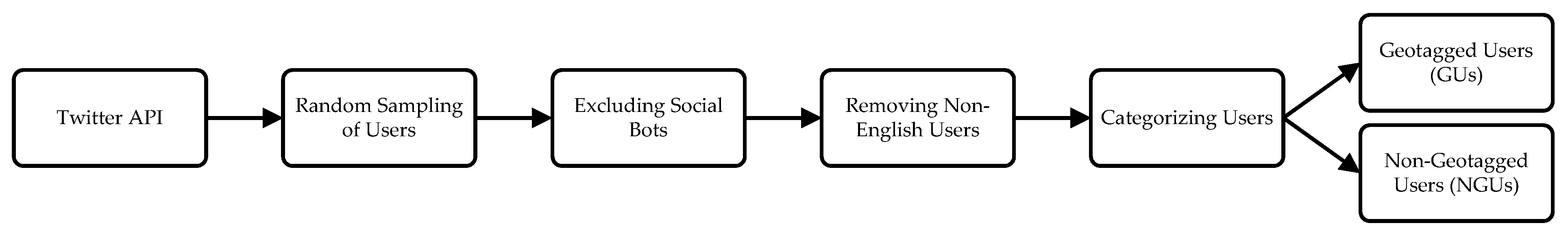
Twitter users can use three methods to share their location [
13]. In the first method, users share their location on their Twitter profile. In the second method, users mention their location in tweets. In the last one, users share their longitude and latitude information through a process called geotagging. The first and the second methods have limitations. They offer broad areas (e.g., city and state) and do not show the movement of users. However, the third method overcomes the limitations and shows precise real-time locations of users. These features have made the third method an attractive accurate format for research [
13]. The focus of this research is on geotagging users who share at least one geotagged tweet.
It has been estimated that 4 million geotagged tweets are posted every day [
13]. The location data is valuable for researchers to identify spatial patterns and link Twitter data to external datasets, such as the Behavioral Risk Factor Surveillance System (BRFSS) [
4] to provide better perspectives on different issues. The location data can reveal different information, such as where users live and work [
13]. Therefore, studying geotagged Twitter data can provide more research dimensions, such as comparing the content of tweets regarding different locations.
It has been shown that spatial analysis of Twitter data has attracted researchers [
3]. A wide range of studies has been developed based on geotagged Twitter data, such as exploring the diversity of human mobility patterns among individuals and within/between cities [
14] and during the COVID-19 pandemic [
15,
16]; identifying spatiotemporal patterns of tweets during floods and hurricanes [
17,
18]; analyzing tweets containing discussions on climate change [
19]; recognizing health patterns regarding obesity [
20,
21,
22,
23], diabetes [
20], happiness [
4], diets and foods [
4,
24,
25], physical activities [
4], drug-related health problems [
26], and Zika virus [
27,
28]; and studying geotagging behavior, such as the motivation behind geotagging [
29] and patterns of geotagging [
30].
The above studies assumed that geotagged users (GUs) can represent non-geotagged users (NGUs). Their reason is that most scientists optimize their data collection by obtaining data samples [
31]. Compared to the mostly small-scale data samples in different domains, such as social science [
32], collecting geotagged tweets offers large samples. While geotagged Twitter data offer a great opportunity for researchers to identify and study spatial patterns, less than 1% of Tweets are geotagged [
33,
34]. This small proportion of tweets imposes a negative impact on obtaining tweets containing specific terms [
35]. There is a fundamental question whether geotagged tweets and users can represent non-geotagged ones [
13,
36]. In other words, do geotagged users constitute a random sample of the Twitter population or are they significantly different? This question has encouraged researchers to compare Twitter geotagged and non-geotagged users and tweets [
13,
36]. Comparing geotagged and non-geotagged tweets and users reveals whether geotagged tweets and users are representative of non-geotagged tweets and users. Two studies compared geotagged and non-geotagged users. The first study showed that there is a significant difference between the users who share and the users who do not share their location based on demographic characteristics, such as age and gender [
13]. The second study found that there is a significant difference among geotagged and non-geotagged users based on types of device, country, and language. In addition, the users who share their location on their profile were found to be more likely to use a geotagging service and connect to users with similar geotagging behavior than the users who do not share their location [
36].
While the two studies have provided valuable perspectives, they did not investigate profile information and the content of tweets of geotagged and non-geotagged users. Considering this limitation, we expanded the previous work by comparing geotagged users (GUs) and non-geotagged users (NGUs) based on profile information and the content of tweets. Specifically, this study aims to investigate Twitter activities and information sharing patterns of GUs and NGUs. To do this, this paper has collected and analyzed data of more than 88,000 Twitter users to address the following research questions.
RQ1: Is there a significant difference between geotagged and non-geotagged users regarding Twitter profile information?
RQ2: Is there a significant difference between geotagged and non-geotagged users based on the content of tweets?
RQ3: To what extent can the identified features in RQ1 and RQ2 distinguish between geotagged and non-geotagged users?
While addressing RQ3 discloses the prediction power of the features to distinguish between GUs and NGUs, investigating RQ1 and RQ2 reveals whether geotagged users can represent non-geotagged users based on the content features of Twitter profiles and tweets. If there are no discernible differences between GUs and NGUs regarding the features in RQ1 and RQ2, we can consider GUs as representative of NGUs. Otherwise, there is a need to consider methods for ameliorating or controlling.
2. Materials and Methods
This section provides details on data collection and pre-processing, feature extraction, statistical comparison, and prediction analysis.
2.1. Data
While relevant studies did not filter out bots [
13,
36], this study addresses this limitation. To remove bots and users who post tweets written in non-English languages, we utilized Botometer (
https://botometer.osome.iu.edu/, accessed on 30 May 2021), which analyzes Twitter profile features (e.g., number of tweets) with machine learning. This tool assigns a score from 0 (human) to 5 (bot) to each of Twitter accounts and discloses the language of the users [
37]. We removed the accounts that were assigned a Botometer’s score between 4 and 5, which is the red zone defined by Botometer, and posted tweets written in non-English languages. This process provided 88,976 Twitter users. Due to the API limitation, we were able to collect up to 3200 tweets per user.
One approach to infer the location is identifying geotagged tweets [
34]. This approach assumes that geotagged tweets can help to infer location information. This assumption indicates that, if a user posts a tweet that does not have geotagging information, other geotagged tweets of the user can assist in inferring the location of users. Based on this assumption and similar to [
13], we categorized the users into two groups. The first group (GU) included users who shared at least one geotagged tweet containing latitude and longitude coordinates, and the second group (NGU) included users who did not post any geotagged tweets. The final dataset was a list of users with a binary class, GU or NGU.
As we did not define a timeframe and collected tweets without any queries, our data is a representative sample, and we can apply statistical tests to investigate the research questions. Our dataset includes tweets posted in 2020 and before. For example, if one user created an account in 2015 and we collected her/his tweets in 2020, those tweets were posted between 2015 and 2020. In addition, more than 97.82% of accounts had been active for more than three years.
While Twitter stopped adding a precise geotag to tweets in 2019 (
https://twitter.com/TwitterSupport/status/1141039841993355264?s=20, accessed on 30 May 2021), we were able to tag the precise location (latitude and longitude) of photographs and add our location to tweets via the service’s integration with mapping services [
38]. This means that, if a user takes a photo, tags the precise location in the photo using camera applications in her/his phone device, and shares the photo in a tweet, the Twitter API can find the precise location.
2.2. Feature Extraction
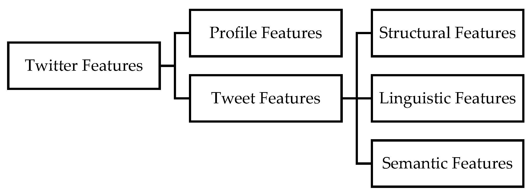
This research compared GUs and NGUs based on two types of features, including the profile features of Twitter users and the content features of tweets (
Figure 2), to address RQ1–RQ3. The tweet features had three sub-features, including structural, linguistic, and semantic features.
To address RQ1, we obtained six structured features from Twitter profiles, including the number of followers, followings, tweets + retweets (RTs), words in bio, favorites, and the age of the account. The null hypothesis of RQ1 is that there is not a significant difference between GUS and NGUS regarding Twitter profile information.
To address RQ2, we obtained both structured and unstructured features from the content of tweets. The null hypothesis of RQ2 is that there is not a significant difference between GUS and NGUS based on structured and unstructured features of tweets. The structured features represent the structural features of tweets, such as the average number of hashtags per tweet. Those features are based on the frequency of tweets, RTs, URLs, hashtags (#), and at signs (@). These features illustrate how users shape and share their tweets.
Table 1 shows definitions of Twitter terminology.
The unstructured features illustrate the content features of tweets. We analyzed the unstructured features based on linguistic and semantic features. We processed unstructured features in the content of tweets using two strategies.
The first strategy obtained linguistic features using linguistic inquiry and word count (LIWC). This tool processes a document and counts the percentage of words that reflect different emotions, thinking styles, social concerns, and parts of speech within a group of built-in dictionaries [
39]. This program was developed in the Java programming language with almost 6400 words, word stems, and selected emoticons [
39]. Each dictionary word was mapped to one or multiple word categories using LIWC. For example, the word “cried” can be mapped to five categories: Sadness, Negative Emotion, Overall Affect, Verb, and Past Focus. LIWC has been used for different applications, such as opinion mining [
40] and spam detection [
41].
LIWC has also been applied in research utilizing geotagged tweets for difference purposes. One study investigated whether Twitter-derived linguistic variables are predictive of a county’s health statistics [
42]. This study predicted county-level health statistics of the top 100 most populous counties in the US using different features in the content of tweets, such as LIWC features. A similar study has used LIWC to predict county-wide obesity and diabetes [
23].
The second strategy to understand unstructured tweets was utilizing topic modeling to disclose the hidden semantic layer of tweets. Among topic models, we chose latent Dirichlet allocation (LDA) [
43], which has been considered an effective model [
44]. LDA has been utilized for different applications, such as analyzing medical documents to understand clinical notes [
45], exploring the content of research papers to identify trends and patterns [
46,
47,
48], and mining social media to understand online discussions [
49,
50,
51,
52]. LDA is a generative model that assumes that there is an exchange between words and documents in a corpus represented by bag-of-words using the occurrence of words within a document to represent a corpus. LDA assigns semantically related words to a cluster called a topic. For example, LDA allocates “data”, “number”, and “computer” to a topic that is interpreted as a theme related to information technology [
53].
In this paper, a document represents up to 3200 tweets from a single user. For
n documents,
m words, and
t topics, the outputs of LDA are two matrices. The first one is the probability of each word given a topic, or
P(Wi|Tk), and the second one is the probability of each topic given a document, or
P(Tk|Dj) [
54]:
| Topics | | Documents |
| & | |
| P(Wi|Tk) | | P(Tk|Dj) |
We defined the retrieved tweets from one user as one document and obtained
P(T|D) to find the probability of topics given a document. Then, we utilized the Java-based MALLET [
55] to apply LDA to the tweets. Using the Mallet, we removed stopwords (e.g., “the”) and obtained
P(T|D) for three sets of topics, including 10, 25, and 50 topics. To define the LDA hyperparameters, we followed the literature [
46,
56] and selected
at 0.01 and
based on
, where
T is the number of topics.
2.3. Statistical Comparison
We investigated 194 features, including six profile features and 10 structural, 93 linguistic, and 85 semantic features of tweets, obtained from Twitter profiles and the content of tweets. We developed statistical tests using the two-sample t-test developed in the R mosaic package [
57] to compare GUs and NGUs based on the mean of features. The level of significance level should be set based on sample size [
58] using
[
59], where N is the number of users (88,976). So, the passing
p-value would be 0.001. To minimize both false positives and false negatives, we adjusted
p-values by controlling the false discovery rate (FDR) [
60]. Regarding RQ1 and RQ2, our alternative hypothesis was that there was a significant difference between GUs and NGUs regarding the features.
2.4. Prediction Analysis
To address RQ3, we developed a quantitative evaluation based on the profile features and structured, linguistic, and semantic features of tweets. This experiment shows how accurate a classifier can distinguish between GUs and NGUs regarding the 194 features. We hypothesized empirically that the features could help to identify (predict) GUs and NGUs without obtaining location information. In this classification, a classifier assigns a binary class (GU or NGU) to each user. To develop the classifier, we followed the framework in
Figure 3.
In our classification formulation, there are
n documents
. Each document represents the tweets of each user. The classification task predicts whether
is GU or NGU utilizing a classifier (c) that assigns a label (l) to
:
The classifier uses a set of
n features,
F =
obtained from the profile and tweets of users [
61]. To determine the class of each user, we utilized Random Forest, which is a high-performance classification method [
62] developed in Weka (
https://www.cs.waikato.ac.nz/ml/weka/, accessed on 30 May 2021). We used three-fold cross-validation, in which the data are broken into three subsets, and the holdout method is repeated three times. Each time, one of the three subsets is used as the test set and the other two subsets are used as the training set. To evaluate the classifier, we used the following confusion matrix [
63]:
| | | Predicted |
| | | GU | NGU |
| Actual | GU | True Positive (TP) | False Positive (FP) |
| NGU | False Negative (FN) | True Negative (TN) |
We measured precision, recall, accuracy, F-measure, and area under the ROC curve (AUC) based on the following definitions:
ROC shows the tradeoff between FP and TP by plotting FP on the X-axis and TP on the Y-axis. We provided the features (independent variables) for prediction and used all features, not just those features that satisfied the significance test, to find whether a user is a GU or NGU (dependent variable).
3. Results
We obtained more than 173 million tweets with more than 823 million tokens. Our data contained 18,116 GUs with more than 40 million tweets and 70,860 NGUs with more than 132 million tweets (
Table 2). On average, we retrieved 1950.7 tweets per user. The proportion of GUs is much higher than the 1% estimation of geotagged tweets [
33,
34] because this research focuses on users rather than tweets.
Figure 4 shows the distribution of the number of retrieved tweets per user. In our dataset, 99.09%, 91.43%, 67.67%, 53.38%, and 39.55% of the users have at least 10, 100, 1000, 2000, and 3000 retrieved tweets, respectively. This result indicates that most users have a considerable number of tweets in our dataset.
Considering GUs, the number of geotagged tweets per user is between 1 and 3163 with median 15 and mean 83.95. Our analysis shows that 15%, 27.2%, 37.5%, 16.9%, and 3.4% of GUs posted one, 2–10, 11–100, 101–500, and more than 500 geotagged tweet(s), respectively. This illustrates that 85% of GUs posted more than one geotagged tweet.
To address RQ1, we compared the profile information for the two groups and found that there is a very significant difference (adjusted
p-value
≤ 0.001) between GUs and NGUs based on the mean of the number of followers, tweets + RTs, words in the bio, and the account age (
Table 3). While this analysis shows that NGUs have a larger number of followers and post a larger number of tweets and retweets than GUs, the number of words in the bio and the account’s age are larger for GUs than NGUs. These two groups have a similar number of followings and favorites.
For RQ2, we built our experiments on structural, linguistic, and semantic features. Considering the structural features of tweets, we standardized the features with the total number of tweets or retweets. Our comparison analysis showed that there was a significant difference (adjusted
p-value ≤ 0.001) between GUs and NGUs based on seven out of ten features (
Table 4). Out of the seven features, we found that the average weight of three features was higher for NGUs than GUs. For example, NGUs retweet more than GUs.
Considering the linguistic features of tweets, LIWC helped this study to obtain 93 linguistic features of retrieved tweets for each user. This tool provided the total number of words (WC) in the tweets of a user. To standardize WC, we divided WC by the total number of retrieved tweets and retweets. Our analysis showed that there was a significant difference between GUs and NGUs based on 78 features (
Table 5). For example, the average number of words per tweet and retweet was higher for NGUs, and GUs used more positive words than NGUs. This finding illustrates that GUs have different preferences than NGUs on choosing words (e.g., pronouns) and discussing issues (e.g., religious). The differences are reflected in clout (i.e., the authority of the author), authenticity (i.e., honest self-depiction), and tone (i.e., the emotional inclination of the author) [
64]. These four variables represent a summary of some other variables [
39]. For example, the clout category includes we, social words, I, negations (e.g., no, not), and swear words, illustrating social hierarchy [
65,
66]. For more information on each of the 93 features, refer to [
39].
Considering the semantic features of tweets, we compared GUs and NGUs based on three sets of topics, including 10, 25, and 50 (total 85 topics), generated by LDA. We used the statistical tests to compare GUs and NGUs based on the average weight of each topic given the tweets of a user. Each topic represented a theme, such as an election. This analysis showed the preference of topics for GUs and NGUs. Our comparison analysis showed that the difference between GUs and NGUs was significant (adjusted
p-value ≤ 0.001) in more than 60% of the topics (
Table 6). We also found that the difference between GUs and NGUs expanded by increasing the number of topics from 10 to 50.
For RQ3, we developed three models, including all features with a different number of topics. We applied Random Forest on each model. These classification models infer whether a user has at least one geotagged tweet.
Table 7 summarizes the performance metrics of the three models. Our binary classification experiments are based on the profile features (PR) and structured (ST), linguistic (LI), and semantic (SE) features of tweets. Our findings indicate that the features can show whether a user shares geotagged tweets with around 80% accuracy, and GUs and NGUs can be seen as two distinct groups (
Table 7).
The model with 25 topics offered the highest classification performance, including accuracy of 80.40%, F-measure of 0.742, and AUC of 0.778. Although we have thus far shown that there is a significant difference between GUs and NGUs regarding most PR, ST, LI, and SE features examined independently, the classification experiments illustrate that the combination of the features is different for GUs and NGUs. According to the
t-test, the improvement of Random Forest over ZeroR, which relies on the target and ignores all predictors, is statistically significant. We also compared the three sets of features in
Table 5 using the paired
t-test and found that there is a significant difference among the three sets. The classification showed acceptable accuracy (
Table 7) and precision (
Table 8), but the recall was low for the GU class. While the goal of this paper is not to predict GUs and NGUs, future study can incorporate other features to improve the recall.
4. Discussion
Twitter users can share their exact location when they post their tweets by using the geotagging feature. The location of users is a valuable data source and can be linked to external datasets (e.g., Census Bureau) to enrich social media data and provide a multiple-perspective analysis, such as exploring public opinion on a topic (e.g., election) across different locations. While the proportion of users who enable their geotagging is very low [
67], four million geotagged tweets are posted per day [
13]. Obtaining spatial data and developing spatial analysis on social media are interesting for not only researchers [
3] but also companies for different business purposes, such as developing targeted real-time social media advertisements to enhance services and products [
68].
In the literature, there is an assumption that users who geotag their tweets could represent all Twitter users [
33,
34]. Thus, they could not report any significant difference between geotagged and non-geotagged users. While there are few studies that compare these two groups, there is no research comparing GUs and NGUs based on the content of profile and tweets. This research addresses this limitation by comparing GUs and NGUs based on 194 variables (features) obtained from profiles and tweets of GUs and NGUs. This paper set out to address three research questions.
This study illustrates that there is a significant difference between GUs and NGUs based on 143 features (73% of the 194 features). Therefore, the assumption of no difference between the two groups is not accurate, and geotagged users may not represent non-geotagged users. Our data size indicates that we can be confident that our findings are not due to random chance.
This study indicates that information sharing and the behavior of GUs and NGUs are mostly different. For example, compared to NGUs, geotagged users have been on Twitter for a longer time and prefer to disclose more information about themselves using more words in their profile bio. However, NGUs have more followers and post a higher number of tweets and retweets. While NGUs like retweets, having URLs in their tweets and retweets, and mentioning other users in their posts, GUs prefer tweets (instead of retweets) and using more hashtags.
This paper also shows that GUs and NGUs use different linguistics patterns. For instance, NGUs use more words in their tweets and retweets and talk about work and money more than GUs. Geotagged users post tweets and prefer using pronouns such as “I” and positive words and share more information about home and leisure than NGUs. This is an important finding because, for example, if researchers only analyze geotagged users or tweets to understand public opinion regarding a candidate during an election, they might conclude Twitter users have a positive opinion with respect to that candidate. However, it might simply reflect the fact that GUs are willing to post positive tweets.
Our semantic analysis using topic modeling also shows that GUs and NGUs have different preferences in terms of topical themes, indicating that GUs and NGUs do not share similar interests in their Twitter posts. Suppose that GUs are more interested in topic x than topic y, but NGUs prefer topic y more than topic x; therefore, analyzing geotagged tweets can lead us to conclude that Twitter users are more interested in topic x than topic y. However, the reason behind this conclusion is that NGUs are excluded from the analysis. For example, we found that GUs shows more interest in talking about different foods than NGUs. In this case, diet experts might overestimate food consumption of Twitter users if they focus on geotagged users.
Previous studies have shown that there is a significant difference between GUs and NGUs based on demographics, types of device, country, language, profile location, and the geotagging preference of their friends. In brief, the findings of previous studies and our results indicate that the geotagged users are not representative of the Twitter population. To address this limitation, there is a need to utilize methods to not only use profile information but also infer the location of NGUs through utilizing profile information [
34], the user’s network of friends [
69], time zones [
34], the content of tweets [
70], URL links [
34], combination of different features such as profile information, the content of tweets, and place labelling in tweets [
71,
72].
This research concludes that GUs and NGUs have different preferences on topics of interest and creating and sharing social media posts. This study offers an empirical foundation to inform research on geotagged Twitter data, such as monitoring health issues and public opinion. The impact of our results will depend on the topic being studied. If researchers need to analyze geotagged users for a specific study, we suggest investigating whether there is a significant difference between GUs and NGUs on a data sample. Otherwise, their results would not be generalizable to the entire Twitter population. This suggestion helps to improve the generality power of Twitter studies investigating spatial factors by increasing the number of users whose location is identified. We also suggest researchers who are interested in linking Twitter data to external datasets to explore whether there is a significant correlation between Twitter data and external characteristics, such as socio-demographic factors, before further investigation [
73].
While this study examined important research questions, there are some limitations. First, we were not aware of demographic information about users (e.g., gender). Second, the focus of this study was limited to tweets written in English. Third, this research was limited to geotagged users on the Twitter population, not other types of users and the real-world population. Fourth, while we obtained a random sample of Twitter users, this study does not consider spatial and temporal factors. Fifth, we assumed GUs are the ones who share at least one geotagged tweet. However, we did not investigate whether there is a statistical difference between GUs with high and low number of geotagged tweets. Future work could address these limitations by utilizing methods to infer demographic information such as the gender of users (e.g., analyzing the name of users), analyzing non-English tweets, studying other types of location Twitter sharing strategies, such as place-tagging, investigating differences regarding different times and locations, exploring categories of GUs based on the number of geotagged tweets, and analyzing special and temporal factors such as spatiotemporal analysis of tweets [
74]. It would also be interesting to expand this study by comparing users based on their county (e.g., GUs vs. NGUs in Canada or France). It was found that most geotagged tweets are from non-Twitter platforms, such as Instagram [
36]. Therefore, comparing the geotagging behavior of users regarding different platform could be an interesting extension of this paper. In addition, while digging into the details of the detected differences is beyond the scope of this research, understanding the reasons behind the identified differences would be a fruitful future avenue of research.
To conclude, the contributions of this paper are five-fold. First, this is the first research that compares GUs and NGUs based on profile information and the content of tweets on Twitter. Second, this study shows GUs and NGUs mostly have different information sharing behavior. Third, GUs and NGUs have distinct linguistics choices and topics of interests. Fourth, this work offers new directions in studying location sharing behavior. Fifth, this paper proposes suggestions for controlling adverse effects of sampling geotagged users and tweets. The contributions of this paper can be used by studies utilizing geo-tagged Twitter data for studying the content of profile and tweets and their linguistics and semantic pattern.


 ,
, 


