
Remote Sensing Methods for the Biophysical Characterization of Protected Areas Globally: Challenges and Opportunities

 , , , , and
Abstract
:1. Introduction
2. Relevant Ecological Units and Descriptors
3. Global Characterization of Protected Areas
3.1. Global Input Variables and Data Sources
3.2. Global Environmental Stratifications
3.3. Global Characterization of Protected Areas
3.4. Computing Infrastructures
4. Concluding Remarks and Recommendations
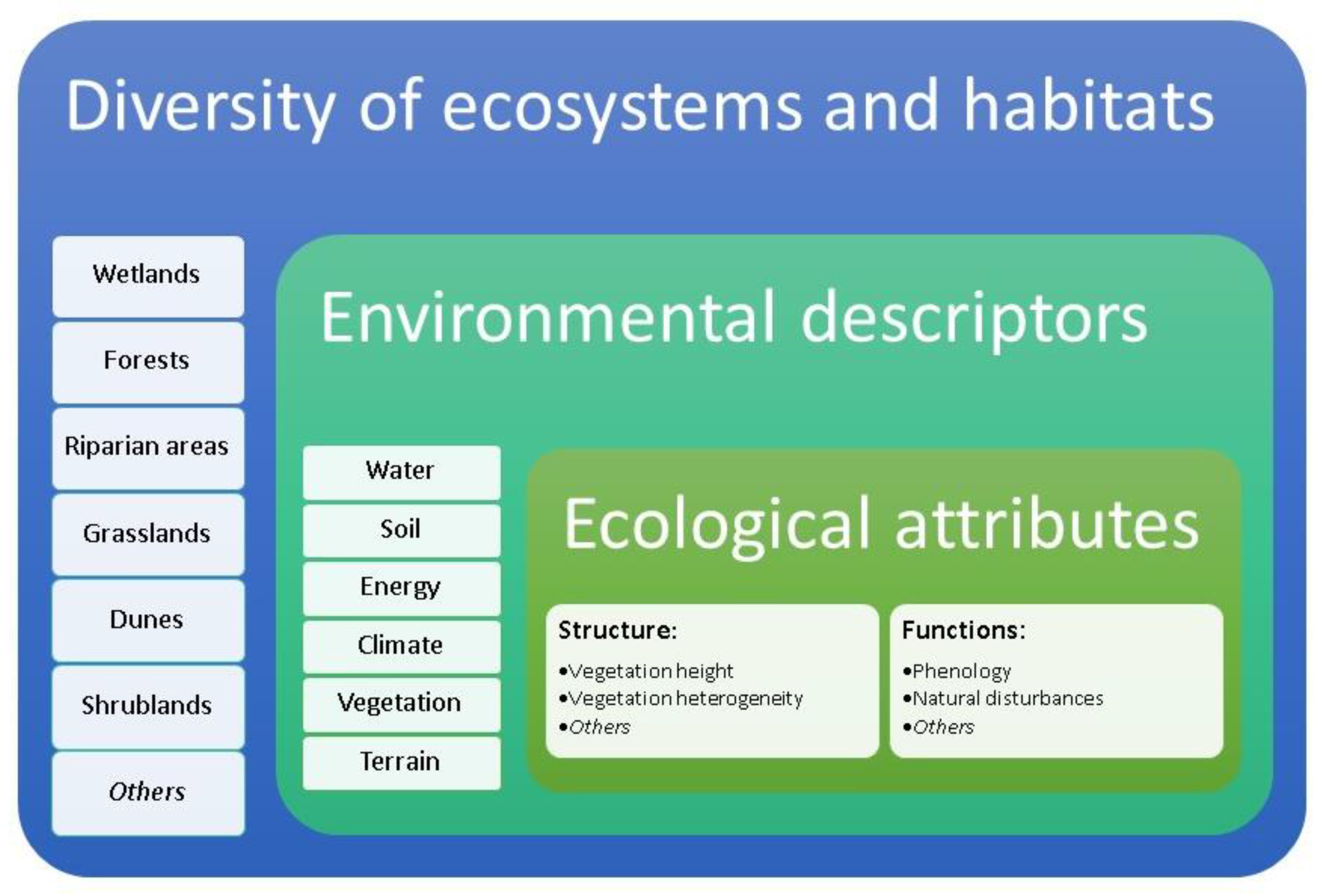
- The structural and functional attributes of ecosystems and habitats within PAs should be addressed;
- A broad set of variables representative of key biophysical quantitative descriptors should be used to produce integrated assessments, potentially including vegetation, energy, climate, water, terrain and soil.
- Global data sources presenting time series and regular updates should be preferred;
- Dimensionality reduction techniques are often used to deal with correlated input variables;
- The use of ensembles of different input data or models corresponding to the same variable is recommended to provide more accurate outputs and deal with uncertainty.
- The use of interoperable RS cloud-based infrastructures is recommended for large-scale processing;
- Analyses should be regularly repeated to document changes;
- The analysis should extend beyond specific habitat or ecosystem mapping and assessment methods so that a variety of habitats and ecosystem types can be identified;
- The resulting habitat and ecosystem types within PAs should be, to the greatest extent possible, comparable with existing global typologies;
- There is a clear need and potential to develop methodologies for assessing the biophysical uniqueness of PAs that could support prioritization analyses;
- Methods should allow the prediction of climate change impacts on ecosystems by using forecasted bioclimatic data.
- Translate the results into information that can be used by policy and decision-makers;
- Ensure transparency and reproducibility by sharing all data and models generated using online interoperable tools;
- Global characterization of PAs should be specifically aimed at informing larger scale conservation and management actions and plans, unless no better information is available at the local or regional scales.
Supplementary Materials
Author Contributions
Funding
Institutional Review Board Statement
Informed Consent Statement
Data Availability Statement
Acknowledgments
Conflicts of Interest
References
- Maxwell, S.L.; Cazalis, V.; Dudley, N.; Hoffmann, M.; Rodrigues, A.S.L.; Stolton, S.; Visconti, P.; Woodley, S.; Kingston, N.; Lewis, E.; et al. Area-based conservation in the twenty-first century. Nature 2020, 586, 217–227. [Google Scholar] [CrossRef]
- Mappin, B.; Chauvenet, A.L.M.; Adams, V.M.; Di Marco, M.; Beyer, H.L.; Venter, O.; Halpern, B.S.; Possingham, H.P.; Watson, J.E.M. Restoration priorities to achieve the global protected area target. Conserv. Lett. 2019, e12646. [Google Scholar] [CrossRef] [Green Version]
- Thomas, C.D.; Gillingham, P.K. The performance of protected areas for biodiversity under climate change. Biol. J. Linn. Soc. Lond. 2015, 115, 718–730. [Google Scholar] [CrossRef]
- Elsen, P.R.; Monahan, W.B.; Merenlender, A.M. Global patterns of protection of elevational gradients in mountain ranges. Proc. Natl. Acad. Sci. USA 2018, 115, 6004–6009. [Google Scholar] [CrossRef] [PubMed] [Green Version]
- Pascual, U.; Balvanera, P.; Díaz, S.; Pataki, G.; Roth, E.; Stenseke, M.; Watson, R.T.; Başak Dessane, E.; Islar, M.; Kelemen, E.; et al. Valuing nature’s contributions to people: The IPBES approach. Curr. Opin. Environ. Sustain. 2017, 26–27, 7–16. [Google Scholar] [CrossRef] [Green Version]
- Dinerstein, E.; Olson, D.; Joshi, A.; Vynne, C.; Burgess, N.D.; Wikramanayake, E.; Hahn, N.; Palminteri, S.; Hedao, P.; Noss, R.; et al. An Ecoregion-Based Approach to Protecting Half the Terrestrial Realm. Bioscience 2017, 67, 534–545. [Google Scholar] [CrossRef]
- Grêt-Regamey, A.; Weibel, B. Global assessment of mountain ecosystem services using earth observation data. Ecosyst. Serv. 2020, 46, 101213. [Google Scholar] [CrossRef]
- Cooper, G.S.; Willcock, S.; Dearing, J.A. Regime shifts occur disproportionately faster in larger ecosystems. Nat. Commun. 2020, 11, 1175. [Google Scholar] [CrossRef] [PubMed] [Green Version]
- EC. EU Biodiversity Strategy for 2030 Bringing Nature Back into Our Lives; (COM/2020/380 final); Official Journal of the European Union: Brussels, Belgium, 2020. [Google Scholar]
- Saarikoski, H.; Mustajoki, J.; Barton, D.N.; Geneletti, D.; Langemeyer, J.; Gomez-Baggethun, E.; Marttunen, M.; Antunes, P.; Keune, H.; Santos, R. Multi-Criteria Decision Analysis and Cost-Benefit Analysis: Comparing alternative frameworks for integrated valuation of ecosystem services. Ecosyst. Serv. 2016, 22, 238–249. [Google Scholar] [CrossRef]
- Belle, E.; Kingston, N.; Burgess, N.; Sandwith, T.; Ali, N.; MacKinnon, K. Protected Planet Report 2018: Tracking Progress Towards Global Targets for Protected Areas; UNEP-WCMC, IUCN and NGS: Cambridge, UK; Gland, Switzerland; Washington, DC, USA, 2018. [Google Scholar]
- Bonet-García, F.J.; Pérez-Luque, A.J.; Moreno-Llorca, R.A.; Pérez-Pérez, R.; Puerta-Piñero, C.; Zamora, R. Protected areas as elicitors of human well-being in a developed region: A new synthetic (socioeconomic) approach. Biol. Conserv. 2015, 187, 221–229. [Google Scholar] [CrossRef]
- Moreno-Llorca, R.; Vaz, A.S.; Herrero, J.; Millares, A.; Bonet-García, F.J.; Alcaraz-Segura, D. Multi-scale evolution of ecosystem services’ supply in Sierra Nevada (Spain): An assessment over the last half-century. Ecosyst. Serv. 2020, 46, 101204. [Google Scholar] [CrossRef]
- Naidoo, R.; Gerkey, D.; Hole, D.; Pfaff, A.; Ellis, A.M.; Golden, C.D.; Herrera, D.; Johnson, K.; Mulligan, M.; Ricketts, T.H.; et al. Evaluating the impacts of protected areas on human well-being across the developing world. Sci. Adv. 2019, 5, eaav3006. [Google Scholar] [CrossRef] [Green Version]
- Bunce, R.G.H.; Bogers, M.M.B.; Evans, D.; Halada, L.; Jongman, R.H.G.; Mucher, C.A.; Bauch, B.; de Blust, G.; Parr, T.W.; Olsvig-Whittaker, L. The significance of habitats as indicators of biodiversity and their links to species. Ecol. Indic. 2013, 33, 19–25. [Google Scholar] [CrossRef]
- Reid, W.V.; Mooney, H.A.; Cropper, A.; Capistrano, D.; Carpenter, S.R.; Chopra, K.; Dasgupta, P.; Dietz, T.; Duraiappah, A.K.; Hassan, R.; et al. Millennium Ecosystem Assessment. Ecosystems and Human Well-Being: Synthesis; Island Press: Washington, DC, USA, 2005. [Google Scholar]
- Jung, M.; Dahal, P.R.; Butchart, S.H.M.; Donald, P.F.; De Lamo, X.; Lesiv, M.; Kapos, V.; Rondinini, C.; Visconti, P. A global map of terrestrial habitat types. Sci. Data 2020, 7, 256. [Google Scholar] [CrossRef]
- Pereira, H.M.; Ferrier, S.; Walters, M.; Geller, G.N.; Jongman, R.H.G.; Scholes, R.J.; Bruford, M.W.; Brummitt, N.; Butchart, S.H.M.; Cardoso, A.C.; et al. Essential Biodiversity Variables. Science 2013, 339, 277–278. [Google Scholar] [CrossRef] [Green Version]
- Mairota, P.; Cafarelli, B.; Boccaccio, L.; Leronni, V.; Labadessa, R.; Kosmidou, V.; Nagendra, H. Using landscape structure to develop quantitative baselines for protected area monitoring. Ecol. Indic. 2013, 33, 82–95. [Google Scholar] [CrossRef]
- Dash, J.; Ogutu, B.O. Recent advances in space-borne optical remote sensing systems for monitoring global terrestrial ecosystems. Prog. Phys. Geogr. 2016, 40, 322–351. [Google Scholar] [CrossRef]
- Buchanan, G.M.; Beresford, A.E.; Hebblewhite, M.; Escobedo, F.J.; De Klerk, H.M.; Donald, P.F.; Escribano, P.; Koh, L.P.; Martínez-López, J.; Pettorelli, N.; et al. Free satellite data key to conservation. Science 2018, 361, 139–140. [Google Scholar] [CrossRef]
- Rose, R.A.; Byler, D.; Eastman, J.R.; Fleishman, E.; Geller, G.; Goetz, S.; Guild, L.; Hamilton, H.; Hansen, M.; Headley, R.; et al. Ten ways remote sensing can contribute to conservation. Conserv. Biol. 2015, 29, 350–359. [Google Scholar] [CrossRef] [Green Version]
- O’Connor, B.; Moul, K.; Pollini, B.; de Lamo, X.; Simonson, W.; Allison, H.; Albrecht, F.; Guzinski, R.M.; Larsen, H.; McGlade, J.; et al. Earth Observation for SDG—Compendium of Earth Observation Contributions to the SDG Targets and Indicators; European Space Agency: Paris, France, 2020; p. 165. [Google Scholar]
- Petrou, Z.I.; Manakos, I.; Stathaki, T. Remote sensing for biodiversity monitoring: A review of methods for biodiversity indicator extraction and assessment of progress towards international targets. Biodivers. Conserv. 2015, 24, 2333–2363. [Google Scholar] [CrossRef]
- Latombe, G.; Pyšek, P.; Jeschke, J.M.; Blackburn, T.M.; Bacher, S.; Capinha, C.; Costello, M.J.; Fernández, M.; Gregory, R.D.; Hobern, D.; et al. A vision for global monitoring of biological invasions. Biol. Conserv. 2017, 213, 295–308. [Google Scholar] [CrossRef]
- De Araujo Barbosa, C.C.; Atkinson, P.M.; Dearing, J.A. Remote sensing of ecosystem services: A systematic review. Ecol. Indic. 2015, 52, 430–443. [Google Scholar] [CrossRef]
- Dubovyk, O. The role of Remote Sensing in land degradation assessments: Opportunities and challenges. Eur. J. Remote Sens. 2017, 50, 601–613. [Google Scholar] [CrossRef]
- Wang, Y.; Yésou, H. Remote sensing of floodpath lakes and wetlands: A challenging frontier in the monitoring of changing environments. Remote Sens. 2018, 10, 1955. [Google Scholar] [CrossRef] [Green Version]
- Wang, Y.; Lu, Z.; Sheng, Y.; Zhou, Y. Remote sensing applications in monitoring of protected areas. Remote Sens. 2020, 12, 1370. [Google Scholar] [CrossRef]
- Mao, L.; Li, M.; Shen, W. Remote sensing applications for monitoring terrestrial protected areas: Progress in the last decade. Sustainability 2020, 12, 5016. [Google Scholar] [CrossRef]
- Pettorelli, N.; Wegmann, M.; Gurney, L.; Dubois, G. Monitoring Protected Areas from Space. In Protected Areas: Are They Safeguarding Biodiversity? Joppa, L.N., Baillie, J.E.M., Robinson, J.G., Eds.; John Wiley & Sons, Ltd.: Chichester, UK, 2016; pp. 242–259. [Google Scholar]
- Gillespie, T.W.; Willis, K.S.; Ostermann-Kelm, S. Spaceborne remote sensing of the world’s protected areas. Prog. Phys. Geogr. Earth Environ. 2015, 39, 388–404. [Google Scholar] [CrossRef]
- Duan, P.; Wang, Y.; Yin, P. Remote sensing applications in monitoring of protected areas: A bibliometric analysis. Remote Sens. 2020, 12, 772. [Google Scholar] [CrossRef] [Green Version]
- Tsyganskaya, V.; Martinis, S.; Marzahn, P. Flood Monitoring in Vegetated Areas Using Multitemporal Sentinel-1 Data: Impact of Time Series Features. Water 2019, 11, 1938. [Google Scholar] [CrossRef] [Green Version]
- Liu, C.-C.; Shieh, M.-C.; Ke, M.-S.; Wang, K.-H. Flood prevention and emergency response system powered by google earth engine. Remote Sens. 2018, 10, 1283. [Google Scholar] [CrossRef] [Green Version]
- Nemani, R.; Hashimoto, H.; Votava, P.; Melton, F.; Wang, W.; Michaelis, A.; Mutch, L.; Milesi, C.; Hiatt, S.; White, M. Monitoring and forecasting ecosystem dynamics using the Terrestrial Observation and Prediction System (TOPS). Remote Sens. Environ. 2009, 113, 1497–1509. [Google Scholar] [CrossRef]
- Wiens, J.; Sutter, R.; Anderson, M.; Blanchard, J.; Barnett, A.; Aguilar-Amuchastegui, N.; Avery, C.; Laine, S. Selecting and conserving lands for biodiversity: The role of remote sensing. Remote Sens. Environ. 2009, 113, 1370–1381. [Google Scholar] [CrossRef] [Green Version]
- Wilson, M.C.; Chen, X.-Y.; Corlett, R.T.; Didham, R.K.; Ding, P.; Holt, R.D.; Holyoak, M.; Hu, G.; Hughes, A.C.; Jiang, L.; et al. Habitat fragmentation and biodiversity conservation: Key findings and future challenges. Landsc. Ecol. 2016, 31, 219–227. [Google Scholar] [CrossRef] [Green Version]
- Wang, R.; Gamon, J.A. Remote sensing of terrestrial plant biodiversity. Remote Sens. Environ. 2019, 231, 111218. [Google Scholar] [CrossRef]
- Jetz, W.; Cavender-Bares, J.; Pavlick, R.; Schimel, D.; Davis, F.W.; Asner, G.P.; Guralnick, R.; Kattge, J.; Latimer, A.M.; Moorcroft, P.; et al. Monitoring plant functional diversity from space. Nat. Plants 2016, 2, 16024. [Google Scholar] [CrossRef] [PubMed] [Green Version]
- Rolf, W.; Lenz, R.; Peters, D. Development of a quantitative “bioassay” approach for ecosystem mapping. Int. J. Biodivers. Sci. Ecosyst. Serv. Manag. 2012, 8, 71–79. [Google Scholar] [CrossRef]
- Mücher, C.A.; Klijn, J.A.; Wascher, D.M.; Schaminée, J.H.J. A new European Landscape Classification (LANMAP): A transparent, flexible and user-oriented methodology to distinguish landscapes. Ecol. Indic. 2010, 10, 87–103. [Google Scholar] [CrossRef]
- Hargrove, W.W.; Hoffman, F.M. Potential of multivariate quantitative methods for delineation and visualization of ecoregions. Environ. Manag. 2004, 34 (Suppl. 1), S39–S60. [Google Scholar] [CrossRef]
- Metzger, M.J.; Bunce, R.G.H.; Jongman, R.H.G.; Mücher, C.A.; Watkins, J.W. A climatic stratification of the environment of Europe. Glob. Ecol. Biogeogr. 2005, 14, 549–563. [Google Scholar] [CrossRef]
- Sayre, R.; Comer, P.; Warner, H.; Cress, J. A New Map of Standardized Terrestrial Ecosystems of the Conterminous United States; U.S. Geological Survey Professional Paper; U.S. Geological Survey: Reston, VA, USA, 2009; p. 17. [Google Scholar]
- Felipe-Lucia, M.R.; Soliveres, S.; Penone, C.; Fischer, M.; Ammer, C.; Boch, S.; Boeddinghaus, R.S.; Bonkowski, M.; Buscot, F.; Fiore-Donno, A.M.; et al. Land-use intensity alters networks between biodiversity, ecosystem functions, and services. Proc. Natl. Acad. Sci. USA 2020, 117, 28140–28149. [Google Scholar] [CrossRef]
- Pettorelli, N.; Owen, H.J.F.; Duncan, C. How do we want Satellite Remote Sensing to support biodiversity conservation globally? Methods Ecol. Evol. 2016, 7, 656–665. [Google Scholar] [CrossRef]
- Skidmore, A.K.; Pettorelli, N.; Coops, N.C.; Geller, G.N.; Hansen, M.; Lucas, R.; Mücher, C.A.; O’Connor, B.; Paganini, M.; Pereira, H.M.; et al. Environmental science: Agree on biodiversity metrics to track from space. Nature 2015, 523, 403–405. [Google Scholar] [CrossRef] [Green Version]
- Vihervaara, P.; Mononen, L.; Auvinen, A.-P.; Virkkala, R.; Lü, Y.; Pippuri, I.; Packalen, P.; Valbuena, R.; Valkama, J. How to integrate remotely sensed data and biodiversity for ecosystem assessments at landscape scale. Landsc. Ecol. 2015, 30, 501–516. [Google Scholar] [CrossRef]
- Olson, D.M.; Dinerstein, E.; Wikramanayake, E.D.; Burgess, N.D.; Powell, G.V.N.; Underwood, E.C.; D’amico, J.A.; Itoua, I.; Strand, H.E.; Morrison, J.C.; et al. Terrestrial Ecoregions of the World: A New Map of Life on Earth: A new global map of terrestrial ecoregions provides an innovative tool for conserving biodiversity. BioScience 2001, 51, 933–938. [Google Scholar] [CrossRef]
- Sayre, R.; Karagulle, D.; Frye, C.; Boucher, T.; Wolff, N.H.; Breyer, S.; Wright, D.; Martin, M.; Butler, K.; Van Graafeiland, K.; et al. An assessment of the representation of ecosystems in global protected areas using new maps of World Climate Regions and World Ecosystems. Glob. Ecol. Conserv. 2020, 21, e00860. [Google Scholar] [CrossRef]
- Pérez-Hoyos, A.; Martínez, B.; García-Haro, F.; Moreno, Á.; Gilabert, M. Identification of Ecosystem Functional Types from Coarse Resolution Imagery Using a Self-Organizing Map Approach: A Case Study for Spain. Remote Sens. 2014, 6, 11391–11419. [Google Scholar] [CrossRef] [Green Version]
- Ivits, E.; Cherlet, M.; Horion, S.; Fensholt, R. Global biogeographical pattern of ecosystem functional types derived from earth observation data. Remote Sens. 2013, 5, 3305–3330. [Google Scholar] [CrossRef] [Green Version]
- Bastos, R.; Monteiro, A.T.; Carvalho, D.; Gomes, C.; Travassos, P.; Honrado, J.P.; Santos, M.; Cabral, J.A. Integrating land cover structure and functioning to predict biodiversity patterns: A hierarchical modelling framework designed for ecosystem management. Landsc. Ecol. 2016, 31, 701–710. [Google Scholar] [CrossRef]
- Nagendra, H.; Lucas, R.; Honrado, J.P.; Jongman, R.H.G.; Tarantino, C.; Adamo, M.; Mairota, P. Remote sensing for conservation monitoring: Assessing protected areas, habitat extent, habitat condition, species diversity, and threats. Ecol. Indic. 2013, 33, 45–59. [Google Scholar] [CrossRef]
- Corbane, C.; Lang, S.; Pipkins, K.; Alleaume, S.; Deshayes, M.; García Millán, V.E.; Strasser, T.; Vanden Borre, J.; Toon, S.; Michael, F. Remote sensing for mapping natural habitats and their conservation status—New opportunities and challenges. Int. J. Appl. Earth Obs. Geoinf. 2015, 37, 7–16. [Google Scholar] [CrossRef]
- Villoslada, M.; Bunce, R.G.H.; Sepp, K.; Jongman, R.H.G.; Metzger, M.J.; Kull, T.; Raet, J.; Kuusemets, V.; Kull, A.; Leito, A. A framework for habitat monitoring and climate change modelling: Construction and validation of the Environmental Stratification of Estonia. Reg. Environ. Chang. 2017, 17, 335–349. [Google Scholar] [CrossRef] [Green Version]
- Jongman, R.H.G.; Mücher, C.A.; Bunce, R.G.H.; Lang, M.; Sepp, K. A Review of Approaches for Automated Habitat Mapping and their Potential Added Value for Biodiversity Monitoring Projects. J. Landsc. Ecol. 2019, 12, 53–69. [Google Scholar] [CrossRef] [Green Version]
- Lang, M.; Vain, A.; Bunce, R.G.H.; Jongman, R.H.G.; Raet, J.; Sepp, K.; Kuusemets, V.; Kikas, T.; Liba, N. Extrapolation of in situ data from 1-km squares to adjacent squares using remote sensed imagery and airborne lidar data for the assessment of habitat diversity and extent. Environ. Monit. Assess. 2015, 187, 76. [Google Scholar] [CrossRef] [PubMed]
- Vaz, A.S.; Marcos, B.; Gonçalves, J.; Monteiro, A.; Alves, P.; Civantos, E.; Lucas, R.; Mairota, P.; Garcia-Robles, J.; Alonso, J.; et al. Can we predict habitat quality from space? A multi-indicator assessment based on an automated knowledge-driven system. Int. J. Appl. Earth Obs. Geoinf. 2015, 37, 106–113. [Google Scholar] [CrossRef]
- Mairota, P.; Cafarelli, B.; Didham, R.K.; Lovergine, F.P.; Lucas, R.M.; Nagendra, H.; Rocchini, D.; Tarantino, C. Challenges and opportunities in harnessing satellite remote-sensing for biodiversity monitoring. Ecol. Inform. 2015, 30, 207–214. [Google Scholar] [CrossRef]
- Pettorelli, N.; Schulte to Bühne, H.; Tulloch, A.; Dubois, G.; Macinnis-Ng, C.; Queirós, A.M.; Keith, D.A.; Wegmann, M.; Schrodt, F.; Stellmes, M.; et al. Satellite remote sensing of ecosystem functions: Opportunities, challenges and way forward. Remote Sens. Ecol. Conserv. 2017, 4, 1–23. [Google Scholar] [CrossRef]
- Chatziantoniou, A.; Psomiadis, E.; Petropoulos, G. Co-Orbital Sentinel 1 and 2 for LULC Mapping with Emphasis on Wetlands in a Mediterranean Setting Based on Machine Learning. Remote Sens. 2017, 9, 1259. [Google Scholar] [CrossRef] [Green Version]
- Chavez, L.J. Identifying Dune Habitat through the Use of Remote Sensing Classifications. Ph.D. Thesis, Texas State University, San Marcos, TA, USA, 2019. [Google Scholar]
- Mao, D.; Wang, Z.; Du, B.; Li, L.; Tian, Y.; Jia, M.; Zeng, Y.; Song, K.; Jiang, M.; Wang, Y. National wetland mapping in China: A new product resulting from object-based and hierarchical classification of Landsat 8 OLI images. ISPRS J. Photogramm. Remote Sens. 2020, 164, 11–25. [Google Scholar] [CrossRef]
- Campbell, A.; Wang, Y. High spatial resolution remote sensing for salt marsh mapping and change analysis at fire island national seashore. Remote Sens. 2019, 11, 1107. [Google Scholar] [CrossRef] [Green Version]
- Szantoi, Z.; Escobedo, F.J.; Abd-Elrahman, A.; Pearlstine, L.; Dewitt, B.; Smith, S. Classifying spatially heterogeneous wetland communities using machine learning algorithms and spectral and textural features. Environ. Monit. Assess. 2015, 187, 262. [Google Scholar] [CrossRef] [PubMed]
- Kollár, S.; Vekerdy, Z.; Márkus, B. Forest habitat change dynamics in a riparian wetland. Procedia Environ. Sci. 2011, 7, 371–376. [Google Scholar] [CrossRef] [Green Version]
- Szantoi, Z.; Escobedo, F.; Abd-Elrahman, A.; Smith, S.; Pearlstine, L. Analyzing fine-scale wetland composition using high resolution imagery and texture features. Int. J. Appl. Earth Obs. Geoinf. 2013, 23, 204–212. [Google Scholar] [CrossRef]
- Lane, C.; Liu, H.; Autrey, B.; Anenkhonov, O.; Chepinoga, V.; Wu, Q. Improved Wetland Classification Using Eight-Band High Resolution Satellite Imagery and a Hybrid Approach. Remote Sens. 2014, 6, 12187–12216. [Google Scholar] [CrossRef] [Green Version]
- Strasser, T.; Lang, S. Object-based class modelling for multi-scale riparian forest habitat mapping. Int. J. Appl. Earth Obs. Geoinf. 2015, 37, 29–37. [Google Scholar] [CrossRef]
- Johansen, K.; Coops, N.C.; Gergel, S.E.; Stange, Y. Application of high spatial resolution satellite imagery for riparian and forest ecosystem classification. Remote Sens. Environ. 2007, 110, 29–44. [Google Scholar] [CrossRef]
- Wendelberger, K.S.; Gann, D.; Richards, J.H. Using Bi-Seasonal WorldView-2 Multi-Spectral Data and Supervised Random Forest Classification to Map Coastal Plant Communities in Everglades National Park. Sensors 2018, 18, 829. [Google Scholar] [CrossRef] [PubMed] [Green Version]
- Rapinel, S.; Mony, C.; Lecoq, L.; Clément, B.; Thomas, A.; Hubert-Moy, L. Evaluation of Sentinel-2 time-series for mapping floodplain grassland plant communities. Remote Sens. Environ. 2019, 223, 115–129. [Google Scholar] [CrossRef]
- Zhang, L.; Li, X.; Lu, S.; Jia, K. Multi-scale object-based measurement of arid plant community structure. Int. J. Remote Sens. 2016, 37, 2168–2179. [Google Scholar] [CrossRef]
- Silveyra Gonzalez, R.; Latifi, H.; Weinacker, H.; Dees, M.; Koch, B.; Heurich, M. Integrating LiDAR and high-resolution imagery for object-based mapping of forest habitats in a heterogeneous temperate forest landscape. Int. J. Remote Sens. 2018, 39, 8859–8884. [Google Scholar] [CrossRef]
- Stabach, J.A.; Dabek, L.; Jensen, R.; Wang, Y.Q. Discrimination of dominant forest types for Matschie’s tree kangaroo conservation in Papua New Guinea using high-resolution remote sensing data. Int. J. Remote Sens. 2009, 30, 405–422. [Google Scholar] [CrossRef]
- Marselis, S.M.; Abernethy, K.; Alonso, A.; Armston, J.; Baker, T.R.; Bastin, J.; Bogaert, J.; Boyd, D.S.; Boeckx, P.; Burslem, D.F.R.P.; et al. Evaluating the potential of full-waveform lidar for mapping pan-tropical tree species richness. Glob. Ecol. Biogeogr. 2020. [Google Scholar] [CrossRef]
- Jiménez López, J.; Mulero-Pázmány, M. Drones for conservation in protected areas: Present and future. Drones 2019, 3, 10. [Google Scholar] [CrossRef] [Green Version]
- Onojeghuo, A.O.; Blackburn, G.A. Optimising the use of hyperspectral and LiDAR data for mapping reedbed habitats. Remote Sens. Environ. 2011, 115, 2025–2034. [Google Scholar] [CrossRef]
- Guo, X.; Coops, N.C.; Tompalski, P.; Nielsen, S.E.; Bater, C.W.; John Stadt, J. Regional mapping of vegetation structure for biodiversity monitoring using airborne lidar data. Ecol. Inform. 2017, 38, 50–61. [Google Scholar] [CrossRef]
- Cheţan, M.A.; Dornik, A. 20 years of landscape dynamics within the world’s largest multinational network of protected areas. J. Environ. Manag. 2020, 111712. [Google Scholar] [CrossRef]
- Mairota, P.; Cafarelli, B.; Labadessa, R.; Lovergine, F.; Tarantino, C.; Lucas, R.M.; Nagendra, H.; Didham, R.K. Very high resolution Earth observation features for monitoring plant and animal community structure across multiple spatial scales in protected areas. Int. J. Appl. Earth Obs. Geoinf. 2015, 37, 100–105. [Google Scholar] [CrossRef]
- Park, Y.; Guldmann, J.-M. Measuring continuous landscape patterns with Gray-Level Co-Occurrence Matrix (GLCM) indices: An alternative to patch metrics? Ecol. Indic. 2020, 109, 105802. [Google Scholar] [CrossRef]
- Ozdemir, I.; Mert, A.; Ozkan, U.Y.; Aksan, S.; Unal, Y. Predicting bird species richness and micro-habitat diversity using satellite data. For. Ecol. Manag. 2018, 424, 483–493. [Google Scholar] [CrossRef]
- St-Louis, V.; Pidgeon, A.M.; Clayton, M.K.; Locke, B.A.; Bash, D.; Radeloff, V.C. Satellite image texture and a vegetation index predict avian biodiversity in the Chihuahuan Desert of New Mexico. Ecography 2009, 32, 468–480. [Google Scholar] [CrossRef]
- Wood, E.M.; Pidgeon, A.M.; Radeloff, V.C.; Keuler, N.S. Image texture as a remotely sensed measure of vegetation structure. Remote Sens. Environ. 2012, 121, 516–526. [Google Scholar] [CrossRef]
- Farwell, L.S.; Elsen, P.R.; Razenkova, E.; Pidgeon, A.M.; Radeloff, V.C. Habitat heterogeneity captured by 30-m resolution satellite image texture predicts bird richness across the United States. Ecol. Appl. 2020, 30, e02157. [Google Scholar] [CrossRef] [PubMed]
- Farwell, L.S.; Gudex-Cross, D.; Anise, I.E.; Bosch, M.J.; Olah, A.M.; Radeloff, V.C.; Razenkova, E.; Rogova, N.; Silveira, E.M.O.; Smith, M.M.; et al. Satellite image texture captures vegetation heterogeneity and explains patterns of bird richness. Remote Sens. Environ. 2021, 253, 112175. [Google Scholar] [CrossRef]
- Hobi, M.L.; Dubinin, M.; Graham, C.H.; Coops, N.C.; Clayton, M.K.; Pidgeon, A.M.; Radeloff, V.C. A comparison of Dynamic Habitat Indices derived from different MODIS products as predictors of avian species richness. Remote Sens. Environ. 2017, 195, 142–152. [Google Scholar] [CrossRef]
- Berry, S.; Mackey, B.; Brown, T. Potential applications of remotely sensed vegetation greenness to habitat analysis and the conservation of dispersive fauna. Pac. Conserv. Biol. 2007, 13, 120. [Google Scholar] [CrossRef]
- Madonsela, S.; Cho, M.A.; Ramoelo, A.; Mutanga, O. Remote sensing of species diversity using Landsat 8 spectral variables. ISPRS J. Photogramm. Remote Sens. 2017, 133, 116–127. [Google Scholar] [CrossRef] [Green Version]
- Ribeiro, I.; Proença, V.; Serra, P.; Palma, J.; Domingo-Marimon, C.; Pons, X.; Domingos, T. Remotely sensed indicators and open-access biodiversity data to assess bird diversity patterns in Mediterranean rural landscapes. Sci. Rep. 2019, 9, 6826. [Google Scholar] [CrossRef] [PubMed] [Green Version]
- Chu, T.; Guo, X.; Takeda, K. Remote sensing approach to detect post-fire vegetation regrowth in Siberian boreal larch forest. Ecol. Indic. 2016, 62, 32–46. [Google Scholar] [CrossRef]
- Fernandez-Manso, A.; Quintano, C.; Roberts, D.A. Burn severity influence on post-fire vegetation cover resilience from Landsat MESMA fraction images time series in Mediterranean forest ecosystems. Remote Sens. Environ. 2016, 184, 112–123. [Google Scholar] [CrossRef]
- Alcaraz, D.; Paruelo, J.; Cabello, J. Identification of current ecosystem functional types in the Iberian Peninsula. Glob. Ecol. Biogeogr. 2006, 15, 200–212. [Google Scholar] [CrossRef]
- Schirpke, U.; Leitinger, G.; Tasser, E.; Rüdisser, J.; Fontana, V.; Tappeiner, U. Functional spatial units are fundamental for modelling ecosystem services in mountain regions. Appl. Geogr. 2020, 118, 102200. [Google Scholar] [CrossRef]
- Keith, D.A.; Rodríguez, J.P.; Rodríguez-Clark, K.M.; Nicholson, E.; Aapala, K.; Alonso, A.; Asmussen, M.; Bachman, S.; Basset, A.; Barrow, E.G.; et al. Scientific foundations for an IUCN Red List of ecosystems. PLoS ONE 2013, 8, e62111. [Google Scholar] [CrossRef] [Green Version]
- Xie, Y.; Sha, Z.; Yu, M. Remote sensing imagery in vegetation mapping: A review. J. Plant Ecol. 2008, 1, 9–23. [Google Scholar] [CrossRef]
- Hijmans, R.J.; Cameron, S.E.; Parra, J.L.; Jones, P.G.; Jarvis, A. Very high resolution interpolated climate surfaces for global land areas. Int. J. Climatol. 2005, 25, 1965–1978. [Google Scholar] [CrossRef]
- Fick, S.E.; Hijmans, R.J. WorldClim 2: New 1-km spatial resolution climate surfaces for global land areas. Int. J. Climatol. 2017, 37, 4302–4315. [Google Scholar] [CrossRef]
- Holdridge, L.R. Life Zone Ecology; Tropical Science Center: San Jose, CA, USA, 1967; p. 206. [Google Scholar]
- Beck, H.E.; Zimmermann, N.E.; McVicar, T.R.; Vergopolan, N.; Berg, A.; Wood, E.F. Present and future Köppen-Geiger climate classification maps at 1-km resolution. Sci. Data 2018, 5, 180214. [Google Scholar] [CrossRef] [PubMed] [Green Version]
- Amatulli, G.; Domisch, S.; Tuanmu, M.-N.; Parmentier, B.; Ranipeta, A.; Malczyk, J.; Jetz, W. A suite of global, cross-scale topographic variables for environmental and biodiversity modeling. Sci. Data 2018, 5, 180040. [Google Scholar] [CrossRef] [Green Version]
- Körner, C.; Paulsen, J.; Spehn, E.M. A definition of mountains and their bioclimatic belts for global comparisons of biodiversity data. Alp. Bot. 2011, 121, 73–78. [Google Scholar] [CrossRef] [Green Version]
- Linke, S.; Lehner, B.; Ouellet Dallaire, C.; Ariwi, J.; Grill, G.; Anand, M.; Beames, P.; Burchard-Levine, V.; Maxwell, S.; Moidu, H.; et al. Global hydro-environmental sub-basin and river reach characteristics at high spatial resolution. Sci. Data 2019, 6, 283. [Google Scholar] [CrossRef] [Green Version]
- Gao, H. Satellite remote sensing of large lakes and reservoirs: From elevation and area to storage. WIREs Water 2015, 2, 147–157. [Google Scholar] [CrossRef]
- Pickens, A.H.; Hansen, M.C.; Hancher, M.; Stehman, S.V.; Tyukavina, A.; Potapov, P.; Marroquin, B.; Sherani, Z. Mapping and sampling to characterize global inland water dynamics from 1999 to 2018 with full Landsat time-series. Remote Sens. Environ. 2020, 243, 111792. [Google Scholar] [CrossRef]
- Li, Z.-L.; Tang, B.-H.; Wu, H.; Ren, H.; Yan, G.; Wan, Z.; Trigo, I.F.; Sobrino, J.A. Satellite-derived land surface temperature: Current status and perspectives. Remote Sens. Environ. 2013, 131, 14–37. [Google Scholar] [CrossRef] [Green Version]
- Beach, T.; Luzzadder-Beach, S.; Dunning, N.P. Out of the Soil: Soil (Dark Matter Biodiversity) and Societal “Collapses” from Mesoamerica to Mesopotamia and Beyond. In Biological Extinction: New Perspectives; Dasgupta, P., Raven, P., McIvor, A., Eds.; Cambridge University Press: Cambridge, UK, 2019; pp. 138–174. [Google Scholar]
- Drobnik, T.; Schwaab, J.; Grêt-Regamey, A. Moving towards integrating soil into spatial planning: No net loss of soil-based ecosystem services. J. Environ. Manag. 2020, 263, 110406. [Google Scholar] [CrossRef] [PubMed]
- Smith, P.; Soussana, J.-F.; Angers, D.; Schipper, L.; Chenu, C.; Rasse, D.P.; Batjes, N.H.; van Egmond, F.; McNeill, S.; Kuhnert, M.; et al. How to measure, report and verify soil carbon change to realize the potential of soil carbon sequestration for atmospheric greenhouse gas removal. Glob. Chang. Biol. 2020, 26, 219–241. [Google Scholar] [CrossRef] [PubMed] [Green Version]
- Shoshany, M.; Goldshleger, N.; Chudnovsky, A. Monitoring of agricultural soil degradation by remote-sensing methods: A review. Int. J. Remote Sens. 2013, 34, 6152–6181. [Google Scholar] [CrossRef]
- Delgado-Baquerizo, M.; Maestre, F.T.; Reich, P.B.; Trivedi, P.; Osanai, Y.; Liu, Y.-R.; Hamonts, K.; Jeffries, T.C.; Singh, B.K. Carbon content and climate variability drive global soil bacterial diversity patterns. Ecol. Monogr. 2016, 86, 373–390. [Google Scholar] [CrossRef]
- Fierer, N.; Jackson, R.B. The diversity and biogeography of soil bacterial communities. Proc. Natl. Acad. Sci. USA 2006, 103, 626–631. [Google Scholar] [CrossRef] [Green Version]
- Bastida, F.; Eldridge, D.J.; García, C.; Kenny Png, G.; Bardgett, R.D.; Delgado-Baquerizo, M. Soil microbial diversity-biomass relationships are driven by soil carbon content across global biomes. ISME J. 2021. [Google Scholar] [CrossRef]
- Siciliano, S.D.; Palmer, A.S.; Winsley, T.; Lamb, E.; Bissett, A.; Brown, M.V.; van Dorst, J.; Ji, M.; Ferrari, B.C.; Grogan, P.; et al. Soil fertility is associated with fungal and bacterial richness, whereas pH is associated with community composition in polar soil microbial communities. Soil Biol. Biochem. 2014, 78, 10–20. [Google Scholar] [CrossRef]
- Maestre, F.T.; Delgado-Baquerizo, M.; Jeffries, T.C.; Eldridge, D.J.; Ochoa, V.; Gozalo, B.; Quero, J.L.; García-Gómez, M.; Gallardo, A.; Ulrich, W.; et al. Increasing aridity reduces soil microbial diversity and abundance in global drylands. Proc. Natl. Acad. Sci. USA 2015, 112, 15684–15689. [Google Scholar] [CrossRef] [Green Version]
- Weil, R.R.; Brady, N.C. Nature and Properties of Soils, 15th ed.; Pearson Education: London, UK, 2016; p. 192. [Google Scholar]
- Martínez-López, J.; Bertzky, B.; Bonet-García, F.; Bastin, L.; Dubois, G. Biophysical Characterization of Protected Areas Globally through Optimized Image Segmentation and Classification. Remote Sens. 2016, 8, 780. [Google Scholar] [CrossRef] [Green Version]
- Pessôa, A.C.M.; Anderson, L.O.; Carvalho, N.S.; Campanharo, W.A.; Junior, C.H.L.S.; Rosan, T.M.; Reis, J.B.C.; Pereira, F.R.S.; Assis, M.; Jacon, A.D.; et al. Intercomparison of burned area products and its implication for carbon emission estimations in the amazon. Remote Sens. 2020, 12, 3864. [Google Scholar] [CrossRef]
- Chen, F.; Crow, W.T.; Ciabatta, L.; Filippucci, P.; Panegrossi, G.; Marra, A.C.; Puca, S.; Massari, C. Enhanced Large-Scale Validation of Satellite-Based Land Rainfall Products. J. Hydrometeor 2021, 22, 245–257. [Google Scholar] [CrossRef]
- Cunningham, D.; Cunningham, P.; Fagan, M.E. Identifying biases in global tree cover products: A case study in costa rica. Forests 2019, 10, 853. [Google Scholar] [CrossRef] [Green Version]
- Willcock, S.; Hooftman, D.A.P.; Blanchard, R.; Dawson, T.P.; Hickler, T.; Lindeskog, M.; Martinez-Lopez, J.; Reyers, B.; Watts, S.M.; Eigenbrod, F.; et al. Ensembles of ecosystem service models can improve accuracy and indicate uncertainty. Sci. Total Environ. 2020, 747, 141006. [Google Scholar] [CrossRef]
- Tuanmu, M.-N.; Jetz, W. A global 1-km consensus land-cover product for biodiversity and ecosystem modelling. Glob. Ecol. Biogeogr. 2014, 23, 1031–1045. [Google Scholar] [CrossRef]
- Muller-Karger, F.E.; Miloslavich, P.; Bax, N.J.; Simmons, S.; Costello, M.J.; Sousa Pinto, I.; Canonico, G.; Turner, W.; Gill, M.; Montes, E.; et al. Advancing marine biological observations and data requirements of the complementary essential ocean variables (eovs) and essential biodiversity variables (ebvs) frameworks. Front. Mar. Sci. 2018, 5. [Google Scholar] [CrossRef]
- Muller-Karger, F.E.; Hestir, E.; Ade, C.; Turpie, K.; Roberts, D.A.; Siegel, D.; Miller, R.J.; Humm, D.; Izenberg, N.; Keller, M.; et al. Satellite sensor requirements for monitoring essential biodiversity variables of coastal ecosystems. Ecol. Appl. 2018, 28, 749–760. [Google Scholar] [CrossRef] [PubMed]
- Miloslavich, P.; Bax, N.J.; Simmons, S.E.; Klein, E.; Appeltans, W.; Aburto-Oropeza, O.; Andersen Garcia, M.; Batten, S.D.; Benedetti-Cecchi, L.; Checkley, D.M.; et al. Essential ocean variables for global sustained observations of biodiversity and ecosystem changes. Glob. Chang. Biol. 2018. [Google Scholar] [CrossRef]
- El Mahrad, B.; Newton, A.; Icely, J.D.; Kacimi, I.; Abalansa, S.; Snoussi, M. Contribution of remote sensing technologies to a holistic coastal and marine environmental management framework: A review. Remote Sens. 2020, 12, 2313. [Google Scholar] [CrossRef]
- Kachelriess, D.; Wegmann, M.; Gollock, M.; Pettorelli, N. The application of remote sensing for marine protected area management. Ecol. Indic. 2014, 36, 169–177. [Google Scholar] [CrossRef]
- Wilson, A.M.; Jetz, W. Remotely Sensed High-Resolution Global Cloud Dynamics for Predicting Ecosystem and Biodiversity Distributions. PLoS Biol. 2016, 14, e1002415. [Google Scholar] [CrossRef] [PubMed]
- Tansey, K.; Grégoire, J.-M.; Defourny, P.; Leigh, R.; Pekel, J.-F.; van Bogaert, E.; Bartholomé, E. A new, global, multi-annual (2000–2007) burnt area product at 1 km resolution. Geophys. Res. Lett. 2008, 35. [Google Scholar] [CrossRef]
- Giglio, L.; Csiszar, I.; Justice, C.O. Global distribution and seasonality of active fires as observed with the Terra and Aqua Moderate Resolution Imaging Spectroradiometer (MODIS) sensors. J. Geophys. Res. 2006, 111. [Google Scholar] [CrossRef]
- Carmona-Moreno, C.; Belward, A.; Malingreau, J.-P.; Hartley, A.; Garcia-Alegre, M.; Antonovskiy, M.; Buchshtaber, V.; Pivovarov, V. Characterizing interannual variations in global fire calendar using data from Earth observing satellites. Glob. Chang. Biol. 2005, 11, 1537–1555. [Google Scholar] [CrossRef]
- Potapov, P.; Li, X.; Hernandez-Serna, A.; Tyukavina, A.; Hansen, M.C.; Kommareddy, A.; Pickens, A.; Turubanova, S.; Tang, H.; Silva, C.E.; et al. Mapping global forest canopy height through integration of GEDI and Landsat data. Remote Sens. Environ. 2020, 112165. [Google Scholar] [CrossRef]
- Lehner, B.; Grill, G. Global river hydrography and network routing: Baseline data and new approaches to study the world’s large river systems. Hydrol. Process. 2013, 27, 2171–2186. [Google Scholar] [CrossRef]
- Hansen, M.C.; Potapov, P.V.; Moore, R.; Hancher, M.; Turubanova, S.A.; Tyukavina, A.; Thau, D.; Stehman, S.V.; Goetz, S.J.; Loveland, T.R.; et al. High-resolution global maps of 21st-century forest cover change. Science 2013, 342, 850–853. [Google Scholar] [CrossRef] [PubMed] [Green Version]
- Ermida, S.L.; Soares, P.; Mantas, V.; Göttsche, F.-M.; Trigo, I.F. Google Earth Engine Open-Source Code for Land Surface Temperature Estimation from the Landsat Series. Remote Sens. 2020, 12, 1471. [Google Scholar] [CrossRef]
- Metzger, M.J.; Bunce, R.G.H.; Jongman, R.H.G.; Sayre, R.; Trabucco, A.; Zomer, R. A high-resolution bioclimate map of the world: A unifying framework for global biodiversity research and monitoring. Glob. Ecol. Biogeogr. 2013, 22, 630–638. [Google Scholar] [CrossRef] [Green Version]
- Sayre, R.; Dangermond, J.; Frye, C.; Vaughan, R.; Aniello, P.; Breyer, S.; Cribbs, D.; Hopkins, D.; Naumann, R.; Derrenbacher, B. A New Map of Global Ecological Land Units: An Ecophysiographic Stratification Approach; American Association Of Geographers: Washington, DC, USA, 2014; p. 46. [Google Scholar]
- Tuanmu, M.-N.; Jetz, W. A global, remote sensing-based characterization of terrestrial habitat heterogeneity for biodiversity and ecosystem modelling. Glob. Ecol. Biogeogr. 2015, 24, 1329–1339. [Google Scholar] [CrossRef]
- Huete, A.; Didan, K.; Miura, T.; Rodriguez, E.P.; Gao, X.; Ferreira, L.G. Overview of the radiometric and biophysical performance of the MODIS vegetation indices. Remote Sens. Environ. 2002, 83, 195–213. [Google Scholar] [CrossRef]
- Keith, D.A.; Ferrer-Paris, J.R.; Nicholson, E.; Kingsford, R.T. (Eds.) IUCN Global Ecosystem Typology 2.0: Descriptive Profiles for Biomes and Ecosystem Functional Groups; IUCN, International Union for Conservation of Nature: Gland, Switzerland, 2020. [Google Scholar]
- Lucas, R.; Blonda, P.; Bunting, P.; Jones, G.; Inglada, J.; Arias, M.; Kosmidou, V.; Petrou, Z.I.; Manakos, I.; Adamo, M.; et al. The Earth Observation Data for Habitat Monitoring (EODHaM) system. Int. J. Appl. Earth Obs. Geoinf. 2015, 37, 17–28. [Google Scholar] [CrossRef]
- Dubois, G.; Bastin, L.; Bertzky, B.; Mandrici, A.; Conti, M.; Saura, S.; Cottam, A.; Battistella, L.; Martínez-López, J.; Boni, M.; et al. Integrating Multiple Spatial Datasets to Assess Protected Areas: Lessons Learnt from the Digital Observatory for Protected Areas (DOPA). ISPRS Int. J. Geoinf. 2016, 5, 242. [Google Scholar] [CrossRef] [Green Version]
- Brink, A.; Martínez-López, J.; Szantoi, Z.; Moreno-Atencia, P.; Lupi, A.; Bastin, L.; Dubois, G. Indicators for assessing habitat values and pressures for protected areas—An integrated habitat and land cover change approach for the udzungwa mountains national park in tanzania. Remote Sens. 2016, 8, 862. [Google Scholar] [CrossRef] [Green Version]
- Dubois, G.; Schulz, M.; Skøien, J.; Bastin, L.; Peedell, S. eHabitat, a multi-purpose Web Processing Service for ecological modeling. Environ. Model. Softw. 2013, 41, 123–133. [Google Scholar] [CrossRef] [Green Version]
- Dubois, G.; Bastin, L.; Martínez-López, J.; Cottam, A.; Temperley, W.; Bertzky, B.; Graziano, M. The Digital Observatory for Protected Areas (DOPA) Explorer 1.0; EUR 27162 EN, Publications Office of the European Union: Luxembourg, 2015. [Google Scholar]
- Hoffmann, S.; Beierkuhnlein, C.; Field, R.; Provenzale, A.; Chiarucci, A. Uniqueness of protected areas for conservation strategies in the european union. Sci. Rep. 2018, 8, 6445. [Google Scholar] [CrossRef]
- Ejrnæs, R.; Frøslev, T.G.; Høye, T.T.; Kjøller, R.; Oddershede, A.; Brunbjerg, A.K.; Hansen, A.J.; Bruun, H.H. Uniquity: A general metric for biotic uniqueness of sites. Biol. Conserv. 2018, 225, 98–105. [Google Scholar] [CrossRef]
- Forero-Medina, G.; Joppa, L. Representation of global and national conservation priorities by Colombia’s Protected Area Network. PLoS ONE 2010, 5, e13210. [Google Scholar] [CrossRef]
- Martínez-López, J.; Bergillos, R.J.; Bonet, F.J.; de Vente, J. Connecting research infrastructures, scientific and sectorial networks to support integrated management of Mediterranean coastal and rural areas. Environ. Res. Lett. 2019, 14, 115001. [Google Scholar] [CrossRef]
- Bennett, M.K.; Younes, N.; Joyce, K. Automating drone image processing to map coral reef substrates using google earth engine. Drones 2020, 4, 50. [Google Scholar] [CrossRef]
- Ospina-Alvarez, A.; de Juan, S.; Davis, K.J.; González, C.; Fernández, M.; Navarrete, S.A. Integration of biophysical connectivity in the spatial optimization of coastal ecosystem services. Sci. Total Environ. 2020, 733, 139367. [Google Scholar] [CrossRef]
- Giardino, C.; Brando, V.E.; Gege, P.; Pinnel, N.; Hochberg, E.; Knaeps, E.; Reusen, I.; Doerffer, R.; Bresciani, M.; Braga, F.; et al. Imaging spectrometry of inland and coastal waters: State of the art, achievements and perspectives. Surv. Geophys. 2018, 40, 1–29. [Google Scholar] [CrossRef] [Green Version]
- de la Fuente, B.; Bertzky, B.; Delli, G.; Mandrici, A.; Conti, M.; Florczyk, A.J.; Freire, S.; Schiavina, M.; Bastin, L.; Dubois, G. Built-up areas within and around protected areas: Global patterns and 40-year trends. Glob. Ecol. Conserv. 2020, 24, e01291. [Google Scholar] [CrossRef] [PubMed]
- Willcock, S.; Hooftman, D.A.P.; Balbi, S.; Blanchard, R.; Dawson, T.P.; O’Farrell, P.J.; Hickler, T.; Hudson, M.D.; Lindeskog, M.; Martinez-Lopez, J.; et al. A Continental-Scale Validation of Ecosystem Service Models. Ecosystems 2019, 1–16. [Google Scholar] [CrossRef] [Green Version]
- Keith, D.A.; Ferrer-Paris, J.R.; Nicholson, E.; Bishop, M.J.; Polidoro, B.A.; Ramirez-Llodra, E.; Tozer, M.G.; Nel, J.L.; Mac Nally, R.; Gregr, E.J.; et al. Indicative distribution maps for Ecosystem Functional Groups—Level 3 of IUCN Global Ecosystem Typology. Zenodo 2020. [Google Scholar] [CrossRef]
- Lightfoot, P. Object-Based Mapping of Temperate Marine Habitats from Multi-Resolution Remote Sensing Data. Ph.D. Thesis, Newcastle University, Newcastle, UK, 2018. [Google Scholar]
- Sagar, S.; Falkner, I.; Dekker, A.; Huang, Z.; Blondeau-Patissier, D.; Phillips, C.; Przeslawski, R. Earth Observation for monitoring of Australian Marine Parks and Other off-Shore Marine Protected Areas; Report to the National Environmental Science Program—Marine Biodiversity Hub; Geoscience Australia: Canberra, Australia, 2020. [Google Scholar]
- Innangi, S.; Tonielli, R.; Romagnoli, C.; Budillon, F.; Di Martino, G.; Innangi, M.; Laterza, R.; Le Bas, T.; Lo Iacono, C. Seabed mapping in the Pelagie Islands marine protected area (Sicily Channel, southern Mediterranean) using Remote Sensing Object Based Image Analysis (RSOBIA). Mar. Geophys. Res. 2018, 1–23. [Google Scholar] [CrossRef] [Green Version]
- Hogg, O.T.; Huvenne, V.A.I.; Griffiths, H.J.; Linse, K. On the ecological relevance of landscape mapping and its application in the spatial planning of very large marine protected areas. Sci. Total Environ. 2018, 626, 384–398. [Google Scholar] [CrossRef]
- Assis, J.; Fragkopoulou, E.; Serrão, E.A.; Horta e Costa, B.; Gandra, M.; Abecasis, D. Weak biodiversity connectivity in the European network of no-take marine protected areas. Sci. Total Environ. 2021, 145664. [Google Scholar] [CrossRef] [PubMed]
- U.S. Geological Survey; Sayre, R.; Wright, D.; Breyer, S.; Butler, K.; Van Graafeiland, K.; Costello, M.; Harris, P.; Goodin, K.; Guinotte, J.; et al. A Three-Dimensional Mapping of the Ocean Based on Environmental Data. Oceanography 2017, 30, 90–103. [Google Scholar] [CrossRef]
- Longhurst, A.R. Ecological Geography of the Sea; Elsevier: Amsterdam, The Netherlands, 2007. [Google Scholar]
- Roberson, L.A.; Lagabrielle, E.; Lombard, A.T.; Sink, K.; Livingstone, T.; Grantham, H.; Harris, J.M. Pelagic bioregionalisation using open-access data for better planning of marine protected area networks. Ocean Coast. Manag. 2017, 148, 214–230. [Google Scholar] [CrossRef]
- Godet, C.; Robuchon, M.; Leroy, B.; Cotté, C.; Baudena, A.; Da Silva, O.; Fabri-Ruiz, S.; Lo Monaco, C.; Sergi, S.; Koubbi, P. Matching zooplankton abundance and environment in the South Indian Ocean and Southern Ocean. Deep Sea Res. Part I Oceanogr. Res. Pap. 2020, 163, 103347. [Google Scholar] [CrossRef]
- Tamiminia, H.; Salehi, B.; Mahdianpari, M.; Quackenbush, L.; Adeli, S.; Brisco, B. Google Earth Engine for geo-big data applications: A meta-analysis and systematic review. ISPRS J. Photogramm. Remote Sens. 2020, 164, 152–170. [Google Scholar] [CrossRef]
- Pekel, J.-F.; Cottam, A.; Gorelick, N.; Belward, A.S. High-resolution mapping of global surface water and its long-term changes. Nature 2016, 540, 418–422. [Google Scholar] [CrossRef]
- Bastin, L.; Gorelick, N.; Saura, S.; Bertzky, B.; Dubois, G.; Fortin, M.-J.; Pekel, J.-F. Inland surface waters in protected areas globally: Current coverage and 30-year trends. PLoS ONE 2019, 14, e0210496. [Google Scholar] [CrossRef]
- Gorelick, N.; Hancher, M.; Dixon, M.; Ilyushchenko, S.; Thau, D.; Moore, R. Google Earth Engine: Planetary-scale geospatial analysis for everyone. Remote Sens. Environ. 2017. [Google Scholar] [CrossRef]
- Kumar, L.; Mutanga, O. Google earth engine applications since inception: Usage, trends, and potential. Remote Sens. 2018, 10, 1509. [Google Scholar] [CrossRef] [Green Version]
- Tallis, H.; Mooney, H.; Andelman, S.; Balvanera, P.; Cramer, W.; Karp, D.; Polasky, S.; Reyers, B.; Ricketts, T.; Running, S.; et al. A global system for monitoring ecosystem service change. Bioscience 2012, 62, 977–986. [Google Scholar] [CrossRef] [Green Version]
- Vihervaara, P.; Auvinen, A.-P.; Mononen, L.; Törmä, M.; Ahlroth, P.; Anttila, S.; Böttcher, K.; Forsius, M.; Heino, J.; Heliölä, J.; et al. How Essential Biodiversity Variables and remote sensing can help national biodiversity monitoring. Glob. Ecol. Conserv. 2017, 10, 43–59. [Google Scholar] [CrossRef]
- Pettorelli, N.; Chauvenet, A.L.M.; Duffy, J.P.; Cornforth, W.A.; Meillere, A.; Baillie, J.E.M. Tracking the effect of climate change on ecosystem functioning using protected areas: Africa as a case study. Ecol. Indic. 2012, 20, 269–276. [Google Scholar] [CrossRef]
- O’Connor, B.; Secades, C.; Penner, J.; Sonnenschein, R.; Skidmore, A.; Burgess, N.D.; Hutton, J.M. Earth observation as a tool for tracking progress towards the Aichi Biodiversity Targets. Remote Sens. Ecol. Conserv. 2015, 1, 19–28. [Google Scholar] [CrossRef]
- Szantoi, Z.; Brink, A.; Buchanan, G.; Bastin, L.; Lupi, A.; Simonetti, D.; Mayaux, P.; Peedell, S.; Davy, J. A simple remote sensing based information system for monitoring sites of conservation importance. Remote Sens. Ecol. Conserv. 2016, 2, 16–24. [Google Scholar] [CrossRef]
- Campbell, A.D.; Wang, Y. Salt marsh monitoring along the mid-Atlantic coast by Google Earth Engine enabled time series. PLoS ONE 2020, 15, e0229605. [Google Scholar] [CrossRef] [Green Version]
- Hobern, D.; Apostolico, A.; Arnaud, E.; Bello, J.C.; Canhos, D.; Dubois, G.; Field, D.; Alonso Garcia, E.; Hardisty, A.; Harrison, J.; et al. Global Biodiversity Informatics Outlook: Delivering Biodiversity Knowledge in the Information Age; GBIF Secretariat: Copenhagen, Denmark, 2013. [Google Scholar]
- Kissling, W.D.; Hardisty, A.; García, E.A.; Santamaria, M.; De Leo, F.; Pesole, G.; Freyhof, J.; Manset, D.; Wissel, S.; Konijn, J.; et al. Towards global interoperability for supporting biodiversity research on essential biodiversity variables (EBVs). Biodiversity 2015, 16, 99–107. [Google Scholar] [CrossRef] [Green Version]
- Hardisty, A.R.; Michener, W.K.; Agosti, D.; Alonso García, E.; Bastin, L.; Belbin, L.; Bowser, A.; Buttigieg, P.L.; Canhos, D.A.L.; Egloff, W.; et al. The Bari Manifesto: An interoperability framework for essential biodiversity variables. Ecol. Inform. 2019, 49, 22–31. [Google Scholar] [CrossRef]
- Kissling, W.D.; Ahumada, J.A.; Bowser, A.; Fernandez, M.; Fernández, N.; García, E.A.; Guralnick, R.P.; Isaac, N.J.B.; Kelling, S.; Los, W.; et al. Building essential biodiversity variables (EBVs) of species distribution and abundance at a global scale. Biol. Rev. Camb. Philos. Soc. 2018, 93, 600–625. [Google Scholar] [CrossRef] [Green Version]
- Bingham, H.C.; Juffe Bignoli, D.; Lewis, E.; MacSharry, B.; Burgess, N.D.; Visconti, P.; Deguignet, M.; Misrachi, M.; Walpole, M.; Stewart, J.L.; et al. Sixty years of tracking conservation progress using the World Database on Protected Areas. Nat. Ecol. Evol. 2019, 3, 737–743. [Google Scholar] [CrossRef] [PubMed]
- Signorello, G.; Prato, C.; Marzo, A.; Ientile, R.; Cucuzza, G.; Sciandrello, S.; Martínez-López, J.; Balbi, S.; Villa, F. Are protected areas covering important biodiversity sites? An assessment of the nature protection network in Sicily (Italy). Land Use Policy 2018, 78, 593–602. [Google Scholar] [CrossRef]
- Willcock, S.; Martínez-López, J.; Hooftman, D.A.P.; Bagstad, K.J.; Balbi, S.; Marzo, A.; Prato, C.; Sciandrello, S.; Signorello, G.; Voigt, B.; et al. Machine learning for ecosystem services. Ecosyst. Serv. 2018, 33, 165–174. [Google Scholar] [CrossRef]


| Topic | Variable | Based on RS | Temporal Extent and Resolution | Spatial Resolution | Producer |
|---|---|---|---|---|---|
| Climate | WorldClim bioclimatic variables (a set of temperature and rainfall variables specifically developed for ecological modeling) | No | Monthly average climate datasets from the period 1970–2000 and future climate data | 1 km | WorldClim version 2.1: [101] |
| Climate | Mean annual precipitation | ||||
| Climate | Potential evapotranspiration | Yes | Multi-daily datasets from 2001 to present | 500 m | USGS |
| Climate | Cloud cover | Yes | Monthly average from a 15-year period (2000–2014) | 1 km | EarthEnv [131] |
| Vegetation | Fire frequency | Yes | Monthly data from 2001 to present | 250 m | ESA Copernicus [132,133,134] |
| Vegetation | Percentage of woody vegetation cover | Yes | Yearly datasets from 2000 to 2020 | 250 m | USGS |
| Vegetation | Percentage of grassland cover | ||||
| Vegetation | Mean of the maximum and minimum normalized difference vegetation index | Yes | Multi-daily datasets from 2000 to present | 250 m | USGS |
| Vegetation | Leaf area index | Yes | Multi-daily datasets from 2014 to present | 300 m | ESA Copernicus |
| Vegetation | Vegetation height | Yes | 2019 | 30 m | GLAD [135] |
| Soil | Surface soil moisture | Yes | Daily datasets from 1978 to present | 27.75 km | ESA Copernicus |
| Soil | Soil organic carbon | No | Reference period: 1905–2016 | 250 m | SoilGrids |
| Soil | Soil texture | ||||
| Soil | Soil acidity | ||||
| Terrain | Slope, elevation and aspect | Partially | 2020 | 500 m | GEBCO |
| Terrain | Modified topographic index (can be derived from flow accumulation) | Partially | 2008 | 500 m | HydroSHEDS [136] |
| Water | Mean Normalized Difference Water Index (can be derived from surface reflectance composites) | Yes | Daily datasets from 2000 to present | 500 m | USGS |
| Water | Water seasonality | Yes | Reference period: 1999–2018 | 30 m | GLAD [108] |
| Water | Snow water equivalent (amount of water contained within the snowpack) | Yes | Daily datasets from 2002 to 2011 | 25 km | NSIDC |
| Water | Snow cover fraction or frequency | Yes | Daily datasets from 2000 to present | 500 m | NSIDC |
| Energy | Surface albedo | ||||
| Energy | Land surface temperature (LST, a mixture of vegetation and soil temperature) | Yes | Multi-daily datasets from 2000 to present | 5.6 km | USGS |
| Energy | Mean solar radiation | No | Monthly average climate datasets from the period 1970 to 2000 | 1 km | WorldClim version 2.1: [101] |
| Application | Environmental Descriptors | RS and Ancillary Data | Methods |
|---|---|---|---|
| Wetland and dune habitat mapping [63,64,65,66,67,68,69,70,73,178] |
| RS-based vegetation (NDVI, WDRVI, SAVI) and water (NDWI) indices; LiDAR- or radar-derived DEMs; soil depth layer interpolated from ground collected data points; modeled spatial and temporal distribution of water. | OBIA; ML; PCA; texture analysis; cluster analysis |
| Riparian, forest, grassland and shrubland habitat mapping [71,72,75,76,77,81] |
| RS-based vegetation indices (NDVI, EVI; GRVI); LiDAR-derived vegetation height; radar-derived DEM. | OBIA; texture analysis; PCA; ML; cluster analysis |
| Assessment of habitat quality, diversity and extent [59,60,83,85,88] |
| RS-based vegetation indices (NDVI, EVI); LiDAR-derived vegetation height; Slope derived from a DEM; RS-based water index (NDWI); CSF from RS-based NDBR; vegetation seasonality and productivity products derived from the analysis of temporal dynamics of seasonal changes in NDVI; | Cluster and landscape pattern analysis; texture analysis; PCA |
| Environmental stratifications [17,51,57,139,140,141] |
| RS-based vegetation indices (EVI); long-term average climate data, such as temperature, precipitation and aridity, interpolated from meteorological stations; geomorphological, landforms and altitude data from a LiDAR- or radar-derived DEM; global lithology map integrating existing surficial lithology maps; land cover classes interpreted from satellite data. | Cluster analysis; PCA; texture analysis |
| Mapping of ecosystem and habitat functional types [52,53,96,120,144] |
| RS-based vegetation (NDVI, PSRI) and water (WBI, NDWI) indices; vegetation phenology and productivity products derived from the analysis of temporal dynamics of seasonal changes in NDVI; LST derived from satellite thermal infrared bands, such as MODIS; RS-derived albedo; RS-based soil moisture products, such as the ESA CCI Soil Moisture; slope derived from a DEM; RS-based percentage of woody and grassland vegetation cover; long-term average climate data, such as temperature, precipitation and aridity, interpolated from meteorological stations. | PCA; cluster and landscape pattern analysis; ML; OBIA |
Publisher’s Note: MDPI stays neutral with regard to jurisdictional claims in published maps and institutional affiliations. |
© 2021 by the authors. Licensee MDPI, Basel, Switzerland. This article is an open access article distributed under the terms and conditions of the Creative Commons Attribution (CC BY) license (https://creativecommons.org/licenses/by/4.0/).
Share and Cite
Martínez-López, J.; Bertzky, B.; Willcock, S.; Robuchon, M.; Almagro, M.; Delli, G.; Dubois, G. Remote Sensing Methods for the Biophysical Characterization of Protected Areas Globally: Challenges and Opportunities. ISPRS Int. J. Geo-Inf. 2021, 10, 384. https://0-doi-org.brum.beds.ac.uk/10.3390/ijgi10060384
Martínez-López J, Bertzky B, Willcock S, Robuchon M, Almagro M, Delli G, Dubois G. Remote Sensing Methods for the Biophysical Characterization of Protected Areas Globally: Challenges and Opportunities. ISPRS International Journal of Geo-Information. 2021; 10(6):384. https://0-doi-org.brum.beds.ac.uk/10.3390/ijgi10060384
Chicago/Turabian StyleMartínez-López, Javier, Bastian Bertzky, Simon Willcock, Marine Robuchon, María Almagro, Giacomo Delli, and Grégoire Dubois. 2021. "Remote Sensing Methods for the Biophysical Characterization of Protected Areas Globally: Challenges and Opportunities" ISPRS International Journal of Geo-Information 10, no. 6: 384. https://0-doi-org.brum.beds.ac.uk/10.3390/ijgi10060384