Reference Evapotranspiration (ETo) Methods Implemented as ArcMap Models with Remote-Sensed and Ground-Based Inputs, Examined along with MODIS ET, for Peloponnese, Greece

Abstract

The present study develops ArcMap models to implement the following three methods: FAO-56 Penman–Monteith (FAO PM), Hargreaves–Samani (HS) and Hansen, with the former used as a reference. Moreover, three models implementing statistical indices (RMSD, MB, NMB) are also created. The purpose is threefold, as follows: to investigate the variability in the daily mean reference evapotranspiration (ETo) for the Decembers and Augusts during 2016–2019, over Peloponnese, Greece. Furthermore, to investigate the agreement between the methods’ ETo estimates, and examine the former along with MODIS ET (daily) averaged products. The study area is a complex Mediterranean area. Meteorological data from sixty-two stations under the National Observatory of Athens (NOA), and MODIS Terra LST products, have been employed. FAO PM is found sensitive to wind speed and depicts interactions among climate parameters (T, evaporative demand and water availability) in the frame of climate change. The years 2016–2019 are four of the warmest since the preindustrial era. Hargreaves–Samani’s estimations for the Decembers of 2016–2019 were almost identical to MODIS ET, despite their different physical meaning. However, for the Augusts there are considerable discrepancies between the methods’ and MODIS’s estimates, attributed to the higher evaporative demand in the summertime. The GIS models are accurate, reliable, time-saving, and adjustable to any study area.

1. Introduction

Evapotranspiration (ET) is a substantial parameter of the hydrological cycle, which determines, along with precipitation, water availability with implementations in irrigation and water management [1,2]. The reference ET (ETo) is a climate parameter that has been investigated as an indicator of climate change [3,4,5,6]. The difficulty of measuring ET led to the development of several ways of estimation, from simple empirical or physically based models to complex algorithms employing neuro-fuzzy or machine learning techniques [7,8,9,10,11]. The methods utilize data from meteorological stations as inputs, due to the scarcity or unavailability of the latter to remote sensed data. Because of the relationship between the reference evapotranspiration (ETo) and air temperature (T) (i.e., the latter as a proxy of the energy status of the system), T is for several formulae the only pre-required input. In addition, land surface temperature (LST) is a proxy for (near surface) air temperature. Therefore, LST is the most frequently satellite-derived product for ET estimation. MODIS daily overpassing frequency makes it the ultimate source of such data for ET estimation, with the shortcoming of low resolution (1 km). LST can be used as a proxy of air temperature since there is a strong relationship between LST or “skin temperature” and near-surface air temperature (T), although those two parameters have different physical meanings and exhibit differentiated responses to atmospheric conditions [12]. There are a number of parameters affecting the accuracy of LST, such as cloudiness [5], heavy aerosol loadings [6], elevation and vegetation [4], land cover and topography, and solar radiation, but also seasonality which incorporates different stages of plant growth [12,13,14,15,16,17,18]. Wan (2008) [14] identified that the efficacy of the cloud mask used by MODIS for LST products appears to have a 95% confidence for areas with an altitude below 2000 m, and only 66% for higher altitudes. According to Jin and Dickinson (2010) [13], LST and T display closer agreement for monthly time scales, and the maximum monthly skin temperature is 3.5–5.5 °C greater than the maximum air temperature (T). Kitsara et al. (2018) [17] used Aqua LST, whose overpassing local time is the nearest to the time of the maximum T in Greece. However, they found that despite the similar temporal variability between the LSTday and Tmax, the differences in the monthly deviations were amplified in the summertime (up to 5 °C). The literature generally consents that LSTnight is a good proxy for Tmin, both from Aqua and Terra, due to the disentanglement of solar radiation, whose complex interactions to other variables affect the variability of those parameters [12,16,19]. Taking into account Kitsara et al. (2018) [17], who concluded that Aqua LST displays considerable Tmax overestimation in Greece, and Zhu et al. (2013) [20], who found considerably smaller RMSEs for both the daytime and nighttime daily LST acquired from Terra compared to Aqua (for the northern part of Tibetan Plateau, which has a similar latitude to Peloponnese); the monthly time scale LST Terra was employed in this research. Latitude plays a distinguished role, since along with T it determines the net radiation (Rn) of the study area used in the FAO PM equation, according to the Food and Agriculture Organization (FAO) guidelines for missing data [21]. Moreover, according to Dalezios et al. (2002), [22] different latitude values affect the variability of the reference evapotranspiration (ETo) more than fluctuations in parameters such as the degree of aridity.

Data retrieved from meteorological stations have been used to create T distributions via geospatial interpolation [12]. The accuracy of the produced distribution is affected by the spatial and temporal variability of the interpolated climate variable and the density of the stations [23]. Vicente-Serrano et al. (2003) [24] found that ordinary kriging is one of the most accurate methods for the distributions of weather variables, over topographically and climatically complex terrains. Moreover, ordinary kriging produces better predictions in areas with a low spatial density of available data. Dalezios et al. (2002) [22] obtained reliable ETo contours for Greece based on kriging geostatistical interpolation. Thus, ordinary kriging, which is conditioned with elevation, was used in this study for interpolating Rs, Rn, wind speed at 2 m height from the surface (u2), and es-ea (see

Table 1. Formulae used to compute the corresponding parameters for 62 stations at (or adjacent to) Peloponnese for months December and August during 2016–2019 [21] (http://www.fao.org/3/x0490e/x0490e07.htm#estimating%20missing%20climatic%20data (accessed on 2 February 2021)).

Symbol	Parameter	Formula
δ	solar decimation (rad)	$\delta =0.409\ast Sin\left(\frac{2\pi \ast J}{365}\right)-1.39$ (6)
${\omega }_s$	sunset hour angle (rad)	${\omega }_s=arccos\left(-\mathit{tan}\left(lat\right)\ast tan\left(\delta \right)\right)$ (7)
$d_r$	inverse relative distance Earth–Sun	$d_r=1+0.033\ast Cos\left(\frac{2\pi \ast J}{365}\right)$ (8)
$R_a$	extraterrestrial radiation (MJ m2 day−1)	$R_{a daily}=\frac{24\ast 60}{\pi }\ast G_{sc}\ast d_r({\omega }_s)\ast Sin\left(lat\right)\ast Sin\left(\delta \right)+Cos\left(lat\right)\ast Cos\left(\delta \right)\ast Sin\left({\omega }_s\right) \left(9\right)$
$R_s$	solar shortwave radiation (MJ m−2 day−1)	$R_s=KT\ast R_a\ast {\left(T_{max}-T_{min}\right)}^{\raisebox{1ex}{$1$}\!\left/ \!\raisebox{-1ex}{$2$}\right.}\left(10\right)$
$R_{ns}$	net solar radiation (the not reflected fraction of Rs (MJ m−2 day−1)	$R_{ns}=\left(1-a\right)R_s$ (11)
$R_{so}$	clear-sky solar radiation (MJ m−2 day−1)	$R_{so}=\left(0.75+2\ast {10}^5\ast z\right)R_a \left(12\right)$
$R_{nl}$	net outgoing longwave radiation (MJ m−2 day−1)	$R_{nl}=\sigma \frac{({\left(T_{max}+273.16\right)}^4{\left(T_{min}+273.16\right)}^4)}{2}\ast \left(0.34-0.14\ast e_a{}^{\frac{1}{2}}\right)\ast \left(1.35\ast \frac{R_s}{R_{so}}-0.35\right)\left(13\right)$
Rs/Rso	relative shortwave radiation	(limited to ≤ 1.0)
$R_n$	net radiation (MJ m−2 day−1)	$R_n=R_{ns}-R_{nl}$ (14)
$e_o\left(T\right)$	saturation vapor pressure at the air temperature T (kPa)	$e_o\left(T\right)=0.6108\ast e^{\raisebox{1ex}{$\left(17.27\ast T\right)$}\!\left/ \!\raisebox{-1ex}{$\left(T+237.3\right)$}\right.}\left(15\right)$
$e_a\left(T\right)$	actual vapor pressure at the dewpoint T (kPa) (${\mathrm{e}}_{\mathrm{o}}\left({\mathrm{T}}_{\mathrm{dew}}\right)\cong {\mathrm{e}}_{\mathrm{o}}\left({\mathrm{T}}_{\min }\right)$ when ${\mathrm{T}}_{\mathrm{dew}}$ is missing)	$e_a\left(T\right)=e_o\left(T_{dew}\right)=0.6108\ast e^{\raisebox{1ex}{$\left(17.27\ast T_{dew}\right)$}\!\left/ \!\raisebox{-1ex}{$\left(T_{dew}+237.3\right)$}\right.}$ (16)
$\gamma$(Gamma)	psychrometric constant (kPa°C−1)	$\gamma =\frac{0.00163\ast P}{2.45}=0.000665\ast P(KPa°C-1)(for T=20 °C and \lambda =2.45 MJ {kg}^{-1})$ (17)
P	atmospheric pressure (kPa)	$P=101.3(\frac{293-0.0065\ast z}{293}{)}^{5.26} (when P_o=101.3 kPa at z_o=0 m and T{K}_o=293K for T=20 °C)$(18)
u2(uh)	wind speed at 2 (h) m height (ms−1)	$u_2=\frac{u_h\ast 4.87}{ln\left(67.8\ast h-5.42\right)}$ (19)
$\Delta$ (Delta)	slope of the saturation vapor pressure curve (kPa°C−1)	$\Delta =4098\frac{e_o}{{\left(T+237.3\right)}^2}=\frac{4098\ast 0.6108\ast e^{\raisebox{1ex}{$17.27\ast T$}\!\left/ \!\raisebox{-1ex}{$T+237.3$}\right.}}{{(T+237.3)}^2}$ (20)

Note. J: number of the day in the year between 1 (1 January ) and 365 or 366 (31 December ); Gsc: solar constant = 0.0820 MJ m⁻² min⁻¹; σ: Stefan–Boltzmann constant (4.903 10⁻⁹ MJ K⁻⁴ m⁻² day⁻¹); lat: latitude (rad); z: elevation above sea level (m); T_mean, T_max, T_min stand for mean, maximum and minimum air temperature, respectively.

). The latter difference is known as vapor pressure deficit (VPD).

There is a consensus in the literature that the FAO-56 Penman–Monteith (FAO PM) equation can serve as a reference method, since it produces the most accurate results compared against lysimetric measurements [25,26,27]. There is a wide range of different methods for ETo estimation, from simple formulae to very complex algorithms [28]. However, most international studies address ET as a side variable needed to close the water balance or to calibrate the models. Especially in Greece, few methods have been applied for the estimation of ETo, whereas actual evapotranspiration (ETa) and crop evapotranspiration (ETc) are mostly examined to define the specific irrigation needs from farm-level to local-scale crop plots and few basins, mostly over Thessaly Plain (central Greece) [29,30,31,32,33,34,35,36,37,38]. Thus, wide mainland regions with interchanges of relief and land use/land cover (LULC) types have never been targeted regarding ETo. From the methodological aspect, the majority of those studies use data derived from a small number of meteorological stations for each study area (a couple at basin scale, usually three over Peloponnese, and up to twenty-eight for Greece as a whole) [17,22]. Consequently, those results are hardly representative at a regional or local scale, since in Greece the relief and LULC substantially changes over short distances. Gridded data have been also used for ETa investigation of Greece [39,40]. Another methodological aspect is that in studies where remote sensed data are employed, those data cover very short time intervals (usually a few selected days and usually the most convenient). At last, although MODIS is a suitable remote sensed data source for ET studies due to its frequency of overpassing, there are few studies incorporating MODIS products for Greek areas. This is because those studies are not focused on ETo investigation as a primary objective [41,42,43,44]. Kitsara et al. (2018) [17] used MODIS LST in place of T in Hargreaves–Samani (HS), with Penman–Monteith as a reference for Greece. They found similar errors in ETo from the aforementioned methods to more complex algorithms in the literature. Paparrizos et al. (2017) [45] investigated several methods, among which was Hargreaves method to estimate the potential ET (ETp) (three river basins of Greece). They concluded that the temperature-based equations led to more accurate results, followed by the radiation-based equations. Mamassis and Panagoulia (2014) [46] verified that T (as a proxy of Rs) has a governing role on annual evaporation, while the relative humidity, wind speed and sunshine duration follow. During the summer months, T affects the most monthly evaporation. The influence of T and sunshine duration on evaporation is greater during the summer months, and the opposite. Efthimiou et al. (2013) [47] computed ETo with HS for NW Greece. Hargreaves–Samani (HS) exhibited generally good performance (low RMSE compared to FAO PM) in the winter season (October–February), but poor performance in the summer season (March–September). Diamantopoulou et al. (2011) [48] (North and central Greece in 2005) found RMSE between HS and FAO PM from 0.55 (northmost station) to 0.72 mm (southmost station), with HS underestimating ETo.

To our knowledge there are no reports of studies on ET specifying over Peloponnese peninsula, although it is an area that occupies almost 1/6th of Greece territory, with terrain combining wide plains with high mountains and populated cities. The sharp relief and the high spatial variability of the meteorological conditions over very short distances provide a suitable testbed for the comparison of the selected methods. The purpose of the study is threefold, as follows: to investigate the variability of the daily mean ETo for the Decembers and Augusts during 2016–2019, over Peloponnese, Greece. Furthermore, to examine the agreement between the methods, as well as the differences between the daily mean ETo and MODIS ET (daily) averaged products. The methodological novelty of the study is the way the methods are implemented and the statistical indices are computed, which is via GIS models with interactive character. Those models are developed as python scripts, which can run as they are for any study area by providing the corresponding inputs. The statistical models are user-friendly and applicable to any study area as well. They compute areal indices by processing large images with more than 20,000 valid values (e.g., MODIS products, ET distributions produced by the above-mentioned models, interpolated meteorological data), which provides accuracy and reliability. The study exhibits interdisciplinary interest regarding remote sensing, hydrology, climate change, water management, and sustainability. The years 2016 and 2019 are the warmest years on record since the pre-industrial era [49]. The Mediterranean regions are anticipated to be subjected foremost to climate change consequences in the near future, due to the undergoing increase in T, the decrease in rainfall in the summertime, and the shifting of precipitation patterns [50,51,52].

The study is organized into four sections after the introduction. In the Materials and Methods, the used equations and statistical measures are presented. Moreover, the followed steps of the methodology and data processing are elaborated. Section 3 provides the characteristics of the study area, which makes it a suitable testbed for the research. In Section 4, the statistical indices that have been implemented as GIS models are described. The results are presented in Section 5 with a pattern. In Section 5.1, the descriptive statistics of the areal daily ETo and MODIS ET estimates are presented. Section 5.2 includes the spatial distributions of ETo produced by the three methods for the 8 months of interest and the graphs of the statistical indices, which assess the agreement between the methods’ estimates (in pairs). In Section 5.3 the spatial distributions of MODIS ET are displayed, followed by the graphs of statistical indices, which assess the differences between each method’s ETo estimates against the MODIS ET estimates. Those indices are displayed as graphs of each statistical measure against the month of interest (i.e., Augusts or Decembers) of the period 2016–2019. The graphs facilitate the visual representation of the variability of estimations for the months of interest through the examined years. In Section 7, the results are discussed via the following two axes: (i) the ETo estimates of the methods separately for the Augusts and Decembers, since seasonality patterns occur; (ii) the similarities (or differences) between the ETo and MODIS ET estimates despite their different physical meaning. The limitations and future research follow, and at the end the main conclusions are deduced.

2. Materials and Methods

2.1. Methods

Reference evapotranspiration (ETo) represents “the evaporation of a surface of green grass of uniform height (0.12 m), growing with adequate water” [21]. The estimations of ETo have been produced by three methods, namely, the physically based method FAO-56 Penman–Monteith (FAO PM) [21], which has been used as the reference method, and the temperature-based methods Hansen [53], and Hargreaves–Samani (HS) [54]. Those methods are well established in literature and have been previously used for other areas in Greece with satisfying performance [17,32,45,55,56]. Another reason for the selection of these methods is that they demand as inputs parameters that are available (from ground-based or remote sensed datasets) or that could be estimated via the available parameters according to FAO guidelines [21].

2.1.1. FAO 56 Penman–Monteith

The method used as reference is FAO PM (Equation (1)) [21]. FAO PM employs air temperature (T), net radiation (Rn), vapor pressure and wind speed at 2 m from soil surface (u₂). Despite Rs, Rn at a given location depends on latitude, Julian day, albedo (a), cloudiness and elevation (z). The parameters Δ, γ, e_s-e_a are functions of T and/or pressure (P), with pressure being a function of z (Table 1).

$$E{T}_o=\frac{0.408\ast \Delta \left(R_n-G\right)+\gamma \frac{900}{T+273}\ast u_2\left(e_s-e_a\right)}{\Delta +\gamma \left(1+0.34\ast u_2\right)}$$

(1)

2.1.2. Hansen Equation

Hansen method is a simple method with Rs and T inputs (Equation (2)) [53], which has been previously applied in Greece [34].

$$E{T}_o=0.7\ast \frac{\Delta \ast R_s}{\left(\Delta +\gamma \right)\ast \lambda }$$

(2)

$$\lambda =2.501-\left(2.361\ast {10}^{-3}\right)\ast T_{mean}$$

(3)

where λ (Equation (3) is the latent heat of vaporization (MJ kg⁻¹)) [53].

2.1.3. Hargreaves–Samani Equation

According to the literature, Hargreaves–Samani (HS) [54] is a simple method that can be applied with only measured temperature data and indirectly incorporates humidity. The estimates for periods of more than 5 days compare favorably with the estimates by FAO PM [54,57]. The HS method has been satisfactorily previously used for areas in Greece and neighboring countries [17,32,55]. The implemented Equation (5) is produced from Equations (4) and (11) (Table 1) for KT = 0.17 [58].

$$E{T}_o=0.0023\ast \left(\raisebox{1ex}{$R_a$}\!\left/ \!\raisebox{-1ex}{$\lambda $}\right.\right)\ast (T_{max}-T_{min}{)}^{\frac{1}{2}}\ast (T_{mean}+17.8)$$

(4)

$$E{T}_o=0.0135\ast \left(\raisebox{1ex}{$R_s$}\!\left/ \!\raisebox{-1ex}{$\lambda $}\right.\right)\ast (T_{mean}+17.8)$$

(5)

2.2. Data and Models of the Three Methods

The preparation of the inputs has been made in two sections. The first section is the calculation of the equations presented in Table 1 using the ground-based measurements of wind speed (u) measured at different heights from soil surface, Tmin and Tmax, as inputs. These equations (Table 1) are provided by FAO guidelines to compute missing or intermediate parameters [21]. Ground-based data were available by the National Observatory of Athens (NOA) (https://meteosearch.meteo.gr/ (accessed on 15 January 2021)) for sixty-two meteorological stations for the study area (

Table A1. Meteorological stations (62) used for ETo calculation by the empirical methods (source: https://meteosearch.meteo.gr (accessed on 15 January 2021)).

ID	Station	X	Y	Elevation (m)	Municipality	ID	Station	X	Y	Elevation (m)	Municipality
Meteorological Stations for the 3 Empirical Methods (ETo)						Meteorological Stations for the 3 Empirical Methods (ETo)
1	Kalavrita	33,4349.9	4,210,128	781	Achaia	32	Oleni	282,783.4	4,177,872	61	Ilia
2	Kato Vlassia	317,683.4	4,208,558	773	Achaia	33	Pineia	285,425.3	4,191,240	184	Ilia
3	Lappa	273,550	4,218,928	15	Achaia	34	Pirgos	273,886.9	4,171,891	22	Ilia
4	Olenia	288,845.1	4,221,654	34	Achaia	35	Vartholomio	253,773.8	4,193,127	15	Ilia
5	Panachaiko	313,491.4	4,235,800	1588	Achaia	36	Zacharo	290,302.6	4,150,806	5	Ilia
6	Panagopoula	318,709.5	4,243,842	15	Achaia	37	Amoni Sofikou	424,227.5	4,186,898	55	Korinthia
7	Panepistimio	305,972.3	4,239,289	66	Achaia	38	Derveni	362,057.1	4,221,737	5	Korinthia
8	Patra	301,697.8	4,236,694	6	Achaia	39	Isthmos	408,645.4	4,200,499	6	Korinthia
9	Rio	305,898.1	4,242,177	2	Achaia	40	Kiato	389,163.5	4,207,722	15	Korinthia
10	Romanos	313,476.1	4,235,744	228	Achaia	41	Krioneri	378,491.9	4,203,310	887	Korinthia
11	Sageika	280,638.4	4,219,575	26	Achaia	42	Loutraki	410,248.7	4,202,636	30	Korinthia
12	Argos	386,329.1	4,165,059	38	Argolida	43	Nemea	381,197.9	4,188,976	290	Korinthia
13	Didima	426,936.9	4,146,702	175	Argolida	44	Perigiali	397,303.1	4,199,344	38	Korinthia
14	Kranidi	424,615.7	4,137,411	110	Argolida	45	Trikala Korinthias	365,493.7	4,206,835	1077	Korinthia
15	Lagadia	326,139.9	4,172,057	970	Arkadia	46	Agioi Theodoroi	423,533.6	4,198,395	37	Korinthia
16	Levidi	349,386.5	4,171,330	853	Arkadia	47	Apidia	392,819.7	4,082,655	230	Lakonia
17	Lykochia	337,772.6	4,151,113	870	Arkadia	48	Asteri	386,527.1	4,076,757	8	Lakonia
18	Magouliana	334,497.7	4,171,275	1256	Arkadia	49	Geraki	384,706.6	4,094,508	330	Lakonia
19	Megalopoli	335,363	4,140,782	432	Arkadia	50	Krokees	371,576.2	4,082,640	241	Lakonia
20	Stemnitsa	330,377.8	4,157,967	1094	Arkadia	51	Molaoi	397,984.6	4,072,957	128	Lakonia
21	Tripoli	359,989.3	4,152,250	650	Arkadia	52	Monemvasia	413,811.4	4,059,051	17	Lakonia
22	Vytina	339,989.8	4,170,409	1013	Arkadia	53	Sparti	360,929.9	4,101,670	204	Lakonia
23	Spetses	424,919.5	4,124,662	3	Attiki	54	Alagonia	343,840.9	4,107,863	765	Messinia
24	Taktikoupoli Troizinias	443,373.2	4,152,374	15	Attiki	55	Arfara	326,299.4	4,113,666	96	Messinia
25	Ydra	452,645.8	4,133,727	2	Attiki	56	Filiatra	285,439.9	4,115,175	65	Messinia
26	Amaliada	264,604.9	4,186,923	26	Ilia	57	Kalamata	331,127	4,098,974	5	Messinia
27	Andritsaina	314,220.3	4,152,125	731	Ilia	58	Kalamata Dytika	329,347.3	4,100,001	10	Messinia
28	Archaia Olympia	287,981.3	4,163,856	45	Ilia	59	Kardamili	347,857.7	4,074,651	13	Messinia
29	Foloi	297,082.7	4,174,732	600	Ilia	60	Kopanaki	306,288.6	4,128,741	184	Messinia
30	Katakolo	263,537.2	4,169,327	2	Ilia	61	Kyparissia	291,691	4,123,584	36	Messinia
31	Lampeia	306,840.3	4,192,041	840	Ilia	62	Pylos	294,556.8	4,087,590	5	Messinia

) in daily scale. For the computation of the missing data equations shown in Table 1 air temperature values (Tmin, Tmax, Tmean) and wind speed (uh) derived from 62 meteorological stations under NOA were used (Table A1). Then all the missing parameters (Table 1) were calculated for every station in daily scale, for every December and August of the 4 study years. Then the daily values were averaged for every station (for every month). Those average values (Rs, Rn, es-ea and u2) were then interpolated over the study area using ordinary kriging, after establishing normality of the data (via log transformation) where needed, in ArcMap 10.6 (https://www.esri.com (accessed on 28 March 2021)). For example, Rs was missing data, computed via Equation (10) (Table 1), where daily T range from meteorological stations was used to account for cloudiness. Solar radiation (Rs) has been computed the same way [21,26,58] for all the three methods used in the study. For each one of the 8 examined months, the sixty-two (daily averaged) Rs values of the stations were interpolated (ordinary kriging) for the study area and used as input to the corresponding models (see Supplementary Materials). Rn was computed from Rs via Equations (11)–(14) (Table 1).

Each equation (FAO PM, HS and Hansen) produces the distribution over the study area of the mean daily ETo (mm) of one month (e.g., mean daily ETo for December 2016 by FAO PM; mean daily ETo of August 2019 by Hansen etc.). For each method used, one user-friendly model was developed in model builder (ArcMap 10.6), accompanied by the corresponding python script (i.e., three models). Those three models have been run for every December and August during 2016–2019 (i.e., 8 months). Thus 24 ETo maps have been created. Each model takes as inputs MODIS TERRA LST day and night (monthly scale) products as proxies of Tmin and Tmax, respectively, based on Kitsara et al. (2018) [17], who proved that those parameters can be satisfactorily used that way for Greece. The rest inputs are some of the interpolated parameters (Rs, Rn, e_s-e_a and u₂) from the first section, based on each equation. Models include, amongst others, a sequence of intermediate stages where all needed preparation is performed (e.g., the user can define reprojections, cell size, mask etc.; see Supplementary Materials) via interactive ArcToolbox commands. All intermediate equations (e.g., Δ, γ functions needed in FAO PM formula) are executed via raster calculator. At the final stage of the algorithm raster calculator computes the ETo formula of each method, producing the mean daily ETo distribution of the examined month.

LST day and night products for 2016–2019 (16 monthly scale images) were derived from FORTH (http://rslab.gr/downloads_lst.html (accessed on 9 March 2021)). August and December have been selected for years 2016–2019 as representative months for summer and winter based on the meteorological conditions of the study area (e.g., in December there is less snowfall than in January) and data availability for the majority of the stations (almost no missing data for August compared to June and July). Moreover, according to FAO, during those months the soil is already warm or cold, respectively, thus soil heat flux beneath the grass reference surface is relatively small, so that it can be ignored ${\mathrm{G}}_{\mathrm{day}}\cong 0$ [21]. Ground-based data are available online by meteosearch.gr database (https://meteosearch.meteo.gr (accessed on 15 January 2021)) for all automatic stations under NOA.

2.3. Statistical Models

Descriptive statistics (i.e., areal values of max, min, mean, std) of each ETo distribution have been calculated in ArcMap 10.6 (via calculate statistics). In order to investigate the agreement between different methods, statistic indices, namely, mean bias (MB), normalized mean bias (NMB) and root-mean-square deviation (RMSD) [59,60] were computed via developing the corresponding models in model builder. These models execute the equations of each statistical index presented in

Table 2. Statistical measures formulae (RMSD, MBE = $\left|MB\right|$, NMBE = $\left|NMB\right|$).

Statistical Measures	RMSD	MB	MBE	NMB	NMBE
formula	$\sqrt{\frac{1}{N}{\displaystyle {\displaystyle \sum }_{i=1}^n}{\left(P_i-O_i\right)}^2}$	$\frac{1}{N}{\displaystyle {\displaystyle \sum }_{i=1}^n}\left(P_i-O_i\right)$	$\frac{1}{N}{\displaystyle {\displaystyle \sum }_{i=1}^n}\left|\left(P_i-O_i\right)\right|$	$\frac{{{\displaystyle \sum }}_{i=1}^n\left(P_i-O_i\right)}{{{\displaystyle \sum }}_{i=1}^n{O}_i}$	$\frac{{{\displaystyle \sum }}_{i=1}^n\left|\left(P_i-O_i\right)\right|}{{{\displaystyle \sum }}_{i=1}^n{O}_i}$

. Despite that, they include steps of data preprocessing preparation (e.g., reprojections, masks) aiming at exactly the same cells of the participating images to have valid values in order for accurate cell-to-cell computations to take place. Raster calculator is used for all the intermediate equations as well.

For every month (e.g., August 2019) we have run the 3 statistical models for all possible pairs of methods (e.g., RMSD values between the following: HS and FAO PM, Hansen and FAO PM, Hansen and HS). Then, we created the graph of every statistical index separately for Augusts and Decembers during 2016–2019 (e.g., graph of RMSD values for Augusts 2016–2019) to observe their variability with years.

2.4. MODIS ET Products

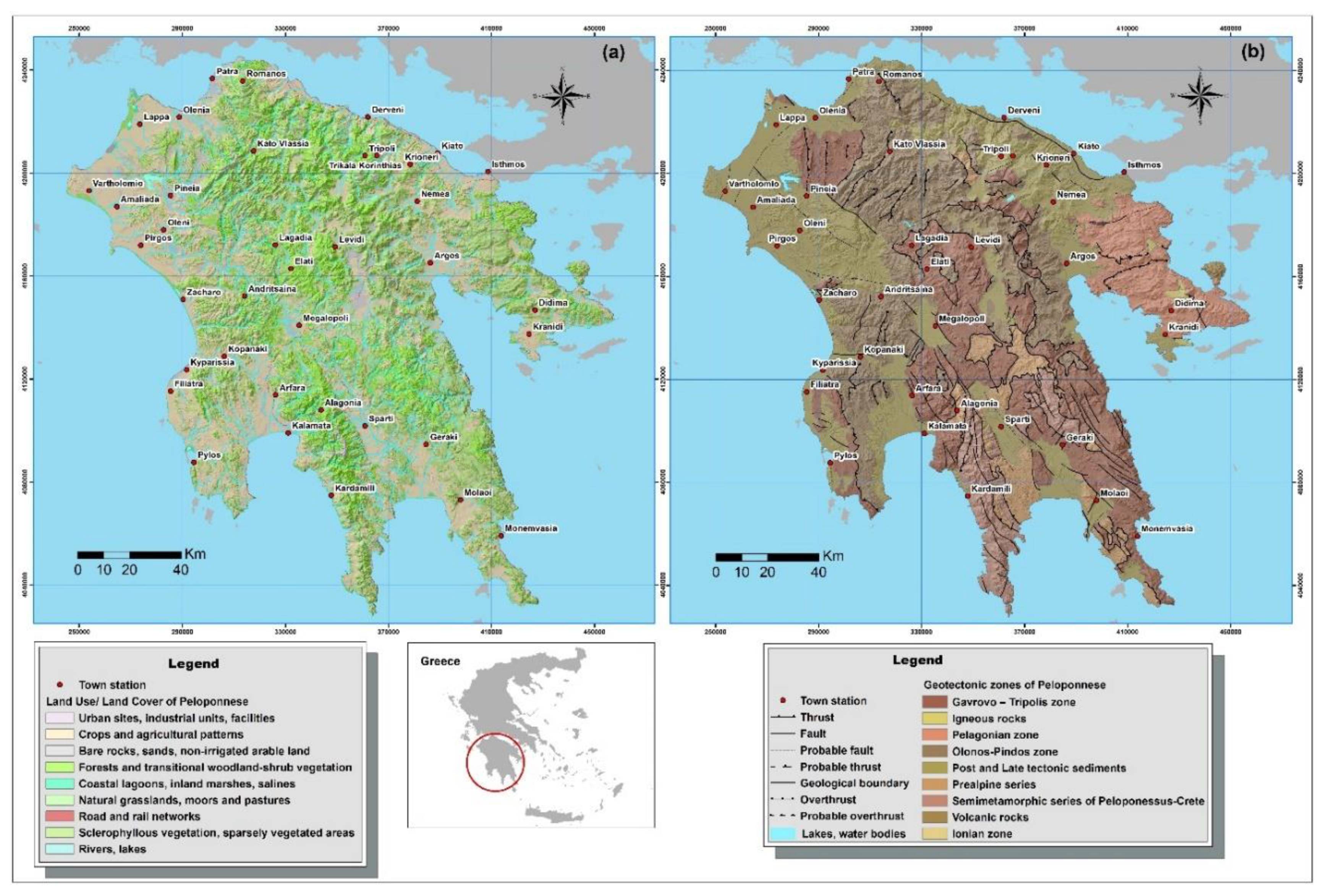
MODIS products of net ET (MOD16A2V6) have been acquired (32 images) from EarthExplorer and EARTHDATA platforms (https://earthexplorer.usgs.gov/ (accessed on 11 February 2021); https://urs.earthdata.nasa.gov/ (accessed on 11 February 2021)). Evapotranspiration MOD16A2V6 products are not raw data, but are produced based on a recently updated complex algorithm [61] based on Penman–Monteith equation, which employs reanalysis meteorological data (humidity, air temperature, radiation) from NASA’s Global Modeling and Assimilation Office (GMAO, v.4.0.0) and remote sensed vegetation data. Each one of the 32 images constitutes an 8-day composite of ET and includes, amongst other layers, net ET (cell size of 500 m). The images were then appropriately prepared in ArcMap 10.6 (reprojection, masked with the outline of the study area, cell size of 1000 to be compatible with the distributions of ETo distributions (see Section 2.2)). Then the images of each month were averaged (using cell statistics (mean) command, set to ignore no data pixels). Thus, the mean daily MODIS ET (mm) distributions of the study area for Augusts and Decembers of years 2016–2019 were produced.

MODIS ET is an estimate of actual ET, whereas the three methods produce ETo. Those parameters have different physical meanings and different responses to weather conditions (e.g., precipitation, wind speed). This study is the first part of a thorough research project investigating the agreement between several methods estimating ETo or ETa and the differences among the aforementioned estimates to MODIS ET estimates, and to pan evaporation measurements. This methodology presents novelty in the way methods are executed, via ArcMap models with an interactive character of letting users adjust properly the settings of their study area. They would be available for usage by other researchers and they are prone to creative expansion by researchers (both in python and in model builder environment), which makes them flexible and user-friendly. Another novelty is the creation of statistical models of RMSD, MB and NMB providing the areal value. Those models are developed in a way that they can compute indices by processing large images (with more than 20,000 values) cell-to-cell, instead of the time-consuming process of extracting points from the distributions in ArcMap and using external statistical software to compute the areal index in a series of steps, which demands expertise.

3. Study Area

Peloponnese is a peninsula to the south of Greece, occupying 21,439 km², which is about 1/6 of the Greek territory, separated from the mainland, with a population of 1,086,935 (census 2011; https://www.statistics.gr/el/statistics/-/publication/SAM03/2011 (accessed on 20 March 2021)). A large part is covered by high hills and mountains running NW to SE—the highest is Taygetus (2407 m, S). The wider plain (Ilia plain) lies over the west coastal part (Lappa to Kyparissia area). The biggest city is Patra at the north edge. The hydrographic network is well developed [62], though with few large rivers (e.g., Alfeios, Evrotas, Pineios). The main land use/land cover (LULC) types are agricultural patterns, forest and transitional vegetation (Figure 1a), a large part of which (Western Peloponnese) had been subjected to the most severe wildfires of Greece in 2007 [63].

Lithology, climate, and tectonic activity define the relief formation of the area (Figure 1b) [64]. The bedrock of Peloponnese consists of the formations of geotectonic zones (west to east), as follows: the Ionian zone, Gavrovo–Tripolis zone, Olonos–Pindos zone (External Hellenides) and Pelagonian zone (Internal Hellenides) (Figure 1b). The climate of Peloponnese is a Mediterranean warm temperate climate with a dry summer (Csa) [65,66]. The annual average temperature ranges from below 8 °C to 20 °C, precipitation ranges between 400 to over 2000 mm, and sunshine between 1900 and 3100 h (http://climatlas.hnms.gr/sdi/?lang=EN (accessed on 20 March 2021)). However, during the years 2016–2019, which are four out of the five of the warmest years since the pre-industrial era [31], there have been substantial departures from the average T (https://meteosearch.meteo.gr/ (accessed on 15 January 2021)).

Figure 1. (a) Land use /land cover map of Peloponnese (modified from [67]); (b) geotectonic zones of Peloponnese (digitized from [68]). Schemes follow the same formatting.

Figure 1. (a) Land use /land cover map of Peloponnese (modified from [67]); (b) geotectonic zones of Peloponnese (digitized from [68]). Schemes follow the same formatting.

4. Statistical Measures

There are specific statistical indices used in the literature for the assessment of the agreement between the different methods of ET estimation [22,47,59,60]. According to the literature, the coefficient of determination (R²) has been proven as oversensitive to extreme values and insensitive to additive and proportional differences between the compared values, thus it is characterized as a rather misleading goodness of fit for hydrological parameters [69]. For these reasons, the root-mean-square difference (RMSD), mean bias (MB) and normalized mean bias (NMB) were used, which are satisfactorily reliable [70]. The root-mean-square difference expresses the average difference between the compared values of ET (in mm). The mean bias (MB) demonstrates the bias or the mean bias error (MBE) (in mm) (Table 2). The normalized mean bias (NMB) or normalized mean bias error (NMBE) (Table 2) are both dimensionless measures, so that direct comparisons of ET values between different time scales are possible. Aiming to calculate RMSD, MB and NMB values between pairs of methods, models have been developed in ArcMap 10.6 (model builder). Those models are easy and quick to run, while they process raster images (213*218) with more than 20,000 (valid) pixels. The plots display MB and NMB rather than MBE and NMBE, respectively, since they have the same absolute value, but the former are signed. A plus sign (+) expresses the overestimation of the method compared to the reference, whereas a minus sign (−) expresses underestimation. The model of RMSD results in a raster of squared differences (RSMD²) calculated cell-to-cell and their mean value, the square root of which is RSMD. The MB model results in a raster of differences (cell-to-cell), the mean value of which represents MB. The model producing NMB masks the denominator raster, using the nominator raster as a mask in order to acquire the same size (213*218) and exactly the same no data pixels as the nominator raster.

5. Results

5.1. Descriptive Statistics (Mean, SD) of Areal Daily ETo and MODIS ET

As presented in

Table 3. Descriptive statistics of areal daily mean ETo (mm) and MODIS ET (mm) of Decembers and Augusts for years 2016–2019.

	December ETo Daily Mean (SD)				August ETo Daily Mean (SD)
	FAO PM	HS	Hansen	MODIS	FAO PM	HS	Hansen	MODIS
2016	1.37 (0.17)	0.89 (0.11)	0.98 (0.09)	0.80 (0.12)	5.30 (0.80)	4.87 (0.45)	4.30 (0.33)	1.58 (0.61)
2017	1.59 (0.31)	0.89 (0.11)	0.97 (0.08)	0.80 (0.13)	5.53 (0.49)	5.53 (0.49)	2.86 (0.16)	1.46 (0.56)
2018	1.35 (0.28)	0.92 (0.11)	1.00 (0.08)	0.88 (0.15)	5.21 (0.27)	4.61 (0.34)	4.12 (0.17)	1.93 (0.70)
2019	1.45 (0.23)	0.96 (0.10)	1.02 (0.07)	0.98 (0.17)	5.74 (0.28)	5.16 (0.38)	4.53 (0.26)	1.71 (0.66)

, the daily mean ETo estimates by FAO PM are greater, followed for December by the Hansen’s and HS’s estimates. The MODIS ET mean values are closer to the Hansen mean values. For August, FAO PM produces higher estimates followed by HS and Hansen. The MODIS ET values are substantially lower than empirical methods’ estimates, and similar to the FAO PM estimates for December (Table 3).

5.2. Daily Mean ETo Estimates for Decembers and Augusts

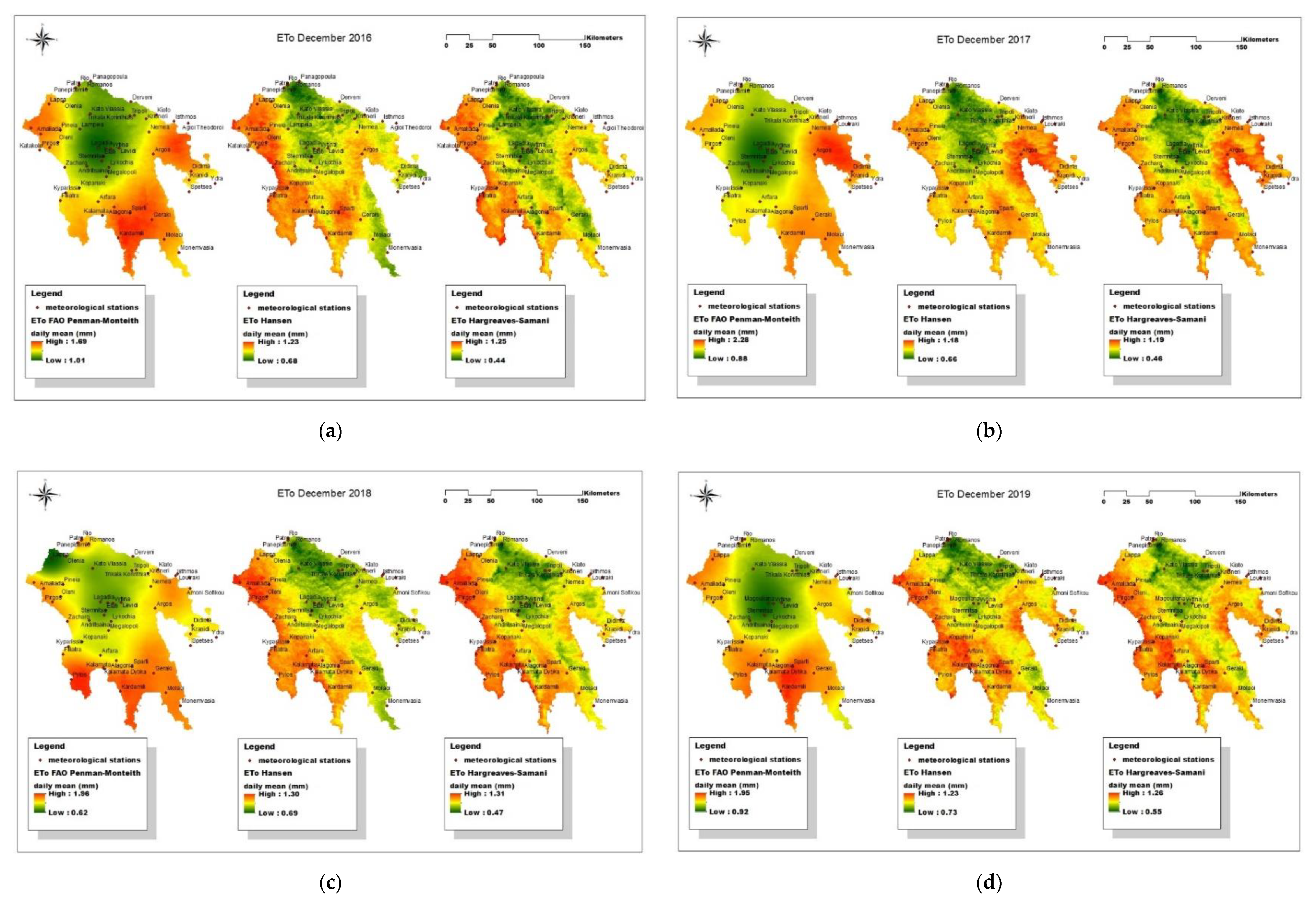
5.2.1. Spatial Distributions of Daily Mean ETo for Decembers and Augusts

The outcomes of the models for FAO PM, Hansen and HS for the December daily mean ETo of the years 2016–2019 are shown in Figure 2a–d. FAO PM produces greater values, whereas Hansen and HS appear to have a closer range of values, especially the maximum values. As depicted in Figure 3a–d, FAO PM appears to have closer estimates to HS for August, whereas Hansen produces lower ones. However, the departures of the FAO PM range for August 2019 and for the maximum value of August 2016 are noted.

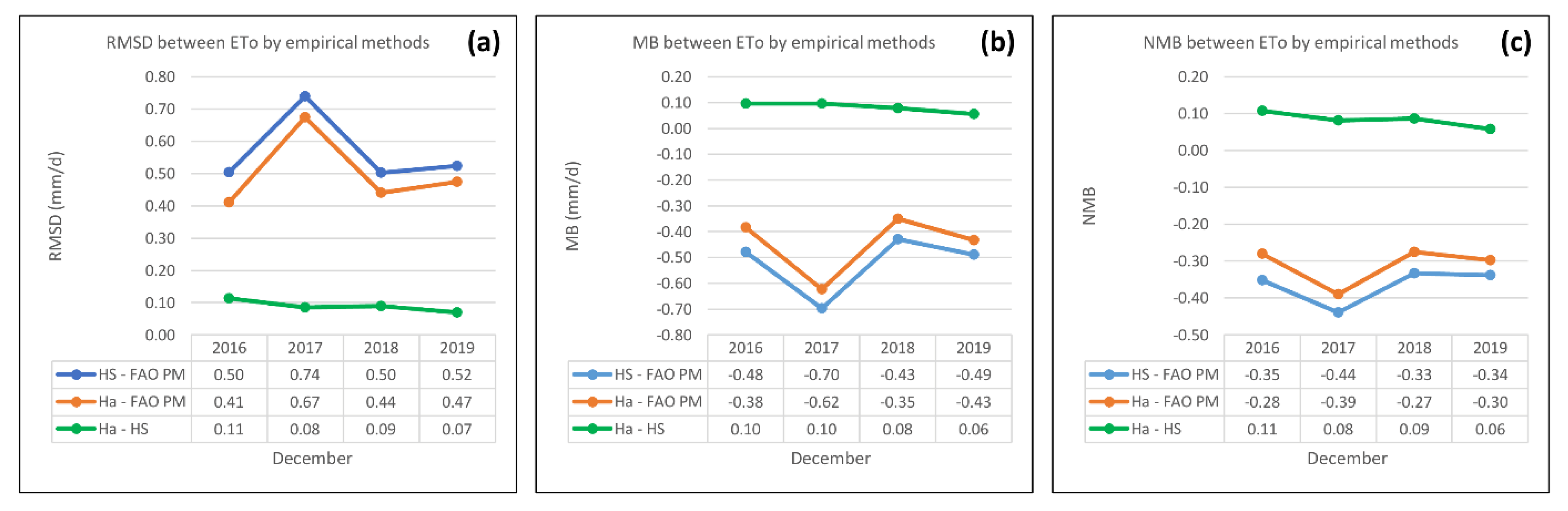
5.2.2. Statistical Measures between Estimates by Empirical Methods

It is obvious by the statistical indices (RMSD, MB and NMB) that Hansen and HS display RMSD ≤ 0.11 mm in the daily mean ETo estimation of December for the 4 years (Figure 4). Concerning the reference method (FAO PM), Hansen is closer with the latter underestimating ETo (RMSD between 0.41 and 0.67 mm d⁻¹), whereas the corresponding RMSD for HS lies within 0.50–0.74 mm d⁻¹, with the maximum daily mean ETo appearing for December 2017. For August, the statistical indices indicate that the HS and FAO PM estimates are consistently close, with the former underestimating ETo with an RMSD between 0.72 and 0.76 mm d⁻¹ (Figure 5). It is obvious that for August 2017 the estimation by Hansen shows significant departure, thus explaining the differentiation between Hansen and HS, which generally display close estimations (RMSD ≤ 0.66 mm d⁻¹) for the Augusts (slight underestimation by Hansen) of the other 3 years.

5.3. Daily Mean MODIS ET Estimates for Decembers and Augusts

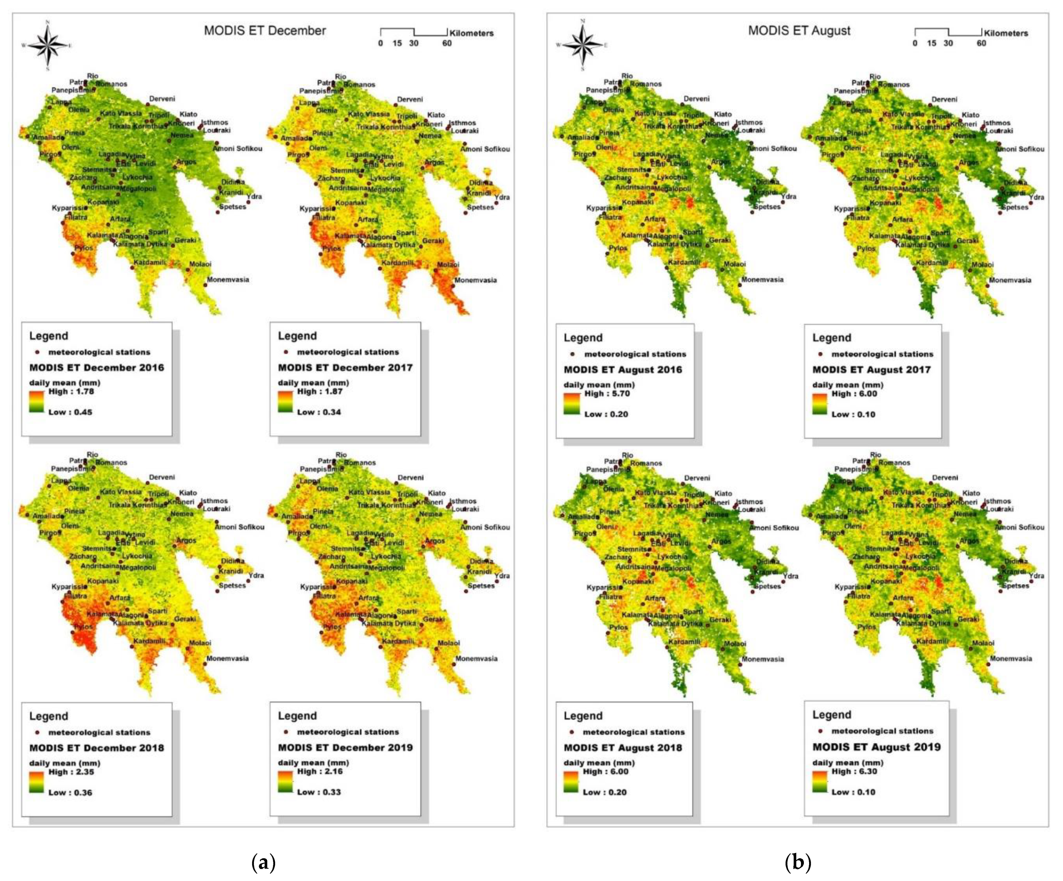
5.3.1. Spatial Distributions of Daily Mean MODIS ET for Decembers and Augusts

As shown in Figure 6a, the daily mean values of the December MODIS ETs for 2018 and 2019 exhibit greater maximum values, whereas the minimum values are similar (0.33–0.36 mm), except from 2016, which is slightly higher (0.45 mm). As Figure 6b demonstrates, there is a gradual increase in the maximum daily mean values of MODIS ET from 2016 to 2019, whereas the minimum values are either 0.10 mm (2017, 2019) or 0.20 mm (2016, 2018).

5.3.2. Statistical Measures for Investigating the Difference between Empirical ETo and MODIS ET Estimates for Decembers and Augusts

As shown in Figure 7, HS and MOD16A2V6 produce very close estimations for the daily mean ET in December for all of the years (RMSD between 0.15 and 0.17 mm d⁻¹), with the former appearing to have higher values. Hansen follows with higher values compared against MOD16A2V6, ranging between 0.16 and 0.22 mm d¹. FAO PM shows the greatest difference to MOD16A2V6 (RMSD around 0.62 mm d⁻¹ on average for the 4 years), with a maximum deviation for RMSD in December 2017 (0.84 mm d⁻¹). Figure 8 depicts that the deviations between the empirical methods and MOD16A2V6 are considerable for the August daily mean values, with the latter appearing to have substantially lower daily mean values compared to FAO PM. Hansen is closer to the MOD16A2V6 estimation, with the latter appearing to have lower ET values (RMSD between 1.51 and 2.91 mm d⁻¹). Moreover, the minimum disagreement between the Hansen and MODIS estimations was found for August 2017. The latter, along with the largest deviation for August 2017 by Hansen against the rest empirical methods (Figure 8) underlined above, implies that the Hansen and MODIS algorithms may share sensitivity (or degrees of freedom). Compared to MODIS, HS exhibits an RMSD between 2.80 and 3.68 mm d⁻¹, and FAO PM an RMSD between 3.36 and 4.13 mm d⁻¹. The fact that the empirical methods produced greater values compared to MODIS is shown by the positive signs of the MB and NMB indices.

6. Discussion

6.1. Parameters Differentiating the Distributions of Reference Evapotranspiration (ETo) and MODIS ET

For December 2016 (see Figure 2a), although all of the methods assign the lowest values to the northcentral part the physically based FAO PM differentiated from HS and Hansen by assigning the maximum values in the following two patterns: where the maximum u₂ (>12.50 ms⁻¹) and elevated Rn occurs (eastern part), or when the maximum Rn (>2.53 MJ m⁻²) and elevated u₂ (>7.30 ms⁻¹) is encountered (SE part). For December 2017 (see Figure 2b), Hansen and HS demonstrate almost identical distributions. FAO PM differentiates the northcentral edge due to a very high mean monthly u₂ (>9.50 ms⁻¹). The sensitivity of FAO PM towards u₂ and Rn is responsible for a maximum of 1 mm greater than those of the rest methods assigned to the area around Argos, where VPD is the maximum (0.48 kPa) (u₂: 7.99–13.46 ms⁻¹, Rn: 2.56–2.63 MJ m⁻² and VPD: 0.30–0.35 kPa). For December 2018 (see Figure 2c), Hansen and HS exhibit similar contributions and a similar range of values. The main difference is the green area, which FAO PM assigns at the northwestern part, which is due to the very low monthly mean u₂ reported at the station (<0.09 ms⁻¹) since the other parameters are rather elevated (VPD = 0.38 kPa and Rn = 2.17 MJ m⁻²), expressing the sensitivity of FAO PM to wind speed (u₂) not only for the maximum, but also for the minimum ETo values assignments. For December 2019 (see Figure 2d), FAO PM displays the maximum due to increased Rn (>2.61 MJ m⁻²) and u₂ (>7.78 ms⁻¹). The high u₂ (>9.65 ms⁻¹) at the northcentral edge is responsible for the yellow color in the FAO PM distribution in contradiction with the green color assigned by the other methods that do not incorporate u₂.

For August 2016 (see Figure 3a) FAO PM by the green central zone reflects that Rn and u2 are both low, and VPD is elevated. The eastern part of Peloponnese displays similarity for all of the methods with a maximum where the monthly mean values of T and Rn, wind speed and VPD are the maximum of Peloponnese. For August 2017 (see Figure 3b), FAO PM contribution resembles that of 2016; however, the rest of the methods display differentiated distributions with enough similarities to each other. The maximum values of FAO PM are displayed over the south-central spots where both Rn and u₂ have some of the greatest monthly mean values reported, followed by the values over the western part. The latter is also displayed by both the Hansen and HS methods. Kardamili and Molai exhibit lower values of Rs (depicted by the green color of Hansen and HS), but also increased values of u₂, reflected only in FAO PM (yellow color). The obvious difference over the central part, which is green in FAO PM but redish in the other methods’ distributions, is that those stations display increased Rs (and Rn) values in which the three methods are sensitive, but also elevated VPD values (around 1.0 kPa) and low u₂ values. FAO PM is the only method incorporating all of those parameters. The northcentral part exhibits low values for all of the parameters.

For August 2018 (see Figure 3c), the Hansen and HS distributions look almost identical, even if Hansen’s maximum value is a little lower. The maximum ET values for the three methods are displayed over the west part, the same as in 2017 (increased Rn, u₂ and VPD values). FAO PM assigns the west-central spots to the yellow scale, recognizing the lower u₂ values (average <1.40 ms⁻¹). The eastern part and SC spots display high values due to the elevated values of the pattern Rn and u2 (similar VPD values). The FAO PM distribution reflects the same general pattern as in 2016 and 2017, with the green zone trending from the north-central to the southwestern part; however, with the zones of lower values merely declined. Moreover, even if FAO PM has a central green zone, the fact that its minimum (green) value (4.56 mm) corresponds to the medium (yellow–orange) values of the other two methods practically assigns similar ET values to the central part. The green areas of the Hansen and HS methods have all in common low Rs values. HS assigns the S part to the yellow scale, which is closer to the FAO PM output. The latter appears to have a minimum value of 1 mm greater probably because of the u₂ elevated values [71]. For August 2019 (see Figure 3d), the maximum values of FAO PM and HS are around 6.30 mm. FAO PM assigns the highest values to the northeastern part (Rn and u₂ pattern). FAO PM has a diminished green zone compared to the previous years around the central mountainous part, turning into yellow as the values of Rn and u2 increase. Hansen and HS assign high values only around Sparti station, which has the highest Rs, neglecting the increased u2 values (around 8.00 ms⁻¹) of the nearby stations.

Throughout the years, August 2016 exhibits higher maximum values at the southmost part (around Geraki). Regarding the distribution by FAO PM, it is obvious that the green central lane from the northmost to southmost edges in 2016 is eventually diminished to just the central mountainous part in 2019. This spreading of the redish areas with the years can also be noticed from the distributions of the other two methods with a lower consistency over the years. Our findings are in line with the seasonality, which makes empirical methods deviate more during the summertime, as several researchers have noted not only for the South Mediterranean areas in general, but also specifically for Greece [47]. Both Hansen and HS exhibit good performance (low RMSD) in the winter season, but poor performance in the summer season. Their performance has been reported to be the opposite for the winter and summer of neighboring areas with humid climates (e.g., Serbia [55])

6.2. Differences and Similarities between Estimates of Reference Evapotranspiration (ETo) and MODIS ET

MODIS ET is a product of a sophisticated algorithm; however, it produces considerable underestimation in the literature (such as by 26%; [72]; and by 25% uncertainty [73]) compared with sites of the AmeriFlux network, which has been used for the calibration of the updated algorithm [61] attributed to the need of further refinement. Besides, global satellite products generally contain more noise than ground-based measurements lacking in accuracy [33,74]. Westerhoff (2015) [74] has conservatively set the uncertainty of satellite to ground-based estimations equal to 1.5. For December, FAO PM showed the greatest difference to MOD16A2V6 for all of the statistical indices (e.g., RMSD: 0.52–0.84 mm d⁻¹, MB: 0.47–0.78 mm d⁻¹). HS appeared to have a minimal difference to MODIS ET (e.g., RMSD: 0.15–0.17 mm d⁻¹, MB: –0.02–0.09 mm d⁻¹) and Hansen followed (RMSD: 0.16–0.22 mm d⁻¹, MB: 0.03–0.18 mm d⁻¹). Moreover, all of the empirical methods compared to MODIS ET, except from Hansen, exhibited the greatest departures (maximums) in statistical indices (demonstrating lowest agreement) for 2017. Relative studies in Greece report accuracy of empirical methods’ performances during the winter. Aiming at investigating whether good performance is a seasonal characteristic also for 2016–2019, the research should be expanded to the rest of the months of this period. The estimates of ETo are close to MODIS ET in the Decembers of 2016–2019, because although the former reflects the evaporative demand of the atmosphere, the latter is an estimate of actual ET subjected to water stress. However, during December the evaporative demand of the atmosphere is low, the VPD is low (thus relative humidity is elevated), and December is the month with the third highest precipitation (in mm) in Greece, so the evaporative demand is satisfied.

The opposite happens during the Augusts when the evaporative demand is elevated (high Rn, T, VPD and low u₂), but due to water stress during the summertime it cannot be adequately satisfied. Thus, the MODIS ET values are considerably lower than the ETo estimates, with the former appearing values almost at the levels of December (i.e., FAO PM values for December). FAO PM differs the most from MODIS (as also in December) (RMSD: 3.87–4.06 mm d⁻¹, MB: 3.26–4.06 mm d⁻¹) due to its incorporation of more climate parameters, and the Hansen estimates are the closest to the MODIS ones (RMSD: 1.51–2.91 mm d⁻¹, MB: 0.96–1.71 mm d⁻¹) followed by HS; however, with considerable discrepancies in both cases. The Hansen ETo values exhibit the greatest difference from the MODIS actual ET estimates for the two warmest years (2016 and 2019). Considering the physical meaning of ETo and MODIS ET, this might imply Hansen being more affected by Rs (and subsequently by T) than the rest. Another observation is that Hansen bears similar departures in the estimates to MODIS ET for August 2017, which should be further investigated in terms of sensitivity.

The main limitations are the following: Rs is not measured during the study years but computed under the FAO guidelines for missing data, with a KT (0.17) coefficient used for both coastal and mainland areas. Moreover, the constant value (0.23) used for albedo, the replacement of which is with MODIS albedo products, would refine the estimates. Model builder in ArcMap cannot process raster images and point features together, thus the RMSD model bears the limitation of producing the squared areal RMSD value (RMSD²). However, the square root of a number can be trivially computed.

The primary contribution of the study is that the application of ETo models and statistical models addresses international and interdisciplinary interest. Moreover, the produced maps of ETo and MODIS ET of Peloponnese can be used for comparisons against the local ETo and ETa estimates produced by other methods or from data acquired from alternative sources. In particular, FAO PM distributions could be employed as a reference by researchers. Moreover, considering their physical meaning, ETo and MODIS ET maps of the most warm recent years provide water managers of Peloponnese with a general picture, which can be integrated to define the irrigation needs during the Augusts [34,51], and the flooding risks during the Decembers [50].

7. Conclusions

Our findings are in line with the seasonality, which makes the empirical methods more accurate in the winter (December) and deviate more during the summertime (August), both for the South Mediterranean areas and specifically for Greece. For the Decembers of 2016–2019, the estimates by HS and Hansen are almost identical (NMB up to 0.11 mm), but FAO PM produces higher estimates attributed to the wind speed (u₂) sensitivity of the latter. For August 2016–2019, HS and FAO PM present almost identical estimates, probably because the wind speed values can be neglected for the majority of the cells. The Hansen method produces departures (lower values) for August 2017 compared to the rest. These departures are also observed for MODIS ET, thus the relations would be investigated in terms of physical or computational factors, which affect alike the sensitivity of the two different approaches.

The areal daily mean MODIS ET, as an estimate of the actual ET, was examined along with the methods’ ETo estimates. Since they have different physical meanings, the ETo values for the Augusts 2016–2019 were much higher than MODIS anticipated. However, for the Decembers 2016–2019, HS produced almost identical estimates (NMB between −0.02 and 0.11) with the MODIS ET averaged products. This is attributed to the low evaporative demand during December, which can be satisfied by rainfall. HS could be used satisfactorily regarding the accuracy for the estimation of the daily mean actual ET of Peloponnese for the Decembers 2016–2019. The latter could be further investigated for a larger period of years for the rest of the winter months.

Partitioning Peloponnese into rough segments with similar climate characteristics and LULC, in order to calibrate the empirical methods for the local and regional spatial scales for the monthly time scale, is proposed for future research, since it could assess the performance of empirical methods during different seasons and LULC types. Moreover, examination of ETo along with ETa, MODIS ET and Epan would contribute to the perception of their complex relations despite their substantial differences.

References

1. Long, D.; Longuevergne, L.; Scanlon, B.R. Uncertainty in evapotranspiration from land surface modeling, remote sensing, and GRACE satellites. Water Resour. Res. 2014, 50, 1131–1151. [Google Scholar] [CrossRef] [Green Version]
2. Xu, S.; Yu, Z.; Yang, C.; Ji, X.; Zhang, K. Trends in evapotranspiration and their responses to climate change and vegetation greening over the upper reaches of the Yellow River Basin. Agric. For. Meteorol. 2018, 263, 118–129. [Google Scholar] [CrossRef]
3. Liu, Z.; Ballantyne, A.P.; Cooper, L.A. Biophysical feedback of global forest fires on surface temperature. Nat. Commun. 2019, 10. [Google Scholar] [CrossRef] [Green Version]
4. Sidiropoulos, P.; Dalezios, N.R.; Loukas, A.; Mylopoulos, N.; Spiliotopoulos, M.; Faraslis, I.N.; Alpanakis, N.; Sakellariou, S. Quantitative Classification of Desertification Severity for Degraded Aquifer Based on Remotely Sensed Drought Assessment. Hydrology 2021, 8, 47. [Google Scholar] [CrossRef]
5. Tigkas, D.; Vangelis, H.; Tsakiris, G. Implementing Crop Evapotranspiration in RDI for Farm-Level Drought Evaluation and Adaptation under Climate Change Conditions. Water Resour Manag. 2020, 34, 4329–4343. [Google Scholar] [CrossRef]
6. Vangelis, H.; Tigkas, D.; Tsakiris, G. The effect of PET method on Reconnaissance Drought Index (RDI) calculation. J. Arid Environ. 2013, 88, 130–140. [Google Scholar] [CrossRef]
7. Mosavi, A.; Edalatifar, M. A Hybrid Neuro-Fuzzy Algorithm for Prediction of Reference Evapotranspiration. In Recent Advances in Technology Research and Education. INTER-ACADEMIA 2018. Lecture Notes in Networks and Systems; Laukaitis, G., Ed.; Springer: Cham, Switzerland, 2019; Volume 53. [Google Scholar] [CrossRef]
8. Sattari, M.T.; Apaydin, H.; Band, S.S.; Mosavi, A.; Prasad, R. Comparative analysis of kernel-based versus ANN and deep learning methods in monthly reference evapotranspiration estimation. Hydrol. Earth Syst. Sci. 2021, 25, 603–618. [Google Scholar] [CrossRef]
9. Shamshirband, S.; Hashemi, S.; Salimi, H.; Samadianfard, S.; Asadi, E.; Shadkani, S.; Kargar, K.; Mosavi, A.; Nabipour, N.; Chau, K.W. Predicting Standardized Streamflow index for hydrological drought using machine learning models. Eng. Appl. Comput. Fluid Mech. 2020, 14, 339–350. [Google Scholar] [CrossRef]
10. Andreu, A.; Kustas, W.P.; Polo, M.J.; Carrara, A.; González-Dugo, M.P. Modeling Surface Energy Fluxes over a Dehesa (Oak Savanna) Ecosystem Using a Thermal Based Two Source Energy Balance Model (TSEB) II—Integration of Remote Sensing Medium and Low Spatial Resolution Satellite Images. Remote Sens. 2018, 10, 558. [Google Scholar] [CrossRef] [Green Version]
11. Silva, A.M.; da Silva, R.M.; Santos, C.A.G. Automated surface energy balance algorithm for land (ASEBAL) based on automating endmember pixel selection for evapotranspiration calculation in MODIS orbital images. Int. J. Appl. Earth Obs. Geoinf. 2019, 79, 1–11. [Google Scholar] [CrossRef]
12. Mutiibwa, D.; Strachan, S.; Albright, T. Land Surface Temperature and Surface Air Temperature in Complex Terrain. IEEE J. Sel. Top. Appl. Earth Obs. Remote Sens. 2015, 8, 4762–4774. [Google Scholar] [CrossRef]
13. Jin, M.; Dickinson, R.E. Land Surface Skin Temperature Climatology: Benefitting from the Strengths of Satellite Observations. Environ. Res. Lett. 2010, 5, 044004. [Google Scholar] [CrossRef] [Green Version]
14. Wan, Z. New refinements and validation of the MODIS land-surface temperature/emissivity products. Remote Sens. Environ. 2008, 112, 59–74. [Google Scholar] [CrossRef]
15. Raoufi, R.; Beighley, E. Estimating Daily Global Evapotranspiration Using Penman–Monteith Equation and Remotely Sensed Land Surface Temperature. Remote Sens. 2017, 9, 1138. [Google Scholar] [CrossRef] [Green Version]
16. Lin, S.; Moore, N.J.; Messina, J.P.; DeVisser, M.H.; Wu, J. Evaluation of estimating daily maximum and minimum air temperature with MODIS data in east Africa. Int. J. Appl. Earth Obs. Geoinf. 2012, 18, 128–140. [Google Scholar] [CrossRef]
17. Kitsara, G.; Papaioannou, G.; Retalis, A.; Paronis, D.; Kerkides, P. Estimation of air temperature and reference evapotranspiration using MODIS land surface temperature over Greece evapotranspiration using MODIS land surface temperature. Int. J. Remote Sens. 2018, 39, 924–948. [Google Scholar] [CrossRef]
18. Trepekli, A.; Loupa, G.; Rapsomanikis, S. Agricultural and Forest Meteorology Seasonal evapotranspiration, energy fluxes and turbulence variance characteristics of a Mediterranean coastal grassland. Agric. For. Meteorol. 2016, 226–227, 13–27. [Google Scholar] [CrossRef]
19. Vancutsem, C.; Ceccato, P.; Dinku, T.; Connor, S.; Lin, J. Evaluation of MODIS land surface temperature data to estimate air temperature in different ecosystems over Africa. Remote Sens. Environ. 2010, 114, 449–465. [Google Scholar] [CrossRef]
20. Zhu, W.; Lu, A.; Jia, S. Estimation of daily maximum and minimum air temperature using MODIS land surface temperature products. Remote Sens. Environ. 2013, 130, 62–73. [Google Scholar] [CrossRef]
21. Allen, R.; Pereira, L.; Raes, D.; Smith, M. Crop evapotranspiration–Guidelines for computing crop water requirements. In Irrigation and Drainage, Paper No. 56; FAO: Rome, Italy, 1998; p. 300. Available online: http://www.fao.org/3/x0490e/x0490e07.htm#estimating%20missing%20climatic%20data (accessed on 21 April 2021).
22. Dalezios, N.R.; Loukas, A.; Bampzelis, D. Spatial variability of reference evapotranspiration in Greece. Phys. Chem. Earth 2002, 27, 1031–1038. [Google Scholar] [CrossRef]
23. Xu, Y.; Knudby, A.; Ho, H.C. Estimating daily maximum air temperature from MODIS in British Columbia, Canada. Int. J. Remote Sens. 2014, 35, 8108–8121. [Google Scholar] [CrossRef]
24. Vicente-Serrano, S.M.; Saz-Sánchez, M.A.; Cuadrat, J.M. Comparative analysis of interpolation methods in the middle Ebro Valley (Spain): Application to annual precipitation and temperature. Clim. Res. 2003, 24, 161–180. [Google Scholar] [CrossRef] [Green Version]
25. Chatzithomas, C.D.; Alexandris, S.G. Solar radiation and relative humidity based, empirical method, to estimate hourly reference evapotranspiration. Agric. Water Manag. 2015, 152, 188–197. [Google Scholar] [CrossRef]
26. Allen, R.G.; Walter, I.A.; Elliot, R.; Howell, T.; Itenfisu, D.; Jensen, M. The ASCE standardized reference evapotranspiration equation. Final report. In National Irrigation Symp; ASCE-EWRI: Phoenix, AZ, USA, 2005. [Google Scholar]
27. Pereira, L.S.; Allen, R.G.; Smith, M.; Raes, D. Crop evapotranspiration estimation with FAO 56: Past and future. Agric. Water Manag. 2015, 147, 4–20. [Google Scholar] [CrossRef]
28. Dimitriadou, S.; Nikolakopoulos, K.G. Remote sensing methods to estimate evapotranspiration incorporating MODIS derived data and applications over Greece: A review. In Proceedings of the SPIE 11524, Eighth International Conference on Remote Sensing and Geoinformation of the Environment (RSCy2020), Paphos, Cyprus, 26 August 2020; p. 1152405. [Google Scholar] [CrossRef]
29. Proias, G.; Gravalos, I.; Papageorgiou, E.; Poczęta, K.; Sakellariou-Makrantonaki, M. Forecasting Reference Evapotranspiration Using Time Lagged Recurrent Neural Network. Wseas Trans. Environ. Dev. 2020, 16, 699–707. [Google Scholar] [CrossRef]
30. Loukas, A.; Vasiliades, L.; Domenikiotis, C.; Dalezios, N.R. Basin-wide actual evapotranspiration estimation using 3 NOAA/AVHRR satellite data. Phys. Chem. EarthParts A/B/C 2004, 30, 69–79. [Google Scholar] [CrossRef]
31. Loukas, A.; Vasiliades, L.; Domenikiotis, C.; Dalezios, N.R. Water balance of forested mountainous watersheds using satellite-derived actual evapotranspiration. In Proceedings of the SPIE 5232, Remote Sensing for Agriculture, Ecosystems, and Hydrology V, Barcelona, Spain, 24 February 2004. [Google Scholar] [CrossRef]
32. Gourgoulios, V.; Nalbantis, I. Ungauged drainage basins: Investigation on the basin of Peneios River, Thessaly, Greece. Eur. Water 2017, 57, 163–169. [Google Scholar]
33. Toulios, L.; Spiliotopoulos, M.; Papadavid, G.; Loukas, A. Observation Methods and Model Approaches for Estimating Regional Crop Evapotranspiration and Yield in Agro-Landscapes: A Literature Review. In Landscape Modelling and Decision Support. Innovations in Landscape Research; Mirschel, W., Terleev, V., Wenkel, K.O., Eds.; Springer: Cham, Switzerland, 2013; pp. 79–100. ISBN 978-3-030-37420-4. [Google Scholar] [CrossRef]
34. Malamos, N.; Tsirogiannis, I.L.; Tegos, A.; Efstratiadis, A.; Koutsoyiannis, D. Spatial interpolation of potential evapotranspiration for precision irrigation purposes. Eur. Water 2017, 59, 303–309. [Google Scholar]
35. Nastos, P.; Kapsomenakis, J.; Kotsopoulos, S.; Poulos, S. Present and future projected reference evapotranspiration over Thessaly plain, Greece, based on regional climate models’ simulations. Eur. Water 2015, 51, 63–72. [Google Scholar]
36. Sakellariou-Makrantonaki, M.; Vagenas, I.N. Mapping crop evapotranspiration and total crop water requirements estimation in central Greece. Eur. Water 2006, 13–14, 3–13. [Google Scholar]
37. Gudulas, K.; Voudouris, K.; Soulios, G.; Dimopoulos, G. Comparison of different methods to estimate actual evapotranspiration and hydrologic balance. Desalination Water Treat. 2013, 51, 2945–2954. [Google Scholar] [CrossRef]
38. Voudouris, K.S.; Georgiou, P.E.; Mavromatis, T.; Gianneli, C. Comparison of actual evapotranspiration estimation methods: Application to Korisos basin, NW Greece. In Evapotranspiration: Processes, Sources and Environmental Implications, 1st ed.; Er-Raki, S., Ed.; Nova Sciences Publishers: New York, NY, USA, 2013; pp. 105–118. ISBN 978-1-62417-138-3. [Google Scholar]
39. Aschonitis, V.; Miliaresis, G.; Demertzi, K.; Papamichail, D. Terrain Segmentation of Greece Using the Spatial and Seasonal Variation of Reference Crop Evapotranspiration. Adv. Meteorol. 2016, 2016, 3092671. [Google Scholar] [CrossRef] [Green Version]
40. Demertzi, K.; Pisinaras, V.; Lekakis, E.; Tziritis, E.; Babakos, K.; Aschonitis, V. Assessing Annual Actual Evapotranspiration based on Climate, Topography and Soil in Natural and Agricultural Ecosystems. Climate 2021, 9, 20. [Google Scholar] [CrossRef]
41. Spiliotopoulos, M.; Adaktylou, N.; Loukas, A.; Michalopoulou, H.; Mylopoulos, N.; Toulios, L. A spatial downscaling procedure of MODIS derived actual evapotranspiration using Landsat images at central Greece. In Proceedings of the SPIE 8795, First International Conference on Remote Sensing and Geoinformation of the Environment (RSCy2013), Paphos, Cyprus, 5 August 2013; p. 879508. [Google Scholar] [CrossRef]
42. Falalakis, G.; Gemitzi, A. A simple method for water balance estimation based on the empirical method and remotely sensed evapotranspiration estimates. J. Hydroinform. 2020, 22, 440–451. [Google Scholar] [CrossRef]
43. Tsouni, A.; Kontoes, C.; Koutsoyiannis, D.; Elias, P. Estimation of Actual Evapotranspiration by Remote Sensing. Sensors 2008, 8, 3586–3600. [Google Scholar] [CrossRef] [PubMed]
44. Vasiliades, L.; Spiliotopoulos, M.; Tzabiras, J.; Loukas, A.; Mylopoulos, N. Estimation of crop water requirements using remote sensing for operational water resources management. In Proceedings of the SPIE 9535, Third International Conference on Remote Sensing and Geoinformation of the Environment (RSCy2015), Paphos, Cyprus, 19 June 2015; p. 95351. [Google Scholar] [CrossRef]
45. Paparrizos, S.; Maris, F.; Matzarakis, A. Sensitivity analysis and comparison of various potential evapotranspiration formulae for selected Greek areas with different climate conditions. Appl. Clim. 2017, 128, 745–759. [Google Scholar] [CrossRef]
46. Mamassis, N.; Panagoulia, D.; Novkovic, A. Sensitivity analysis of Penman evaporation method. Glob. Nest J. 2014, 16, 628–639. [Google Scholar]
47. Efthimiou, N.; Alexandris, S.; Karavitis, C.; Mamassis, N. Comparative analysis of reference evapotranspiration estimation between various methods and the FAO56 Penman—Monteith procedure. Eur. J. Water Qual. 2013, 42, 19–34. [Google Scholar]
48. Diamantopoulou, M.J.; Georgiou, P.E.; Papamichail, D.M. Performance evaluation of artificial neural networks in estimating reference evapotranspiration with minimal meteorological data. Glob. Nest J. 2011, 13, 18–27. [Google Scholar]
49. World Meteorological Organization (WMO). WMO Confirms 2019 as Second Hottest Year on Record. 15 January 2020. Available online: https://public.wmo.int/en/media/press-release/wmo-confirms-2019-second-hottest-year-record (accessed on 1 March 2021).
50. Mimikou, M.; Baltas, E. Assessment of Climate Change Impacts in Greece: A General Overview. Am. J. Clim. Chang. 2013, 2, 46–56. [Google Scholar] [CrossRef]
51. Kotsopoulos, S.I.; Nastos, P.; Lazogiannis, K.; Poulos, S.; Ghionis, G.; Alexiou, I.; Panagopoulos, A.; Farsirotou, E.; Alamanis, N. Evaporation, Evapotranspiration and crop water requirements under present and future climate conditions at Pinios delta plain. In Proceedings of the 14th International Conference on Environmental Science and Technology (CEST), Rhodes, Greece, 3–5 September 2015. [Google Scholar]
52. Varotsos, K.V.; Karali, A.; Lemesios, G.; Kitsara, G.; Moriondo, M.; Dibari, C.; Leolini, L.; Giannakopoulos, C. Near future climate change projections with implications for the agricultural sector of three major Mediterranean islands. Reg. Environ. Chang. 2021, 21, 1–15. [Google Scholar] [CrossRef]
53. Hansen, S. Estimation of potential and actual evapotranspiration. Nord. Hydrol. 1984, 15, 205–212. [Google Scholar] [CrossRef]
54. Hargreaves, G.H.; Samani, Z.A. Reference crop evapotranspiration from temperature. Appl. Eng. Agric. 1985, 1, 96–99. [Google Scholar] [CrossRef]
55. Alexandris, S.G.; Stricevic, R.J.; Petkovic, S. Comparative analysis of reference evapotranspiration from the surface of rainfed grass in central Serbia, calculated by six empirical methods against the Penman-Monteith formula. Eur. Water 2008, 21/22, 17–28. [Google Scholar]
56. Xystrakis, F.; Matzarakis, A. Evaluation of 13 Empirical Reference Potential Evapotranspiration Equations on the Island of Crete in Southern Greece. J. Irrig. Drain. Eng. 2011, 137, 211–222. [Google Scholar] [CrossRef] [Green Version]
57. Hargreaves, G.H.; Allen, R.G. History and Evaluation of Hargreaves Evapotranspiration Equation. J. Irrig. Drain. Eng. 2003, 129, 53–63. [Google Scholar] [CrossRef]
58. Samani, Z. Estimating solar radiation and evapotranspiration using minimum climatological data. J. Irrig. Drain. Eng. 2000, 126, 265–267. [Google Scholar] [CrossRef]
59. Kang, D.; Mathur, R.; Rao, S.T.; Yu, S. Bias adjustment techniques for improving ozone air quality forecasts. J. Geophys. Res. 2008, 113, D23308. [Google Scholar] [CrossRef] [Green Version]
60. Tellen, V.A. A comparative analysis of reference evapotranspiration from the surface of rainfed grass in Yaounde, calculated by six empirical methods against the penman monteith formula. Earth Perspect. 2017, 4, 4. [Google Scholar] [CrossRef] [Green Version]
61. Mu, Q.; Zhao, M.; Running, S.W. Improvements to a MODIS global terrestrial evapotranspiration algorithm. Remote Sens. Environ. 2011, 115, 1781–1800. [Google Scholar] [CrossRef]
62. Dimitriadou, S.; Katsanou, K.; Stratikopoulos, K.; Lambrakis, N. Investigation of the chemical processes controlling the groundwater quality of Ilia Prefecture. Environ. Earth Sci. 2019, 78, 401. [Google Scholar] [CrossRef]
63. Dimitriadou, S.; Katsanou, K.; Charalabopoulos, S.; Lambrakis, N. Interpretation of the Factors Defining Groundwater Quality of the Site Subjected to the Wildfire of 2007 in Ilia Prefecture, South-Western Greece. Geosciences 2018, 8, 108. [Google Scholar] [CrossRef] [Green Version]
64. Koukouvelas, I.; Mpresiakas, A.; Sokos, E.; Doutsos, T. The tectonic setting and earthquake ground hazards of the 1993 Pyrgos earthquake, Peloponnese, Greece. J. Geol. Soc. Lond. 1996, 152, 39–49. [Google Scholar] [CrossRef]
65. Argiriou, A.A. The climate of Greece; Hellenic National Meteorological Service: Athens, Greece; pp. 1–6. Available online: http://climatlas.hnms.gr/sdi/?lang=EN (accessed on 28 March 2021).
66. Kottek, M.; Grieser, J.; Beck, C.; Rudolf, B.; Rubel, F. World Map of the Köppen-Geiger climate classification updated. Meteorol. Z. 2006, 15, 259–263. [Google Scholar] [CrossRef]
67. Copernicus Land Monitoring Service. CLC 2018. © European Union, Copernicus Land Monitoring Service 2018, European Environment Agency (EEA). Available online: https://land.copernicus.eu/pan-european/corine-land-cover/clc2018 (accessed on 11 January 2021).
68. Mataragkas, D.; Triantafillou, E. Geological Map of Greece in Scale 1:1000000; Institute of Geological and Mineralogical Exploration (IGME): Athens, Greece, 1999. [Google Scholar]
69. Legates, D.R.; McCabe, G.J. Evaluating the use of “goodness–of–fit” measures in hydrologic and hydroclimatic model validation. Water Resour. Res. 1999, 35, 233–241. [Google Scholar] [CrossRef]
70. Fox, D.G. Judging air quality model performance. A summary of the AMS workshop on Dispersion Model Performance. Bull. Am. Meteorol. 1981, 62, 599–609. [Google Scholar] [CrossRef] [Green Version]
71. Raziei, T.; Pereira, L.S. Estimation of ETo with Hargreaves–Samani and FAO-PM temperature methods for a wide range of climates in Iran. Agric. Water Manag. 2013, 121, 1–18. [Google Scholar] [CrossRef]
72. Bhattarai, N.; Mallick, K.; Brunsell, N.A.; Sun, G.; Jain, M. Regional evapotranspiration from an image-based implementation of the Surface Temperature Initiated Closure (STIC1.2) model and its validation across an aridity gradient in the conterminous US. Hydrol. Earth Syst. Sci. 2018, 22, 2311–2341. [Google Scholar] [CrossRef] [Green Version]
73. Velpuri, N.M.; Senay, G.B.; Singh, R.K.; Bohms, S.; Verdin, J.P. A comprehensive evaluation of two MODIS evapotranspiration products over the conterminous United States: Using point and gridded FLUXNET and water balance ET. Remote Sens. Environ. 2013, 139, 35–49. [Google Scholar] [CrossRef]
74. Westerhoff, R.S. Using Uncertainty of Penman and Penman Monteith Methods in Combined Satellite and Ground-Based Evapotranspiration Estimates. Remote Sens. Environ. 2015, 169, 102–112. [Google Scholar] [CrossRef] [Green Version]
Figure 2. Daily mean ETo (in mm) by empirical methods for December of years (ad) (2016–2019).
Ijgi 10 00390 g002
Figure 3. Daily mean ETo (in mm) by empirical methods for August of years (ad) (2016–2019).
Ijgi 10 00390 g003
Figure 4. (a) RMSD, (b) MB and (c) NMB between ETo estimates of December by empirical methods for years 2016–2019.
Ijgi 10 00390 g004
Figure 5. (a) RMSD, (b) MB and (c) NMB between ETo estimates of August by empirical methods for years 2016–2019.
Ijgi 10 00390 g005
Figure 6. Daily mean ET (in mm) from MODIS 8-day composites of (a) December and (b) August for years 2016–2019.
Ijgi 10 00390 g006
Figure 7. (a) RMSD, (b) MB and (c) NMB between ETo by empirical methods and MODIS ET for December of years 2016–2019.
Ijgi 10 00390 g007
Figure 8. (a) RMSD, (b) MB and (c) NMB between ETo by empirical methods and MODIS ET for August of years 2016–2019.
Ijgi 10 00390 g008