
MDST-DBSCAN: A Density-Based Clustering Method for Multidimensional Spatiotemporal Data


Department of Geography, Kyung Hee University, Seoul 02447, Korea
*
Author to whom correspondence should be addressed.
ISPRS Int. J. Geo-Inf. 2021, 10(6), 391; https://0-doi-org.brum.beds.ac.uk/10.3390/ijgi10060391
Submission received: 25 April 2021
/
Revised: 26 May 2021
/
Accepted: 3 June 2021
/
Published: 6 June 2021
(This article belongs to the Special Issue Large Scale Geospatial Data Management, Processing and Mining)
Abstract
:The increasing use of mobile devices and the growing popularity of location-based ser-vices have generated massive spatiotemporal data over the last several years. While it provides new opportunities to enhance our understanding of various urban dynamics, it poses challenges at the same time due to the complex structure and large-volume characteristic of the spatiotemporal data. To facilitate the process and analysis of such spatiotemporal data, various data mining and clustering methods have been proposed, but there still needs to develop a more flexible and computationally efficient method. The purpose of this paper is to present a clustering method that can work with large-scale, multidimensional spatiotemporal data in a reliable and efficient manner. The proposed method, called MDST-DBSCAN, is applied to idealized patterns and a real data set, and the results from both examples demonstrate that it can identify clusters accurately within a reasonable amount of time. MDST-DBSCAN performs well on both spatial and spatiotemporal data, and it can be particularly useful for exploring massive spatiotemporal data, such as detailed real estate transactions data in Seoul, Korea.
1. Introduction
The increasing use of mobile devices and the growing popularity of location-based services have generated massive amounts of spatiotemporal data over the last several years. While this phenomenon provides new opportunities to enhance our understanding of various urban dynamics [1,2,3], it also poses challenges due to the complex structure and large-volume of the spatiotemporal data. These data often include variables other than time and spatial coordinates to describe the status of an object or a phenomenon [4], and the processing and analysis of such spatiotemporal data require considerable effort and time. Recent methodological advances, such as deep learning and GeoAI [5,6], have certainly paved the way for uncovering valuable information from such massive data sets, but they are only applicable when the data are properly organized and annotated.
However, the difficulties in the preparation, manipulation, and analysis of spatiotemporal data can be mitigated to some extent, if the data are divided into smaller and more manageable pieces. Cluster analysis is useful for this purpose, and various clustering methods have been developed since the 1950s [7,8,9,10,11,12] (for a review, see [13,14,15]). Although the ultimate objective of all clustering methods is to find homogenous subsets of the data based on certain criteria [16], they can be distinguished into several categories. For example, these methods can be classified as partitioning, hierarchical, and density-based methods, depending on how similarities between observations are evaluated; sometimes, they are instead categorized into non-spatial, spatial, or spatiotemporal methods, based on whether a method explicitly considers the spatial or temporal relationships between observations. In recent years, some work has also been done on hybrid approaches that combine state-of-the-art deep learning techniques with traditional clustering methods [17].
For spatial and spatiotemporal data, several density-based clustering methods are available to use, such as DBSCAN [8], OPTICS [11], and their extensions. However, these methods are limited in the sense that they are designed to work with point patterns only. If one has a marked point pattern and wishes to determine clusters based not only on the locations of the points but also on additional attributes, including the time at which the points were collected, more complex methods, such as ST-DBSCAN [12] and 4D + SNN [18], are required. Both ST-DBSCAN and 4D + SNN can account for spatial and temporal data during the clustering process, but they either handle only a limited number of variables or their performance is not satisfactory as the dimension of the data increases [19]. While recent deep learning-based clustering methods seem to work reasonably well with high-dimensional data by transforming the original data set into a lower-dimensional one using a deep neural network, they tend to suffer from high computational complexity O, and the resulting clusters are difficult to explain in terms of the original variables.
In this work, we aim to develop an alternative clustering approach that can work for multidimensional spatiotemporal data efficiently and in an explainable fashion. The proposed method is a density-based method that extends ST-DBSCAN, but it is more flexible so that clustering can be done using as many variables as needed. To validate its performance, we apply the proposed method, MDST-DBSCAN, to a set of idealized patterns as well as a real data set, and the results are compared to those from 4D + SNN. The computation time for MDST-DBSCAN and 4D + SNN are also compared using random data of varying sizes to make sure that the proposed approach works well with large-scale spatiotemporal data sets.
The remainder of this paper is organized as follows. The next section provides a brief review of some existing clustering methods for spatiotemporal data, including their relative merits and limitations. Section 3 presents our proposed method, MDST-DBSCAN, and its pseudo-implementation, and Section 4 applies it to a set of idealized data sets and a real data set to validate the accuracy and computational efficiency of the proposed clustering method. Section 5 concludes this paper, by summarizing the key features of MDST-DBSCAN and emphasizing the need for further work.
2. Existing Clustering Methods
Cluster analysis refers to the process of uncovering groups and structures in data, which are not known a priori [16]. There are a variety of clustering methods that attempt to classify data into a set of homogenous groups. While all clustering methods aim to maximize internal cohesion within groups and external separation between groups, those referred to as spatial clustering methods are distinguished from other techniques in the sense that they take into account and even prioritize spatial contiguity of groups. Spatiotemporal clustering methods consider both space and time; in other words, the important difference between spatial and spatiotemporal clustering methods is the explicit consideration of time, which was previously considered as a general attribute in a data set [13].
As with conventional clustering methods, spatiotemporal clustering methods can be classified into partitioning, hierarchical, and density-based methods, depending on how clusters are identified and delimited [20]. In general, partitioning methods predetermine k number of clusters in data and iteratively adjust their sizes and shapes until certain criteria are met, based on the assumption that each observation belongs to one of the clusters. Hierarchical methods, on the other hand, do not require the number of clusters to be chosen in advance; however, they also assume that every observation is part of a cluster. These properties are also true for spatiotemporal techniques, such as KNN for space-time interaction [21], ST-GRID, and HDBSCAN.
In the case where only part of the data forms a cluster or clusters, density-based methods might be more suitable. These methods identify a group of observations as a cluster when their similarity exceeds a set threshold value, while excluding them from clusters if the condition is not met. DBSCAN [8] is probably the most popular method in this category, and ST-DBSCAN [12] is its extension for spatiotemporal data.
DBSCAN requires two parameters: the epsilon, which can be denoted as ε, but more commonly as Eps in the clustering literature, and the minimum number of observations, or points (MinPts), required to form a cluster. If similarities and differences between observations are evaluated using a distance metric, the observations can be plotted as points in a feature space. In its simplest algorithm, DBSCAN starts with a random point i and counts the number of points that are closer than Eps to i. If the number of points is greater than MinPts, the point i and its neighbors are considered a cluster; otherwise, it is labeled as noise. By repeating this process until all points are examined, clusters can be detected and merged, and noise is left out. Assuming that the two parameters are chosen reasonably, this method is known to perform well [22], and it has been widely applied in various studies.
The main difference between ST-DBSCAN and DBSCAN lies in how they define the search boundary. Unlike DBSCAN, ST-DBSCAN employs two epsilon values, Eps1 and Eps2; the former has the same role as Eps in DBSCAN, whereas the latter defines the threshold value for time differences. By specifying the two thresholds separately, ST-DBSCAN can take temporal similarities into account more explicitly during the clustering process, and the method can be implemented as follows.
- Take spatiotemporal data as an input, and set up the three parameters, Eps1, Eps2 and MinPts.
- Randomly select a point in the feature space.
- Count the number of other points that are within both Eps1 and Eps2.
- Form a cluster if the number of points is greater than MinPts; if any points from Step 3 are part of other clusters, merge the cluster into the other clusters.
- Repeat from Step 2 until all points in the feature space have been visited.
While ST-DBSCAN is an effective method that can consider spatial and temporal proximity simultaneously, it is not capable of handling additional attributes that the observations may have. Suppose that one aims to find clusters from a data set with multiple variables, as well as the xy coordinates and timestamp at which the variables were collected. ST-DBSCAN can uncover clusters based on locational and temporal distances, but it is unable to reflect similarities and differences in the other variables during the clustering process.
To overcome this problem, several alternative methods have been proposed recently. For example, the 4D + SNN method [18] is a variant of the shared nearest neighbor (SNN) method, and STS-DBSCAN [23] extends ST-DBSCAN so that it can be applied to clustering of users in social media services. However, the existing methods are still limited in the sense that they consider only one additional variable; for 4D + SNN, it can be any arbitrary variable, while for STS-DBSCAN, it must be social distances between users. As the use of multivariate spatiotemporal data has increased in this era of big data, this limitation could be a critical shortcoming, and there is certainly a need for a more flexible yet explainable clustering method.
In this work, we present an alternative method called MDST-DBSCAN, which is a modified version of ST-DBSCAN. The proposed method can be applied to large-scale spatiotemporal data sets with multiple variables in an efficient manner. As will be illustrated in Section 4, the computation time for MDST-DBSCAN increases as the number of observations in data increases but at a slower rate than that of 4D + SNN.
3. Proposed Method
As described in the previous section, ST-DBSCAN selects a random point (i.e., an observation represented in a feature space), determines the extent of a cluster using spatial and temporal thresholds, and labels it as a cluster if the point density exceeds MinPts. This process repeats until all points in the data are visited. The clustering procedures of the proposed method, which we named MDST-DBSCAN, are similar to those of ST-DBSCAN: this method starts with a random point, counts the number of other points close to the chosen point, and evaluates whether the points are dense enough to be considered a cluster. However, the proposed method is more flexible than the existing ST-DBSCAN method in the sense that it allows more parameters to determine the extent of clusters. For example, if a data set has n variables along with the spatial coordinates and timestamps, the proposed method can employ (n + 2) different epsilons (i.e., Eps1, Eps2 … Eps (n + 2)) to test the level of clustering in the (n + 2) dimensions.
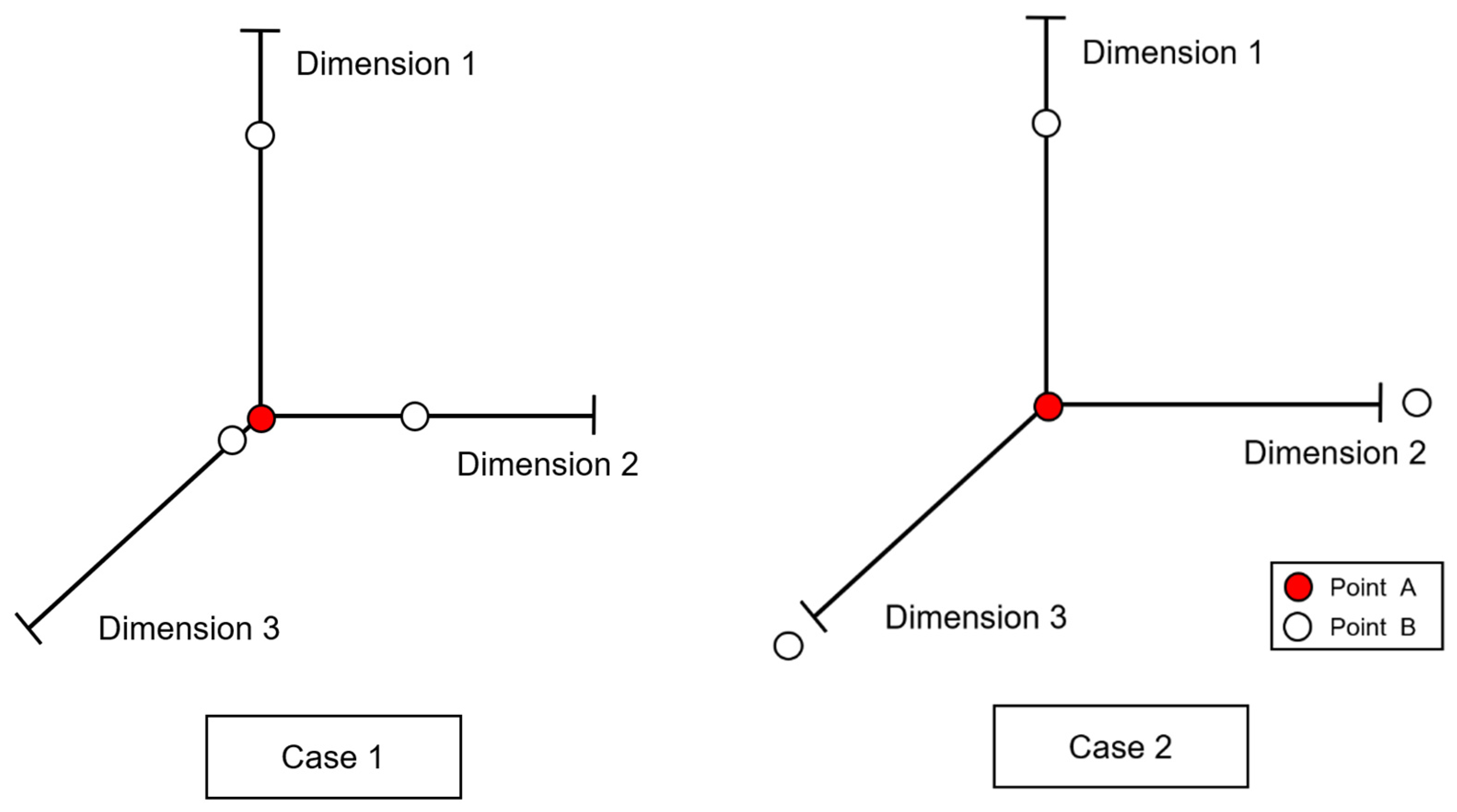
In this approach, the strictest way of defining a cluster is probably to calculate the density of points satisfying all criteria (i.e., closely located than Eps (k) in the k dimension for any k = 1, 2 … n + 2) and evaluate whether it is greater than MinPts. If this is too conservative, one may establish a tolerance that specifies the minimum number of epsilon parameters to be met, and a simulated annealing algorithm may be incorporated to adjust the tolerance. For the sake of simplicity, however, we will use the strictest definition in the rest of this paper.
Figure 1 illustrates two cases, one in which Point B is close to Point A in all dimensions and the other in which Point B is within the threshold for one dimension but not for the other two dimensions. In the former case, Point B is added to the numerator when calculating the point density around Point A. In the latter case, on the other hand, Point B would be ignored for the density estimation when using strictest rule.
One potential problem of this method is that the computational difficulties increase exponentially, as the method involves the construction of a (n + 2) dimensional distance matrix, where n is the number of non-spatial and non-temporal attributes. One way to work around this problem is to calculate the distance between each pair of points in turn, instead of completing the full distance matrix in advance. To evaluate the presence of a cluster around a specific point i, it is necessary to estimate the distance from i to the other (m − 1) points, where m is the number of observations in the data, but it is not necessary to determine, for example, the distance between pairs not including i, and points that are already in the cluster can be excluded from the distance calculation. Furthermore, if a point is not within the threshold distance in one dimension, the same point may not need to be considered in the other dimensions, thus reducing the number of calculations required.
This computational strategy may seem inefficient as some of the calculations will be duplicated. However, the distance calculations can be fully parallelized because each distance computation is independent; further, this approach can avoid making a set of m-by-m matrices, which are often too large to handle.
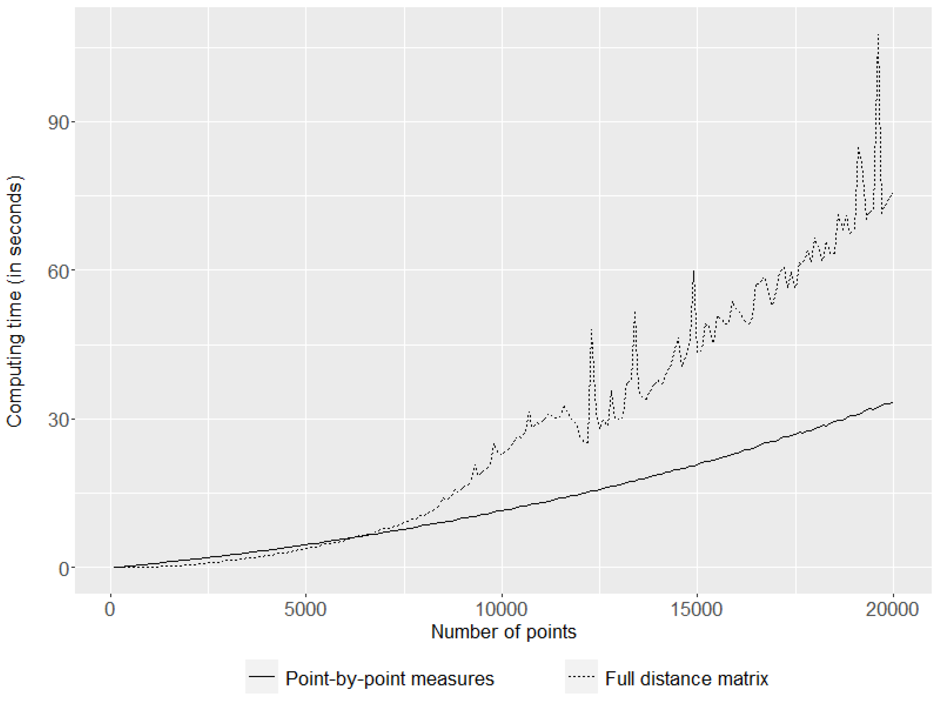
The two lines in Figure 2 represent the computation time for clustering when the full distance matrix is constructed in advance (dotted line) and when the distances are measured at each point repeatedly (solid line). The computation time was measured on an AMD Ryzen 5 3600 3.6 GHz CPU with 64 GB RAM, and the calculations were carried out in a single-core environment. The results show that the use of the full distance matrix requires less computation time when the number of observations is small (i.e., less than 6000 observations), but it seems to take considerable time even for moderately sized data. The point-by-point distance calculation, on the other hand, requires slightly more time when the data are small, but the rate of increase is much lower, making this method more suitable for large-scale data.
Table 1 presents the number of distance calculations needed to construct a full distance matrix for n points and compares them to the numbers of distance calculations when the point-by-point approach was adopted. The results are consistent with Figure 2: for a relatively small data set (i.e., 1000 points), the use of the full distance matrix appeared to be efficient, but as the number of points increased, the point-by-point approach involved fewer calculations. These results are of course dependent on the patterns of the data. If the points were arranged differently in space and time, the results could change significantly as well. As such, the point-by-point distance calculation does not necessarily reduce the computational complexity of the method, but it can confer a practical advantage, as illustrated in these examples.
Algorithm 1 below is the pseudocode describing how the method could be implemented (for working code, see the Supplementary Material section). In this work, the proposed method, MDST-DBSCAN, was written in R 4.0.3 in a Windows environment for accessibility, and its validity and efficiency were tested.
| Algorithm 1 MDST-DBSCAN Method |
| MDST-DBSCAN (D, Eps, Minpts) ## D = { Set of objects ## Eps = {} Set of thresholds ## Minpts = Minimum number of points to determine cluster Cluster_Label = 0 for = 1 to number of points If is not in a cluster For = 1 to number of attributes = distance from to other points in th attribute End For X = group of neighbors with (, , ) If number of objects in group X < Minpts mark as a noise Else Cluster_Label = Cluster_Label + 1 For = 1 to number of objects in group X mark all object in group X as a Cluster_Label End For For = 1 to number of objects in group X For = 1 to number of attributes = distance from to other points in th attribute End For Y = group of neighbors with (, , Eps 1, Eps 2 … Eps ) If number of objects in group in X > = Minpts mark all object in group Y as a Cluster_Label X = X union with Y End If End For End If End If End For End Algorithm |
4. Experiments
For cluster analysis, it is important to evaluate whether clusters detected using a specific method are naturally distinct groups or just artifacts of the method [16]. In this section, we will compare the clustering results from the proposed method to those from 4D + SNN to validate the accuracy and efficiency. The following subsection applies the proposed method to two idealized patterns from the Chameleon data set; the subsequent subsection utilizes real estate transaction data from Seoul, which contain multiple variables, including the xy coordinates and timestamps.
4.1. Idealized Patterns
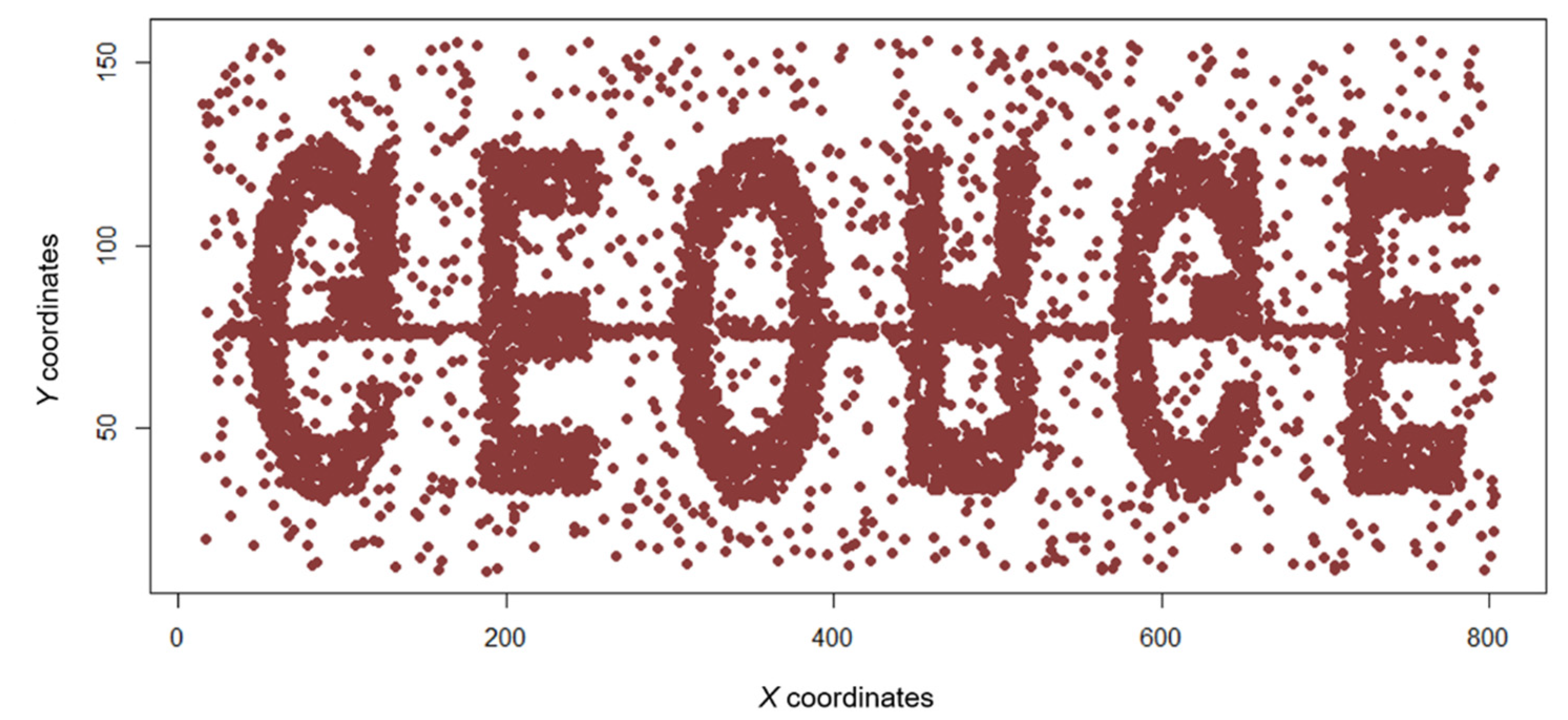
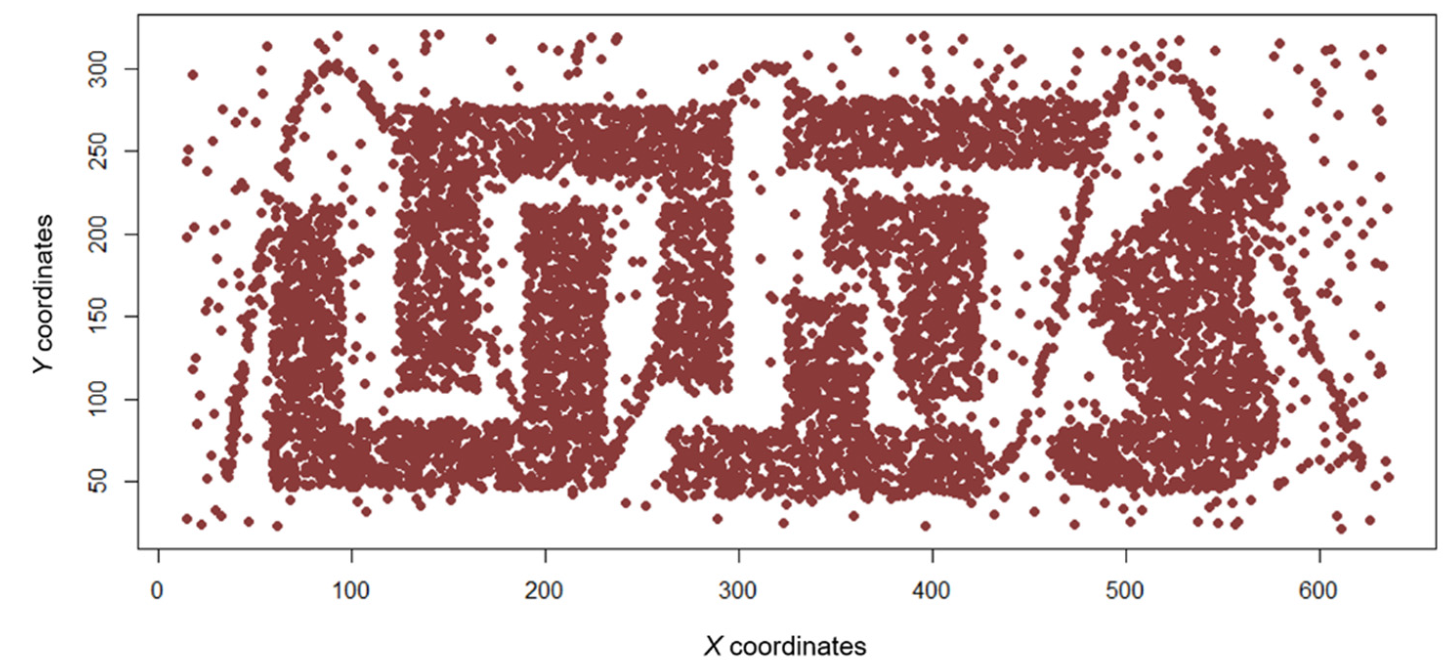
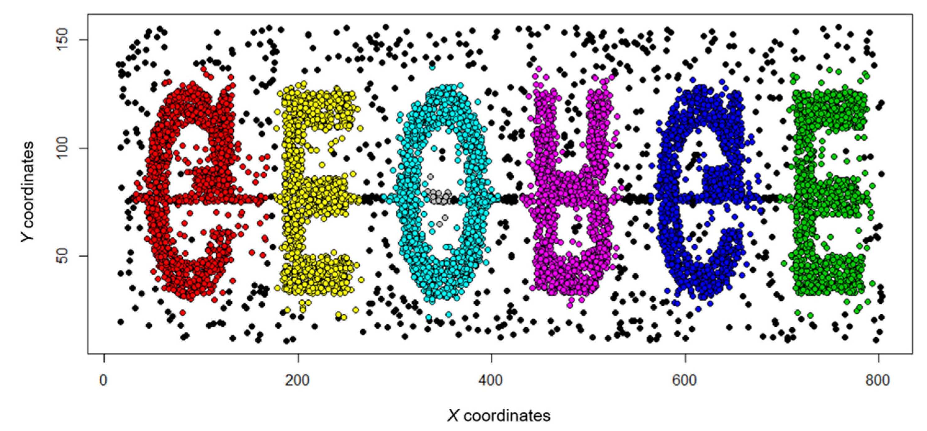
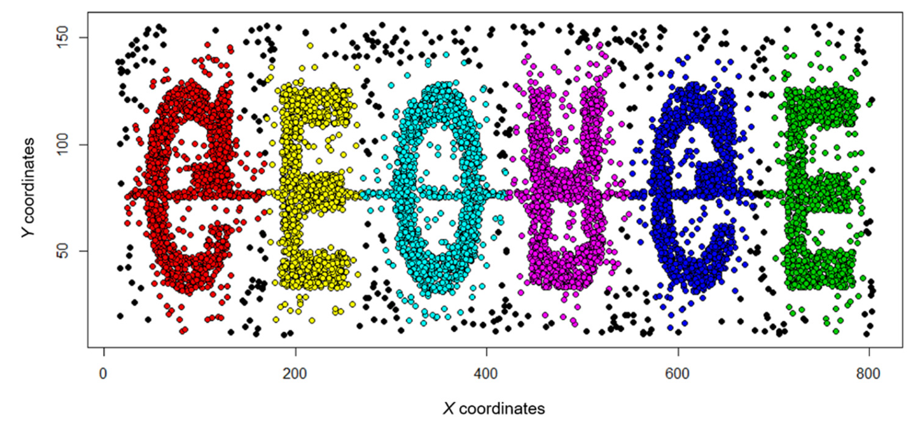
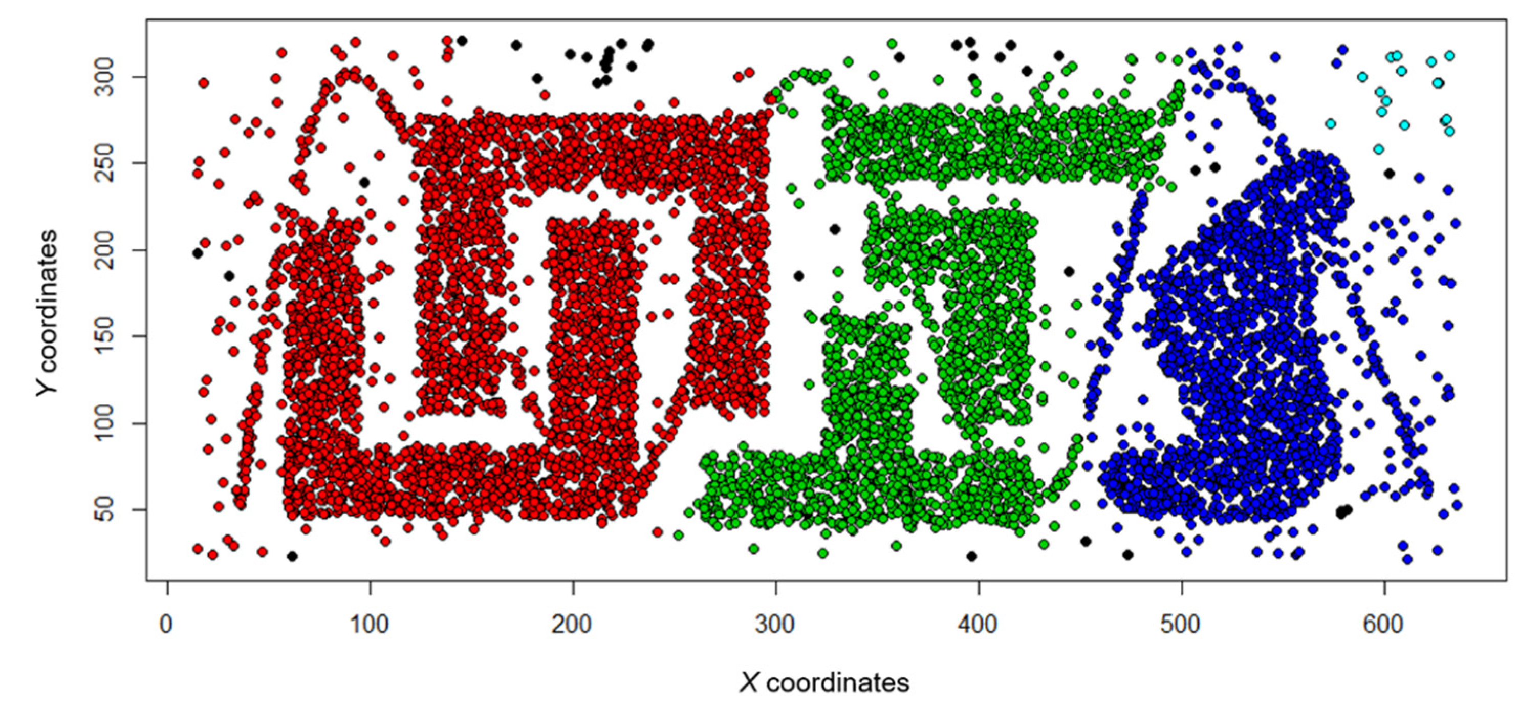
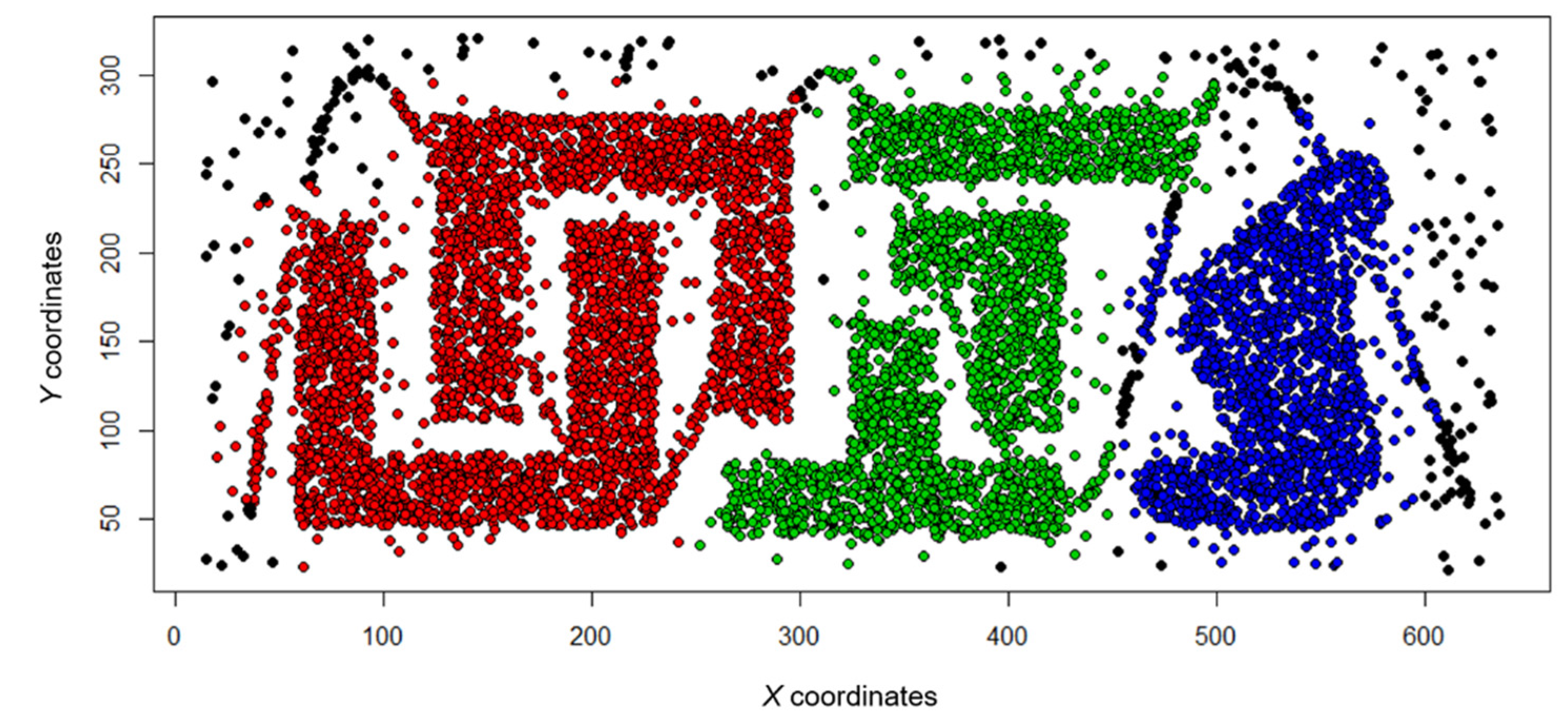
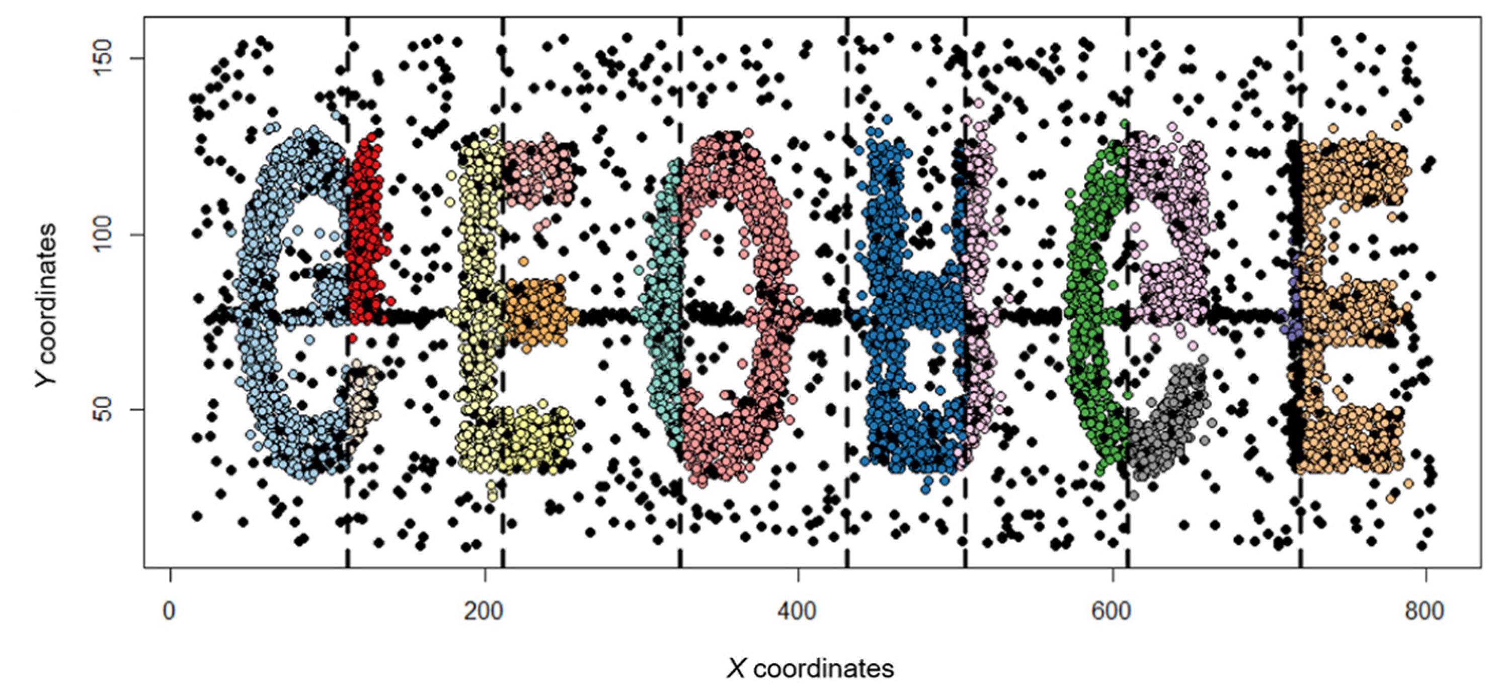
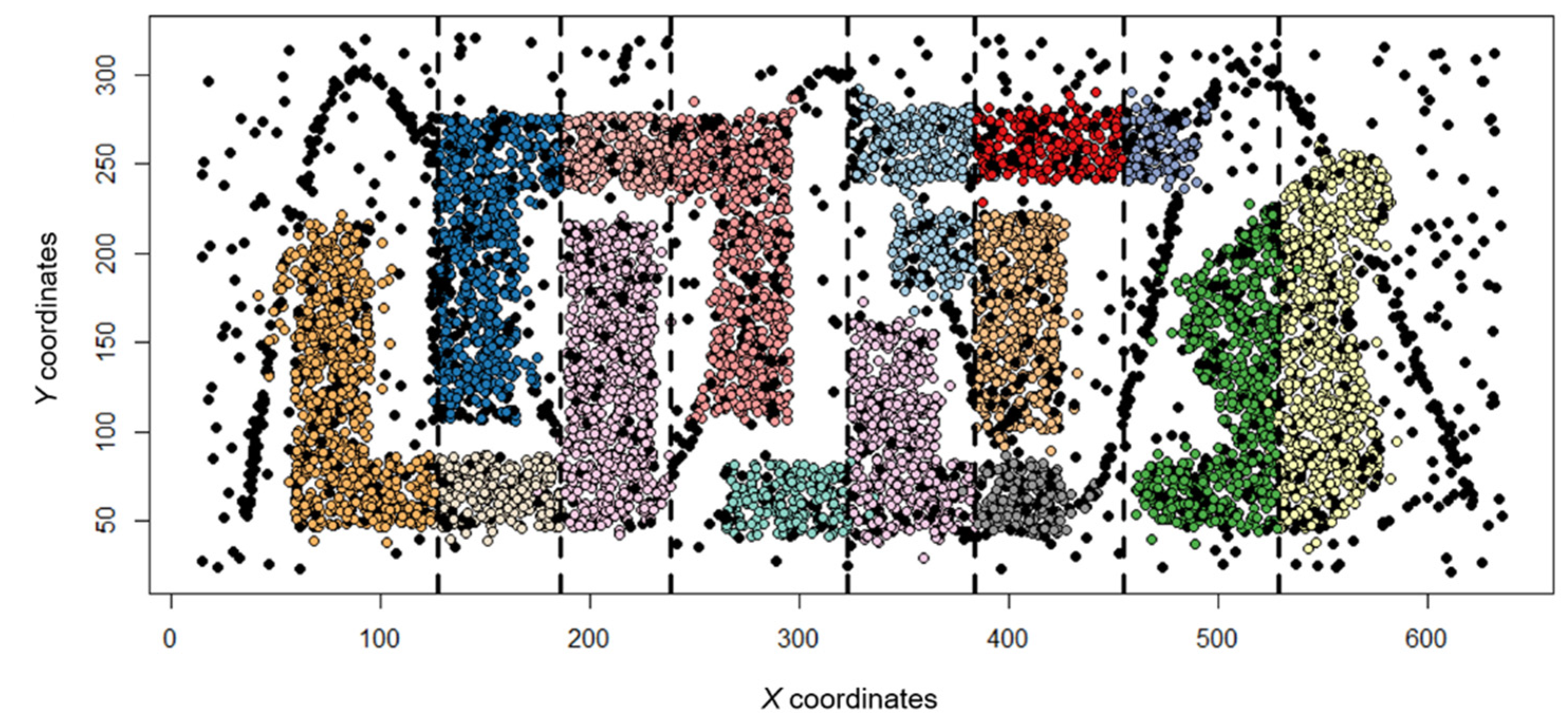
The Chameleon data set is popularly used to benchmark clustering methods. In this work, we will use two subsets of Chameleon, t5.8k and t4.8k [24,25], and their spatial arrangements are displayed in Figure 3 and Figure 4, respectively.
Since the Chameleon data set has no variables other than the spatial coordinates, as shown in Figure 3 and Figure 4, it is unsuitable for multidimensional spatio-temporal clustering. Thus, a modification was made to add temporal and additional synthetic variables for each data set. First, the points were classified according to the locations where the points were concentrated, and different temporal variables were entered. In each group, an integer representing the date was entered. The values were the same inside each group, but the values between the groups were different. Second, the entire data set was partitioned into groups of 1000 points according to the x-coordinates of the points, and the synthetic variable values were added depending on the group. Based on a 5.8k data set with 8000 points, for example, for the 1000 points with the smallest x-coordinate values, we added random numbers with a mean of 100 and a standard deviation of 10 as the synthetic variable values. Second, for the 1000 points in the group with the second smallest x-coordinate values, we added random numbers with a mean of 200 and a standard deviation of 10. The remaining points’ variables were added in the same way.
In cluster analysis, it is essential to choose the correct values of parameters as they can significantly influence cluster results. If the values are entered improperly, the resulting cluster may cover excessive range, or an overly small cluster may be established, from which it is hard to derive meaningful conclusions. Our proposed method, MDST-DBSCAN, mainly requires two main types of parameters, Eps and MinPts. This study uses K-Nearest Neighbor (KNN) distance plots to choose a value of Eps and uses the number of variables to choose a value of MinPts. In general, to derive an ideal threshold through the KNN distance plot, the location where the slope of the curve changes rapidly is used [8]. The location of rapid change indicates that outliers exist after the location in terms of distance between points. Thus, data with a value that exceeds this threshold is regarded as noise. If MinPts is set too high, an existing cluster may not be detected because too many neighbors are needed to form the initial cluster. A previous work proposed using a double number of the variables for choosing MinPts and argued that it was better to increase it according to the amount of noise in the clustering results [26].
Figure 5, Figure 6, Figure 7, and Figure 8 show the cluster analysis results using only spatial coordinates and temporal variables. Figure 5 and Figure 6 use the t5.8k data set, and Figure 7 and Figure 8 use the t4.8k data set, and each result was derived using 4D + SNN or MDST-DBSCAN. was All results confirmed that noise was concentrated in areas where the points were not dense and where the time variable was changed, but there was a slight difference. This difference occurs because the values of the parameters applied for each method cannot be set equally. In addition, the formation of similar clusters in both results indicates that the heuristic methods used to set the parameters in MDST-DBSCAN can be effectively used to confirm data similarity and to represent the differences between the clusters.
Figure 9 and Figure 10 show the results of cluster analysis using spatial coordinates, temporal variables, and additional virtual variables. Both results were derived using MDST-DBSCAN. The vertical lines in the figure denote the boundaries of the groups of 1000 points to which synthetic data changes were applied. The parameters used in the analysis were conducted similarly to the previous analysis. These results confirm that additional clusters were formed based on the vertical lines compared with the previous results using only time and space. In other words, it is possible to confirm the result of well-detected clusters using MDST-DBSCAN for additional variables. Similarly, this indicates that the method used for parameter setting is suitable for MDST-DBSCAN and that this method can divide clusters satisfactorily. In addition, when compared with the spatiotemporal clustering results, more data are identified as noise. We consider that this occurs as a result of an increase in the degree of similarity that can be included in the cluster with an increase in the number of dimensions to be considered. These results show that the threshold criterion needs to be lowered as the dimension increases when utilizing the MDST-DBSCAN method.
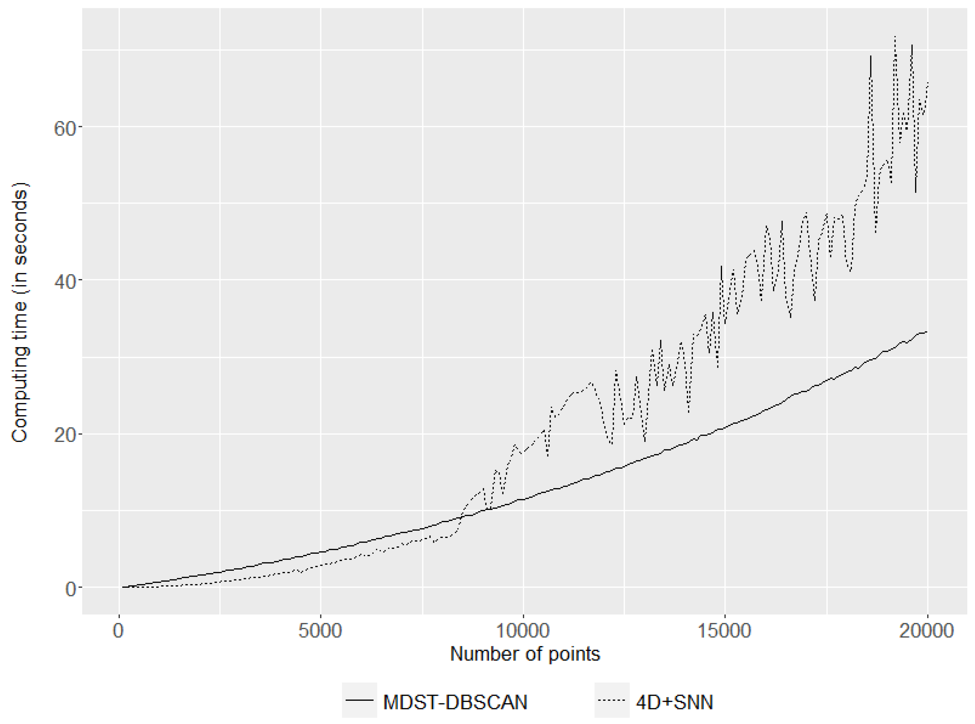
After comparing the clustering results, we compared the computation time for each method. Randomly generated point data were used to compare the computation times. Because the calculation time is expected to vary according to the number of points, the calculation time was measured until the number of points reached 20,000, starting with 50 points and increasing the number in intervals of 50. Spatial coordinates, temporal coordinates, and synthetic variables were all set to have uniform random distributions with values between 0 and 1. Each experiment was calculated in the same environment, and the results are shown in Figure 11. As confirmed in Figure 11, MDST-DBSCAN requires less time after the number of points used for analysis reaches approximately 7000. This reduction in computation time is considered to occur as a result of modifying the distance matrix computation method applied during the method modification process.
4.2. Real Data
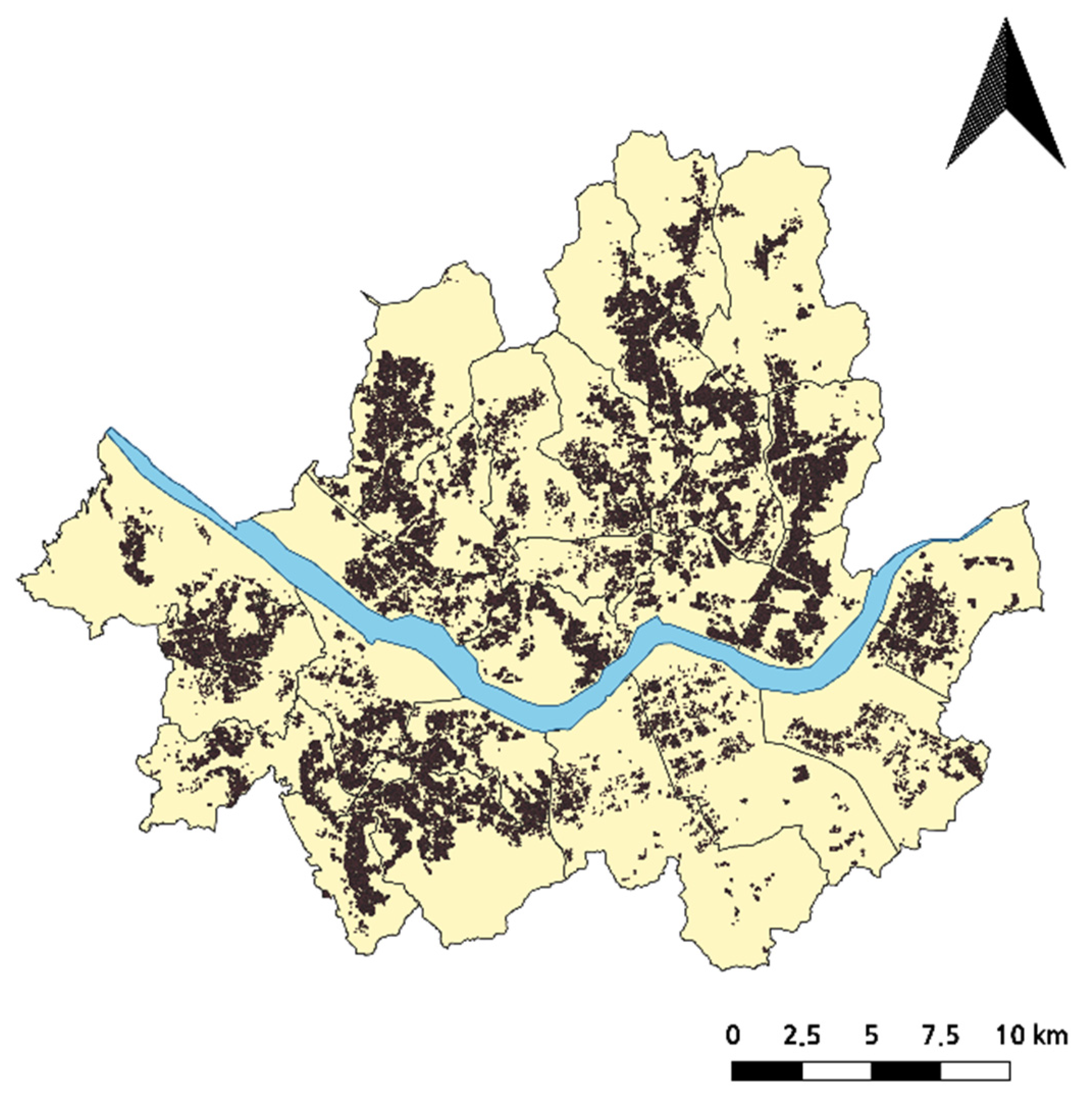
The real data used in the case study are the transaction data of detached houses in Seoul, Korea, from 2006 to 2018. Transaction data contain information on the building’s location, the price, the time, and other attributes of the building. These data include 108,481 points; the spatial distribution of the transaction data of detached houses is shown in Figure 12. In this section, we use the spatial, temporal, and price attributes of transaction data to evaluate the applicability of the MDST-DBSCAN method.
The density-based clustering method has great advantages in identifying clusters with arbitrary shapes [12,26,27,28]. The transaction data of detached houses constitute a massive data set and it is also presented without a specific spatial shape. Hence, it is considered suitable to utilize the proposed MDST-DBSCAN method. As in the idealized data case, the value of any given parameter was set using the KNN distance plot. However, unlike before, to find a more suitable parameter, we attempted to obtain better results by including some variations based on the KNN distance plot. Table 2 shows the parameters used in each analysis and the number and noise of clusters derived using these the parameters. Eps1 is the threshold for space, Eps2 is the threshold for time, and Eps3 is the threshold for price.
As the range of each threshold increases, the amount of noise decreases, and the number of clusters also decreases. In other words, as the threshold decreases, the number of points identified as neighbors increases as well, resulting in a decrease in the amount of noise and in small-sized clusters merging with each other during the process. That is, it is confirmed that although the attributes between data in the cluster are similar, there are cases where they belong to other clusters because of a slight difference.
Of course, analysis with various parameters is not sufficient to verify the results. Even if a good result is achieved by choosing various parameters, the quality of the result may be caused by coincidence. Therefore, we conducted a relative verification of the actually derived results through the CDbw (Composing Density between and with clusters) index [29]. CDbw is an index calculated through cluster density (compactness) and the degree of change within the cluster (intra change). The cluster density is defined using three elements: density within a cluster, density between clusters, and separation. In essence, it is a method of evaluating suitability for the clusters. As the index does not have an absolute criterion for interpretation, the relative size of the index is compared to determine which cluster is better. Data indicated as noise were excluded from the index calculation because such objects are represented as another cluster in the algorithm, which may distort the index calculation. For the index calculation, the distance between data variables is used. However, as the distance between the variables shows different distributions because of the unit problem, the index was calculated after standardization. The calculated CDbw index for each parameter is shown in Table 3.
When examining each index, the combination of parameters indicated in bold in Table 3 is considered to represent the most suitable type of cluster among the performed analyses. These results also show that the number of simple noise points and the number of clusters alone could not determine whether a cluster was properly formed.
Figure 13 shows the results of visualizing data based on the resulting clusters. The graphs on both sides show the transaction date and price according to the location. The color of the points is used to distinguish the clusters; both plots use the same color scale. For better visual clarity, only clusters with more than 300 points were used for the graph.
As shown in Figure 13, the x-axis and y-axis of the graph represent the place’s coordinates where the transaction occurred. The z-axis, which is the height, represents the transaction time and price. High z-axis values indicate recent transaction dates, or high prices in the respective graphs. In these results, the clusters corresponding to the latest times and the clusters farther in the past are divided. Similarly, the price results can be divided into high and low clusters. Through this, it can be confirmed that the house price increased as time passed in the corresponding space. In addition, in the case of transaction, there are no clusters in a certain region at the center of the entire period, which can be seen as empty. It has been confirmed that this phenomenon is caused by incidents that cause house prices to appear irregular, such as redevelopment projects, in the area. From these results, we can determine that the MDST-DBSCAN method has derived clusters suitable for the data.
5. Conclusions and Discussion
The advent of the era of big data era has increased the amount of data and the amount of information these data contain. This diversification of data increases the demand for researchers to build the knowledge inherent in the data. There are also many attempts and studies to identify clusters of multidimensional data in this trend. However, the methodologies developed in previous studies have mostly focused only on spatiotemporal dimensions; they do not consider additional variables. Furthermore, although clusters are formed in multiple dimensions, the elements used to form clusters are limited to specific variables. Hence, in this study, we proposed and implemented the MDST-DBSCAN method to cluster multidimensional data, including space and time.
In order to confirm the effectiveness of the proposed clustering method, we comparatively verified its results with a conventional multidimensional clustering method, 4D + SNN. The results were promising; the resulting shape and composition of the clusters were similar among the methodologies, and it was found that the use of the heuristic method of setting the parameters of the traditional DBSCAN method in the clustering process was effective. In addition, it was confirmed that an increase in computation time according to an increase in data size was more gradual in MDST-DBSCAN than in the traditional method. To introduce a practical application, we conducted a multidimensional spatiotemporal clustering analysis on the actual transaction price data of detached houses in Seoul, Korea. The result of this analysis indicated that the MDST-DBSCAN method was able to find the clusters suitable for the given conditions despite the large-scale data.
Despite its advantages, the proposed method has a limitation in that the method of defining the neighbors in the clustering process operates conservatively. In the current method, when detecting a neighboring point in the cluster formation process, the neighbor is determined only when the thresholds for all variables are satisfied. The more variables the data have, the fewer the cases that satisfy all thresholds, although this may vary depending on the data or the parameter settings. This leads to the conclusion that clustering in very high dimensions may be difficult with this approach. In addition, although the values do not significantly differ in forming clusters, there may be cases where clusters appear different from each other simply because the threshold was not satisfied. This limitation arises because a cluster formed with the current method is determined by a single factor, Eps, when setting the neighbors. Future research can further develop the method by setting additional factors or reflecting a fuzzy type of clustering method to determine neighbors.
This study’s foremost significance is proposing a multidimensional spatiotemporal clustering method that can be implemented while maintaining the traditionally reliable ST-DBSCAN method. This DBSCAN-based method is more straightforward and has less complexity than recent clustering methods (i.e., deep learning-based clustering methods). This difference makes it easier to interpret the results and makes it easier to understand the relationship between variables in the results. We believe that this may have advantages in terms of whether the method can explain the results or not in terms of eXplainable AI (XAI).
Nevertheless, to facilitate the use of the proposed method for real-world data, it needs to be improved in two main aspects. First, since MDST-DBSCAN requires many parameters, finding the right parameters becomes more challenging for researchers compared to the traditional approaches. As discussed in the previous section, the use of the KNN distance plot can help the parameter selection process to a certain extent, but such visual examination does not always reveal an ideal parameter value. Various alternative techniques have been offered to address this problem in recent years, and some efforts have been made to automate the parameter selection process. Although the existing state-of-the-art techniques are designed for DBSCAN [16], it would be possible to adjust these techniques and use them for the proposed method as well.
Second, in the current implementation of the proposed method, the clustering result will change significantly depending on which point is selected first in the clustering process. The impact of this characteristic may be another important point that needs to be evaluated and addressed in a future study.
Supplementary Materials
The code that implements MDST-DBSCAN is available from the following GitHub repository: https://github.com/locklocke/mdst-dbscan.
Author Contributions
Changlock Choi contributed to conceptualization, methodology, software, formal analysis, and visualization; Changlock Choi and Seong-Yun Hong wrote the paper; Seong-Yun Hong further revised and edited the paper. Both authors have read and agreed to the published version of the manuscript.
Funding
This work was supported by the National Research Foundation of Korea (NRF) grant funded by the Korean government (MSIT) (2019R1C1C1006555).
Conflicts of Interest
The authors declare no conflict of interest. The funders had no role in the design of the study; in the collection, analyses, or interpretation of data; in the writing of the manuscript, or in the decision to publish the results.
References
- Ibrahim, M.R.; Haworth, J.; Cheng, T. Understanding Cities with Machine Eyes: A Review of Deep Computer Vision in Urban Analytics. Cities 2020, 96, 102481. [Google Scholar] [CrossRef]
- Batty, M. Urban Analytics Defined. Environ. Plan. B Urban Anal. City Sci. 2019, 46, 403–405. [Google Scholar] [CrossRef] [Green Version]
- Singleton, A.D.; Spielman, S.; Folch, D. Urban Analytics: Spatial Analytics and Gis, 1st ed.; SAGE Publications Ltd.: London, UK, 2018. [Google Scholar]
- Goodchild, M.F. Citizens as Sensors: The World of Volunteered Geography. GeoJournal 2007, 69, 211–221. [Google Scholar] [CrossRef] [Green Version]
- Janowicz, K.; Gao, S.; McKenzie, G.; Hu, Y.; Bhaduri, B. Geoai: Spatially Explicit Artificial Intelligence Techniques for Geographic Knowledge Discovery and Beyond. Int. J. Geogr. Inf. Sci. 2020, 34, 625–636. [Google Scholar] [CrossRef]
- Li, W. Geoai: Where Machine Learning and Big Data Converge in Giscience. J. Spat. Inf. Sci. 2020, 20, 71–77. [Google Scholar] [CrossRef]
- Hartigan, J.A.; Wong, M.A. Algorithm as 136: A K-Means Clustering Algorithm. J. R. Stat. Society. Ser. C (Appl. Stat.) 1979, 28, 100–108. [Google Scholar] [CrossRef]
- Ester, M.; Kriegel, H.; Sander, J.; Xu, X. A Density-Based Algorithm for Discovering Clusters in Large Spatial Databases with Noise. In Proceedings of the Second International Conference on Knowledge Discovery and Data Mining, Portland, OR, USA, 2–4 August 1996; AAAI Press: Palo Alto, CA, USA, 1996; pp. 226–231. [Google Scholar]
- Ward, J.H. Hierarchical Grouping to Optimize an Objective Function. J. Am. Stat. Assoc. 1963, 58, 236–244. [Google Scholar] [CrossRef]
- Sneath, P.H.A. The Application of Computers to Taxonomy. Microbiology 1957, 17, 201–226. [Google Scholar] [CrossRef] [Green Version]
- Ankerst, M.; Breunig, M.M.; Kriegel, H.; Sander, J. Optics: Ordering Points to Identify the Clustering Structure. In Proceedings of the 1999 ACM SIGMOD International Conference on Management of Data, Philadelphia, PA, USA, 31 May–3 June 1999; pp. 49–60. [Google Scholar]
- Birant, D.; Kut, A. St-Dbscan: An Algorithm for Clustering Spatial-Temporal Data. Data Knowl. Eng. 2007, 60, 208–221. [Google Scholar] [CrossRef]
- Shi, Z.; Pun-Cheng, L.S.C. Spatiotemporal Data Clustering: A Survey of Methods. ISPRS Int. J. Geo-Inf. 2019, 8, 112. [Google Scholar] [CrossRef] [Green Version]
- Milligan, G.W.; Cooper, M.C. Methodology Review: Clustering Methods. Appl. Psychol. Meas. 1987, 11, 329–354. [Google Scholar] [CrossRef] [Green Version]
- Jain, A.K.; Murty, M.N.; Flynn, P.J. Data Clustering: A Review. ACM Comput. Surv. 1999, 31, 264–323. [Google Scholar] [CrossRef]
- Everitt, B.; Landau, S.; Leese, M.; Stahl, D. Cluster Analysis. In Wiley Series in Probability and Statistics; Wiley: Hoboken, NJ, USA, 2011. [Google Scholar]
- Min, E.; Guo, X.; Liu, Q.; Zhang, G.; Cui, J.; Long, J. A Survey of Clustering with Deep Learning: From the Perspective of Network Architecture. IEEE Access 2018, 6, 39501–39514. [Google Scholar] [CrossRef]
- Oliveira, R.; Santos, M.Y.; Pires, J.M. 4d + Snn: A Spatio-Temporal Density-Based Clustering Approach with 4d Similarity. In Proceedings of the 2013 IEEE 13th International Conference on Data Mining Workshops, Dallas, TX, USA, 7–10 December 2013. [Google Scholar]
- Karim, M.R.; Beyan, O.; Zappa, A.; Costa, I.G.; Rebholz-Schuhmann, D.; Cochez, M.; Decker, S. Deep Learning-Based Clustering Approaches for Bioinformatics. Brief. Bioinform. 2020, 22, 393–415. [Google Scholar] [CrossRef] [PubMed] [Green Version]
- Lamb, D.S.; Downs, J.; Reader, S. Space-Time Hierarchical Clustering for Identifying Clusters in Spatiotemporal Point Data. ISPRS Int. J. Geo-Inf. 2020, 9, 85. [Google Scholar] [CrossRef] [Green Version]
- Jacquez, G.M. A K Nearest Neighbour Test for Space–Time Interaction. Stat. Med. 1996, 15, 1935–1949. [Google Scholar] [CrossRef]
- Schubert, E.; Sander, J.; Ester, M.; Kriegel, H.P.; Xu, X. Dbscan Revisited, Revisited: Why and How You Should (Still) Use Dbscan. ACM Trans. Database Syst. 2017, 42, 19. [Google Scholar] [CrossRef]
- Yanenko, O. Introducing Social Distance to St-Dbscan. In Proceedings of the 22nd AGILE Conference 2019, Limassol, Cyprus, 17–20 June 2019. [Google Scholar]
- Havens, T.C.; Bezdek, J.C. An Efficient Formulation of the Improved Visual Assessment of Cluster Tendency (Ivat) Algorithm. IEEE Trans. Knowl. Data Eng. 2012, 24, 813–822. [Google Scholar] [CrossRef]
- Karypis, G.; Han, E.; Kumar, V. Chameleon: Hierarchical Clustering Using Dynamic Modeling. Computer 1999, 32, 68–75. [Google Scholar] [CrossRef] [Green Version]
- Tork, H.F. Spatio-Temporal Clustering Methods Classification. In Proceedings of the 7th Doctoral Symposium on Informatics Engineering (DSIE’2012) 2012, Porto, Portugal, 26–27 January 2012. [Google Scholar]
- Chimwayi, K.B.; Anuradha, J. Clustering West Nile Virus Spatio-Temporal Data Using St-Dbscan. Procedia Comput. Sci. 2018, 132, 1218–1227. [Google Scholar] [CrossRef]
- Poelitz, C.; Andrienko, G.; Andrienko, N. Finding Arbitrary Shaped Clusters with Related Extents in Space and Time. In Proceedings of the EuroVAST 2010: International Symposium on Visual Analytics Science and Technology, Bordeaux, France, 8 June 2010. [Google Scholar]
- Halkidi, M.; Vazirgiannis, M. A Density-Based Cluster Validity Approach Using Multi-Representatives. Pattern Recognit. Lett. 2008, 29, 773–786. [Google Scholar] [CrossRef]
Figure 1.
Determining neighbors for data with three variables.

Figure 2.
Changes in computation time according to the number of points.

Figure 3.
Spatial distribution of the t5.8k dataset.

Figure 4.
Spatial distribution of the t4.8k dataset.

Figure 5.
Results of spatiotemporal clustering using 4D + SNN.

Figure 6.
Results of spatiotemporal clustering using MDST-DBSCAN.

Figure 7.
Results of spatiotemporal clustering using 4D + SNN.

Figure 8.
Results of spatiotemporal clustering using MDST-DBSCAN.

Figure 9.
Results of multidimensional spatiotemporal clustering using MDST-DBSCAN.

Figure 10.
Results of multidimensional spatiotemporal clustering using MDST-DBSCAN.

Figure 11.
Comparison of computation time of spatiotemporal clustering methodologies.

Figure 12.
Spatial distribution of detached house transactions in Seoul, 2006–2018.

Figure 13.
Visualization of clustering results using real transaction price data of detached houses.
Figure 13.
Visualization of clustering results using real transaction price data of detached houses.


Table 1.
Changes of number of calculations according to number of points.
| Number of Points | Full Distance Matrix | Point-by-Point Measures |
|---|---|---|
| 1000 | 499,500 | 593,729 |
| 2000 | 1,999,000 | 1,653,844 |
| 3000 | 4,498,500 | 3,272,894 |
| 4000 | 7,998,000 | 4,926,691 |
| 5000 | 12,497,500 | 7,078,463 |
| 6000 | 17,997,000 | 10,505,182 |
| 7000 | 24,496,500 | 12,642,423 |
| 8000 | 31,996,000 | 16,915,592 |
| 9000 | 40,495,500 | 19,595,839 |
| 10,000 | 49,995,000 | 23,317,681 |
Table 2.
Changes in clusters according to parameter changes.
| No. | Eps1 (Space) | Eps2 (Time) | Eps3 (Price) | Clusters | Noises |
|---|---|---|---|---|---|
| 1 | 400 | 3 | 25,000 | 510 | 32,583 |
| 2 | 400 | 3 | 35,000 | 481 | 26,312 |
| 3 | 400 | 3 | 45,000 | 460 | 22,753 |
| 4 | 400 | 6 | 25,000 | 257 | 19,052 |
| 5 | 400 | 6 | 35,000 | 214 | 14,189 |
| 6 | 400 | 6 | 45,000 | 195 | 11,616 |
| 7 | 500 | 3 | 25,000 | 323 | 23,733 |
| 8 | 500 | 3 | 35,000 | 292 | 18,188 |
| 9 | 500 | 3 | 45,000 | 271 | 15,171 |
| 10 | 500 | 6 | 25,000 | 157 | 13,379 |
| 11 | 500 | 6 | 35,000 | 116 | 9910 |
| 12 | 500 | 6 | 45,000 | 111 | 7928 |
Table 3.
CDbw index change with varying parameters.
| No. | Eps1 | Eps2 | Eps3 | Clusters | Noises | CDbw |
|---|---|---|---|---|---|---|
| 1 | 400 | 3 | 25,000 | 510 | 32,583 | 0.322 |
| 2 | 400 | 3 | 35,000 | 481 | 26,312 | 0.248 |
| 3 | 400 | 3 | 45,000 | 460 | 22,753 | 0.212 |
| 4 | 400 | 6 | 25,000 | 257 | 19,052 | 0.386 |
| 5 | 400 | 6 | 35,000 | 214 | 14,189 | 0.318 |
| 6 | 400 | 6 | 45,000 | 195 | 11,616 | 0.263 |
| 7 | 500 | 3 | 25,000 | 323 | 23,733 | 0.313 |
| 8 | 500 | 3 | 35,000 | 292 | 18,188 | 0.276 |
| 9 | 500 | 3 | 45,000 | 271 | 15,171 | 0.234 |
| 10 | 500 | 6 | 25,000 | 157 | 13,379 | 0.533 |
| 11 | 500 | 6 | 35,000 | 116 | 9910 | 0.334 |
| 12 | 500 | 6 | 45,000 | 111 | 7928 | 0.242 |
Publisher’s Note: MDPI stays neutral with regard to jurisdictional claims in published maps and institutional affiliations. |
© 2021 by the authors. Licensee MDPI, Basel, Switzerland. This article is an open access article distributed under the terms and conditions of the Creative Commons Attribution (CC BY) license (https://creativecommons.org/licenses/by/4.0/).
Share and Cite
MDPI and ACS Style
Choi, C.; Hong, S.-Y. MDST-DBSCAN: A Density-Based Clustering Method for Multidimensional Spatiotemporal Data. ISPRS Int. J. Geo-Inf. 2021, 10, 391. https://0-doi-org.brum.beds.ac.uk/10.3390/ijgi10060391
AMA Style
Choi C, Hong S-Y. MDST-DBSCAN: A Density-Based Clustering Method for Multidimensional Spatiotemporal Data. ISPRS International Journal of Geo-Information. 2021; 10(6):391. https://0-doi-org.brum.beds.ac.uk/10.3390/ijgi10060391
Chicago/Turabian StyleChoi, Changlock, and Seong-Yun Hong. 2021. "MDST-DBSCAN: A Density-Based Clustering Method for Multidimensional Spatiotemporal Data" ISPRS International Journal of Geo-Information 10, no. 6: 391. https://0-doi-org.brum.beds.ac.uk/10.3390/ijgi10060391
Note that from the first issue of 2016, this journal uses article numbers instead of page numbers. See further details here.