
Cycling Trajectory-Based Navigation Independent of Road Network Data Support

1
College of Surveying and Geo-Informatics, North China University of Water Resources and Electric Power, Zhengzhou 450046, China
2
State Key Laboratory of Geo-Information Engineering, Xi’an 710054, China
*
Author to whom correspondence should be addressed.
ISPRS Int. J. Geo-Inf. 2021, 10(6), 398; https://0-doi-org.brum.beds.ac.uk/10.3390/ijgi10060398
Submission received: 25 April 2021
/
Revised: 7 June 2021
/
Accepted: 7 June 2021
/
Published: 9 June 2021
Abstract
:The popularization of smart phones and the large-scale application of location-based services (e.g., exercises, traveling and food delivery via cycling) have resulted in the emergence of massive amounts of personalized cycling trajectory data, spurring the demand for map navigation based on cycling trajectories. Therefore, in the current paper, we propose a cycling trajectory-based navigation algorithm without the need for road network data support. The proposed algorithm focuses on extracting navigation information from a given trajectory and then guiding others to the destination along the original trajectory. In particular, the algorithm analyzes the coordinate and azimuth angle data collected by the built-in positioning and direction sensors of mobile smart phones to identify several turning modes from the provider’s cycling trajectory. In addition, the interference of the traffic conditions during data collection is considered in order to improve the recognition accuracy of the turning modes. The turning modes in the trajectory are subsequently transformed into navigation information and shared with users, so as to realize the shared navigation of the cycling trajectory. Experimental results indicate that the algorithm can accurately extract the turning feature points from cycling trajectory data, recognize various turning modes and generate correct navigation messages, thereby guiding users to arrive at the destination safely and accurately along the original trajectory. The algorithm is independent of electronic map platforms and does not require road network data support.
1. Introduction
The growing popularity of social networks has enhanced the demand for trajectory-based navigation, that is, sharing individual’s trajectory data with others, and navigating other trajectories based on the trajectory data themselves. Thus, in this paper, we propose a cycling trajectory-based route navigation algorithm that is independent of road network data support. The purpose of the algorithm is to identify the turning modes from a given cycling trajectory, convert the turning modes into navigation information, and share all this with other users.
As the core function of electronic maps, map navigation is closely related to the daily travel of map users. Traditional map navigation methods are typically reduced to the shortest path-finding problem, and their representative methods can be divided into two categories: label setting (e.g., the Dijkstra algorithm [1]) and label correction (e.g., the Bellman–Ford algorithm [2]). In order to speed up the calculation efficiency of the shortest path planning algorithm in large-scale networks, the authors of [3] propose the famous A* algorithm, with the aim of improving the search efficiency of the shortest path through heuristic searching. Based on multi-level and hierarchical characteristics of road networks, scholars have also proposed a series of the shortest path accelerated search methods based on multi-level road networks [4,5,6,7,8,9]. In addition to employing distance as an optimal condition, numerous studies have been performed to determine the shortest time path in a traffic network with dynamically changing weights, developing effective shortest time path planning algorithms in time-varying road networks [10,11,12,13,14,15,16,17,18].
With the expansion of social networks and smartphone popularity, path planning algorithms based on trajectory data have also flourished. For example, the authors of [19,20,21,22] propose intelligent route navigation algorithms that are consistent with human cognition via learning the experience and knowledge of taxi drivers. Additional path planning algorithms consider the individual’s familiarity with the route by analyzing individual trajectories [23,24]. The most popular route-finding algorithm is based on ant colony optimization via the analysis of massive personal trajectory data [25]. The authors of [26] are devoted to finding personalized paths based on drivers' preferences for driving trajectories. The authors of [27] provide tourists with personalized travel routes based on user interests, the duration of scenic spot visits, and how recent the visits were. In [28,29], personal travel preferences are considered based on the user’s historical trajectory in order to recommend personalized tourist routes.
A key challenge in trajectory sharing navigation is ensuring the independence of road network data. On the one hand, in addition to open-source electronic maps (e.g., OpenStreetMap), manufacturers of navigation electronic maps will not open road network data to developers, making it difficult to customize trajectory navigation functions. On the other hand, users generally prefer the trajectory-based navigation function in order to be independent of online map websites, which means it has cross-platform usability. Compared with traditional route navigation algorithms based on road networks, cycling trajectory-based route navigation algorithms are limited. The cycling navigation functions in traditional electronic maps are not able to support the recent emergence of massive cycling trajectories (food delivery by electric bicycle, cycling tourism, cycling exercise, etc.). Furthermore, individual demand for route navigation based on cycling trajectories is on the rise. Therefore, this algorithm has a very broad application space.
2. Algorithm Concept
In this section, we first define or explain some important terms.
Definition 1.
(Cycling Trajectory): The cycling trajectory T is a set of n consecutive positioning points of cycling vehicles (including bicycles, electric bicycles, motorcycles, etc.) in the order of time, namely. Each positioning point(∈0…n) is composed of triples (,,), whereandrepresent the longitude and latitude of the moving object at time, respectively.
Definition 2.
(Turning Feature Points): Turning feature points are important positioning points that are extracted from trajectory T by using a trajectory compression algorithm to reflect the turning behavior of the cycling vehicle, namely,(0 =, whereis a subset of T.
Definition 3.
(Turning Angle): Three consecutive turning feature points,,and, constitute two trajectory segments,and. The turning angle ofis the angle between vectorand. If turning feature pointis on the left-hand side of vector, the turning type at pointis a left turn; otherwise, it is a right turn.
Definition 4.
(Turn Sequence): The turn sequence is composed of a series of consecutive turning feature points with the same turning type. If the consecutive turning feature points(1 < j < k < m) all have the same turning type, then they constitute a turning sequence <>.
Definition 5.
(Turning Mode): The turning angles of every turning feature point in the turn sequence are summed up. According to the sum value, the turning mode is determined. The turning mode includes turn left, turn right, turn around, etc.
Definition 6.
(Navigation Message): Navigation message is the guidance information for cyclists at important turns, including turn left ahead, turn right ahead, turn around ahead, etc.
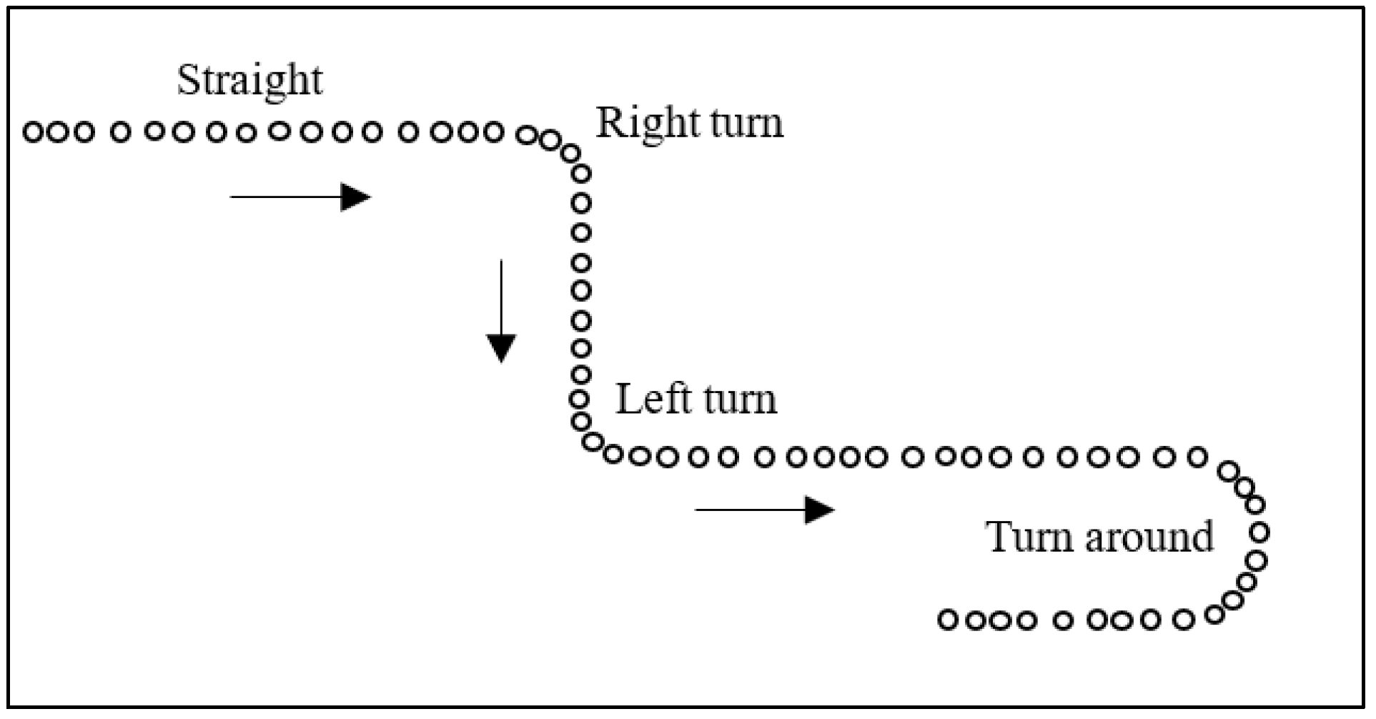
The proposed algorithm makes an important assumption: the cycling trajectory collected and shared by individual providers should completely comply with traffic rules, and thus there should be no traffic violations, such as retrograde, etc. Cycling trajectory-based navigation requires the extraction and sharing of important traffic information from a given cycling trajectory, such as going straight, left turn, right turn, turn around, etc. (Figure 1). Although the proposed algorithm does not require the support of road network data, the navigation route provider must carry the smart phone during cycling when collecting trajectory data. The algorithm recognizes and extracts the turning feature points based on the coordinate data collected by the positioning sensor, and subsequently combines the azimuth angle data of the direction sensor to further determine the turn modes, thus generating navigation messages to share with other users. The navigation route users are only required to collect the positioning coordinates of the trajectory via their mobile phone, not the direction data. The user is then able to reach their destination following the navigation messages. Cycling is more unpredictable than driving and is susceptible to numerous interferences. Therefore, a targeted algorithm is required. Moreover, cycling is also more flexible than driving; when the cyclist is found to deviate from the navigation route, they will be prompted to turn and can correct the route at any time. Consequently, the sharing navigation of cycling trajectories is completely feasible in practical applications.
3. Cycling Trajectory Sharing Navigation Based on Mobile Phone Sensors
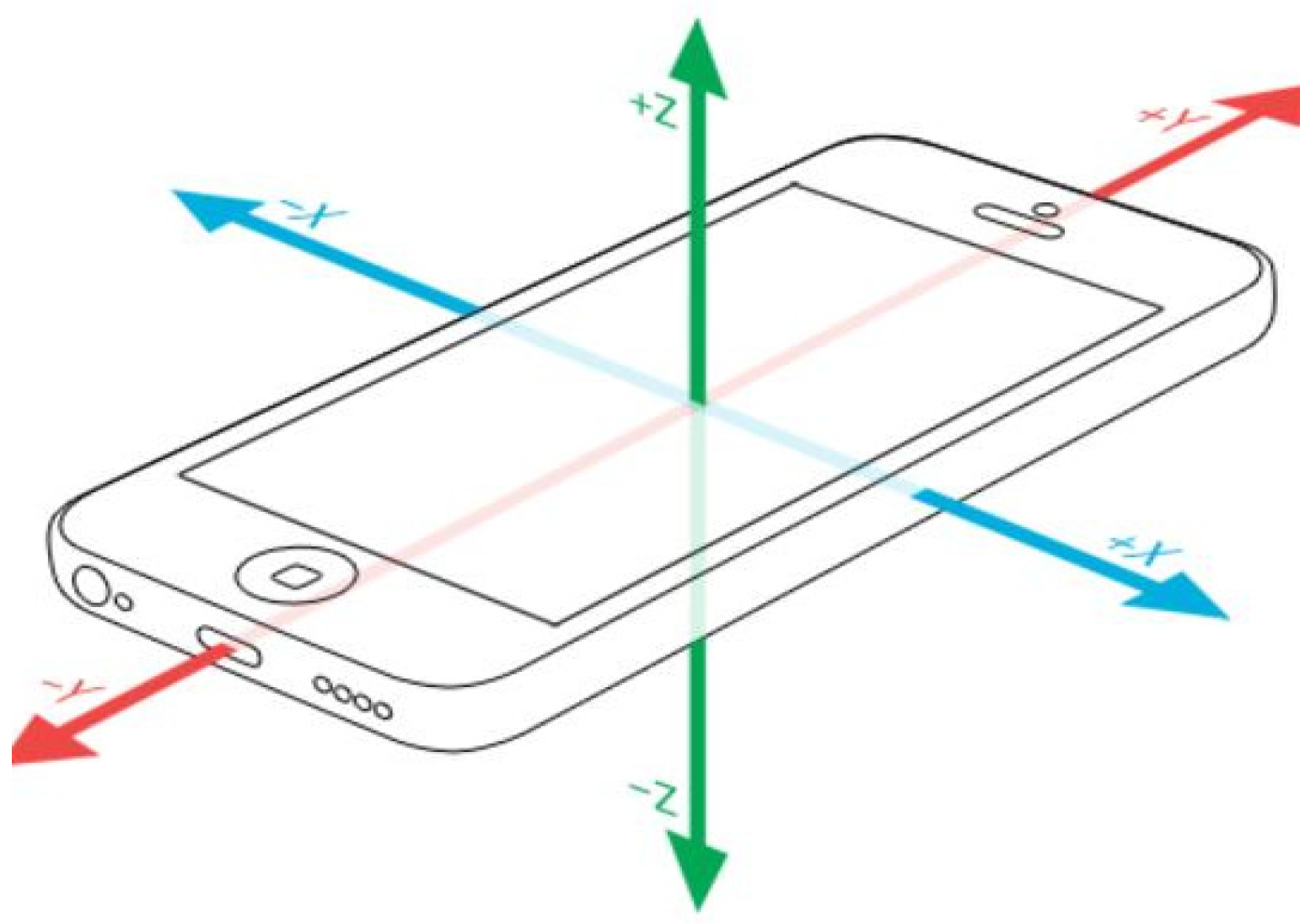
We set the sampling interval of the mobile phone positioning and direction sensors as 1000 ms and 30 ms, respectively. The direction sensor obtains the azimuth, pitch and roll angles (Figure 2). The azimuth angle is the angle between the positive direction of the Y-axis and the direction of the north pole of the geomagnetic field when the mobile phone rotates around the Z-axis; the pitch angle is the angle between the positive direction of the Y-axis and the horizontal direction when the phone rotates around the X-axis; and the roll angle is the angle between the positive direction of X-axis and the horizontal direction when the phone rotates around the Y-axis. The mobile phone must be fixed during data acquisition, while the initial posture of the mobile phone is unrestricted.
3.1. Preprocessing the Cycling Trajectory Data
The cycling trajectory data are processed via the following three steps: (i) removal of abnormal points; (ii) removal of staying points; and (iii) extraction of turning feature points.
When there are no GPS satellite signal, the collected coordinate data may deviate greatly from the actual coordinates, and thus abnormal points must be removed. Due to the low speed during cycling, the Euclidean distance between adjacent coordinate points will not be highly variable. If the difference in distance between the current and previous trajectory points is large, the trajectory point will be removed. Due to effects of GPS positioning errors, when the bicycle stops at a certain point, the coordinate data may drift back and forth to form a point cluster, which can be removed by a compression algorithm.
We employ the DP (Douglas–Peucker) algorithm for the trajectory compression to extract feature points and eliminate staying points. The algorithm, which uses the vertical deviation distance D as the threshold, first connects the start and end points of the trajectory data. The distance from other trajectory points to the line segment is then calculated to determine the point with the maximum distance : if < D, the intermediate points are removed; otherwise, the trajectory is divided into two sections based on this point. The procedure is repeated recursively for the two sections until there are no trajectory points between the first and last points.
3.2. Turning Mode Recognition in Cycling Trajectory Based on Mobile Phone Sensors
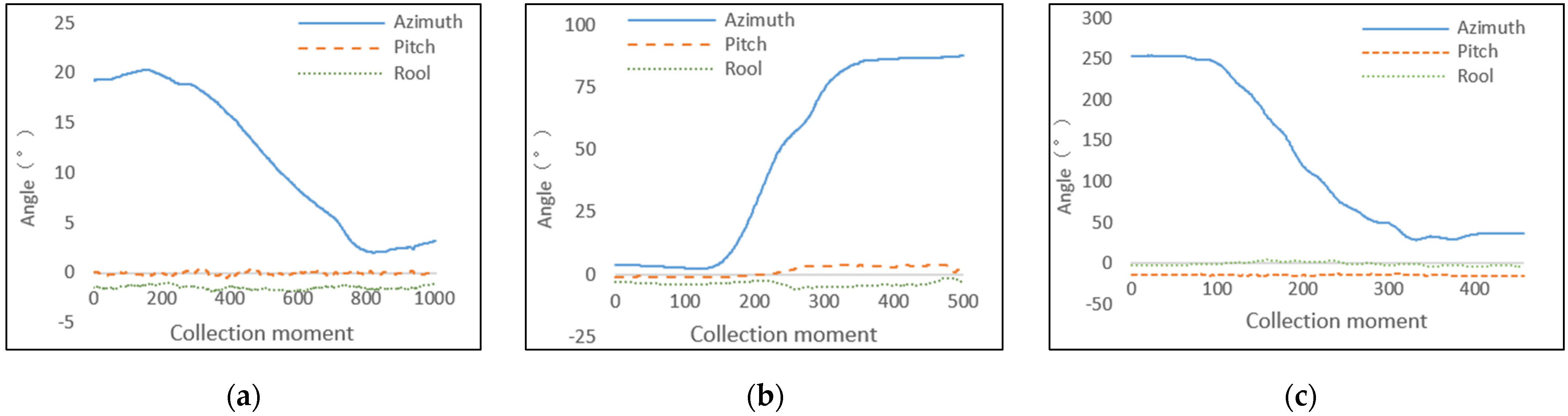
The spatial characteristics of the turning can be directly observed by visualizing the coordinate data collected via the positioning sensor. In general, as turning is performed, the angle between the adjacent trajectory segments will gradually transition from flat (cycling in a straight line) to obtuse (during turning). When turning ends, the angle becomes flat (cycling in a straight line) again. Based on this process, the turning sequence can be obtained. However, the coordinate data collected by the positioning sensor are not completely correct, as abnormal points may appear due to, for example, entering a tunnel without a satellite signal, or the obstruction of tall buildings. As a result, despite cycling in a straight line, the angle between the adjacent trajectory segments may be too acute. Therefore, in order to enhance the robustness of the algorithm, the positioning sensor is used as the principal sensor and the direction sensor is taken as the auxiliary. These two sensors are combined to comprehensively recognize turns. Figure 3 presents the variations in the three-axis data of the direction sensor during a 20° left turn (Figure 3a), a right 90° turn (Figure 3b) and a 180° turn (Figure 3c). The direction sensor of the mobile phone is able to accurately identify multiple turning phenomena. When the cycle turns, the pitch and roll angle do not change significantly, while the azimuth angle changes drastically. When the cycle turns right (left), the azimuth angle gradually increases (decreases), and the angle change is equal to the amplitude of the turn. The recognition of the turning mode in a cycling trajectory based on mobile phone sensors includes two key factors: the identification of turn sequences and the determination of turning modes.
3.2.1. Discovery of the Turn Sequence
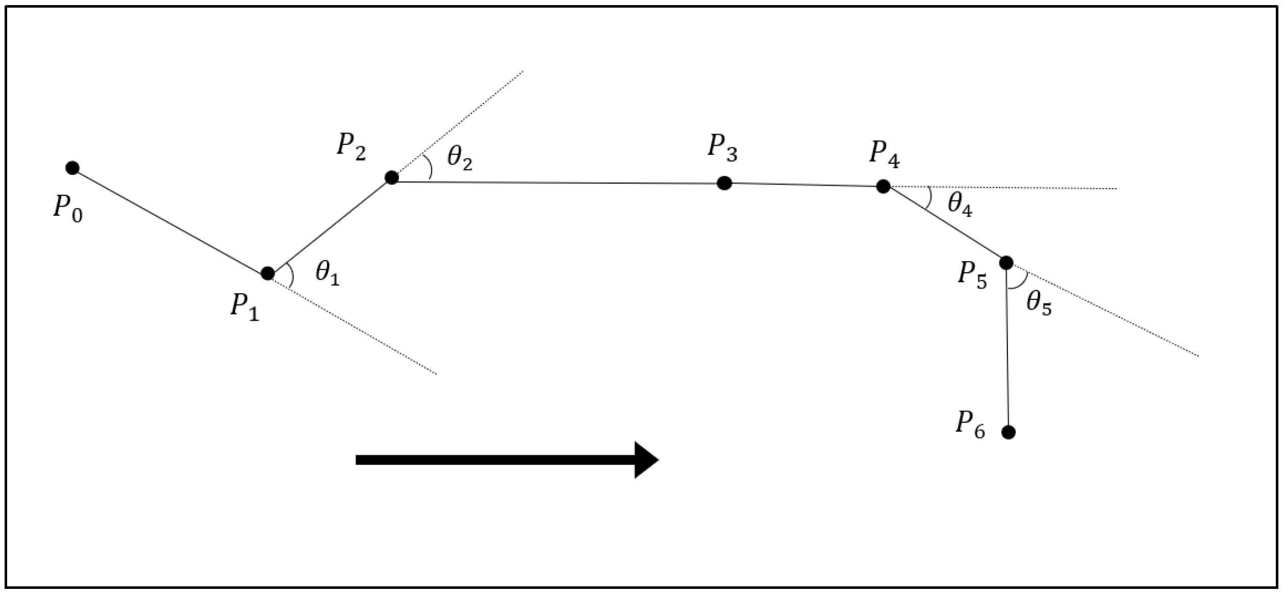
Figure 4 presents the method adopted to recognize turning sequences, which is composed of a series of turning feature points. The angles (∈1…n − 1) between vectors and , namely, the turning angles from line segment to line segment , can be described as:
where point set (0 = contains the turning feature points extracted by the trajectory compression algorithm. Angle threshold α and turning feature point distance threshold L are fixed. The thresholds α and L are the empirical parameters used in the program according to the inherent geometric characteristics of road features. The threshold α is used to distinguish a straight segment from a curved segment. The threshold L is used to merge two turns that are close together and to determine whether the current turn has been completed or not. If the turning angle at a turning feature point is greater than threshold , the point is added to the turning sequence. If point is on the left-hand side of vector , the turning type at point is a left turn, otherwise it is a right turn. Furthermore, if the next feature point simultaneously satisfies the following three conditions, it will continue to be added to the turning sequence: (i) the turning angle of the feature point is greater than the turning angle threshold ; (ii) the turning type of the feature point is equal to that of the previous feature point; and (iii) the distance between the current and previous feature points is less than distance threshold L. If the feature points do not satisfy the above conditions, the recognition of the turn sequence will stop and the recognition of the next turn sequence will continue. Figure 4 demonstrates three turn sequences, <>, <> and <>.
When cycling under tall buildings or in the shade of trees, the coordinate data collected by the positioning sensor may exhibit large errors. In particular, despite cycling in a straight line, the angle between adjacent trajectory segments may be too sharp. Therefore, the turn sequence recognition can be combined with the azimuth angle data of the direction sensor for an auxiliary evaluation. For example, in Figure 3, suppose that was originally a straight segment. Due to the large error of the collected coordinate data, <> and <> are mistakenly identified as turning sequences. In this case, the wrong turning sequence can be eliminated by combining with azimuth angle data. Taking the turning sequence <> as an example, we can obtain azimuth angles and of the trajectory points in the center of line segments and , respectively. If the turning angle determined via the coordinates is equal to the difference between and , the turn sequence is retained; otherwise, it is deleted.
3.2.2. Determination of Turning Modes
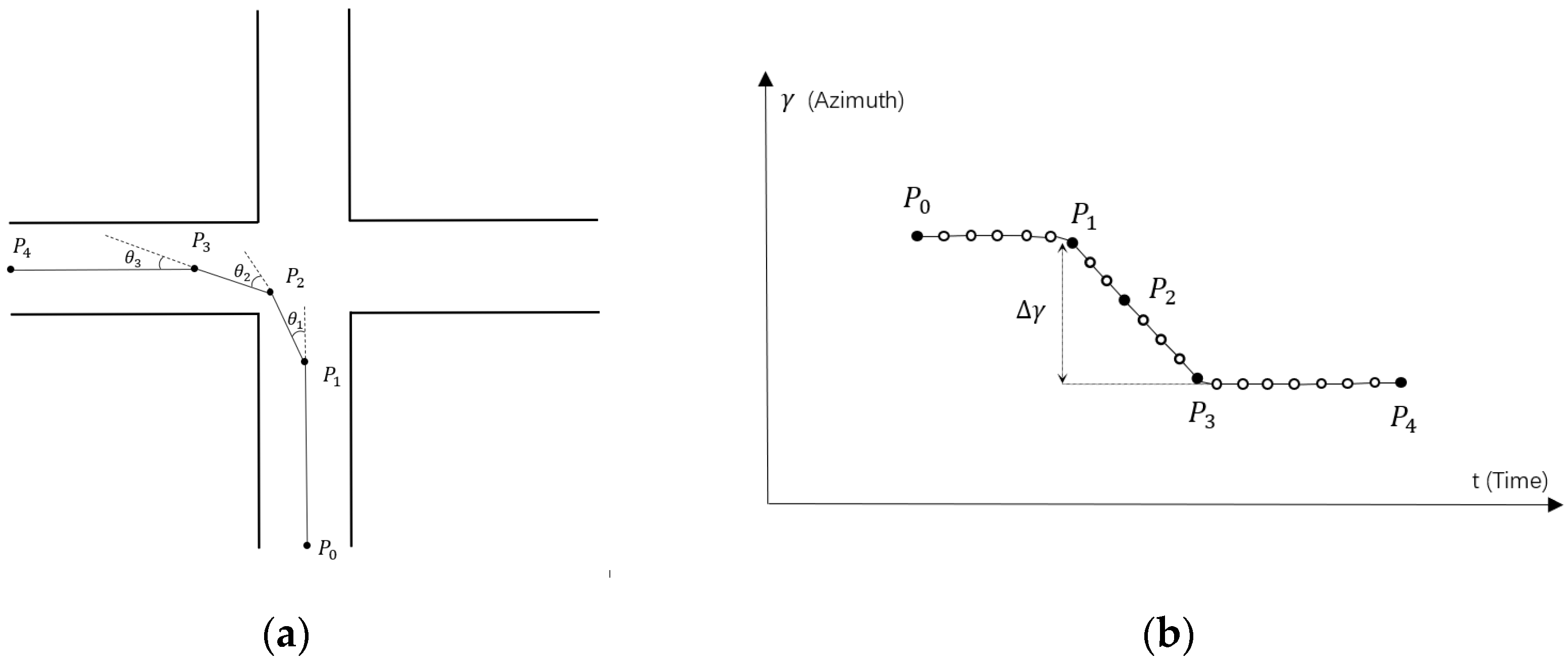
The turning mode can be determined by turning amplitude, which is calculated by accumulating turning angles in the turning sequence. For example, Figure 5a presents a series of trajectory feature points during a left turn, while Figure 5b depicts the corresponding azimuth angle change via the direction sensor. If we denote the extracted turning sequence as <, , >, where points and are the starting and ending points of the turning sequence, then and are the azimuth angles corresponding to the trajectory point at the center of segment and polyline segment , respectively. We subsequently determine the following three parameters: (i) the turning angle between and (Formula (1)); (ii) turning amplitude (the cumulative turning angles from point to (Formula (2))); and (iii) the azimuth angle difference between and (Formula (3)):
Under normal circumstances, , , and should be approximately equal, and can be used to determine the turning mode and turning amplitude. Moreover, and can be calculated using the trajectory point coordinates without data from the direction sensor. However, due to the potentially large errors of the GPS coordinates under adverse conditions, the azimuth angle data need to also be integrated into the calculation process for the auxiliary judgment. Therefore, the three parameters are employed to jointly determine the turning mode by taking the median of the three values as the whole turning amplitude.
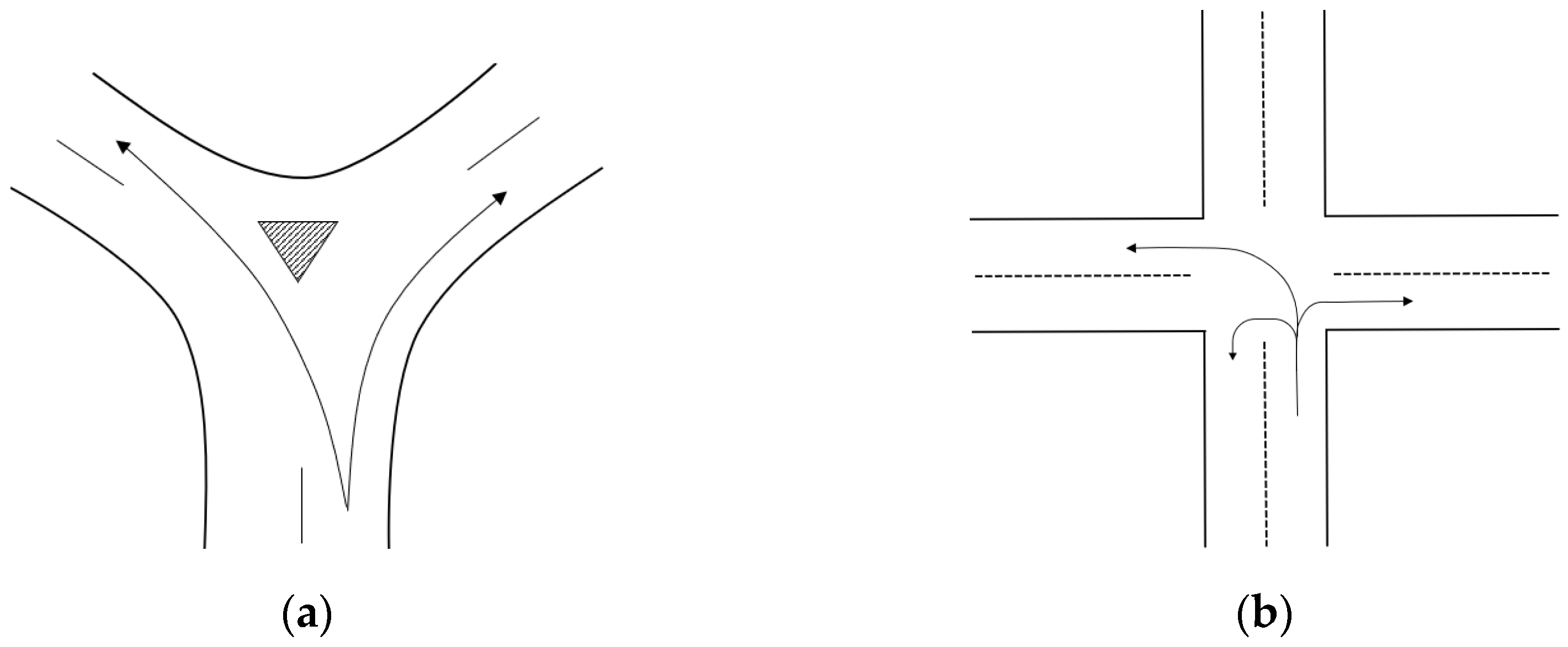
The turning range varies with the road intersection (Figure 6). For Y-shaped intersections (Figure 6a), the turning range lies within 30–60°, while for cross-shaped intersections (Figure 6b), the turning range is about . Therefore, when the turning range is between − and −, and , and − and , the navigation message is “turn left”, “turn right” and “go straight”, respectively. Additional turning ranges prompt “turn around”.
3.2.3. Recognition and Navigation of Complex Turning Mode
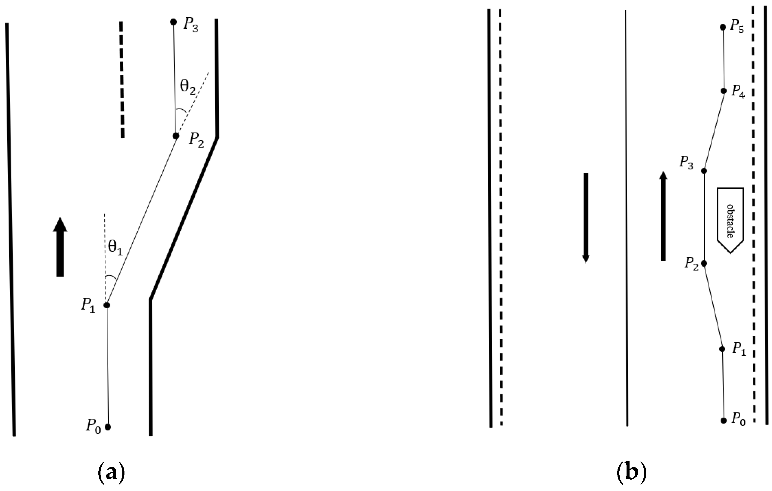
Cyclers often face complex traffic situations such as lane changing, narrowing or widening road surfaces (Figure 7a), and avoiding obstacles (Figure 7b). Thus, cycling trajectories typically exhibit many twists, resulting in small curves in the trajectory data. This can act as a false indication of a turn. However, the angles between the adjacent trajectory segments in these small curves are likely to be filtered through the trajectory compression algorithm due to their small size. Moreover, the accumulated turning angles are also likely to be small. For example, in Figure 7a, the directions of vectors and are almost the same, as are those of and , and hence they will not be misjudged as turns.
Despite the exclusion of small curves in the trajectory, complex traffic conditions can still lead to difficult turning modes. Here, we denote a turn mode as complex if the corresponding feature turning points with the largest turning angle in adjacent turn sequences are too close. In the following, we describe three typical examples. Figure 8a presents two adjacent turn sequences, represented by an initial right turn followed by moving straight for a short distance, and lastly, a left turn (unlike the change of lanes in Figure 7a). This example generally occurs on a narrow road. In Figure 8b, three consecutive turn sequences are represented on a circular road: a right turn, followed by a continuous left turn, and finally, a right turn. Figure 8c also depicts three consecutive turn sequences, represented by an initial left turn, followed by a right turn and a subsequent left turn, occurring on a large road intersection. In fact, Figure 8c denotes a left turn from to at the intersection, yet the turning process obviously violates traffic rules because one segment is retrograde. This is commonly observed in daily life. For these three special turning modes, the generated navigation message is distinct from that of normal turning modes.
We take Figure 8a as an example to describe the recognition of complex turning modes. Consider the two adjacent turning sequences <, > and <>. Point (red point in Figure 8a) is the feature turning point with the largest turning angle in turn sequence <, >, and (red point in Figure 8a) is another feature turning point with the largest turning angle in turn sequence <>. If the distance between and is less than threshold L, the adjacent two turning sequences <, > and <> constitute a complex turning mode. On arriving at point , the cyclist will receive the following navigation message: “turn right ahead and then turn left”. When three or more consecutive and close turn sequences are detected, such as those in Figure 8b,c, guiding users to follow the cycling trajectory proves to be a complicated task. Therefore, when the cyclist arrives to the complex turning area, the navigation message “need to turn ahead, please check the navigation route map” is sent to the user.
4. Cycling Trajectory-Based Sharing Navigation Algorithm
Unlike the problem of searching for optimal paths by merging multiple trajectories, as described in Ref. [19], the focus of this paper is extracting navigation characteristics from a single trajectory. The algorithm is applied to two situations: (1) By giving a user a shared cycling trajectory, other users follow the navigation route from the starting point of the trajectory to the end point of the trajectory. (2) Users directly input the start and end points, and we search all the cycling trajectories covering the start and end points from the trajectory database, and then recommend a certain trajectory to users according to some optimal criteria (shortest distance or shortest time), so that users can also arrive at the end point of the trajectory along the navigation route from the start point of the trajectory.
In the following, we provide the specific steps of the cycling trajectory sharing navigation algorithm. The cycling trajectory data collected by the provider include coordinate and azimuth angle data obtained by the positioning and direction sensors, respectively. The algorithm is divided into four key steps: (i) cycling trajectory data preprocessing; (ii) discovery of the turn sequences; (iii) determination of turning modes; and (iv) generation of the trajectory navigation message. Steps 1, 2 and 3 are all completed in the offline stage, and step 4 is route navigation in the online stage.
Step 1: Cycling trajectory data preprocessing
The DP algorithm is used for the trajectory compression to extract feature points and eliminate staying points. Since the GPS single-point positioning error is approximately 5-10 m, the vertical distance threshold D is set to 5 m.
Step 2: Discovery of turn sequences.
The turning angle threshold and turning feature point distance threshold L are set at this step. is set as to identify cycling in a straight line, while L is set as 30 m to adapt to different road intersection widths. Based on these two thresholds, the consecutive turning feature points should simultaneously satisfy the conditions described in Section 3.2.1. If these conditions are not satisfied, the turning sequence is considered to be over, and the discovery of the next turning sequence is continued.
Step 3: Determination of turning modes.
Section 3.2.2 describes the calculation of turning angle , cumulative turning angles , and the azimuth difference implemented to recognize the turning modes. The median of these three variables is taken as the turning amplitude. The navigation prompts also follow those provided in Section 3.2.2. The complex turning mode is subsequently recognized. If the distance between feature turning points with the largest turning angle in adjacent turn sequences is less than the 30 m threshold, the adjacent turn sequences constitute a complex turning mode.
Step 4: Generation of navigation messages.
The proposed algorithm obtains the user’s current location and outputs the corresponding navigation messages at the turns extracted from the provider’s cycling trajectory. Navigation messages of normal turning modes include “turn left”, “turn right” and “turn around”. Complex turning navigation messages include “turn right ahead and then turn left”, “turn left ahead and then turn right” and “need to turn ahead, please check the navigation route map”. When the user deviates from the navigation route, the navigation message is “you have deviated from the navigation route”.
5. Experimental Verification and Analysis
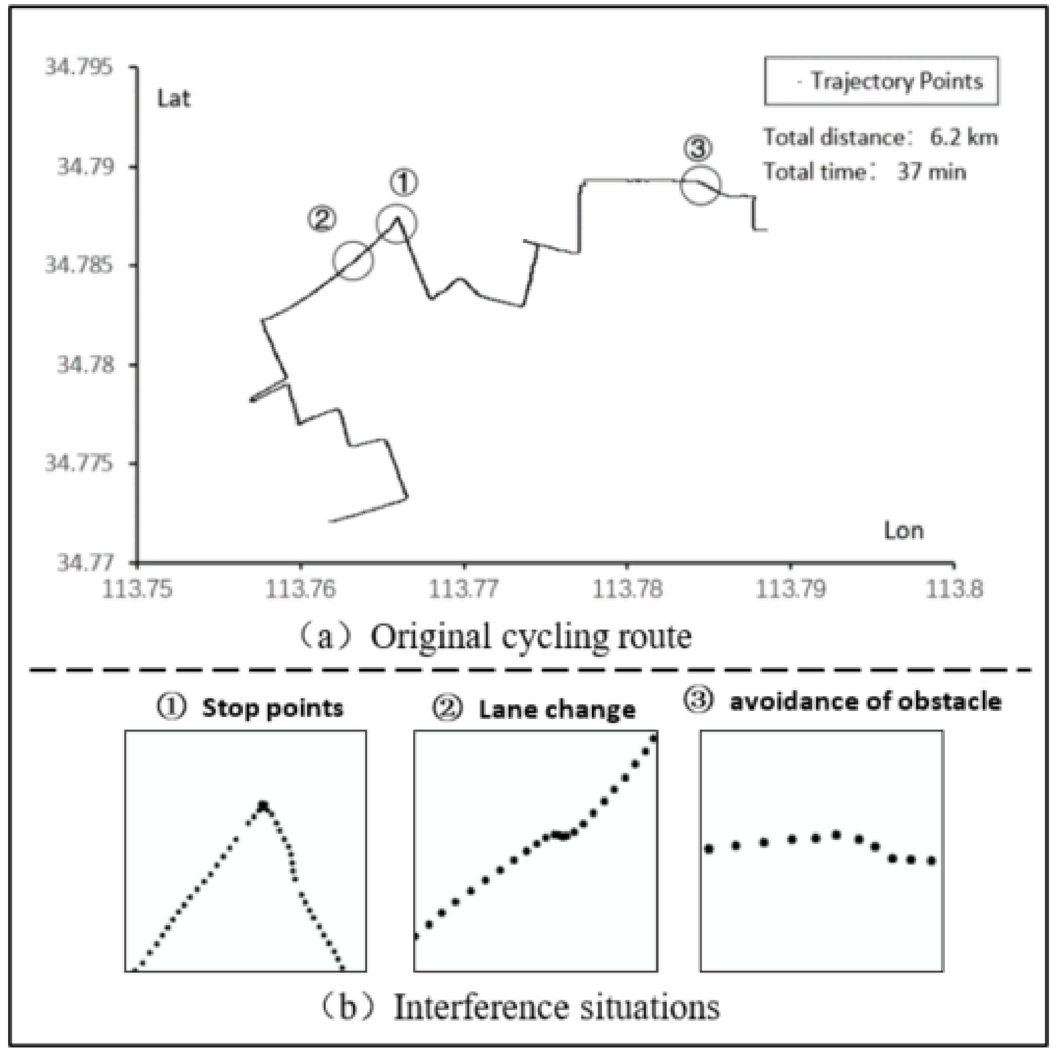
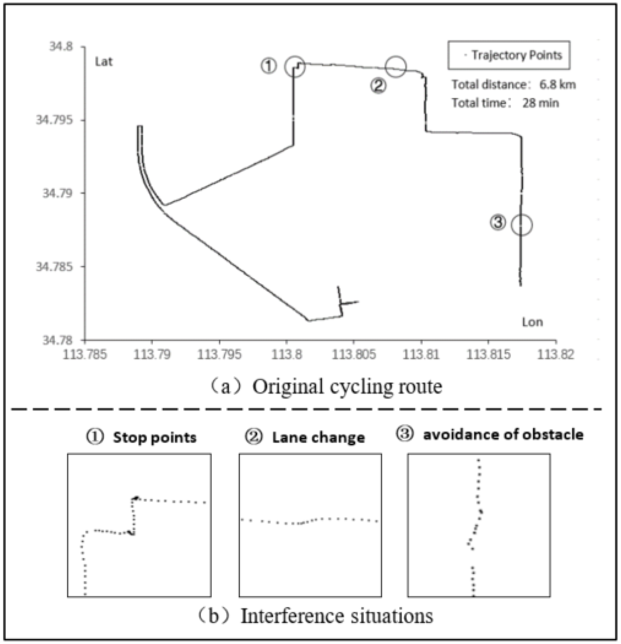
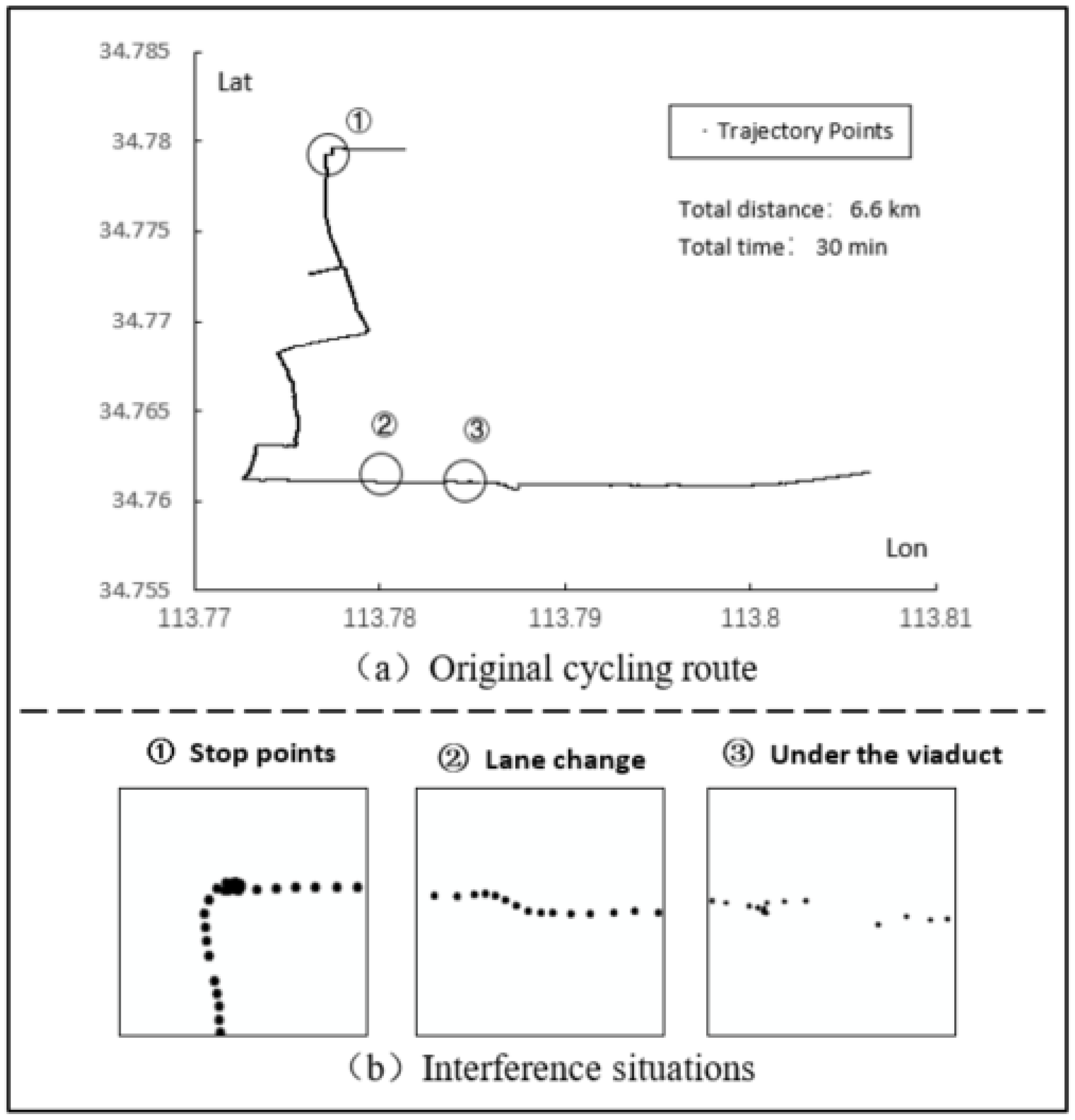
We adopt four types of smart phones to collect four trajectories, respectively (Figure 9, Figure 10, Figure 11 and Figure 12). The collected trajectories all include left and right turns, as well as turning around. Compared with driving trajectories, cycling trajectories are more easily disturbed by various traffic conditions. In order to ensure the representativeness of the experimental data and verify the actual effect of the algorithm, we include several complex traffic conditions during the data collection process. The examples also include various types of interference, such as staying at traffic lights, avoiding obstacles, changing lanes, and cycling under tall buildings or viaducts. Figure 9b, Figure 10b, Figure 11b and Figure 12b are partial enlarged views of the trajectory points in the circle frame of Figure 9a, Figure 10a, Figure 11a and Figure 12a, demonstrating the various interferences in the data collection process of the cycling trajectory.
5.1. Extraction Results of the Turning Feature Points
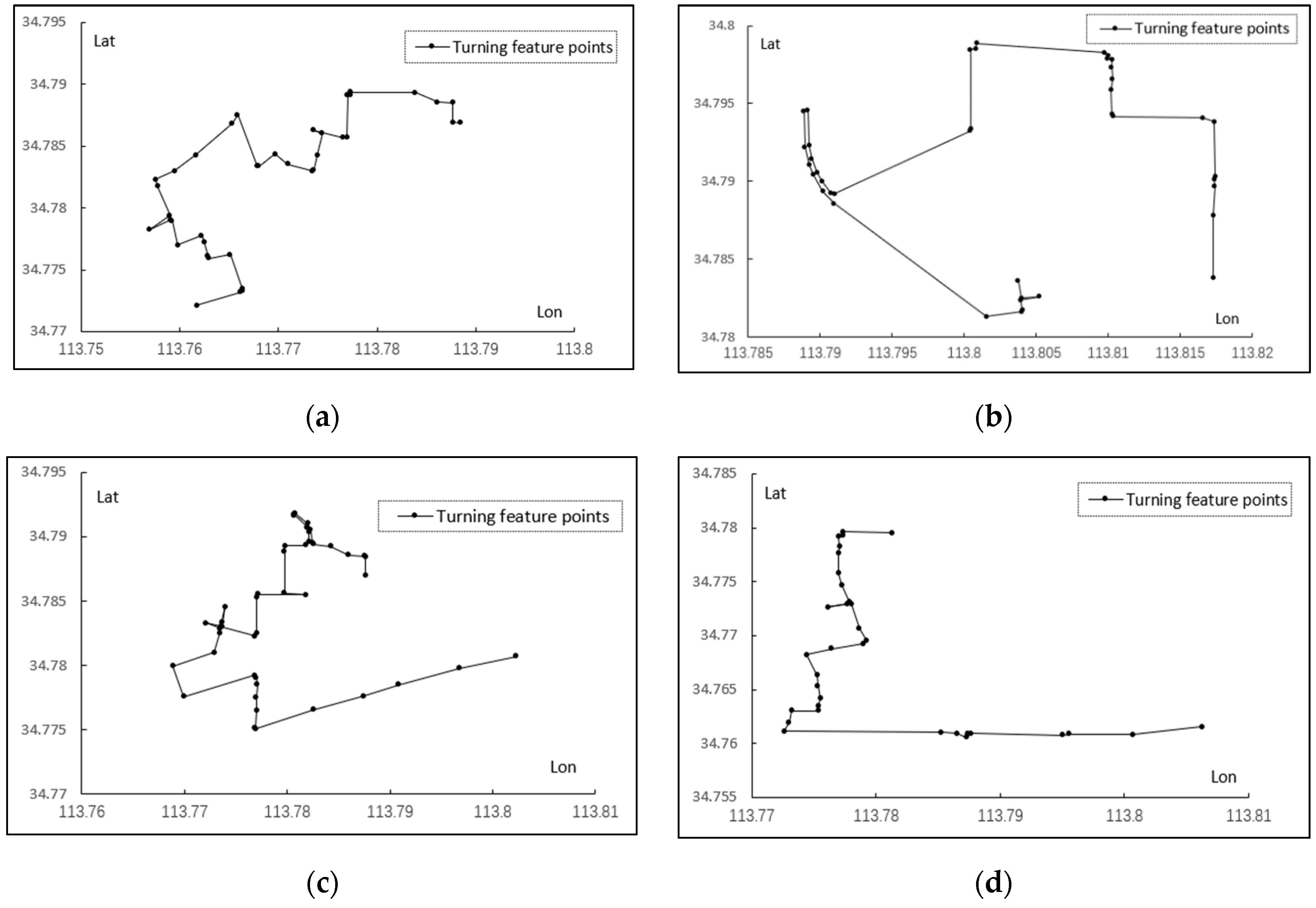
The turning feature points extracted via the compression algorithm based on the trajectory data should be consistent with the real turning points of actual roads. Table 1 reports the extraction of the turning feature points under different compression thresholds. When the compression threshold is set at 5–10 m, the drift and stop points in the trajectory data can be filtered out, while the extracted turning feature points are very close to the real turning points of the actual road. Figure 13 presents the turning feature point extraction under the 5 m compression threshold.
5.2. Experimental Results of the Trajectory Turning Mode Determination
The strength of the proposed algorithm is its ability to correctly recognize the turning information, even when the trajectory is disturbed by avoiding obstacles, lane changing and a weak GPS signal (e.g., from cycling under tall buildings and overpasses). As the accurate extraction of trajectory feature points is closely related to the recognition accuracy of the algorithm, the experiments verify the turning mode recognition accuracy across different compression thresholds (Table 2, Table 3, Table 4 and Table 5). Under different compression thresholds, the recognition accuracy of the turning modes based on the coordinate and azimuth data fusion is higher than that of just relying on coordinate data. In addition, the number of false and missing recognition instances is also lower. When the coordinate and azimuth data are combined, the recognition of the turning modes at compression thresholds of 5 or 7 m is the most consistent with the actual road conditions, and is higher than for compression thresholds of 3 or 10 m. Therefore, the compression threshold of the proposed algorithm should be set as 5 to 7 m for the sharing of cycling trajectories for navigation.
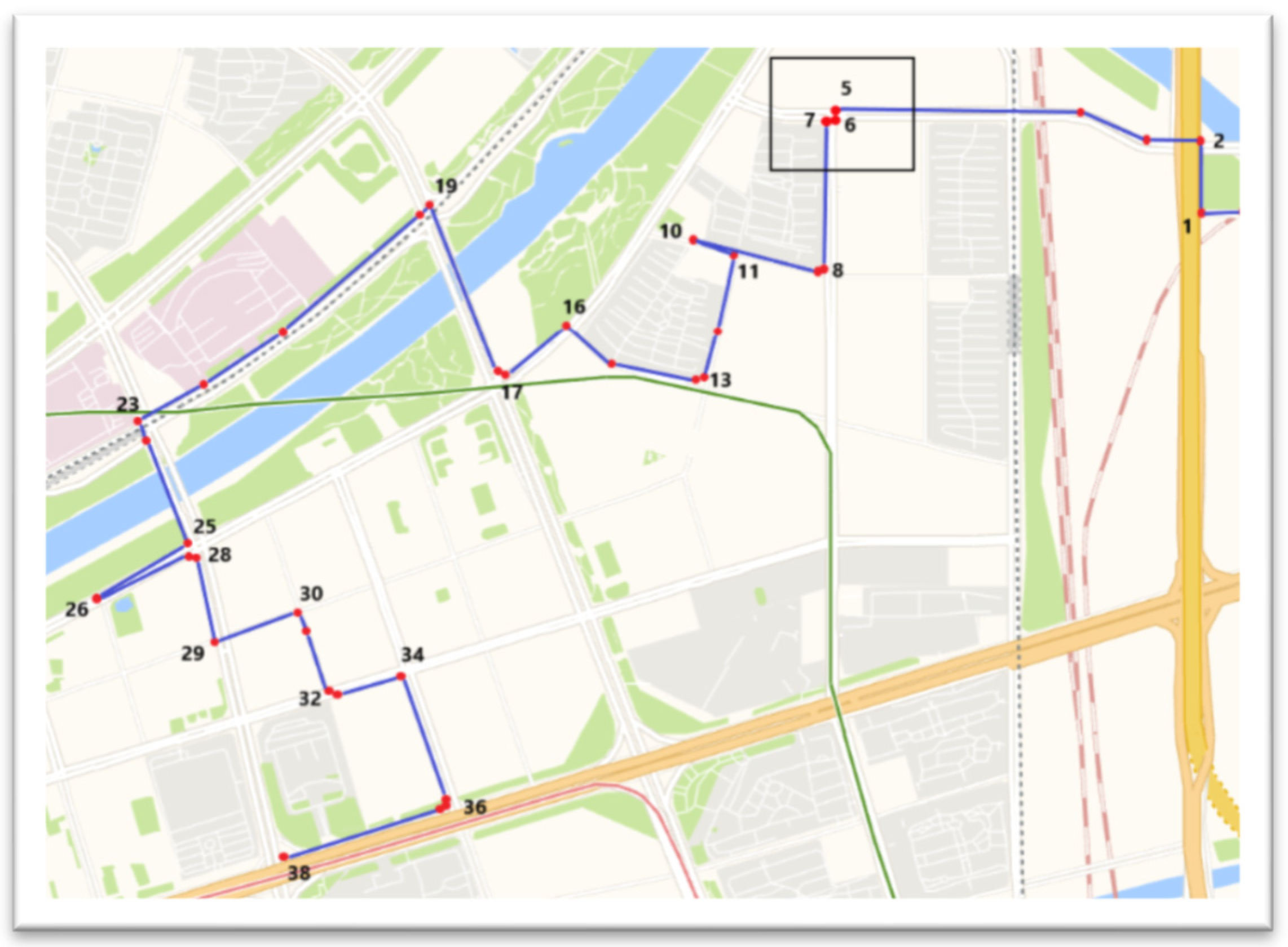
Although our algorithm does not rely on road network data for navigation, in order to verify the correctness of the algorithm, the first trajectory is taken as an example to compare the turning mode recognition results of the algorithm with the real turning modes of the actual road network (Figure 14). The compressed trajectory data are observed to correctly reflect the turning information of the actual road network. Note that the box in Figure 14 is a result of the three very short consecutive turn sequences, constituting complex turns. Table 6 compares the results between the turning modes extracted via this algorithm and those of the actual road network.
5.3. Generation of Trajectory Navigation Message and Navigation Experimental Results
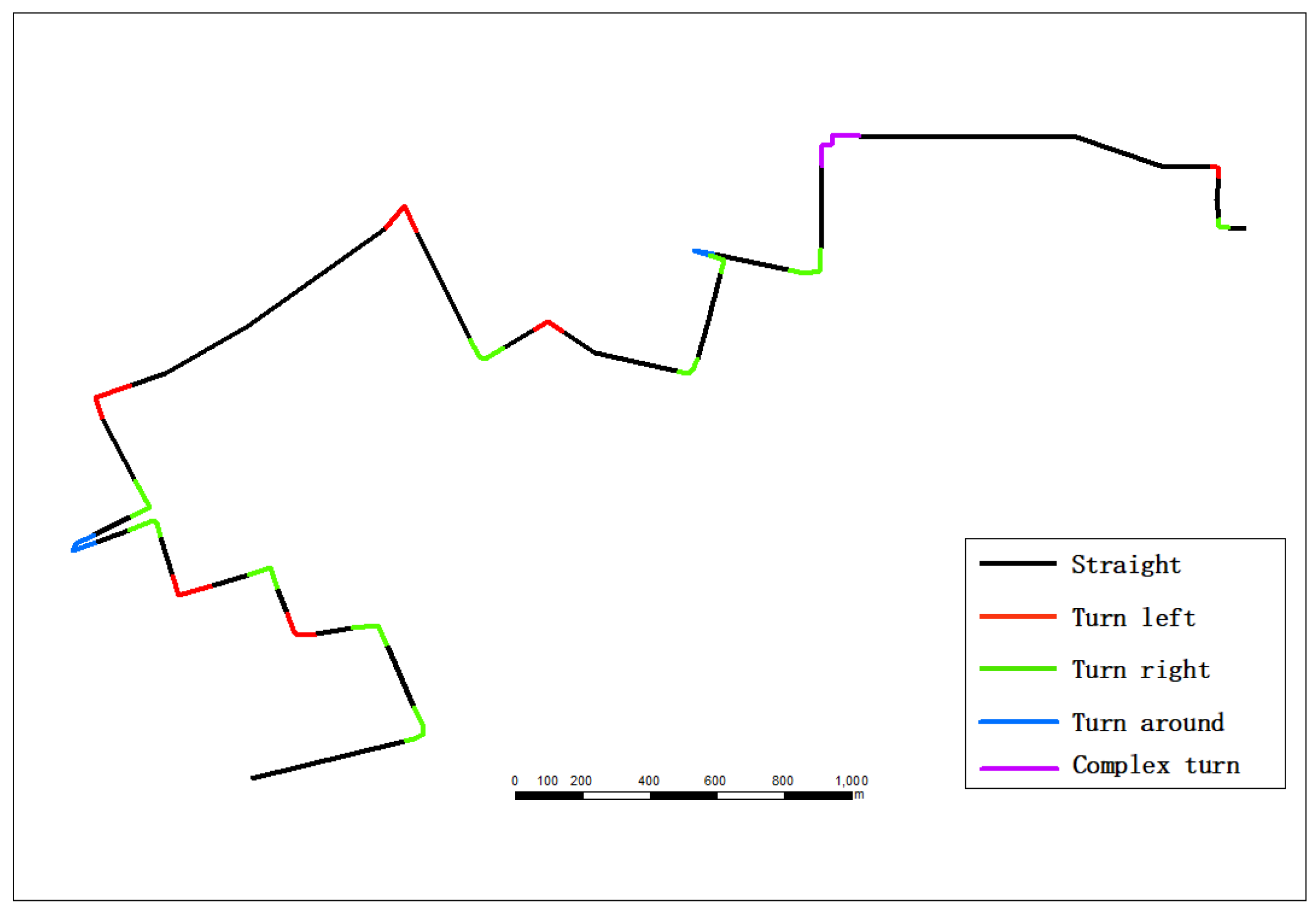
The navigation information of the whole trajectory can be generated according to the recognition result of the turning modes, with the compressed trajectory taken as the navigation route. Figure 15 presents the navigation messages for each part of the original trajectory. Navigation guidance will be provided twice: when the cyclist is 100 m away from the starting feature point of the turn, they will be prompted to turn 100 m ahead; when the cyclist is 10 m away from the starting feature point of the turn, they will be prompted to turn, and the specific turning mode will be given. In addition, when the cyclist deviates by more than 100 m from the navigation route, they will be informed of the deviation and they can check the navigation route map to correct the route in a timely manner. In order to verify the actual navigation effect, four volunteers with different mobile phone types were tested for four navigation routes. Table 7 reports the actual navigation results. All volunteers are able to correctly cycle along the navigation route and reach the destination via the navigation message. The average distance deviation between the actual cycling trajectory and navigation route is kept within 5 m.
5.4. Experiments in the Massive Cycling Trajectory Data
The massive quantities of experimental data come from the Sussex-Huawei Locomotion and Transportation (SHL) Dataset [30,31], from which we chose 50 reprehensive cycling trajectories. The total time of these trajectories is 19.14 h, the total distance is 596.3 km, and the total number of trajectory points is 68,277. Likewise, we use the proposed algorithm to extract turning feature points with the compression threshold set to 5 m. The extraction results are shown in Figure 16 below.
The extraction results are displayed on the electronic map platform, and we manually verified the correctness of this algorithm for turning mode identification. The recognition accuracy of the turning modes based only on the coordinate data is shown in Table 8, where we can see that over 99.2% of the turning modes can be correctly identified, the false identification rate is only about 12%, and omission identification is only about 0.8%. Generally speaking, the coordinate data collected by the position sensor can be used to correctly identify most of the turning modes, and the coordinate data have no requirement in terms of the posture of the mobile phone. However, when the satellite signal is weak, combining the coordinate data collected by the positioning sensor with azimuth data collected by the direction sensor positioning sensor can help to recognize the turning modes more accurately. To use the direction sensor, the phone needs to be fixed to the cycling vehicle.
6. Conclusions
In the current paper, we have proposed an algorithm that employs the positioning and direction sensors built in mobile smart phones to collect coordinate and azimuth data during cycling in order to identify trajectory turning modes. Navigation messages are then generated and shared with other users based on the identified turning modes, producing a cycling trajectory-based sharing navigation framework that is independent of road network data support. Experimental results reveal the ability of the algorithm to realize route navigation by analyzing the original trajectory, without requiring the support of road network data. Thus, the proposed framework is independent of electronic map platforms. Moreover, the algorithm combines the positioning and direction sensors to improve the robustness, and considers the interference from numerous real-life situations in the cycling trajectory collection (e.g., encountering traffic lights, cycling under overpasses or tall buildings, avoiding obstacles, etc.). This ensures the accurate extraction of turning modes. Finally, the algorithm classifies common turn modes as well as several complex turn modes, providing users with correct route guidance, even for complicated traffic conditions. In summary, the proposed algorithm can realize cycling route navigation for users based on just the provider’s cycling trajectory, without the need for road network data. This is suitable for cycling trajectory applications on mobile phones.
Author Contributions
Project administration, Lianhai Cao; supervision, Dongbao Zhao; writing—original draft, Kaixuan Zhang; writing—review and editing, Linlin Feng. All authors have read and agreed to the published version of the manuscript.
Funding
This work was partially funded by National Natural Science Foundation of China (No. 41971346), State Key Laboratory of Geo-Information Engineering (No. SKLGIE2020-M-4-1), and Natural Resources Research Projects of Henan Province (No. 2020--165--10).
Data Availability Statement
Publicly available datasets were analyzed in this study. This data can be found here: http://www.shl-dataset.org/download/.
Conflicts of Interest
The authors declare no conflict of interest.
References
- Dijkstra, E.W. A note on two problems in connexion with graphs. Numer. Math. 1959, 1, 269–271. [Google Scholar] [CrossRef] [Green Version]
- Bellman, R.E. On rounting problem. Q. Appl. Math. 1958, 16, 87–90. [Google Scholar] [CrossRef] [Green Version]
- Hart, E.P.; Nilsson, N.J.; Raphael, B. A formal basis for the heuristic determination of minimum cost paths. IEEE Trans. Syst. Sci. Cybern. 1968, 4, 100–107. [Google Scholar] [CrossRef]
- Jagadeesh, G.R.; Srikanthan, T.; Quek, K.H. Heuristic techniques for accelerating hierarchical routing on road networks. IEEE Trans. Intell. Transp. Syst. 2002, 3, 301–309. [Google Scholar] [CrossRef]
- Geisberger, R.; Sanders, P.; Schultes, D.; Delling, D. Contraction Hierarchies: Faster and simpler hierarchical routing in road networks. In Proceedings of the 7th International Workshop on Experimental Algorithms, Provincetown, MA, USA, 30 May–1 June 2008; pp. 319–333. [Google Scholar]
- Rajagopalan, R.; Mehrotra, K.G.; Mohan, C.K.; Vershney, P.K. Hierarchical path computation approach for large graphs. IEEE Trans. Aerosp. Electron. Syst. 2008, 44, 427–440. [Google Scholar] [CrossRef]
- Song, Q.; Li, M.; Li, X. Accurate and fast path computation on large urban road networks: A general approach. PLoS ONE 2018, 13, e0192274. [Google Scholar] [CrossRef]
- Wen, F.; Wang, X.; Zhang, G. Evolutionary-based automatic clustering method for optimizing multilevel network. Clust. Comput. 2017, 20, 3161–3172. [Google Scholar] [CrossRef]
- Song, Q.; Li, M.; Li, X. Accurate and fast path computation in urban environments using region pruning strategies. In Proceedings of the 36th Chinese Control Conference (CCC), Dalian, China, 26–28 July 2017; pp. 2778–2783. [Google Scholar]
- Ardakani, M.K.; Tavana, M.A. Decremental Approach with the A* Algorithm for Speeding-up the Optimization Process in Dynamic Shortest Path Problems. Measurement 2015, 60, 299–307. [Google Scholar] [CrossRef]
- Tang, J.; Song, Y.; Miller, H.J.; Zhou, X. Estimating the most likely space–time paths, dwell times and path uncertainties from vehicle trajectory data: A time geographic method. Transp. Res. Part C Emerg. Technol. 2016, 66, 176–194. [Google Scholar] [CrossRef] [Green Version]
- Wang, Y.; Li, G.; Tang, N. Querying shortest paths on time dependent road networks. Proc. VLDB Endow. 2019, 12, 1249–1261. [Google Scholar] [CrossRef] [Green Version]
- Fa-mei, H.E.; Yi-na, X.U.; Xu-ren, W.; Meng-bo, X.; Zi-han, X. An Improved Ant Colony Algorithm for Solving Time-Dependent Road Network Path Planning Problem. In Proceedings of the 6th International Conference on Information Science and Control Engineering (ICISCE), Shanghai, China, 20–22 December 2019; pp. 126–130. [Google Scholar]
- He, F.; Xu, Y.; Wang, X.; Feng, A. ALT-Based Route Planning in Dynamic Time-Dependent Road Networks. In Proceedings of the 2nd International Conference on Machine Learning and Machine Intelligence, Jakarta, Indonesia, 18 September 2019; pp. 35–39. [Google Scholar]
- Sheng, Y.; Mei, X. Uncertain random shortest path problem. Soft Comput. 2020, 24, 2431–2440. [Google Scholar] [CrossRef]
- Prakash, A.A. Pruning algorithm for the least expected travel time path on stochastic and time-dependent networks. Transp. Res. Part B Methodol. 2018, 108, 127–147. [Google Scholar] [CrossRef]
- Chen, P.; Tong, R.; Yu, B.; Wang, Y. Reliable shortest path finding in stochastic time-dependent road network with spatial-temporal link correlations: A case study from Beijing. Expert Syst. Appl. 2020, 147, 113192. [Google Scholar] [CrossRef]
- Filipovska, M.; Mahmassani, H.S. Reliable Least-Time Path Estimation and Computation in Stochastic Time-Varying Networks with Spatio-Temporal Dependencies. In Proceedings of the IEEE 23rd International Conference on Intelligent Transportation Systems (ITSC), Rhodes, Greece, 20–23 September 2020; pp. 1–6. [Google Scholar]
- Zhao, D.; Stefanakis, E. Mining massive taxi trajectories for rapid fastest path planning in dynamic multi-level landmark network. Comput. Environ. Urban Syst. 2018, 72, 221–231. [Google Scholar] [CrossRef]
- Yuan, J.; Zheng, Y.; Xie, X.; Sun, G. T-Drive: Enhancing Driving Directions with Taxi Drivers Intelligence. IEEE Trans. Knowl. Data Eng. 2013, 25, 220–232. [Google Scholar] [CrossRef]
- Yang, L.; Kwan, M.P.; Pan, X.; Wan, B.; Zhou, S. Scalable space-time trajectory cube for path-finding: A study using big taxi trajectory data. Transp. Res. Part B Methodol. 2017, 101, 1–27. [Google Scholar] [CrossRef]
- He, Z.; Chen, K.; Chen, X. A collaborative method for route discovery using taxi drivers’ experience and preferences. IEEE Trans. Intell. Transp. Syst. 2017, 19, 2505–2514. [Google Scholar] [CrossRef]
- Li, Y.; Su, H.; Demiryurek, U.; Zheng, B.; He, T.; Shahabi, C. Pare: A system for personalized route guidance. In Proceedings of the 26th International Conference on World Wide Web, Perth, Australia, 3–7 April 2017; pp. 637–646. [Google Scholar]
- Su, H.; Cong, G.; Chen, W.; Su, Q.; Zheng, B.; Zheng, K. PerRD: A System for Personalized Route Description. In Proceedings of the IEEE 35th International Conference on Data Engineering (ICDE), Macau, China, 8–11 April 2019; pp. 1658–1661. [Google Scholar]
- Zhang, H.; Huangfu, W.; Hu, X. Inferring the Most Popular Route Based on Ant Colony Optimization with Trajectory Data. In Wireless Sensor Networks; Springer: Singapore, 2017; pp. 307–318. [Google Scholar]
- Ceikute, V.; Jensen, C.S. Vehicle routing with user-generated trajectory data. In Proceedings of the 16th IEEE International Conference on Mobile Data Management, Pittsburgh, PA, USA, 15–18 June 2015; pp. 14–23. [Google Scholar]
- Lim, K.H.; Chan, J.; Leckie, C.; Karunasekera, S. Personalized trip recommendation for tourists based on user interests, points of interest visit durations and visit recency. Knowl. Inf. Syst. 2018, 54, 375–406. [Google Scholar] [CrossRef]
- Ge, C. Personalized travel route recommendation using collaborative filtering based on GPS trajectories. Int. J. Digit. Earth 2018, 11, 1–24. [Google Scholar]
- Quercia, D.; Schifanella, R.; Aiello, L.M. The Shortest Path to Happiness: Recommending Beautiful, Quiet, and Happy Routes in the City. In Proceedings of the ACM Hypertext, Santiago, Chile, 1–4 September 2014. [Google Scholar]
- Gjoreski, H.; Ciliberto, M.; Wang, L.; Morales, F.; Mekki, S.; Valentin, S.; Roggen, D. The University of Sussex-Huawei locomotion and transportation dataset for multimodal analytics with mobile devices. IEEE Access 2018, 6, 42592–42604. [Google Scholar] [CrossRef]
- Wang, L.; Gjoreski, H.; Ciliberto, M.; Mekki, S.; Valentin, S.; Roggen, D. Enabling reproducible research in sensor-based transportation mode recognition with the Sussex-Huawei dataset. IEEE Access 2019, 7, 10870–10891. [Google Scholar] [CrossRef]
Figure 1.
Diagram of cycling trajectory-based navigation.

Figure 2.
Mobile phone three-axis coordinate system.

Figure 3.
Change of the three-axis data of the direction sensor during the process of turning: (a) a 20° left turn; (b) a right 90° turn; (c) a 180° turn.
Figure 3.
Change of the three-axis data of the direction sensor during the process of turning: (a) a 20° left turn; (b) a right 90° turn; (c) a 180° turn.

Figure 4.
The recognition of turn sequences.

Figure 5.
Diagram of determination of turning modes: (a) turning feature points of left turn; (b) azimuth angle change of the direction sensor.
Figure 5.
Diagram of determination of turning modes: (a) turning feature points of left turn; (b) azimuth angle change of the direction sensor.

Figure 6.
Diagram of turning at different road intersections: (a) turns at Y-shaped road intersection; (b) turns at cross-shaped road intersection.
Figure 6.
Diagram of turning at different road intersections: (a) turns at Y-shaped road intersection; (b) turns at cross-shaped road intersection.

Figure 7.
Diagram of small curves in cycling trajectory: (a) changing lanes; (b) avoiding obstacles.
Figure 7.
Diagram of small curves in cycling trajectory: (a) changing lanes; (b) avoiding obstacles.

Figure 8.
Diagram of complex turning mode: (a) complex turning mode in narrow road; (b) complex turning mode in circular road; (c) complex turning mode at large road intersection.
Figure 8.
Diagram of complex turning mode: (a) complex turning mode in narrow road; (b) complex turning mode in circular road; (c) complex turning mode at large road intersection.

Figure 9.
The first example of cycling trajectory.

Figure 10.
The second example of cycling trajectory.

Figure 11.
The third example of cycling trajectory.

Figure 12.
The fourth example of cycling trajectory.

Figure 13.
The extraction results of turning feature points under the 5m compression threshold: (a) the first example of cycling trajectory; (b) the second example of cycling trajectory; (c) the third example of cycling trajectory; (d) the fourth example of cycling trajectory.
Figure 13.
The extraction results of turning feature points under the 5m compression threshold: (a) the first example of cycling trajectory; (b) the second example of cycling trajectory; (c) the third example of cycling trajectory; (d) the fourth example of cycling trajectory.

Figure 14.
Overlay of trajectory data and actual road network.

Figure 15.
Navigation information generated by this algorithm.

Figure 16.
The extraction results of turning feature points under the 5 m compression threshold.


Table 1.
Extraction results of Turning feature points under different compression thresholds.
| Trajectory Number | Number of Original Trajectory Points | Number of Feature Points under 3 m Compression Threshold | Number of Feature Points under 5 m Compression Threshold | Number of Feature Points under 7 m Compression Threshold | Number of Feature Points under 10 m Compression Threshold |
|---|---|---|---|---|---|
| 1 | 2187 | 59 | 39 | 31 | 28 |
| 2 | 1682 | 56 | 41 | 36 | 28 |
| 3 | 2691 | 75 | 48 | 40 | 28 |
| 4 | 1690 | 53 | 34 | 29 | 23 |
Table 2.
Recognition accuracy of turning modes when the compression threshold is set to 3 m.
| Trajectory Number | Actual Number of Turns | Only Relying on Coordinate Data to Identify Turning Modes | Coordinate Data Are Combined with Direction Sensors to Identify Turning Modes | ||||
|---|---|---|---|---|---|---|---|
| Correct Identification Number | Number of False Identifications | Number of Omissions Identified | Correct Identification Number | Number of False Identifications | Number of Omissions Identified | ||
| 1 | 19 | 19 | 0 | 0 | 19 | 0 | 0 |
| 2 | 16 | 14 | 5 | 2 | 14 | 2 | 2 |
| 3 | 19 | 18 | 3 | 1 | 18 | 0 | 1 |
| 4 | 11 | 11 | 2 | 0 | 11 | 0 | 0 |
Table 3.
Recognition accuracy of turning modes when the compression threshold is set to 5 m.
| Trajectory Number | Actual Number of Turns | Only Relying on Coordinate Data to Identify Turning Modes | Coordinate Data Are Combined with Direction Sensors to Identify Turning Modes | ||||
|---|---|---|---|---|---|---|---|
| Correct Identification Number | Number of False Identifications | Number of Omissions Identified | Correct Identification Number | Number of False Identifications | Number of Omissions Identified | ||
| 1 | 19 | 19 | 0 | 0 | 19 | 0 | 0 |
| 2 | 16 | 16 | 1 | 0 | 16 | 0 | 0 |
| 3 | 19 | 19 | 0 | 0 | 19 | 0 | 0 |
| 4 | 11 | 11 | 2 | 0 | 11 | 0 | 0 |
Table 4.
Recognition accuracy of turning modes when the compression threshold is set to 7 m.
| Trajectory Number | Actual Number of Turns | Only Relying on Coordinate Data to Identify Turning Modes | Coordinate Data Are Combined with Direction Sensors to Identify Turning Modes | ||||
|---|---|---|---|---|---|---|---|
| Correct Identification Number | Number of False Identifications | Number of Omissions Identified | Correct Identification Number | Number of False Identifications | Number of Omissions Identified | ||
| 1 | 19 | 19 | 0 | 0 | 19 | 0 | 0 |
| 2 | 16 | 16 | 1 | 0 | 16 | 0 | 0 |
| 3 | 19 | 19 | 0 | 0 | 19 | 0 | 0 |
| 4 | 11 | 11 | 2 | 0 | 11 | 0 | 0 |
Table 5.
Recognition accuracy of turning modes when the compression threshold is set to 10 m.
| Trajectory Number | Actual Number of Turns | Only Relying on Coordinate Data to Identify Turning Modes | Coordinate Data Are Combined with Direction Sensors to Identify Turning Modes | ||||
|---|---|---|---|---|---|---|---|
| Correct Identification Number | Number of False Identifications | Number of Omissions Identified | Correct Identification Number | Number of False Identifications | Number of Omissions Identified | ||
| 1 | 19 | 19 | 0 | 0 | 19 | 0 | 0 |
| 2 | 16 | 14 | 0 | 2 | 14 | 0 | 2 |
| 3 | 19 | 19 | 0 | 0 | 19 | 0 | 0 |
| 4 | 11 | 11 | 2 | 0 | 11 | 0 | 0 |
Table 6.
Turning modes recognized by this algorithm.
| Actual Turn Mode | Turn Mode Recognized by This Algorithm | ID of Start Point of Turn | ID of End Point of Turn | Longitude of Start Point of Turn | Latitude of Start Point of Turn | Longitude of End Point of Turn | Latitude of End Point of Turn |
|---|---|---|---|---|---|---|---|
| Turn right | Turn right | 1 | 1 | 113.787678 | 34.786924 | 113.787678 | 34.786924 |
| Turn left | Turn left | 2 | 2 | 113.787665 | 34.788497 | 113.787665 | 34.788497 |
| Turn left | Complex turning mode | 5 | 7 | 113.777291 | 34.78937 | 113.777039 | 34.789087 |
| Turn right | Turn right | 8 | 8 | 113.776993 | 34.785729 | 113.776993 | 34.785729 |
| Turn around | Turn around | 10 | 10 | 113.773606 | 34.786285 | 113.773606 | 34.786285 |
| Turn right | Turn right | 11 | 11 | 113.774441 | 34.78602 | 113.774441 | 34.78602 |
| Turn right | Turn right | 13 | 14 | 113.773575 | 34.783068 | 113.773442 | 34.782966 |
| Turn left | Turn left | 16 | 16 | 113.769701 | 34.784371 | 113.769701 | 34.784371 |
| Turn right | Turn right | 17 | 18 | 113.768032 | 34.783375 | 113.767847 | 34.783414 |
| Turn left | Turn left | 19 | 19 | 113.765872 | 34.78751 | 113.765872 | 34.78751 |
| Turn left | Turn left | 23 | 23 | 113.757566 | 34.782305 | 113.757566 | 34.782305 |
| Turn right | Turn right | 25 | 25 | 113.759036 | 34.779385 | 113.759036 | 34.779385 |
| Turn around | Turn around | 26 | 26 | 113.75691 | 34.778221 | 113.75691 | 34.778221 |
| Turn right | Turn right | 27 | 28 | 113.759128 | 34.779042 | 113.759218 | 34.778979 |
| Turn left | Turn left | 29 | 29 | 113.759825 | 34.777004 | 113.759825 | 34.777004 |
| Turn right | Turn right | 30 | 30 | 113.762244 | 34.777771 | 113.762244 | 34.777771 |
| Turn left | Turn left | 32 | 33 | 113.762868 | 34.776074 | 113.762868 | 34.776074 |
| Turn right | Turn right | 34 | 34 | 113.765143 | 34.776204 | 113.765143 | 34.776204 |
| Turn right | Turn right | 35 | 37 | 113.766377 | 34.773492 | 113.766132 | 34.773175 |
Table 7.
Deviation between actual cycling trajectory of volunteers and navigation route.
| Trajectory Number | Maximum Deviation Distance between Actual Cycling Trajectory of Volunteers and Navigation Route (Meters) | Average Deviation Distance between Actual Cycling Trajectory of Volunteers and Navigation Route (Meters) | Time Consumption (Minutes) |
|---|---|---|---|
| 1 | 23.5 | 3.85 | 31 |
| 2 | 25.8 | 4.30 | 36 |
| 3 | 26.9 | 5.75 | 39 |
| 4 | 19.2 | 4.55 | 30 |
Table 8.
Recognition accuracy of turning modes when the compression threshold is set to 5 m.
| Turn Mode | Actual Number of Turns | Correct Identification Number | Number of False Identifications | Number of Omissions Identified |
|---|---|---|---|---|
| Turn left | 382 | 378 | 20 | 4 |
| Turn right | 329 | 329 | 30 | 0 |
| Turn around | 17 | 15 | 6 | 2 |
| Complex turning mode | 20 | 20 | 34 | 0 |
Publisher’s Note: MDPI stays neutral with regard to jurisdictional claims in published maps and institutional affiliations. |
© 2021 by the authors. Licensee MDPI, Basel, Switzerland. This article is an open access article distributed under the terms and conditions of the Creative Commons Attribution (CC BY) license (https://creativecommons.org/licenses/by/4.0/).
Share and Cite
MDPI and ACS Style
Zhang, K.; Zhao, D.; Feng, L.; Cao, L. Cycling Trajectory-Based Navigation Independent of Road Network Data Support. ISPRS Int. J. Geo-Inf. 2021, 10, 398. https://0-doi-org.brum.beds.ac.uk/10.3390/ijgi10060398
AMA Style
Zhang K, Zhao D, Feng L, Cao L. Cycling Trajectory-Based Navigation Independent of Road Network Data Support. ISPRS International Journal of Geo-Information. 2021; 10(6):398. https://0-doi-org.brum.beds.ac.uk/10.3390/ijgi10060398
Chicago/Turabian StyleZhang, Kaixuan, Dongbao Zhao, Linlin Feng, and Lianhai Cao. 2021. "Cycling Trajectory-Based Navigation Independent of Road Network Data Support" ISPRS International Journal of Geo-Information 10, no. 6: 398. https://0-doi-org.brum.beds.ac.uk/10.3390/ijgi10060398
Note that from the first issue of 2016, this journal uses article numbers instead of page numbers. See further details here.