
A Trajectory Scoring Tool for Local Anomaly Detection in Maritime Traffic Using Visual Analytics


Abstract
:1. Introduction
- Is it possible to identify local anomalies using one or a combination of features given a port of origin and a port of destination?
- Is it possible to make sense of the interpolation and the uncertainty it may cause when determining anomalies?
2. Background
2.1. Automatic Identification System (AIS)
2.2. Anomaly Detection
2.2.1. Types of Anomalies
2.2.2. Anomaly Detection by Vessel Type
2.3. Spatial Region, Trajectory, and Subtrajectory
2.4. Global and Local Anomaly Detection
2.5. Visual Analytics
3. Related Work
3.1. Automated Anomaly Detection of Vessel Trajectories
3.2. Visual Anomaly Detection of Trajectories in Maritime Traffic
4. Methods
4.1. Requirements
- The tool should support the identification of trips that may have anomalous behavior.
- The tool should support the identification of local anomalies.
- The tool should improve the user’s understanding of where interpolation has happened in a trajectory and its impact, if any, on anomalies.
- The tool should support some explanation of the cause of the anomaly.
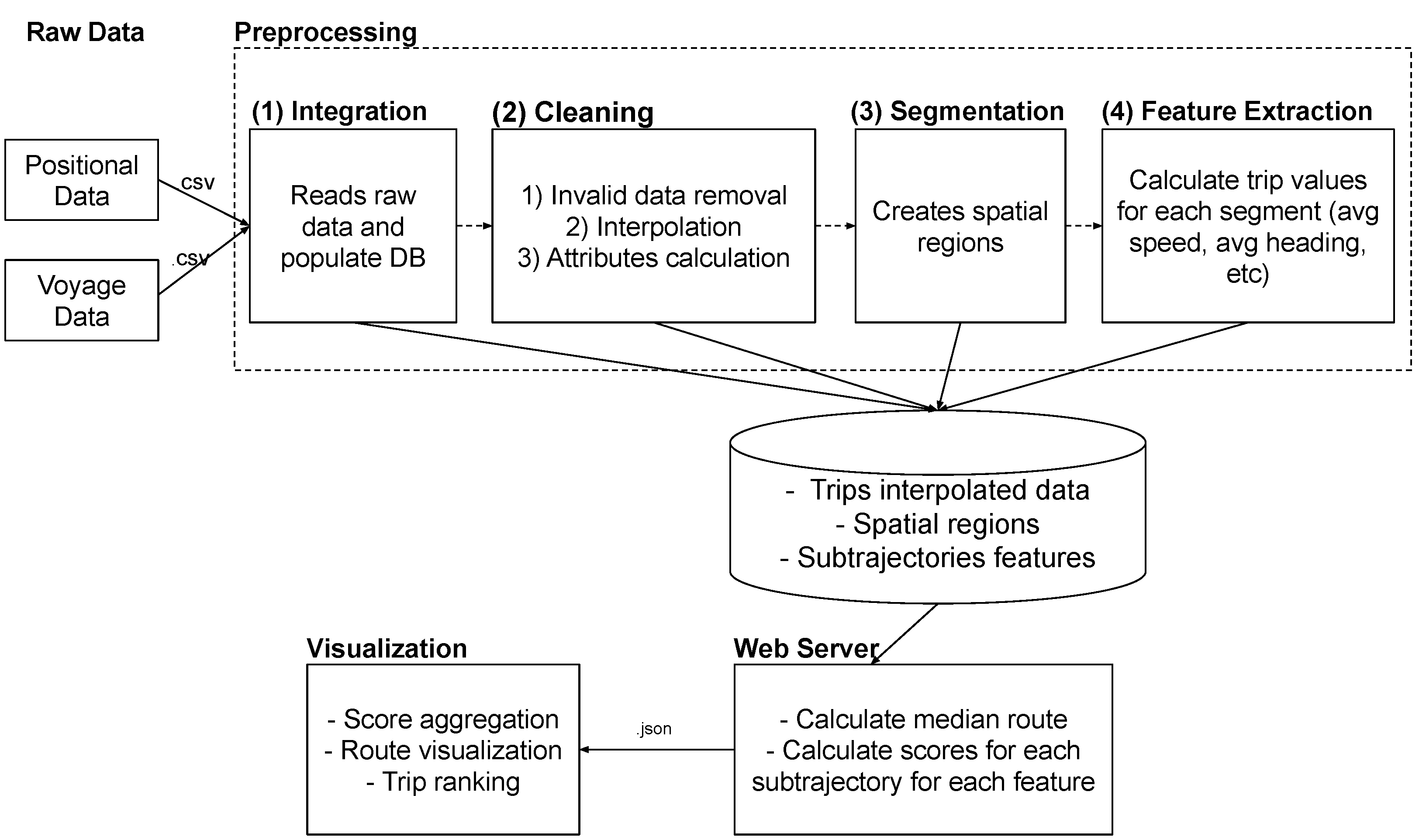
4.2. Framework Overview
4.3. Tool Rationale
4.3.1. Why Use Spatial Regions?
4.3.2. Why Use Mean and Scores?
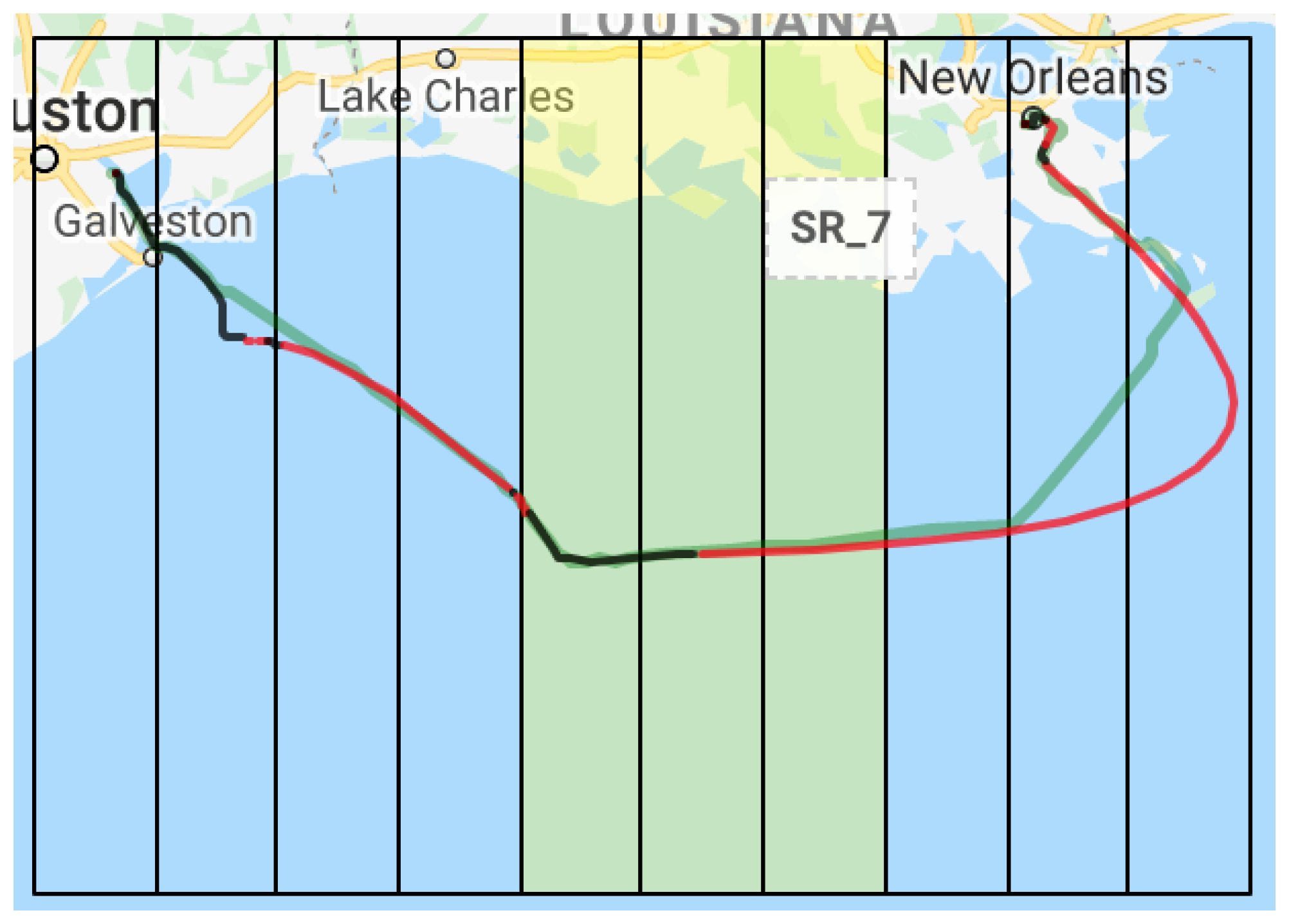
4.3.3. Why Show a Map?
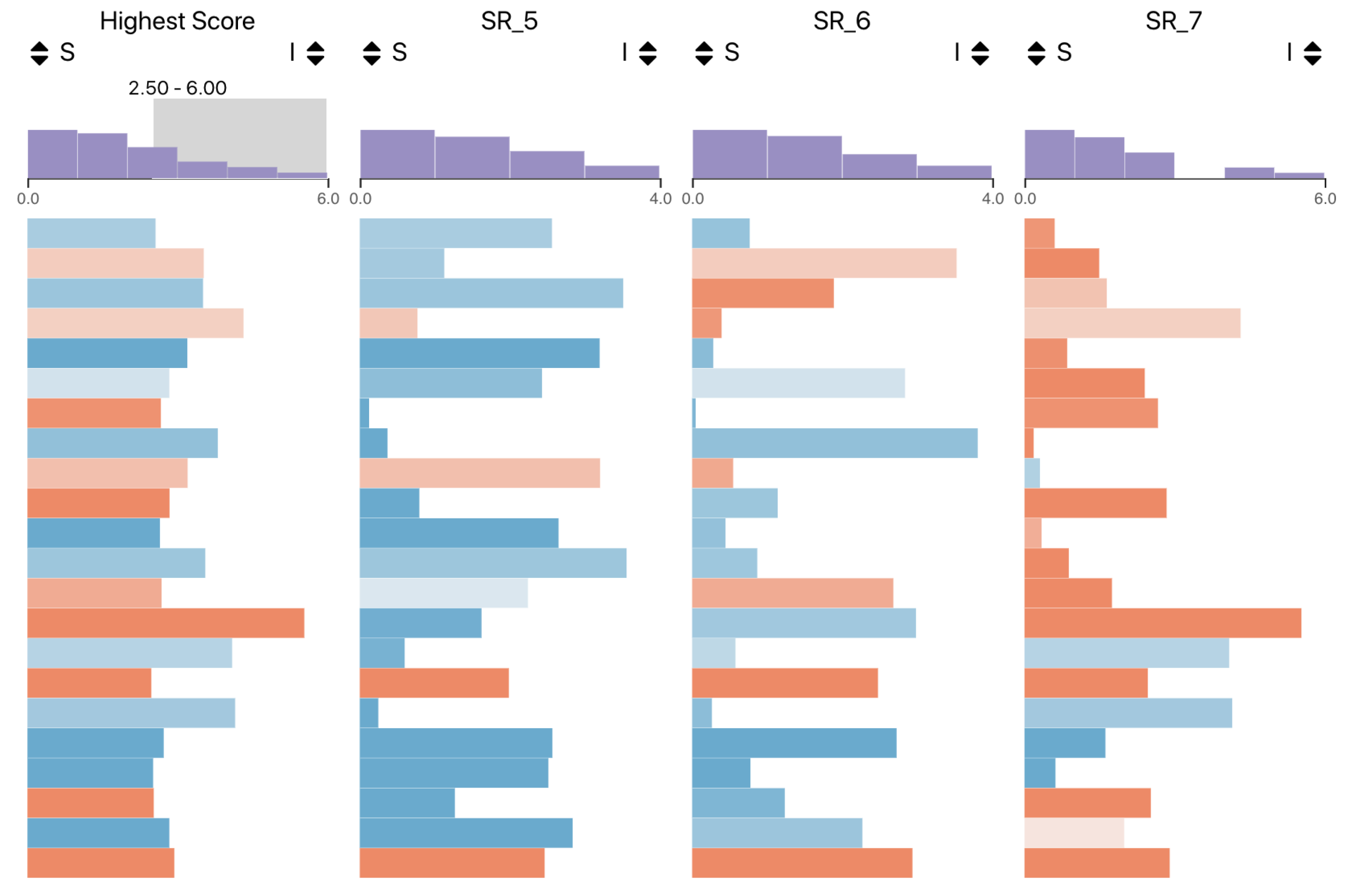
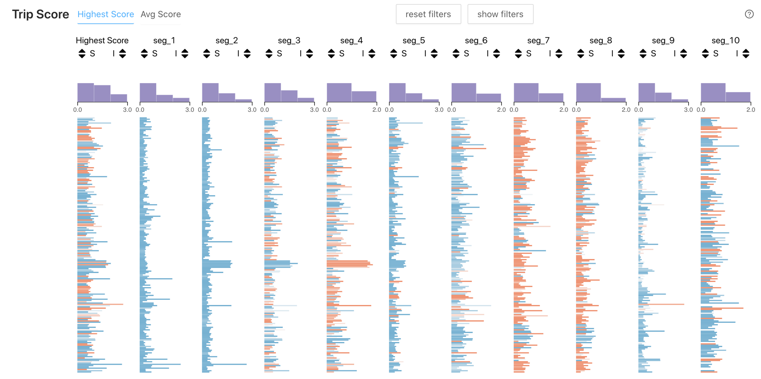
4.3.4. Why Show Scores in a Table-Like Visualization?
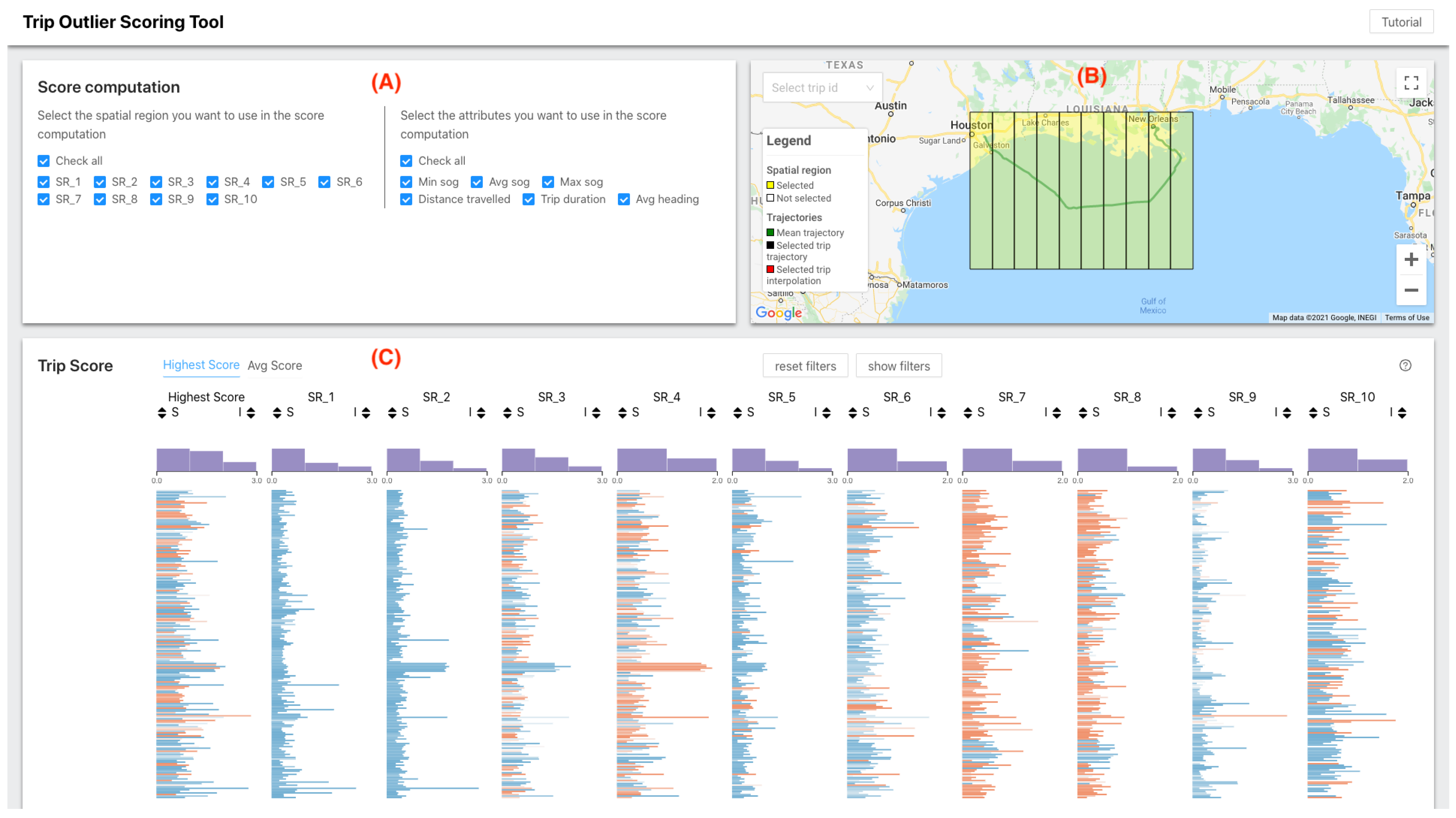
4.4. Trip Outlier Scoring Tool (TOST)
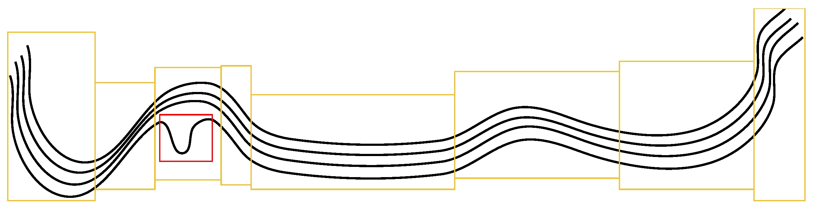
4.4.1. Data Interpolation
4.4.2. Subtrajectory Attributes
4.4.3. Subtrajectory Score
5. A Use Case
6. Tests with Users
6.1. Experimental Setup
6.2. Scenarios
6.3. User Test Questions
- How many trips are outliers?Our idea with this question was to validate whether the participants could identify which trips were outliers. They would have to filter the data either by brushing or typing directly into the filter component. Since asking for several IDs can be time-consuming and prone to errors, we asked for the number of trips that were outliers.
- What is the identifier of the trip with the highest score?In this question, we tried to see if the participants understood both how to sort trips and the ranking concept to find the trajectory that was the most anomalous in a given scenario.
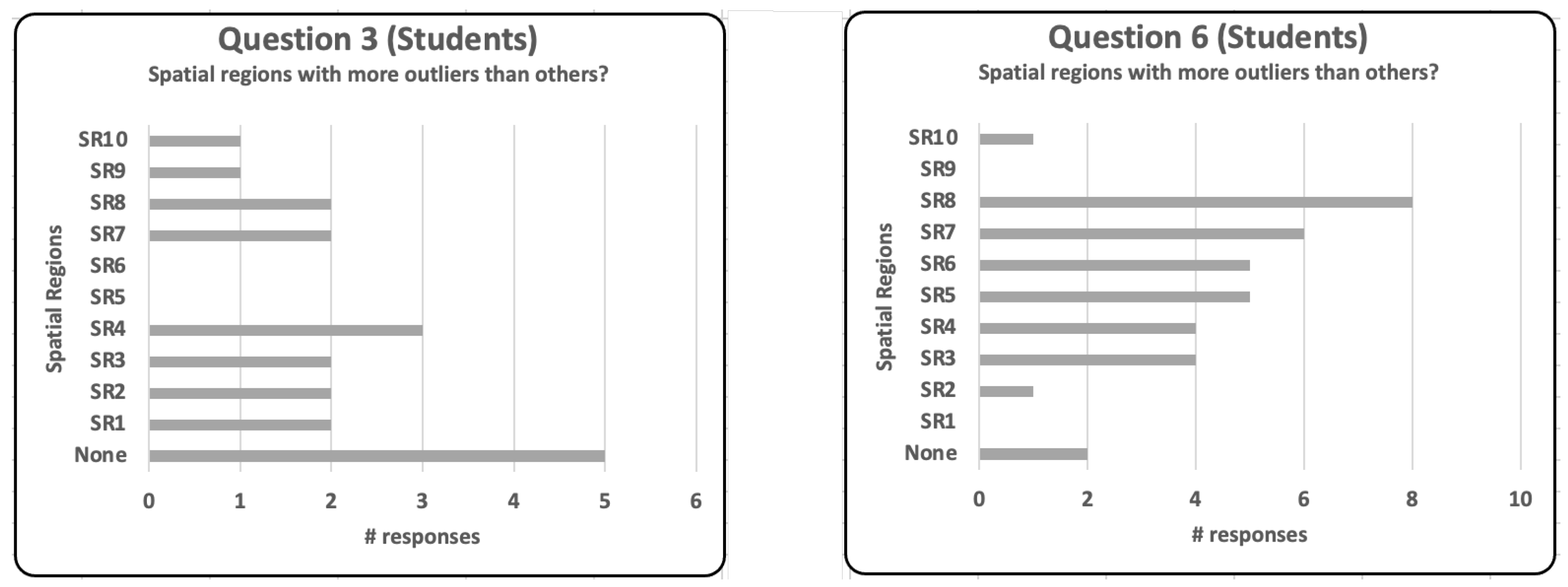
- Which spatial regions have more outliers than others?The purpose of this question was to check whether the participants could use the score distribution plots to identify and visualize spatial regions with a higher number of anomalies.
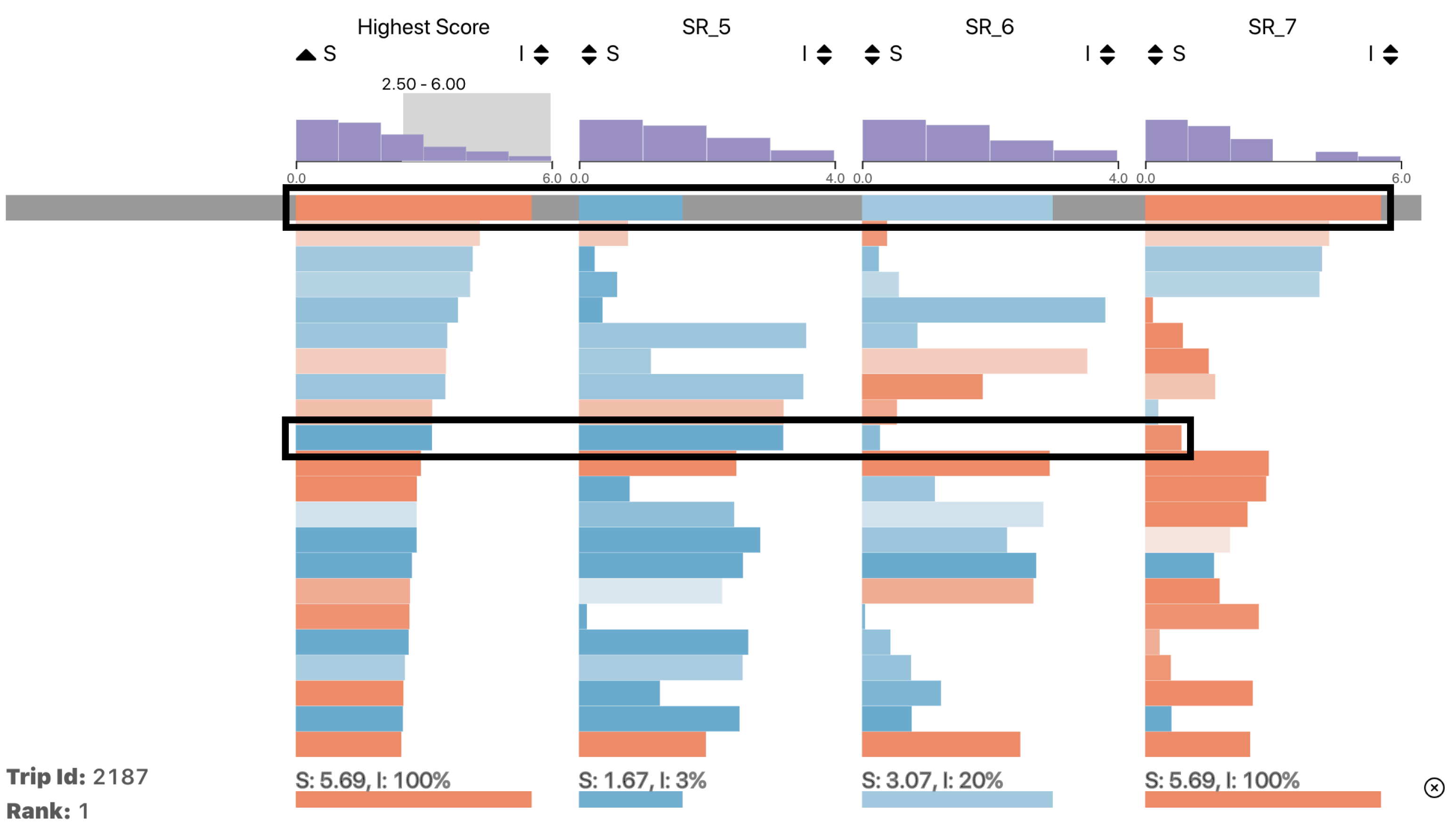
- In which spatial regions did trip X have an outlier behavior?In this question, we wanted to see if the participants understood the score concept and how to visualize it, either by hovering over a row and seeing the score at the bottom of the table or by looking at the axis at the top of the table.
- How much interpolation do you think there is in this scenario?Ideally, we would like to see the data set with few interpolations. Based on this information, and without using any type of sorting, how much interpolation do you think there is in this data set? This question tries to assess if using color to interpret the interpolation gives an overall idea of the amount of interpolation used in the data set.
- How many trips have, on average, above 50% interpolation?This question tries to verify if the participant understood how the interpolation concept is displayed and if they are able to find the number of trajectories for which there is not enough information to label it as anomalous.
- For a given trip in a scenario, choose the most appropriate option.In this question, we put together the concepts of score, interpolation, and trajectory together. The user then had to choose one of the following options:
- -
- It is not an outlier; it has a good score and good interpolation.
- -
- It is an outlier; it has a bad score and bad interpolation.
- -
- I can’t say, there is too much interpolation, or the interpolation seems incorrect.
6.4. Results
7. Conclusions and Limitations
Author Contributions
Funding
Data Availability Statement
Conflicts of Interest
References
- Pallotta, G.; Vespe, M.; Bryan, K. Vessel pattern knowledge discovery from AIS data: A framework for anomaly detection and route prediction. Entropy 2013, 15, 2218–2245. [Google Scholar] [CrossRef] [Green Version]
- Sheng, P.; Yin, J. Extracting shipping route patterns by trajectory clustering model based on automatic identification system data. Sustainability 2018, 10, 2327. [Google Scholar] [CrossRef] [Green Version]
- Zhen, R.; Jin, Y.; Hu, Q.; Shao, Z.; Nikitakos, N. Maritime anomaly detection within coastal waters based on vessel trajectory clustering and Naïve Bayes Classifier. J. Navig. 2017, 70, 648. [Google Scholar] [CrossRef]
- Zissis, D.; Xidias, E.K.; Lekkas, D. A cloud based architecture capable of perceiving and predicting multiple vessel behaviour. Appl. Soft Comput. 2015, 35, 652–661. [Google Scholar] [CrossRef] [Green Version]
- Fiorini, M.; Capata, A.; Bloisi, D.D. AIS data visualization for maritime spatial planning (MSP). Int. J. e-Navig. Marit. Econ. 2016, 5, 45–60. [Google Scholar] [CrossRef]
- Dividino, R.; Soares, A.; Matwin, S.; Isenor, A.W.; Webb, S.; Brousseau, M. Semantic integration of real-time heterogeneous data streams for ocean-related decision making. In Big Data and Artificial Intelligence for Military Decision Making; The Science and Technology Organization-STO: Brussels, Belgium, 2018. [Google Scholar] [CrossRef]
- Soares, A.; Dividino, R.; Abreu, F.; Brousseau, M.; Isenor, A.W.; Webb, S.; Matwin, S. CRISIS: Integrating AIS and ocean data streams using semantic web standards for event detection. In Proceedings of the 2019 International Conference on Military Communications and Information Systems (ICMCIS), Budva, Montenegro, 14–15 May 2019; pp. 1–7. [Google Scholar]
- Mascaro, S.; Nicholso, A.E.; Korb, K.B. Anomaly detection in vessel tracks using Bayesian networks. Int. J. Approx. Reason. 2014, 55, 84–98. [Google Scholar] [CrossRef]
- Roy, J. Anomaly detection in the maritime domain. Optics and Photonics in Global Homeland Security IV. Int. Soc. Opt. Photonics 2008, 6945, 69450W. [Google Scholar]
- Lavigne, V. Interactive visualization applications for maritime anomaly detection and analysis. In ACM SIGKDD Workshop on Interactive Data Exploration and Analytics; Association for Computing Machinery: New York, NY, USA, 2014; p. 75. [Google Scholar]
- d’Afflisio, E.; Braca, P.; Millefiori, L.M.; Willett, P. Detecting anomalous deviations from standard maritime routes using the Ornstein–Uhlenbeck process. IEEE Trans. Signal Process. 2018, 66, 6474–6487. [Google Scholar] [CrossRef] [Green Version]
- Varlamis, I.; Tserpes, K.; Etemad, M.; Júnior, A.S.; Matwin, S. A Network Abstraction of Multi-vessel Trajectory Data for Detecting Anomalies; EDBT/ICDT Workshops: Lisbon, Portugal, 2019. [Google Scholar]
- Varlamis, I.; Kontopoulos, I.; Tserpes, K.; Etemad, M.; Soares, A.; Matwin, S. Building navigation networks from multi-vessel trajectory data. GeoInformatica 2021, 25, 69–97. [Google Scholar] [CrossRef]
- Laxhammar, R. Anomaly Detection in Trajectory Data for Surveillance Applications. Ph.D. Thesis, Örebro Universitet, Örebro, Sweden, 2011. [Google Scholar]
- Willems, N.; Van De Wetering, H.; Van Wijk, J.J. Visualization of vessel movements. In Computer Graphics Forum; Wiley Online Library: Hoboken, NJ, USA, 2009; Volume 28, pp. 959–966. [Google Scholar]
- Martineau, E.; Roy, J. Maritime Anomaly Detection: Domain Introduction and Review of Selected Literature; Defence Research and Development Canada: Quebec, QC, Canada, 2011. [Google Scholar]
- Riveiro, M.; Falkman, G.; Ziemke, T.; Warston, H. VISAD: An interactive and visual analytical tool for the detection of behavioral anomalies in maritime traffic data. In Proceedings of the SPIE Defense, Security, and Sensing, Orlando, FL, USA, 13–17 April 2009. [Google Scholar]
- Riveiro, M.; Falkman, G. The role of visualization and interaction in maritime anomaly detection. In Proceedings of the IS&T/SPIE Electronic Imaging, San Francisco, CA, USA, 23–27 January 2011; Volume 7868, p. 78680M. [Google Scholar]
- Riveiro, M.; Falkman, G.; Ziemke, T. Improving maritime anomaly detection and situation awareness through interactive visualization. In Proceedings of the 2008 11th International Conference on Information Fusion, Cologne, Germany, 30 June–3 July 2008; pp. 1–8. [Google Scholar]
- May Petry, L.; Soares, A.; Bogorny, V.; Brandoli, B.; Matwin, S. Challenges in Vessel Behavior and Anomaly Detection: From Classical Machine Learning to Deep Learning. In Advances in Artificial Intelligence; Springer International Publishing: Cham, Switzerland, 2020; pp. 401–407. [Google Scholar]
- Dimitrova, T.; Tsois, A.; Camossi, E. Development of a web-based geographical information system for interactive visualization and analysis of container itineraries. Int. J. Comput. Inf. Technol 2014, 3, 1–8. [Google Scholar]
- Yang, W.; Gao, Y.; Cao, L. TRASMIL: A local anomaly detection framework based on trajectory segmentation and multi-instance learning. Comput. Vis. Image Underst. 2013, 117, 1273–1286. [Google Scholar] [CrossRef]
- Júnior, A.S.; Renso, C.; Matwin, S. Analytic: An active learning system for trajectory classification. IEEE Comput. Graph. Appl. 2017, 37, 28–39. [Google Scholar] [CrossRef]
- Soares, A.; Rose, J.; Etemad, M.; Renso, C.; Matwin, S. VISTA: A Visual Analytics Platform for Semantic Annotation of Trajectories. In Proceedings of the EDBT: 22nd International Conference on Extending Database Technology, Lisbon, Portugal, 26–29 March 2019; pp. 570–573. [Google Scholar]
- Zhang, D.; Li, J.; Wu, Q.; Liu, X.; Chu, X.; He, W. Enhance the AIS data availability by screening and interpolation. In Proceedings of the 2017 4th International Conference on Transportation Information and Safety (ICTIS), Banff, AB, Canada, 8–10 August 2017; pp. 981–986. [Google Scholar]
- Nguyen, V.S.; Im, N.K.; Lee, S.M. The interpolation method for the missing AIS data of ship. J. Navig. Port Res. 2015, 39, 377–384. [Google Scholar] [CrossRef] [Green Version]
- Liu, C.; Chen, X. Inference of single vessel behaviour with incomplete satellite-based AIS data. J. Navig. 2013, 66, 813. [Google Scholar] [CrossRef] [Green Version]
- Mazzarella, F.; Vespe, M.; Alessandrini, A.; Tarchi, D.; Aulicino, G.; Vollero, A. A novel anomaly detection approach to identify intentional AIS on-off switching. Expert Syst. Appl. 2017, 78, 110–123. [Google Scholar] [CrossRef]
- Handayani, D.O.D.; Sediono, W.; Shah, A. Anomaly detection in vessel tracking using support vector machines (SVMs). In Proceedings of the 2013 International Conference on Advanced Computer Science Applications and Technologies, Kuching, Malaysia, 23–24 December 2013; pp. 213–217. [Google Scholar]
- Eriksen, T.; Høye, G.; Narheim, B.; Meland, B.J. Maritime traffic monitoring using a space-based AIS receiver. Acta Astronaut. 2006, 58, 537–549. [Google Scholar] [CrossRef]
- Wu, X.; Rahman, A.; Zaloom, V.A. Study of travel behavior of vessels in narrow waterways using AIS data—A case study in Sabine-Neches Waterways. Ocean. Eng. 2018, 147, 399–413. [Google Scholar] [CrossRef]
- Breunig, M.M.; Kriegel, H.P.; Ng, R.T.; Sander, J. LOF: Identifying density-based local outliers. In Proceedings of the 2000 ACM SIGMOD International Conference on Management of Data, Dallas, TX, USA, 15–18 May 2000; pp. 93–104. [Google Scholar]
- Thomas, J.; Cook, K. Illuminating the Path: Research and Development Agenda for Visual Analytics. In National Visualization and Analytics Center; IEEE: New York, NY, USA, 2005. [Google Scholar]
- Keim, D.A.; Mansmann, F.; Thomas, J. Visual analytics: How much visualization and how much analytics? ACM SIGKDD Explor. Newsl. 2010, 11, 5–8. [Google Scholar] [CrossRef]
- Laxhammar, R.; Falkman, G. Conformal prediction for distribution-independent anomaly detection in streaming vessel data. In Proceedings of the First International Workshop on Novel Data Stream Pattern Mining Techniques, Washington, DC, USA, 25 July 2010; pp. 47–55. [Google Scholar]
- Fix, E.; Hodges, J. Discriminatory Analysis. Nonparametric Discrimination: Consistency Properties. Int. Stat. Rev. Rev. Int. Stat. 1989, 57, 238–247. [Google Scholar] [CrossRef]
- Kazemi, S.; Abghari, S.; Lavesson, N.; Johnson, H.; Ryman, P. Open data for anomaly detection in maritime surveillance. Expert Syst. Appl. 2013, 40, 5719–5729. [Google Scholar] [CrossRef] [Green Version]
- Idiri, B.; Napoli, A. The automatic identification system of maritime accident risk using rule-based reasoning. In Proceedings of the 2012 7th International Conference on System of Systems Engineering (SoSE), Genova, Italy, 16–19 July 2012; pp. 125–130. [Google Scholar]
- Scheepens, R.; Willems, N.; van de Wetering, H.; Van Wijk, J.J. Interactive visualization of multivariate trajectory data with density maps. In Proceedings of the 2011 IEEE Pacific Visualization Symposium, Hong Kong, China, 1–4 March 2011; pp. 147–154. [Google Scholar]
- Wang, G.; Malik, A.; Yau, C.; Surakitbanharn, C.; Ebert, D.S. TraSeer: A visual analytics tool for vessel movements in the coastal areas. In Proceedings of the 2017 IEEE International Symposium on Technologies for Homeland Security (HST), Waltham, MA, USA, 25–26 April 2017; pp. 1–6. [Google Scholar]
- Lu, M.; Wang, Z.; Yuan, X. Trajrank: Exploring travel behaviour on a route by trajectory ranking. In Proceedings of the 2015 IEEE Pacific Visualization Symposium (PacificVis), Hangzhou, China, 14–17 April 2015; pp. 311–318. [Google Scholar]
- Davies, L.; Gather, U. The identification of multiple outliers. J. Am. Stat. Assoc. 1993, 88, 782–792. [Google Scholar] [CrossRef]
- Shneiderman, B. The eyes have it: A task by data type taxonomy for information visualizations. In Proceedings of the 1996 IEEE Symposium on Visual Languages, New York, NY, USA, 3–6 September 1996; pp. 336–343. [Google Scholar]
- Mazzarella, F.; Alessandrini, A.; Greidanus, H.; Alvarez, M.; Argentieri, P.; Nappo, D.; Ziemba, L. Data Fusion for Wide-Area Maritime Surveillance. In Proceedings of the COST MOVE Workshop on Moving Objects at Sea, Brest, France, 27–28 June 2013. [Google Scholar]
- Soares Júnior, A.; Moreno, B.N.; Times, V.C.; Matwin, S.; Cabral, L.D. GRASP-UTS: An algorithm for unsupervised trajectory segmentation. Int. J. Geogr. Inf. Sci. 2015, 29, 46–68. [Google Scholar] [CrossRef]
- Etemad, M.; Soares, A.; Etemad, E.; Rose, J.; Torgo, L.; Matwin, S. SWS: An unsupervised trajectory segmentation algorithm based on change detection with interpolation kernels. GeoInformatica 2021, 25, 269–289. [Google Scholar] [CrossRef]
- Junior, A.S.; Times, V.C.; Renso, C.; Matwin, S.; Cabral, L.A. A semi-supervised approach for the semantic segmentation of trajectories. In Proceedings of the 2018 19th IEEE International Conference on Mobile Data Management (MDM), Aalborg, Denmark, 25–28 June 2018; pp. 145–154. [Google Scholar]
- Pirolli, P.; Rao, R. Table lens as a tool for making sense of data. In Proceedings of the Workshop on Advanced Visual Interfaces, Gubbio, Italy, 27–29 May 1996; pp. 67–80. [Google Scholar]
- Eerland, W.; Box, S.; Fangohr, H.; Sóbester, A. Teetool—A probabilistic trajectory analysis tool. J. Open Res. Softw. 2017, 5, 14. [Google Scholar] [CrossRef] [Green Version]
- Long, J.A. Kinematic interpolation of movement data. Int. J. Geogr. Inf. Sci. 2016, 30, 854–868. [Google Scholar] [CrossRef] [Green Version]


| Scenario | Question | Correct Answer | Students | Specialists |
|---|---|---|---|---|
| 1 | (1) How many trips are outliers? | 0 | 100% | 100% |
| (2) What is the Id of the trip with the highest score? | 542 | 80% | 100% | |
| (3) Which spatial regions have more outliers than others? | None | 50% | 50% | |
| 2 | (4) How many trips are outliers? | 10 | 70% | 100% |
| (5) What is the Id of the trip with the highest score? | 270 | 90% | 100% | |
| (6) Which spatial regions have more outliers than others? | 3;4;5;6;7;8 | 30% | 50% | |
| 3 | (7) How many trips are outliers? | 25 | 60% | 100% |
| (8) What is the Id of the trip with the highest score? | 2276 | 90% | 100% | |
| 4 | (10) In which spatial regions the trip 1006 had an outlier behaviour? | 4 | 70% | 100% |
| (11) In which spatial regions the trip 1059 had an outlier behaviour? | 6 | 80% | 100% | |
| (12) In which spatial regions the trip 1079 had an outlier behaviour? | 9 | 80% | 100% | |
| 5 | (13) How much interpolation do you think there is in this dataset | - | - | - |
| (14) How many trips have, on average, above 50% interpolation? | 14 | 80% | 100% | |
| 6 | (15) How much interpolation do you think there is in this dataset | - | - | - |
| (16) How many trips have, on average, above 50% interpolation? | 21 | 70% | 100% | |
| 7 | (17) How much interpolation do you think there is in this dataset | - | - | - |
| (18) How many trips have, on average, above 50% interpolation? | 32 | 70% | 100% | |
| 8 | (19) Given the trip 2276 choose the most appropriate option | It is an outlier | 20% | 100% |
| (20) Given the trip 1963 choose the most appropriate option | It is not an outlier | 100% | 100% | |
| (21) Given the trip 3062 choose the most appropriate option | I can’t say | 80% | 100% |
Publisher’s Note: MDPI stays neutral with regard to jurisdictional claims in published maps and institutional affiliations. |
© 2021 by the authors. Licensee MDPI, Basel, Switzerland. This article is an open access article distributed under the terms and conditions of the Creative Commons Attribution (CC BY) license (https://creativecommons.org/licenses/by/4.0/).
Share and Cite
Abreu, F.H.O.; Soares, A.; Paulovich, F.V.; Matwin, S. A Trajectory Scoring Tool for Local Anomaly Detection in Maritime Traffic Using Visual Analytics. ISPRS Int. J. Geo-Inf. 2021, 10, 412. https://0-doi-org.brum.beds.ac.uk/10.3390/ijgi10060412
Abreu FHO, Soares A, Paulovich FV, Matwin S. A Trajectory Scoring Tool for Local Anomaly Detection in Maritime Traffic Using Visual Analytics. ISPRS International Journal of Geo-Information. 2021; 10(6):412. https://0-doi-org.brum.beds.ac.uk/10.3390/ijgi10060412
Chicago/Turabian StyleAbreu, Fernando H. O., Amilcar Soares, Fernando V. Paulovich, and Stan Matwin. 2021. "A Trajectory Scoring Tool for Local Anomaly Detection in Maritime Traffic Using Visual Analytics" ISPRS International Journal of Geo-Information 10, no. 6: 412. https://0-doi-org.brum.beds.ac.uk/10.3390/ijgi10060412