
A Topology-Preserving Simplification Method for 3D Building Models


1
Jiangsu Provincial Key Laboratory of Geographic Information Science and Technology, Key Laboratory for Land Satellite Remote Sensing Applications of Ministry of Natural Resources, School of Geography and Ocean Science, Nanjing University, Nanjing 210023, China
2
Jiangsu Center for Collaborative Innovation in Novel Software Technology and Industrialization, Nanjing University, Nanjing 210023, China
*
Author to whom correspondence should be addressed.
ISPRS Int. J. Geo-Inf. 2021, 10(6), 422; https://0-doi-org.brum.beds.ac.uk/10.3390/ijgi10060422
Submission received: 1 April 2021
/
Revised: 11 June 2021
/
Accepted: 18 June 2021
/
Published: 20 June 2021
Abstract
:Simplification of 3D building models is an important way to improve rendering efficiency. When existing algorithms are directly applied to simplify multi-component models, generally composed of independent components with strong topological dependence, each component is simplified independently. The consequent destruction of topological dependence can cause unreasonable separation of components and even result in inconsistent conclusions of spatial analysis among different levels of details (LODs). To solve these problems, a novel simplification method, which considers the topological dependence among components as constraints, is proposed. The vertices of building models are divided into boundary vertices, hole vertices, and other ordinary vertices. For the boundary vertex, the angle between the edge and component (E–C angle), denoting the degree of component separation, is introduced to derive an error metric to limit the collapse of the edge located at adjacent areas of neighboring components. An improvement to the quadratic error metric (QEM) algorithm was developed for the hole vertex to address the unexpected error caused by the QEM’s defect. A series of experiments confirmed that the proposed method could effectively maintain the overall appearance features of building models. Compared with the traditional method, the consistency of visibility analysis among different LODs is much better.
1. Introduction
The usage of 3D city scenes is becoming increasingly significant in urban applications because they provide more realistic experiences than 2D maps [1]. Notably, the building model plays a key role in 3D city scenes because its rendering efficiency directly affects the user’s experience during the interactive process. As the demand for detailed expression increases, the data volume of 3D building models has grown rapidly. Although the performance of computers has substantially improved recently, it is still hard to meet the demand caused by the explosive growth of the data volume, which brings considerable challenges to the real-time rendering of 3D models. In large-scale city scenes, there may be hundreds of building models in the view. If all the models are rendered at the same time, a visual delay may appear and thus result in a poor user experience. The main solution is to use the levels of details (LODs) [2,3], which can effectively reduce the amount of data needed to be rendered and thus improve the rendering efficiency. In BIM (building information modeling), LODs are also considered to improve the efficiency of a project’s design and management [4,5]. In addition, LODs can effectively improve the efficiency of spatial analysis, such as visibility analysis in large-scale city scenes [6].
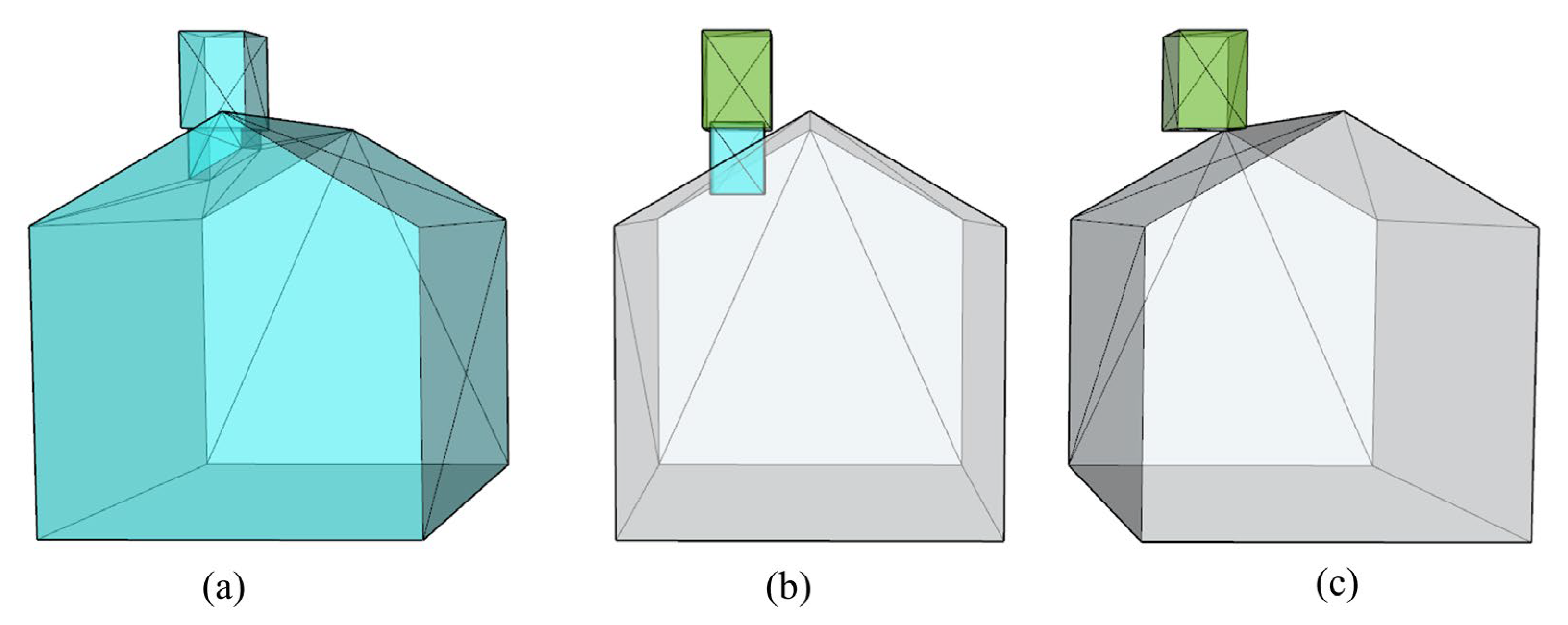
The simplification algorithm of 3D models, which is the key to generate different LODs, has always been a research hotspot in computer graphics [7,8]. Although several classic simplification algorithms have been proposed, most of them are designed for free-form surface models and may not be well applicable to 3D building models. Therefore, scholars have proposed a series of simplification algorithms for 3D building models [9,10,11,12], aiming at their special geometric constraints (vertical, parallel, and coplanar relation). According to the procedural modeling process that has been widely used in architectural design in recent years, most building models are gradually established using components because of their high efficiency [13]. Although these components have strong topological dependence in real space, they are organized as independent meshes in the model modeling process (Figure 1b). There is no connection relationship between the different meshes. When the existing algorithms are directly used to simplify multi-component building models, each component would be simplified independently, leading to the destruction of topological dependence among the components. Consequently, the unreasonable separation of adjacent components (Figure 1c) and possibly inconsistent conclusions of spatial analysis among different LODs may appear. As an important expression means for building models, one of the important features of BIM is componentization. Thus, the above problems are also possible for BIM models. The existing simplification methods mostly focus on the geometric constraint. Although several researchers have begun to consider the texture and semantic relationship of building models, there are few studies that consider the topological relationship between components. Thus, a simplification method for multi-component building models that considers topological dependence needs to be further studied.
To solve the aforementioned problems, a simplification method, which considers the topological dependence among building components as constraints, is proposed. The vertices of building models are first classified into boundary vertices, hole vertices, and other ordinary vertices. For the boundary vertex, the term “angle between the edge and component” (E–C angle), denoting the degree of component separation, is introduced to derive an error metric to produce as much edge collapse occurring inside components as possible. In addition, the quadratic error metric (QEM) algorithm is improved for the hole vertex to address the unexpected error caused by the QEM’s defect. Compared with the traditional method, the proposed method effectively avoids topological inconsistency among different LODs while maintaining the overall appearance features of building models. In addition, the consistency of the visibility analysis among the different LODs is enhanced.
2. Related Work
2.1. Simplification of 3D Building Models
A series of simplification algorithms for 3D models have been proposed—most of them are based on the following classic operations: vertex clustering [14], vertex decimation [15], edge collapse [16], and polygon collapse [17]. The key of these algorithms is to calculate the error metric of geometric primitives (vertices, lines, and faces) in 3D models and remove them sequentially according to the value of the error metric until the target of the simplification rate is reached. The error metric is an index for evaluating the impact of simplification operations on 3D models. Therefore, it is essential to determine the appropriate error metric for the final simplification results of the models. Garland and Heckbert [18] proposed a mesh simplification method based on QEM, which generates a high approximation of the original model by limiting the changes in the local curvature and volume during the simplification process. Due to its excellent performance in geometric feature maintenance, QEM has become a classic algorithm in 3D model simplification. Lindstrom and Turk [19] introduced a new framework that determines which part of the model needs to be simplified by comparing the difference between the rendered images before and after simplification. Inspired by this, Luebke and Hallen [20] developed a perception-driven simplification algorithm. This algorithm evaluates the impact of simplification operations based on psychological models and prioritizes simplification operations that are not easily detectable. Cohen-Steiner and Alliez [21] proposed a simplification method based on variational geometric partition and introduced a new error metric that considers normal deviation to generate a geometric approximation of surfaces. In addition, there are some methods for simplifying 3D models based on the mutual information of viewpoints [22,23]. However, most of the aforementioned methods aim at free-form surface models, which may destroy the geometric structure and local topology when applied to building models.
Considering the unique geometric structure of building models (windows, doors, etc.), many simplification methods have been proposed, which emphasized extracting the geometric structures of building models. Ribelles and Heckbert [9] identified and removed trivial features (protrusions, holes, decorations, etc.) based on the separation plane. Thiemann and Sester [24] improved this method by dividing a building model into several meaningful parts (roof, windows, etc.), and then simplifying the building model by removing the unimportant parts. Rau and Chen [25] defined feature resolution based on the distance between the observer and the building model and generated different LODs by removing unimportant structures at different resolutions. Li and Sun [13] divided the geometric structures of building models into three types: embedded structures, compositional structures, and connecting structures, through convex/concave analysis. Subsequently, they generated different LODs of these structures using a progressive simplification strategy. To automatically generate a simplified building model, Jarząbek-Rychard and Borkowski [26] recognized roof structures based on aerial laser scanning (ALS) data and decomposed them into predefined simple parameter structures. In addition, scholars have begun to pay attention to the semantic relationship of building models to ensure cognitive consistency before and after simplification. Fan and Meng [27] proposed a simplification method for CityGML models subject to semantics. Simultaneously, for the IFC models, Ladenhauf and Berndt [28] proposed a geometric simplification method that considers semantic constraints and expert knowledge. However, the aforementioned methods ignore the topological dependence among the components of building models, which may lead to the separation of neighboring components or distortion of adjacent areas for neighboring components. Thus, a reasonable topology-preserving simplification method for building models needs to be further explored.
2.2. Consistency of Spatial Analysis
As one of the important contents of 3D GIS, 3D spatial analysis has attracted more and more attention. Brasebin and Perret [29] illustrated the impact of 3D data geometric modeling on spatial analysis using the sky view factor. Fisher-Gewirtzman and Shashkov [30] realized visibility analysis by subdividing the urban environment volume into voxels. Ahmed and Sekar [31] showed that 3D volumetric analysis could substantially improve urban space planning and support decision-making processes. Gergelova and Kuzevicova [32] evaluated the suitability of roof surfaces’ potential and suitability for photovoltaic systems based on their geometric parameters. In recent years, BIM models have been increasingly used in spatial analysis. Kota and Haberl [33] conducted daylighting simulation and analysis based on a BIM model and developed corresponding software prototypes. Salimzadeh and Vahdatikhaki [34] developed a parametric modeling platform for the design of a surface-specific photovoltaic module layout on the entire skin of buildings using the surface properties of a BIM model.
In order to improve the accuracy of spatial analysis/simulation, scholars have explored some methods to improve the data quality of building models. Horna and Meneveaux [35] proposed a formal representation of consistency constraints to limit the reconstruction of 3D building models. Ghawana and Zlatanova [36] described the process of topologically correcting 2D features to serve as the basis to create topologically correct 3D city models. Further, Alam and Wagner [37] proposed an automated method to verify and repair the errors of the CityGML model in the aspects of its geometric and semantic consistency. In addition, LODs have been widely used to improve the efficiency of spatial analysis in large-scale city scenes [6]. However, no topological consistency exists among different LODs, which may lead to inconsistent conclusions for 3D spatial analysis (such as view factor analysis and sunshine duration analysis) [6,29]. Therefore, in the simplification process, maintaining topological consistency among different LODs becomes essential. To this end, Biljecki and Ledoux [38] analyzed the impact of different variants (geometric reference) for each LOD on spatial analysis. The research showed that the LOD1 model with a specific geometric reference might be more accurate than the LOD2 model in spatial analysis. Thus, it is better to develop a corresponding simplification strategy for each spatial analysis application. Following this principle, a specific simplification method for visibility analysis is proposed.
3. Methodology
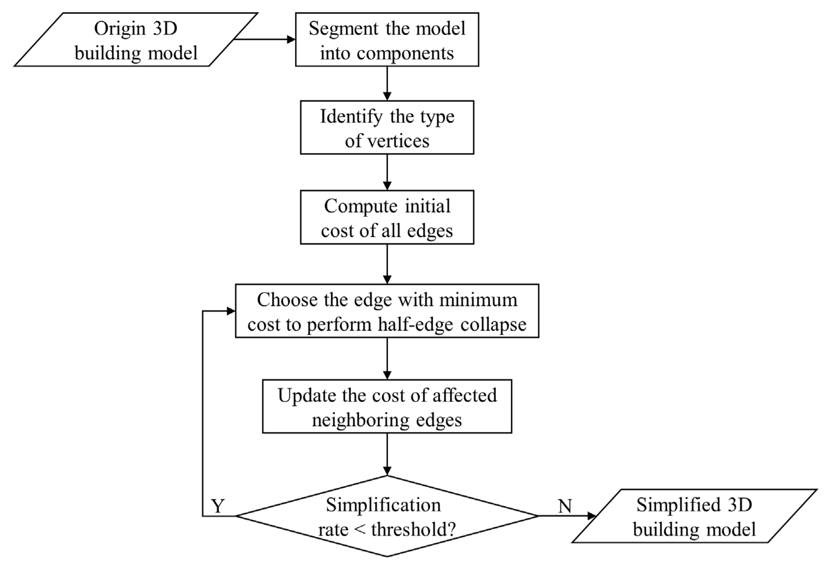
In this research, we chose half-edge collapse as the basic simplification operation for the following reasons: (1) we do not need to calculate the coordinates of the new vertex after each collapse, thereby improving the efficiency of the proposed method; (2) for the multi-component building model, a new vertex may destroy the topological dependence. In this case, the optimal vertex coordinates are challenging to determine. The building models used in this paper are all in the form of triangular meshes by default; models of other forms (BIM, 3D point clouds, etc.) should be converted into triangular meshes prior to the simplification process. The flow of the proposed method is illustrated in Figure 2. First, we segmented the building model into different components based on whether the meshes were completely connected. Next, we classified vertices into three types: boundary, hole, and other ordinary vertices. Finally, for different vertex types, we defined different error metrics, with which the edge cost is calculated to maintain the topological dependence among building components. Edge collapse has local relevance, and its cost is affected by the adjacent triangles. Therefore, the cost of adjacent edges must be updated after each collapse. The method terminates when the simplification rate, which is defined as the number of removed triangles divided by the number of triangles in the original model, reaches a user-specified threshold.
3.1. Component Segmentation of Building Models
In recent years, most building models are established gradually using components. Nevertheless, multiple components with the same shape may be merged into an aggregate structure, which can used as the basic unit of data organization. In this condition, the model cannot meet the requirements of the proposed algorithm. Thus, we need to segment the building model into different components based on whether the meshes are actually successive.
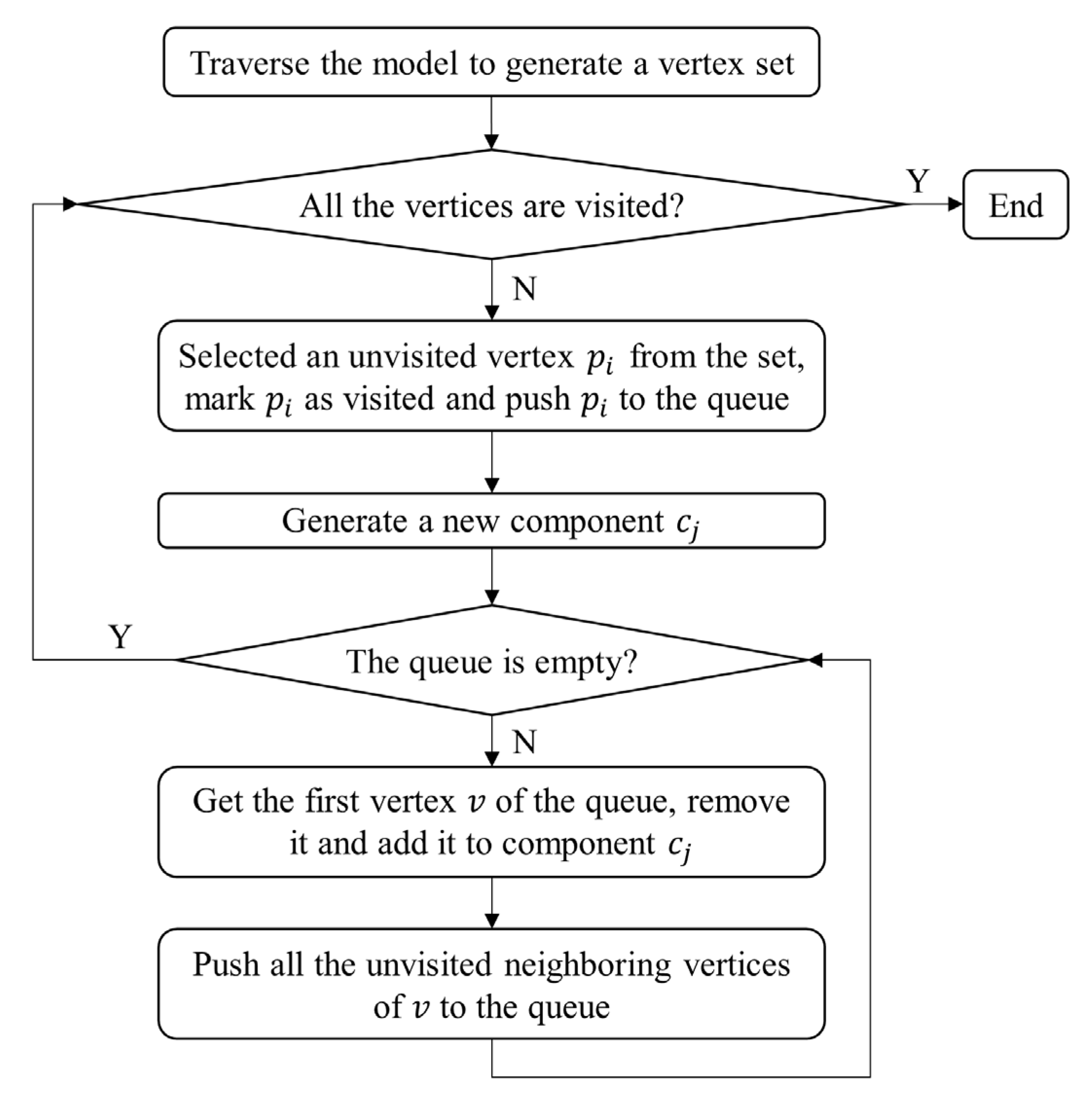
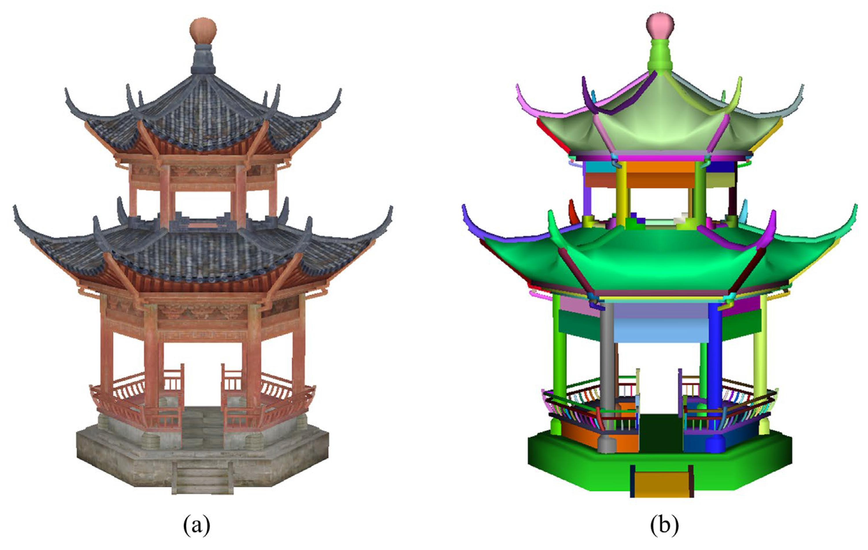
Specifically, the segmentation of building models is based on the breadth-first search (BFS) algorithm. This segmentation can be regarded as classifying disconnected subgraphs in the graph, which is an application of the BFS algorithm. Each subgraph is an independent component. In addition, the segmentation is fully automated. The flow is detailed in Figure 3. First, we traversed all meshes of the building model, generated a vertex set P, and marked all vertices as unvisited. Then, we chose a random unvisited vertex from the set as the starting vertex. All the vertices that are directly or indirectly connected (two vertices are defined as indirectly connected when they are connected by other vertices) to it were classified into the same component and marked as visited. In the segmentation process, we created a queue as a container for vertices, and unvisited vertices belonging to the same component were continuously pushed into the queue. When the queue is empty, it indicates that all the vertices of this component are extracted. This process was repeated. When all the vertices were visited, the algorithm terminated. These results are shown in Figure 4, and the different components are marked with different colors.
3.2. Classification of Vertices
The topological dependence considered in the proposed method is defined as the topological relationship between components. Three-dimensional building models are generally organized by geometric primitives (such as vertices, edges, and triangles). Their topological relationship is mainly expressed as the spatial relationship among these geometric primitives. There are several types of topological relationships, which are connectivity, adjacency, and inclusion [39]. Nowadays, the popular componentized modeling generally divides the building model into multiple parts, and each part will be modeled independently to form different components. Similar to the above geometric primitives, these components are connected in real space and also have strong topological dependence (connectivity, adjacency, and inclusion) with each other. However, they are organized as independent meshes in the data structure. Each component is simplified independently, which may ignore its influence on other neighboring components, leading to unreasonable damage. In our study, the topological relationship of components is expressed and constrained through vertices. To maintain the topological relationship of components, the first is to classify the type of vertices.
3.2.1. Types of Vertices
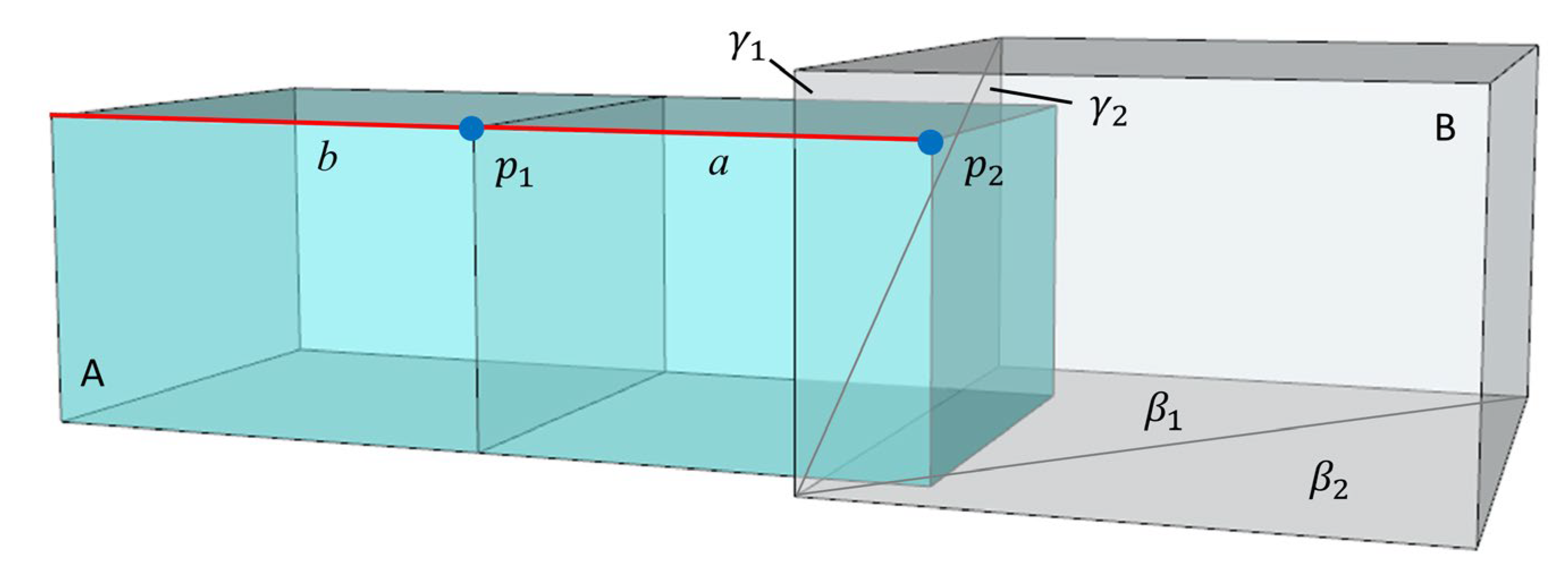
As shown in Figure 5, edge a intersects with component B, and its collapse can easily cause the separation of components. It is defined as the boundary edge. There is no intersection between edge b and component B, and thus it is defined as an ordinary edge. Edge c is inside component B, and its two vertices are both inside component B. The vertex after the collapse is still in component B, which does not cause the separation of components, meaning it is also defined as the ordinary edge. The vertex, which is located inside the intersection component, in the boundary edge is defined as the boundary vertex, whereas the other is the ordinary vertex. As shown in Figure 5, for boundary edge a, vertex p1 is outside component B, which is defined as the ordinary vertex, and the other vertex p2 is inside component B, which is the boundary vertex. Both vertices of the ordinary edge are defined as ordinary vertices. The collapse of edge a can be divided into two cases: and . Although both operations are aimed at the same edge, their influences are completely different. To avoid confusion, we defined the collapse of the boundary vertex to an ordinary vertex as the collapse of the boundary vertex. The extraction of boundary vertices is complex, as elaborated in the followed section.
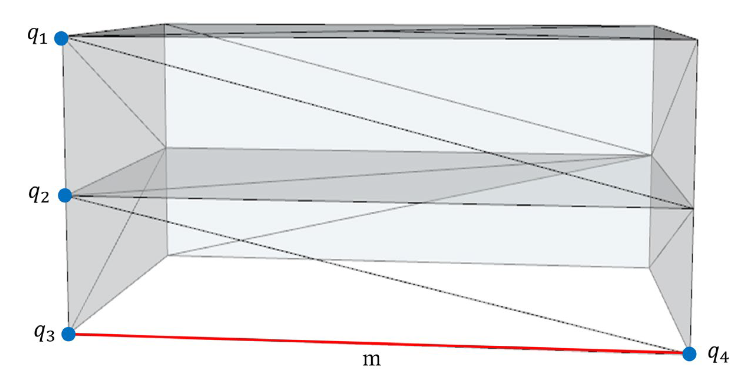
In the building components, the edge with only one adjacent triangle is defined as the hole edge, and its two vertices are recorded as hole vertices. The calculation rules of the QEM allow such edges to be simplified earlier than the actual demands. Therefore, a new error metric should be introduced. The error metric of the QEM algorithm is defined as the sum of the squares of the distance from the new vertex to the adjacent surface of the original vertex. As shown in Figure 6, m is the hole edge, and q3 and q4 are the hole vertices. In terms of visual effects, the collapse of q3 to q2 causes a greater error than that of q2 to q1. However, owing to the lack of two adjacent faces at the bottom of q3, the error metric of computed by the QEM algorithm is zero, and the collapse is always preferentially executed.
3.2.2. Extraction Rules of Boundary Vertices
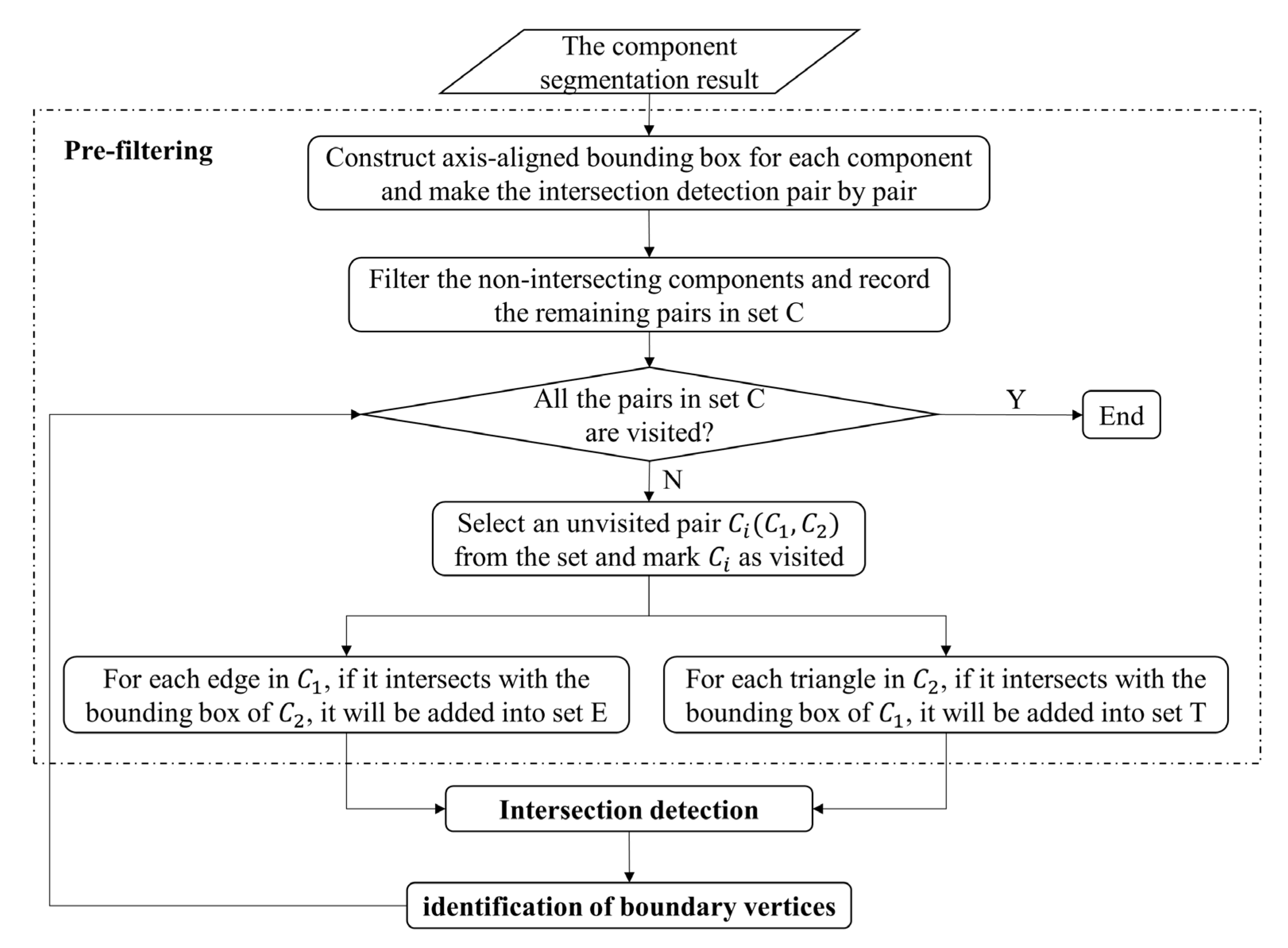
For multi-component building models, topological dependence is mainly represented as intersecting or attaching (components bind tightly on certain planes) among components—components have overlapping parts. The maintenance of topological dependence for building components primarily emphasizes the maintenance of overlapping parts among components. In this case, we can extract the boundary vertices through the intersection of edges and triangles. Then, the simplification of overlapping parts among components will be constrained based on these boundary vertices. Thus, the core lies in how to extract the boundary vertices of components correctly. In addition, the axis-aligned bounding boxes (AABB) of the components are constructed for pre-filtering to speed up the efficiency of intersection detection. The flow is illustrated in Figure 7.
(1) Pre-filtering
Step 1: Construct AABB of the building components and allow the intersection detection to, pair by pair, filter the non-intersecting components. The remaining pairs are recorded and marked as unvisited in set C.
Step 2: Select an unvisited pair from the set and mark Ci as visited. For each edge in C1, when it intersects with the bounding box of C2, it is added to set E. As shown in Figure 8, edge b does not intersect with the bounding box of component B. It will be filtered and will not be added to set E.
Step 3: For each triangle in C2, when it intersects with the bounding box of C1, it is added to set T. As shown in Figure 8, triangles and do not intersect with the bounding box of component A. They are filtered and will not be added to set T. In component B, only the triangles and intersect with the bounding box of component A and participate in the next intersection detection, significantly improving the calculation efficiency.
(2) Intersection detection
For each edge in E, such as edge a in Figure 8, when it intersects with any triangle in T, such as triangles and in Figure 8, it is the boundary edge. The general idea of judging whether an edge intersects with a triangle is as follows: when the edge is parallel to the plane where the triangle is located, there is no intersection. Otherwise, we compute the coordinates of the intersection vertex and determine whether the vertex is within the triangle.
(3) Identification of boundary vertices
For each boundary edge, the boundary vertex is determined according to the angle between the edge and the normal vector of the intersection triangle. Specifically: taking Figure 8 as an example, we connect both vertices of edge a to form a vector and calculate the angle between it and the normal vector of triangle . If the angle is acute, the back vertex (p1) of the vector is the boundary vertex, whereas the front vertex (p2) of the vector is the boundary vertex. In addition, when the edge passes through the component, both vertices are outside the component. The collapse of any vertex will cause the separation of components. Thus, both vertices are regarded as boundary vertices.
3.2.3. Supplementary Rules
For some special building components, the general aforementioned extraction rules cannot guarantee the accuracy of the extraction result. Therefore, we propose the following special extraction rules:
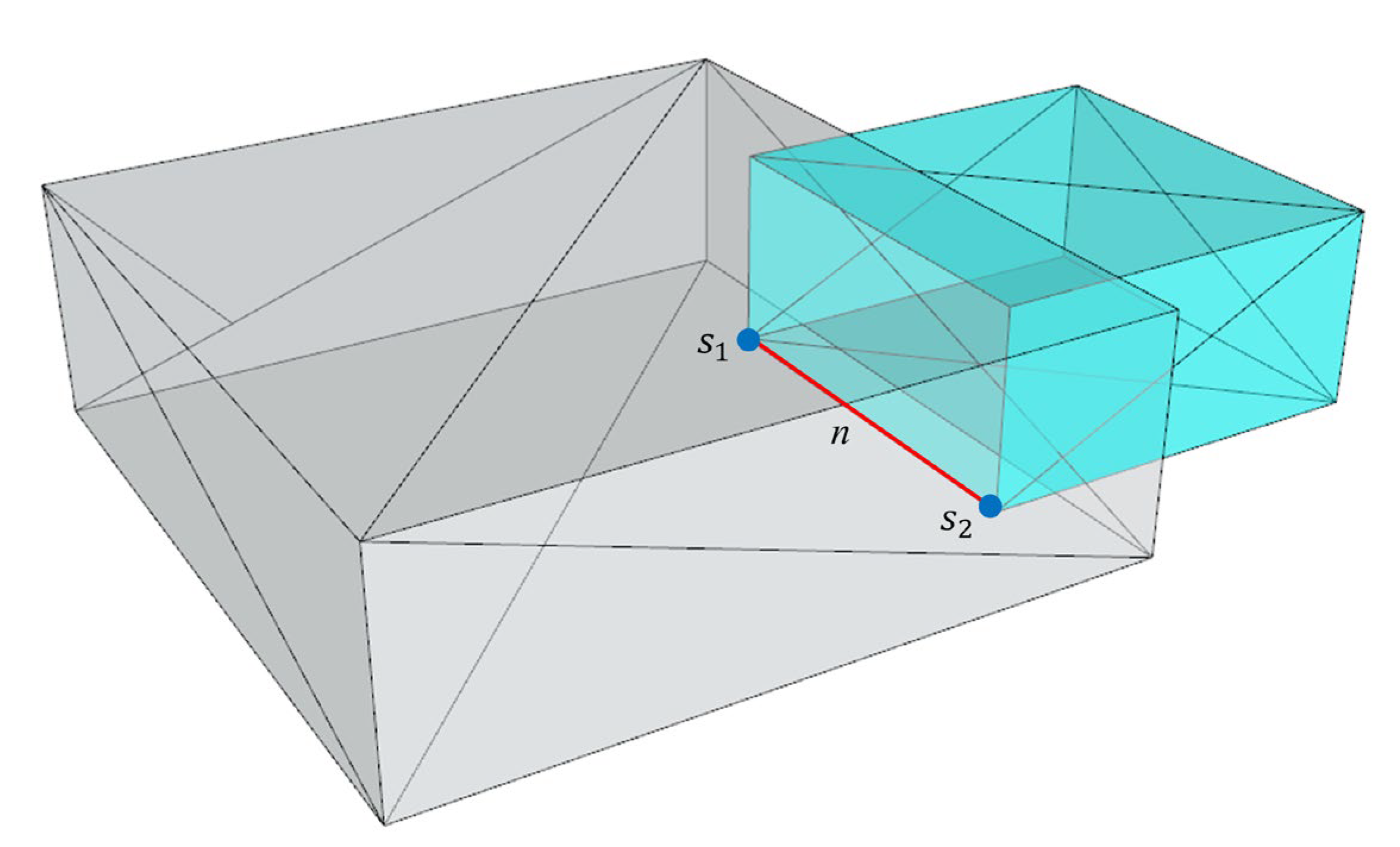
- When a vertex has the characteristics of a boundary vertex and a hole vertex simultaneously, it will be recorded as a boundary vertex. Although the number of adjacent triangles of the edges where these vertices are located is also one (Figure 9), it is caused by modeling errors. These vertices cannot represent the holes of the building models. To prevent these boundary vertices from being simplified first, the holes formed by them will be triangulated to meet the requirements of the proposed method. The retriangulation algorithm used in our method was proposed by Weatherill and Hassan [40]. As shown in Figure 9, edge n has only one adjacent triangle, and the vertical plane where it is located is not closed. However, its vertices s1 and s2 have been recognized as boundary vertices to restrain. Therefore, they are not defined as hole vertices.
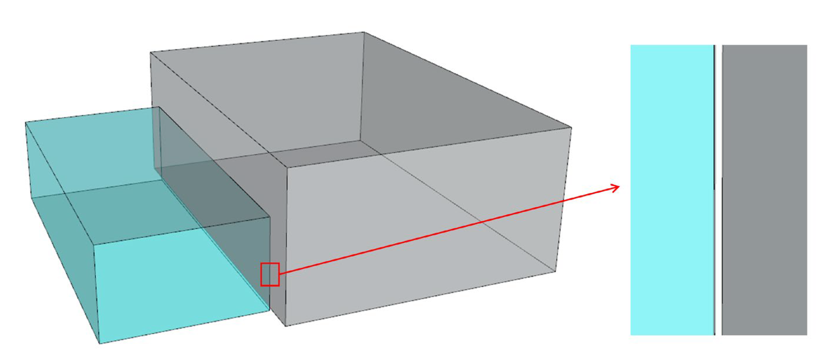
- For multi-component building models, topological dependence is mainly represented by intersecting or attaching among components. However, there are also some special conditions, such as visual attaching. As shown in Figure 10, both components are visually attached. However, there is a small gap between them. In this case, the method based on intersection detection cannot correctly extract the boundary vertices, and the separation of components may still occur during the simplification process. To address this challenge, we temporarily extended the bounding box and the edge to a certain extent during the intersection detection based on the buffering idea, with an amplitude of 1% of the length.
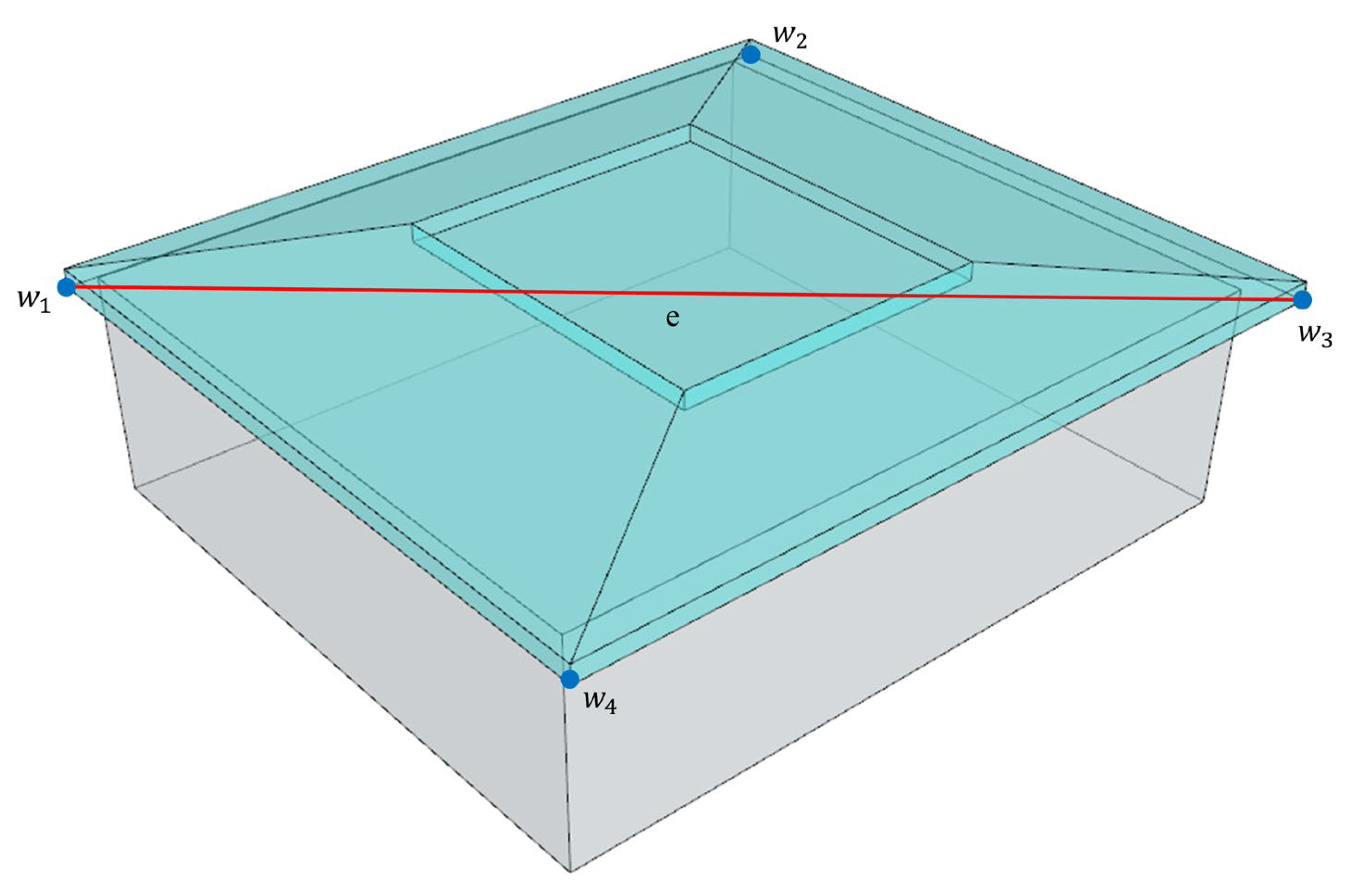
- The supplementary rule (when an edge passes through a component, such as e in Figure 11, both vertices of the edge are regarded as boundary vertices) defined in Section 3.2.2 solves the problem of interleaved components. However, when facing intersection components with an “embedded” relationship, the extraction result may be incomplete. For instance, as shown in Figure 11, the bottom quadrilateral of the roof is composed of two triangles, and its area is larger than the area of the wall, forming an “embedded” relationship. During intersection detection, the hypotenuse e intersects with the wall and passes through it. Both vertices of the edge can be identified as boundary vertices . According to the rule of intersection detection, no edge intersects with the wall for the other two vertices of the bottom quadrilateral—they are recognized as ordinary vertices. However, they also easily collapse during the simplification process, causing separation between the roof and the wall. To solve this kind of problem, we propose a supplementary rule: when an edge passes through a component and the normal vectors of its two adjacent triangles are parallel, the other two vertices of both triangles are also regarded as boundary vertices. The final extraction results are shown in Figure 12.
3.3. Simplification Based on Cost of Edges
3.3.1. The E–C Angle
The large number of building components leads to a large number of boundary vertices, which may even exceed half of the total number of vertices in the model. If all boundary vertices are prohibited from collapsing, the simplification rate of the building model will be severely restricted. Thus, it is vital to achieve a balance between the simplification rate and the simplification quality.
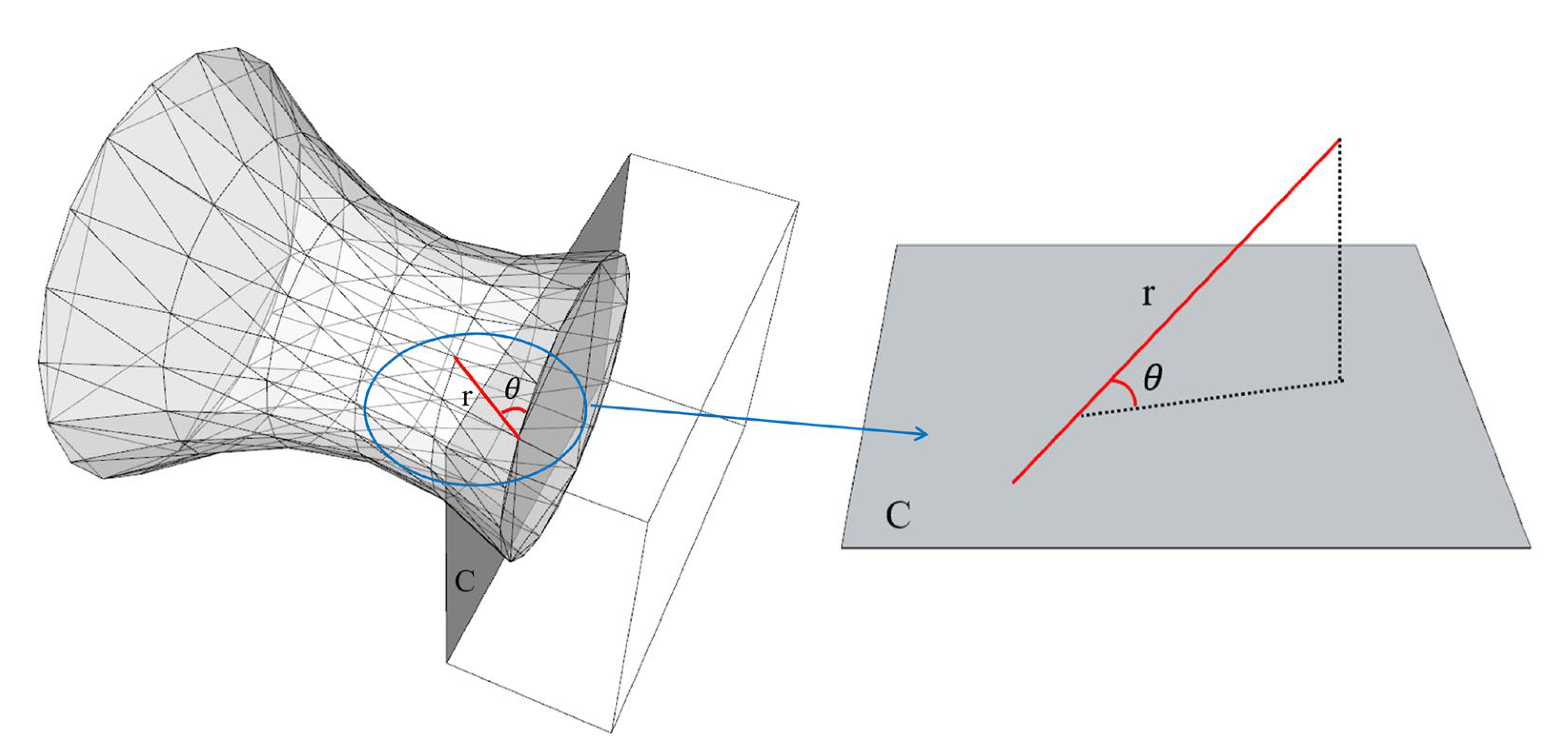
The angle between the edge and component, named the “E–C angle”, is an essential indicator that determines the priority of edge collapse and also an important factor affecting the degree of component separation. There is no definition of the angle between the 2D edge and 3D component. Therefore, we introduce the definition of the collapse reference plane to replace the component to calculate the angle. In this study, the collapse reference plane is defined as the triangle intersecting the edge, such as plane C in Figure 13. When the angle is 0°, the vertex remains inside the component after the collapse, and the collapse does not cause the separation of components. As the angle increases, the crack between the components caused by the edge collapse becomes clearer. In addition, when the edge is perpendicular to the component, the destruction caused by its collapse reaches a maximum. Therefore, emphasis should be placed on limiting the edges with larger angles, whereas almost parallel edges should be less restricted or even not restricted.
The parameter in Figure 13 represents the E–C angle. When approaches 0° (), the cost of the edge mainly depends on the component deformation caused by the edge collapse. When approaches 90° (), the cost of the edge mainly depends on the angle. At this time, the cost is extremely high, resulting in the edge not being simplified.
3.3.2. Error metric for Simplification
The simplification of building models is achieved by reducing the number of edges, which is called edge collapse. For each collapse, the edge with the least impact on the model was selected based on the error metric. Once the error metric is determined, the simplification is performed in the order of edge costs until the corresponding simplification rate is reached. The classic method to calculate the error metric is the QEM algorithm, which uses a quadratic error as the error metric. In particular, for each triangle t of the original mesh, this method defines a quadric , whose value is the squared distance from a vertex to the plane containing the triangle t. The quadric of vertex v is the sum of the quadrics on its neighboring triangles weighted by the triangle area:
Additionally, the cost of is defined as .
The QEM algorithm can maintain the geometric characteristics of building models. However, it does not consider the topological dependence among components and cannot avoid component separation for building models. To solve this problem, boundary vertices should be considered when calculating the cost of the edge. We use the E–C angle to define a new error metric, which is as follows:
The aforementioned is computed as . The parameter a represents the basic cost ratio of the collapse—when the E–C angle is 0°, the extra cost must be paid for the collapse of the boundary vertex compared with the ordinary vertex. This ensures that the collapse is performed inside the components more, thereby better maintaining the topological dependence of building models. For each model, the optimal value of parameter a is summarized by multiple experiments combined with manual judgment. We will analyze the value of a and its influence on the simplification results of building models in Section 4.2 in detail. In addition, when two boundary vertices are located inside the same component, the E–C angle is challenging to compute. At this time, it was defined as 0°. The cost of the edge depends not only on the QEM but also on the basic cost ratio a. represents the improved QEM error metric. The error metric of the hole vertices calculated by the traditional QEM algorithm was zero, which is inconsistent with reality. We used the length of the collapsed edge to replace the distance between the vertex after the collapse and the adjacent triangles of the collapsed vertex to calculate the error metric. Taking q3 in Figure 6 as an example, q3 is the hole vertex and . We used the length of q3q2 to replace the distance between q2 and the adjacent triangles of q3. The length of q3q2 represents the maximum possible value of the distance between q2 and the adjacent triangles of q3, which increases the error metric to a certain extent and can better maintain the characteristics of building models.
4. Results and Discussion
To verify the capabilities of the proposed method, simplification experiments were performed on three building models: a traditional Chinese building model with complex structures (pavilion), a modern building model with simple structures (apartment), and a modern building model with complex structures (house). We begin by providing the simplification results for the three models and compare them with the results of the QEM and vertex clustering methods to demonstrate the advantages of the proposed method in terms of overall appearance preservation. Then, the influence of parameter a on the simplification results is analyzed and evaluated. Finally, the consistency of the visibility analysis among the different LODs is verified.
4.1. Simplification Effect
In this section, we compare the simplification effects of different methods under the same simplification rate. The simplification statistics for the three building models are presented in Table 1, and the specific simplification results are shown in Figure 14. Based on the results of many experiments, parameter a of the three models was determined to be 2.0, 1.5, and 5.0, respectively. We will discuss how to take the value of parameter a and its influence on the model simplification effect in detail in Section 4.2.
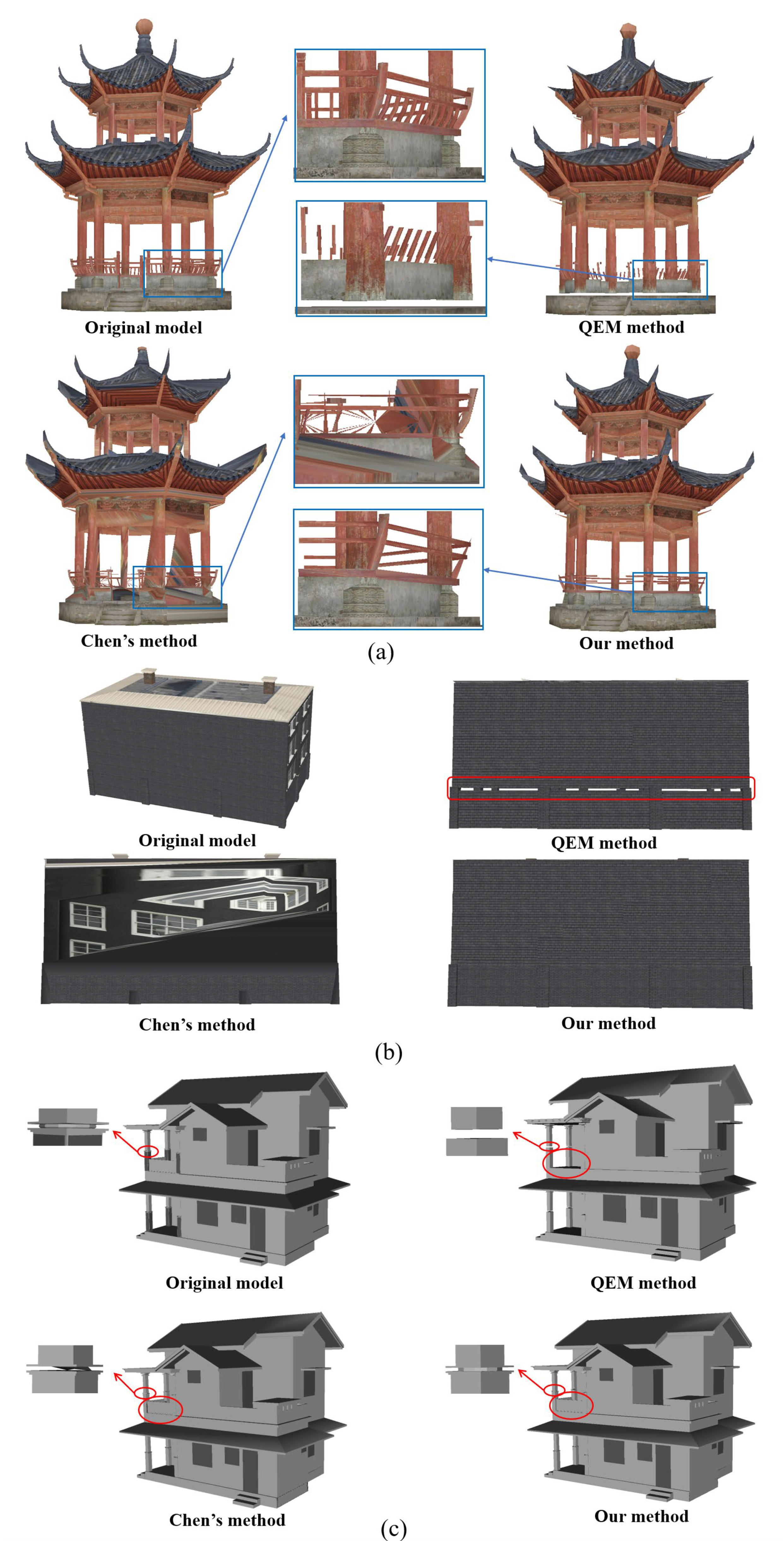
To demonstrate the effect of the proposed method on preserving the overall appearance features, we compared the proposed method with the QEM method [18] and an improved texture-related vertex clustering method proposed by Chen [41]. The main reasons for the formation of cracks are the collapse of tiny components and the collapse of tiny structures at the intersection of the components. As shown in Figure 14a, the deformation of the railing component caused by the QEM method corresponds to the collapse of tiny components. Although no cracks were formed, the collapse caused apparent damage to the overall appearance of the pavilion. The irregularity of the modeling process caused some components in the railing to form features similar to the hole vertex. In the QEM algorithm, these vertices have an error metric of zero and are always simplified first. To retain the characteristics of these components, a high cost is set uniformly so that the components that should be simplified earlier in Figure 14a are retained, which does not match reality. For the vertex clustering method, multiple topologically non-adjacent components in the railing are clustered together, causing huge damage to the appearance. For the proposed method, the holes formed by these vertices are retriangulated in Section 3.2.3, and the simplification result is better. Simultaneously, the separation of the base with the body for the pavilion belongs to the collapse of tiny structures at the intersection of components, forming an apparent crack. The proposed method preserves the microstructure of the base by restricting the collapse of boundary vertices, avoiding separation, and achieving a better visual effect. In contrast, although the vertex clustering method also maintains the topological relationship of the building model, it causes obvious texture distortions, resulting in poor visual effects. As shown in Figure 14b, the structure for the apartment is simple, which means the number of boundary vertices is small. Thus, a higher simplification rate can be reached. As the simplification rate increases, the tiny structures inside the components collapse, causing cracks to appear. Similar to the pavilion, although the vertex clustering method did not cause the separation of components, it causes greater texture distortion. As shown in Figure 14c, the internal connection component of the pillars for the house is removed, leading to the destruction of topological dependence. Although the component is small, it connects the different parts of the pillar. Its collapse destroys the integrity of the pillar, and its visual impact is much higher than its error metric. Additionally, fences among the pillars are removed. For the proposed method, the visual effect of the other components changes little while avoiding the collapse of connection components in the pillar and the fence. For the vertex clustering algorithm, because of the lack of texture in the house, the simplification result is good. In addition, owing to the small volume of the connecting components, the simplification rate of the house is limited to some extent while maintaining its integrity.
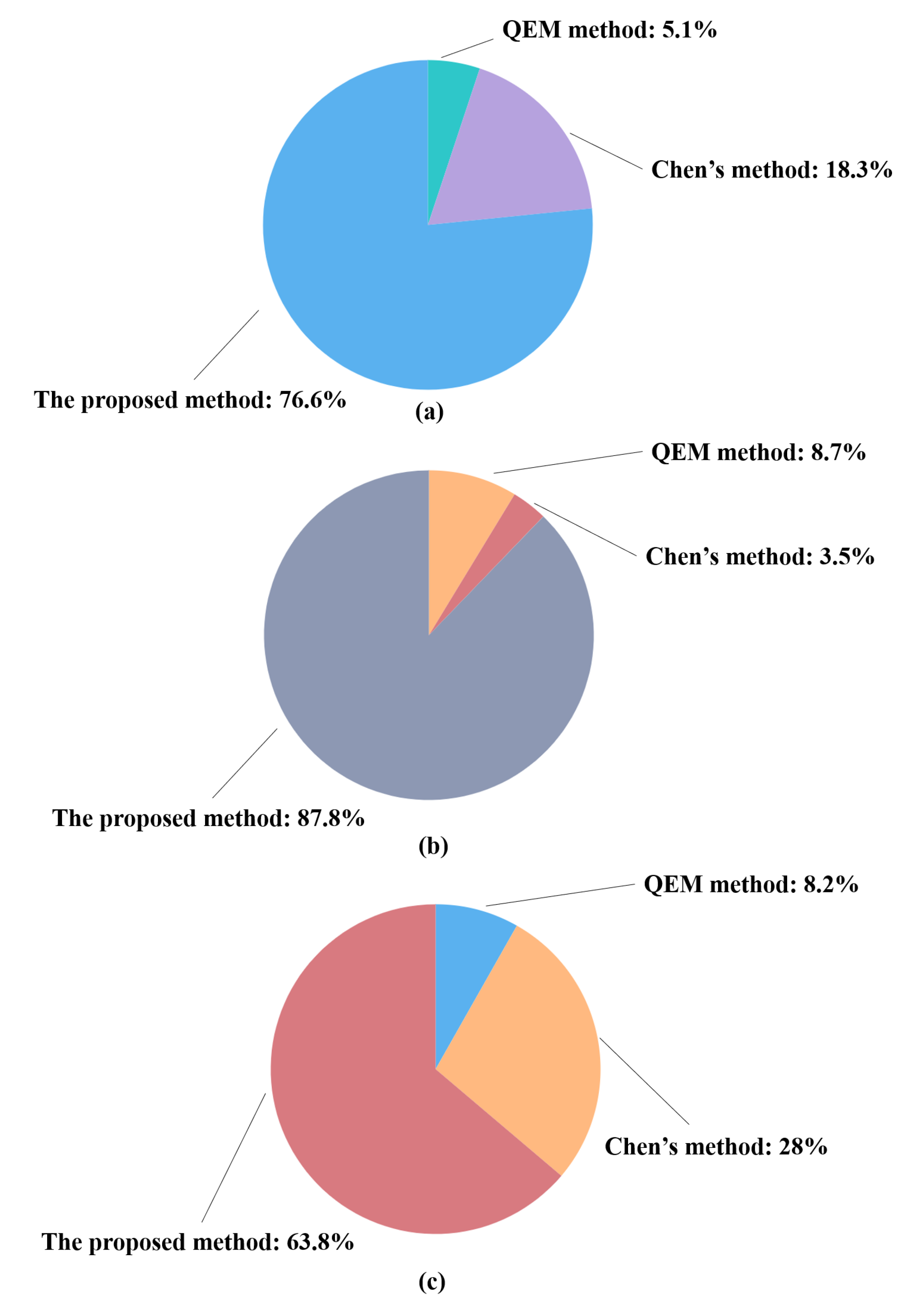
In order to analyze the simplification effect of the proposed method quantitatively, we organized a small-scale user study in the form of an online questionnaire. There are 235 participants in this user study, including 137 people engaged in cartography or GIS-related work (professionals) and 98 people engaged in other work (nonprofessionals). The participants’ age mainly ranges from 18 to 50. For the three models, we show the simplification results derived from different simplification methods. The users can choose the best in their perspective. After sorting out the users’ questionnaire feedback, the results of the user study are as follows (Figure 15): For the pavilion and apartment models, 76.6% and 87.8% of users thought that the proposed method offers a better experience, respectively. For the house model, due to its lack of texture, the difference between Chen’s method and our method is not obvious. A total of 63.8% of users thought the simplification effect of our method is better. In summary, we can draw the following conclusions: most users think that the simplification effect of the proposed method is better than that of the traditional method.
4.2. Analysis of Parameter Influence
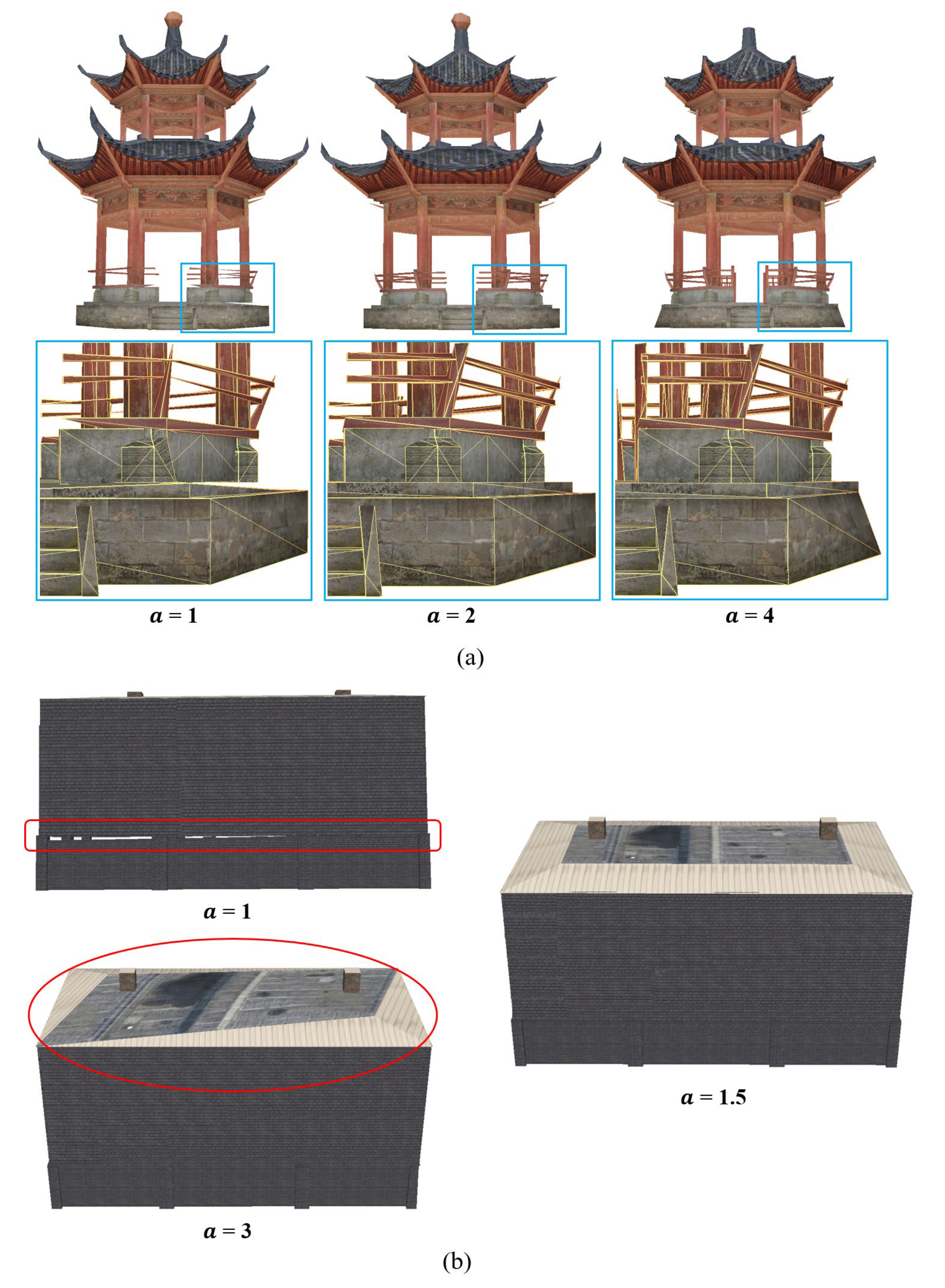
To further analyze the influence of the parameters on the simplification result, a series of experiments was performed on different models independently. The related information for these models is shown in Table 2. According to Section 3.3.2, the factors that affect the error metric include the basic cost ratio a and angle . was automatically calculated. In contrast, the value of a is summarized by multiple experiments combined with manual judgment. Our experiments suggest that a is generally set in the range [1,3] for simple models and the range [2,8] for complex models. We take two typical models, the pavilion (Figure 16a) and the apartment (Figure 16b), as examples to analyze the influence of parameter a in detail. For the pavilion, when the value of parameter a is 1 (too low), the costs of boundary vertices are small, which may be smaller than those of ordinary vertices inside components. The edge collapse would tend to occur at the boundary of components, and the problem of component separation would follow. In this case, although its visual effect is improved compared with the QEM algorithm, the problem caused by the collapse of tiny structures is still not completely solved. As the value of a increases to 2, the collapse operation tends to occur inside the components, and the connection relationship among components is better preserved. The problem of component separation is solved. As a continues to increase, the collapse operation is further concentrated inside the components, which may lead to oversimplification of the pavilion. For example, when a is 4, the costs of the cornice (ordinary vertices) are smaller than those of the railing (boundary vertices). In this case, although the characteristics of the railing are better preserved, the eave is oversimplified, and the top component of the pavilion is completely removed. For the apartment, the experimental results show that the values of a have a similar influence on the simplification effect of different building models.
4.3. Consistency of Visibility Analysis among Different LODs
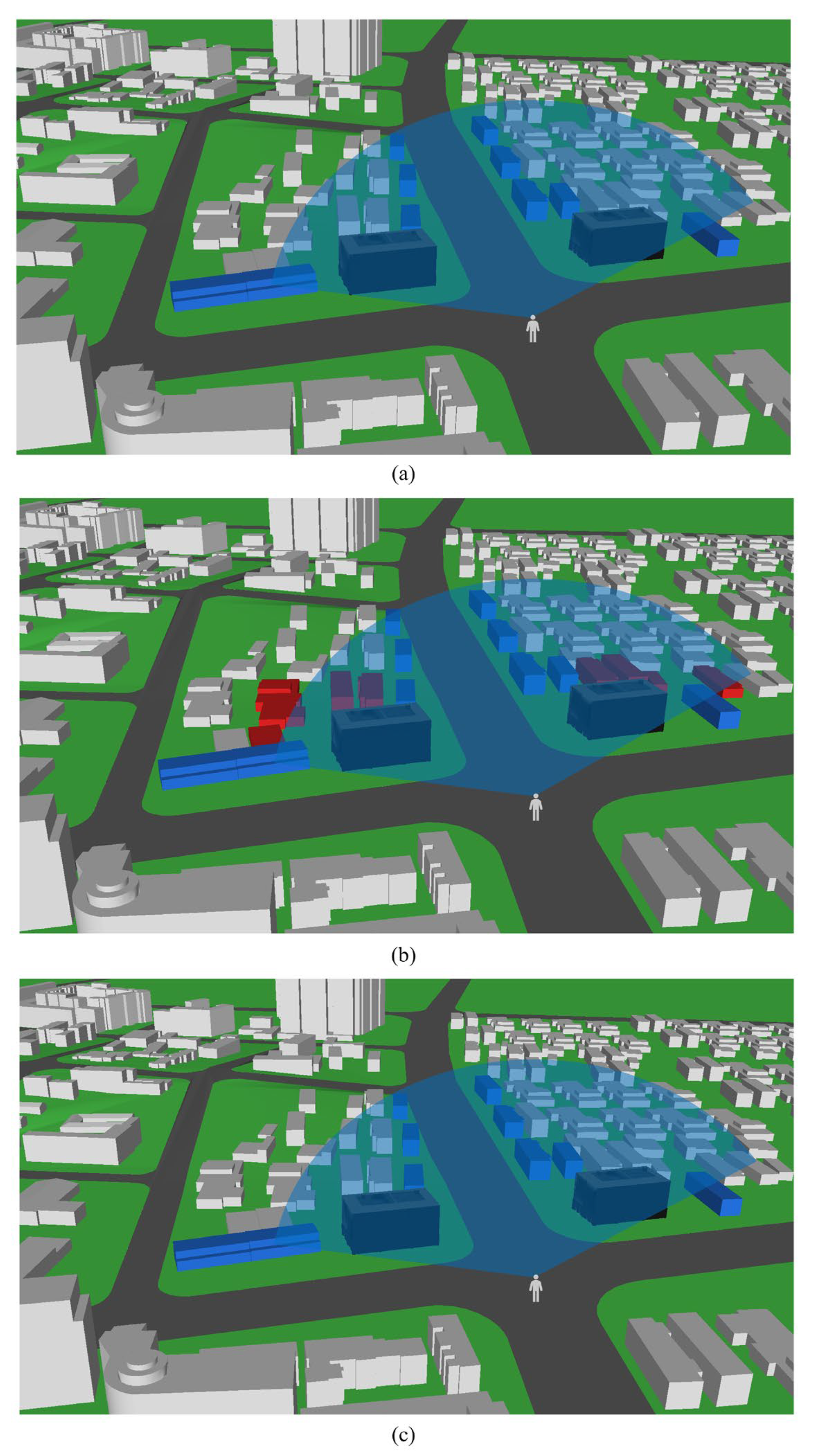
We performed a set of comparative experiments based on OpenSceneGraph (OSG) to determine the effectiveness of the proposed method in maintaining the consistency of visibility analysis among different LODs. The results are presented in Figure 17. The textured building models that block the view in the three scenes are the original model, the simplified model of the QEM method, and the simplified model of the proposed method (for the apartment model with an 80% simplification rate, the specific simplification effect can be seen in Section 4.1). Other buildings are used to show the conclusion of visibility analysis (the number of visible buildings under the current viewpoint). The details of these buildings have no influence on the conclusion of visibility analysis; therefore, some simple models are used instead. The viewpoints, view angles, and view distances were all the same in the three scenes. The visible buildings using the original model for visibility analysis are marked in blue, and the number of visible building models is nine. The difference in results between the model generated by the other methods and the original model is marked in red. The number of visible building models for the QEM method is 17, which is significantly different from that of the original model. In contrast, the simplified model of the proposed method yields the same results as the original model. In addition, the number of visible buildings was also nine, proving its effectiveness.
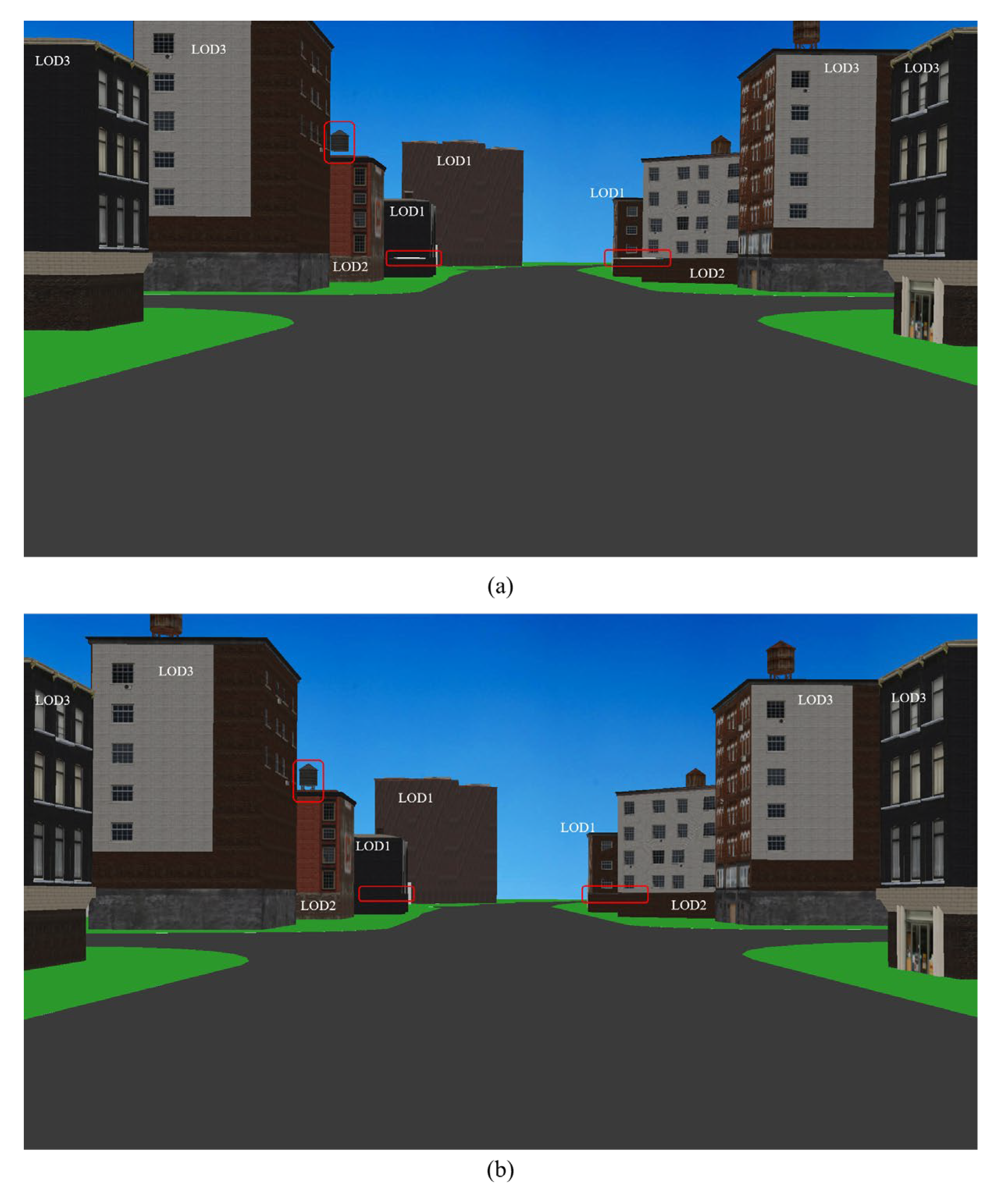
As a supplement, we find an area with LOD1~LOD3 models to prove the performance of our method. The visualization of 3D city scenes is shown in Figure 18. The view is at the street level, which is commonly used when browsing 3D city scenes. From far to near, the buildings in the scene are, respectively, LOD1~LOD3 models under different simplification rates. The CityGML standard has high requirements for the quality of building models. For example, the information such as model topology and semantics needs to be included. In addition, the simplification methods designed for the CityGML standard usually focus on the preservation of specific features and cannot set the simplification rate freely. In order to compare the simplification effect at various simplification rates, we did not use the LODs defined by the CityGML standard but defined the LODs using the simplification rate of models. We replaced the LOD3 models with models with a 0–30% simplification rate, the LOD2 models with models with a 30–70% simplification rate, and the LOD1 models with models with a 70–95% simplification rate. Figure 18a and Figure 18b represent the visualization effects of the QEM method and the proposed method, respectively. For the LOD3 models, the simplification effects of the two methods are basically the same. For the LOD2 models, the problem of component separation occurs for the models simplified by the QEM method. For example, the bottom of the water tower on the roof of the left building is completely simplified, causing the water tower to hang in the air. A semi-separation occurs in the middle of the right building, but it is not obvious in the city scene. For the LOD3 models, the problem of component separation in the QEM method is obvious, and the two distant buildings both have an obvious separation. In contrast, the proposed method avoids this problem, and the visualization effect is better.
In the small-scale user study in Section 4.1, we also conducted a questionnaire survey on the visual effects of the two scenes. The results show that 79.8% people thought that the visualization effect of our method is better.
5. Conclusions
For multi-component building models, a novel simplification method was proposed to preserve the overall appearance features of building models while maintaining the topological dependence of components in the simplification process. In this method, the vertices of building models are classified into boundary vertices, hole vertices, and other ordinary vertices. Subsequently, the unreasonable separation of components is effectively avoided based on the constraints of collapse for the boundary vertex. Simultaneously, an improvement to the QEM algorithm was developed for hole vertices to solve the unexpected error caused by the QEM defect. The results of the user study in Section 4.1 demonstrate that most users think that the simplification effect of the proposed method is better than that of the traditional methods. In addition, the results of comparative experiments in Section 4.3 show that the conclusion of visibility analysis for the proposed method is more accurate. The proposed method emphasized the maintenance of topological consistency. However, it does not make full use of the semantic information of building models. Thus, topological synthesis for components with the same semantics could be an important goal for future research. Parameter a in this study was still manually assigned. Although the simplification results are good, it is hard to meet the efficiency requirements of large-scale city scenes. Therefore, the automated determination of parameter a for building models will be considered in our future research. In addition, the maintenance of consistency for spatial analysis is a significant challenge, and this study only focused on its small fraction. Hence, achieving better consistency for other kinds of spatial analysis among different LODs is a direction worthy of long-term exploration.
Author Contributions
Conceptualization, Biao Wang; methodology, Biao Wang, Guoping Wu, and Jiangfeng She; software, Biao Wang and Qiang Zhao; visualization, Yaozhu Li and Yiyuan Gao; writing—original draft, Biao Wang; writing—review and editing, Jiangfeng She and Guoping Wu. All authors have read and agreed to the published version of the manuscript.
Funding
This research was funded by National Natural Science Foundation of China, grant number 41871293 and grant number 41371365.
Data Availability Statement
The data presented in this paper are openly available at http://0-doi-org.brum.beds.ac.uk/10.5281/zenodo.4994286 (accessed on 20 June 2021).
Acknowledgments
Thanks to the website https://www.cgtrader.com/ (accessed on 18 June 2021) for providing the free building models.
Conflicts of Interest
The authors declare no conflict of interest.
References
- Xie, J.; Feng, C.-C. An Integrated Simplification Approach for 3D Buildings with Sloped and Flat Roofs. ISPRS Int. J. Geo-Inf. 2016, 5, 128. [Google Scholar] [CrossRef] [Green Version]
- Clark, J.H. Hierarchical geometric models for visible surface algorithms. Commun. ACM 1976, 19, 547–554. [Google Scholar] [CrossRef]
- Gröger, G.; Kolbe, T.H.; Nagel, C.; Häfele, K.-H. OGC city geography markup language (CityGML) encoding standard. Open Geospat. Consort. 2012. [Google Scholar]
- Fai, S.; Rafeiro, J. Establishing an appropriate level of detail (LoD) for a building information model (BIM)-West Block, Parliament Hill, Ottawa, Canada. ISPRS Ann. Photogramm. Remote Sens. Spat. Inf. Sci. 2014, 2, 123. [Google Scholar] [CrossRef] [Green Version]
- Uusitalo, P.; Seppänen, O.; Lappalainen, E.; Peltokorpi, A.; Olivieri, H. Applying level of detail in a BIM-based project: An overall process for lean design management. Buildings 2019, 9, 109. [Google Scholar] [CrossRef] [Green Version]
- Besuievsky, G.; Barroso, S.; Beckers, B.; Patow, G. A Configurable LoD for Procedural Urban Models intended for Daylight Simulation. In Proceedings of UDMV; Eurographics Association: Geneva, Switzerland, 2014; pp. 19–24. [Google Scholar]
- Rossignac, J. 54 Surface Simplification and 3d Geome-Try Compression. Triangle 2004, 2, 4. [Google Scholar]
- Wang, Y.; Zheng, J.; Wang, H. Fast mesh simplification method for three-dimensional geometric models with feature-preserving efficiency. Sci. Program. 2019. [Google Scholar] [CrossRef]
- Ribelles, J.; Heckbert, P.S.; Garland, M.; Stahovich, T.; Srivastava, V. Finding and removing features from polyhedra. In Proceedings of DETC; American Society Of Mechanical Engineers: New York, NY, USA, 2001; pp. 1–10. [Google Scholar]
- Kada, M. Scale-dependent simplification of 3D building models based on cell decomposition and primitive instancing. In Proceedings of the International Conference on Spatial Information Theory, Melbourne, Australia, 19–23 September 2007; Springer: Berlin/Heidelberg, Germany; pp. 222–237. [Google Scholar] [CrossRef]
- Zhao, J.; Zhu, Q.; Du, Z.; Feng, T.; Zhang, Y. Mathematical morphology-based generalization of complex 3D building models incorporating semantic relationships. ISPRS J. Photogramm. Remote Sens. 2012, 68, 95–111. [Google Scholar] [CrossRef]
- She, J.; Gu, X.; Tan, J.; Tong, M.; Wang, C. An appearance-preserving simplification method for complex 3D building models. Trans. GIS 2019, 23, 275–293. [Google Scholar] [CrossRef]
- Li, Q.; Sun, X.; Yang, B.; Jiang, S. Geometric structure simplification of 3D building models. ISPRS J. Photogramm. Remote Sens. 2013, 84, 100–113. [Google Scholar] [CrossRef]
- Rossignac, J.; Borrel, P. Multi-resolution 3D approximations for rendering complex scenes. In Modeling in Computer Graphics; Springer: Berlin/Heidelberg, Germany, 1993; pp. 455–465. [Google Scholar] [CrossRef]
- Schroeder, W.J.; Zarge, J.A.; Lorensen, W.E. Decimation of triangle meshes. In Proceedings of the 19th Annual Conference on Computer Graphics and Interactive Techniques, Chicago, IL, USA, 26–31 July 1992; pp. 65–70. [Google Scholar]
- Hoppe, H.; DeRose, T.; Duchamp, T.; McDonald, J.; Stuetzle, W. Mesh optimization. In Proceedings of the 20th Annual Conference on Computer Graphics and Interactive Techniques, Anaheim, CA, USA, 2–6 August 1993; pp. 19–26. [Google Scholar]
- Hinker, P.; Hansen, C. Geometric optimization. In Proceedings Visualization’93; IEEE: Piscataway, NJ, USA, 1993; pp. 189–195. [Google Scholar] [CrossRef]
- Garland, M.; Heckbert, P.S. Surface simplification using quadric error metrics. In Proceedings of the 24th Annual Conference on Computer Graphics and Interactive Techniques, Los Angeles, CA, USA, 3–8 August 1997; pp. 209–216. [Google Scholar] [CrossRef] [Green Version]
- Lindstrom, P.; Turk, G. Image-driven simplification. ACM Trans. Graph. (ToG) 2000, 19, 204–241. [Google Scholar] [CrossRef]
- Luebke, D.; Hallen, B. Perceptually driven simplification for interactive rendering. In Eurographics Workshop on Rendering Techniques; Springer: Berlin/Heidelberg, Germany, 2001; pp. 223–234. [Google Scholar]
- Cohen-Steiner, D.; Alliez, P.; Desbrun, M. Variational shape approximation. In ACM SIGGRAPH 2004 Papers; Association for Computing Machinery: New York, NY, USA, 2004; pp. 905–914. [Google Scholar] [CrossRef] [Green Version]
- Castelló, P.; Sbert, M.; Chover, M.; Feixas, M. driven simplification using mutual information. Comput. Graph. 2008, 32, 451–463. [Google Scholar] [CrossRef]
- González, C.; Castelló, P.; Chover, M.; Sbert, M.; Feixas, M.; Gumbau, J. Simplification method for textured polygonal meshes based on structural appearance. Signal Image Video Process. 2013, 7, 479–492. [Google Scholar] [CrossRef] [Green Version]
- Thiemann, F.; Sester, M. Segmentation of buildings for 3D-generalisation. In Proceedings of the ICA Workshop on Generalisation and Multiple Representation, Leicester, UK, 20–21 August 2004. [Google Scholar]
- Rau, J.-Y.; Chen, L.-C.; Tsai, F.; Hsiao, K.-H.; Hsu, W.-C. Lod generation for 3d polyhedral building model. In Pacific-Rim Symposium on Image and Video Technology; Springer: Berlin/Heidelberg, Germany, 2006; pp. 44–53. [Google Scholar] [CrossRef]
- Jarząbek-Rychard, M.; Borkowski, A. 3D building reconstruction from ALS data using unambiguous decomposition into elementary structures. ISPRS J. Photogramm. Remote Sens. 2016, 118, 1–12. [Google Scholar] [CrossRef]
- Fan, H.; Meng, L.; Jahnke, M. Generalization of 3D buildings modelled by CityGML. In Advances in GIScience; Springer: Berlin/Heidelberg, Germany, 2009; pp. 387–405. [Google Scholar] [CrossRef]
- Ladenhauf, D.; Berndt, R.; Krispel, U.; Eggeling, E.; Ullrich, T.; Battisti, K.; Gratzl-Michlmair, M. Geometry simplification according to semantic constraints. Comput. Sci. Res. Dev. 2016, 31, 119–125. [Google Scholar] [CrossRef]
- Brasebin, M.; Perret, J.; Mustière, S.; Weber, C. Measuring the impact of 3D data geometric modeling on spatial analysis: Illustration with Skyview factor. Usage Usability Util. 3D City Models–Eur. COST Action TU0801 2012, 2012, 02001. [Google Scholar] [CrossRef] [Green Version]
- Fisher-Gewirtzman, D.; Shashkov, A.; Doytsher, Y. Voxel based volumetric visibility analysis of urban environments. Surv. Rev. 2013, 45, 451–461. [Google Scholar] [CrossRef]
- Ahmed, F.C.; Sekar, S. Using three-dimensional volumetric analysis in everyday urban planning processes. Appl. Spat. Anal. Policy 2015, 8, 393–408. [Google Scholar] [CrossRef]
- Gergelova, M.B.; Kuzevicova, Z.; Labant, S.; Kuzevic, S.; Mizak, J. Roof’s Potential and Suitability for PV Systems Based on LiDAR: A Case Study of Komárno, Slovakia. Sustainability 2020, 12, 18. [Google Scholar] [CrossRef]
- Kota, S.; Haberl, J.S.; Clayton, M.J.; Yan, W. Building Information Modeling (BIM)-based daylighting simulation and analysis. Energ Build. 2014, 81, 391–403. [Google Scholar] [CrossRef]
- Salimzadeh, N.; Vahdatikhaki, F.; Hammad, A. Parametric modeling and surface-specific sensitivity analysis of PV module layout on building skin using BIM. Energ Build. 2020, 216, 109953. [Google Scholar] [CrossRef]
- Horna, S.; Meneveaux, D.; Damiand, G.; Bertrand, Y. Consistency constraints and 3D building reconstruction. Comput. Aided Des. 2009, 41, 13–27. [Google Scholar] [CrossRef]
- Ghawana, T.; Zlatanova, S. Data consistency checks for building a 3D model: A case study of Technical University, Delft Campus, The Netherlands. Geospat. World 2010, 2010, 4. [Google Scholar]
- Alam, N.; Wagner, D.; Wewetzer, M.; von Falkenhausen, J.; Coors, V.; Pries, M. Towards automatic validation and healing of CityGML models for geometric and semantic consistency. In Innovations in 3D Geo-Information Sciences; Springer: Berlin/Heidelberg, Germany, 2014; pp. 77–91. [Google Scholar]
- Biljecki, F.; Ledoux, H.; Stoter, J.; Vosselman, G. The variants of an LOD of a 3D building model and their influence on spatial analyses. ISPRS J. Photogramm. Remote Sens. 2016, 116, 42–54. [Google Scholar] [CrossRef] [Green Version]
- Van Oosterom, P. Reactive Data Structures for Geographic Information Systems; Oxford University Press, Inc.: Oxford, UK, 1994. [Google Scholar]
- Weatherill, N.P.; Hassan, O. Efficient three-dimensional Delaunay triangulation with automatic point creation and imposed boundary constraints. Int. J. Numer. Methods Eng. 1994, 37, 2005–2039. [Google Scholar] [CrossRef]
- Jing, C.; Mo, L.; Li, J. An improved texture-related vertex clustering algorithm for model simplification. Comput. Geosci. 2015, 83, 37–45. [Google Scholar]
Figure 1.
Component separation occurs when existing algorithms simplify multi-component building models: (a) the model with continuous mesh; (b) the multi-component model (different colors represent different components); (c) the simplified multi-component model.
Figure 1.
Component separation occurs when existing algorithms simplify multi-component building models: (a) the model with continuous mesh; (b) the multi-component model (different colors represent different components); (c) the simplified multi-component model.

Figure 2.
Flowchart of the proposed method.

Figure 3.
Flowchart of segmentation for building models.

Figure 4.
Component segmentation of the building model: (a) the original model; (b) the result (different colors represent different components).
Figure 4.
Component segmentation of the building model: (a) the original model; (b) the result (different colors represent different components).

Figure 5.
Boundary vertices of building models (A,B) (different colors represent different components; b and c are the ordinary edge; a is the boundary edge; p1 and p2 are ordinary and boundary vertices, respectively).
Figure 5.
Boundary vertices of building models (A,B) (different colors represent different components; b and c are the ordinary edge; a is the boundary edge; p1 and p2 are ordinary and boundary vertices, respectively).

Figure 6.
Hole vertices of building models (m is the hole edge, q3 and q4 are the hole vertex, and q1 and q2 are the ordinary vertex).
Figure 6.
Hole vertices of building models (m is the hole edge, q3 and q4 are the hole vertex, and q1 and q2 are the ordinary vertex).

Figure 7.
Flowchart of extraction for boundary vertices.

Figure 8.
Extraction of boundary vertices (a and b are the boundary and ordinary edges, respectively; p1 and p2 are the ordinary vertex and boundary vertex, respectively; in component B, only the triangles and intersect with the bounding box of component A and participate in the next intersection detection).

Figure 9.
Modeling error: the vertical plane where n is located is not closed (n is the boundary edge; s1 and s2 are the boundary vertices).
Figure 9.
Modeling error: the vertical plane where n is located is not closed (n is the boundary edge; s1 and s2 are the boundary vertices).

Figure 10.
Small gap between components.

Figure 11.
“Embedded” relationship between components. Edge e is the boundary edge. Both vertices of it can be identified as boundary vertices . The other two vertices of the bottom quadrilateral are recognized as ordinary vertices and cause errors.
Figure 11.
“Embedded” relationship between components. Edge e is the boundary edge. Both vertices of it can be identified as boundary vertices . The other two vertices of the bottom quadrilateral are recognized as ordinary vertices and cause errors.

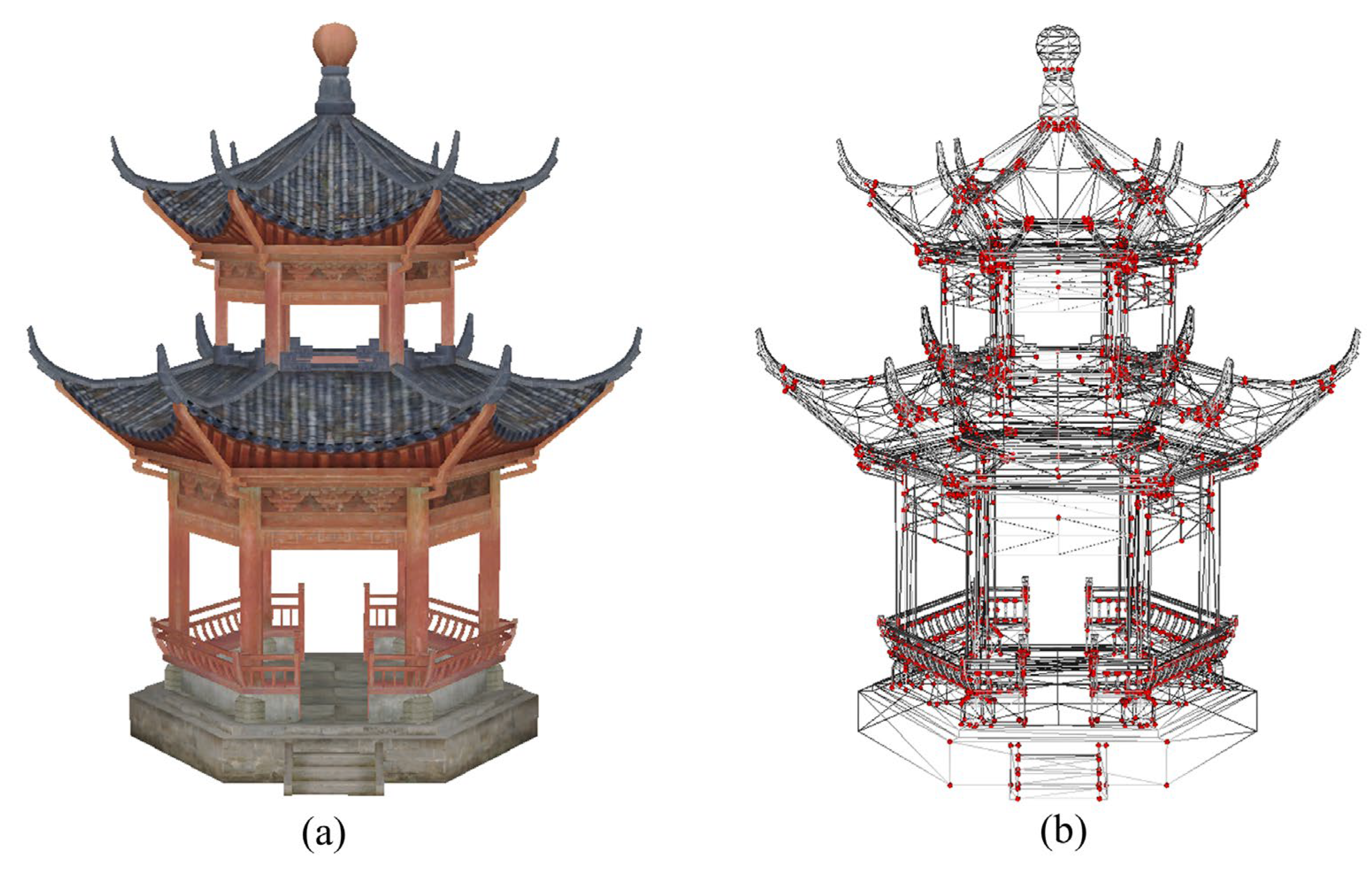
Figure 12.
Extraction result: (a) the original model; (b) the result (the red vertices are boundary vertices).
Figure 12.
Extraction result: (a) the original model; (b) the result (the red vertices are boundary vertices).

Figure 13.
E–C angle.

Figure 14.
Comparison of simplification results for the three building models: (a) the pavilion; (b) the apartment; (c) the house.
Figure 14.
Comparison of simplification results for the three building models: (a) the pavilion; (b) the apartment; (c) the house.

Figure 15.
Results of the user study: (a) the pavilion; (b) the apartment; (c) the house.

Figure 16.
Experiences of parameter analysis: (a) complex building (pavilion); (b) simple building (apartment).
Figure 16.
Experiences of parameter analysis: (a) complex building (pavilion); (b) simple building (apartment).

Figure 17.
Results of visibility analysis: (a) the original model; (b) the simplified model of the QEM method; (c) the simplified model of the proposed method. The location of the person is the viewpoint, and the light blue fan-shaped area represents the view. The visible buildings using the original model for visibility analysis are marked in blue. In addition, the difference in visible buildings between the model generated by the other methods and the original model is marked in red.

Figure 18.
Visualization of 3D city scenes from the street perspective: (a) QEM method; (b) the proposed method.
Figure 18.
Visualization of 3D city scenes from the street perspective: (a) QEM method; (b) the proposed method.


Table 1.
Simplification statistics for the three building models.
| Model | Number of Triangles | Number of Components | Number of Vertices | Simplification Rate | a | ||||
|---|---|---|---|---|---|---|---|---|---|
| Original | Simplified | Original | Simplified (QEM/ Chen’s/Ours) | Original | Simplified (QEM /Chen’s/Ours) | Boundary | |||
| Pavilion | 5752 | 2300 | 275 | 212/186/170 | 4060 | 2310/2218/2154 | 2510 | 60% | 2.0 |
| Apartment | 2567 | 513 | 103 | 53/47/57 | 1647 | 620/597/644 | 294 | 80% | 1.5 |
| House | 4428 | 2214 | 129 | 71/65/78 | 2317 | 1107/1053/1193 | 853 | 50% | 5.0 |
Table 2.
The detailed model information for parameter analysis.
| Model | Type | Simplification Rate | a |
|---|---|---|---|
 | complex | 60% | 2.0 |
 | complex | 70% | 3.8 |
 | complex | 50% | 5.0 |
 | simple | 80% | 1.5 |
 | simple | 80% | 1.6 |
 | simple | 70% | 2.6 |
 | simple | 70% | 2.0 |
Publisher’s Note: MDPI stays neutral with regard to jurisdictional claims in published maps and institutional affiliations. |
© 2021 by the authors. Licensee MDPI, Basel, Switzerland. This article is an open access article distributed under the terms and conditions of the Creative Commons Attribution (CC BY) license (https://creativecommons.org/licenses/by/4.0/).
Share and Cite
MDPI and ACS Style
Wang, B.; Wu, G.; Zhao, Q.; Li, Y.; Gao, Y.; She, J. A Topology-Preserving Simplification Method for 3D Building Models. ISPRS Int. J. Geo-Inf. 2021, 10, 422. https://0-doi-org.brum.beds.ac.uk/10.3390/ijgi10060422
AMA Style
Wang B, Wu G, Zhao Q, Li Y, Gao Y, She J. A Topology-Preserving Simplification Method for 3D Building Models. ISPRS International Journal of Geo-Information. 2021; 10(6):422. https://0-doi-org.brum.beds.ac.uk/10.3390/ijgi10060422
Chicago/Turabian StyleWang, Biao, Guoping Wu, Qiang Zhao, Yaozhu Li, Yiyuan Gao, and Jiangfeng She. 2021. "A Topology-Preserving Simplification Method for 3D Building Models" ISPRS International Journal of Geo-Information 10, no. 6: 422. https://0-doi-org.brum.beds.ac.uk/10.3390/ijgi10060422
Note that from the first issue of 2016, this journal uses article numbers instead of page numbers. See further details here.