Article

Characterizing the Up-To-Date Land-Use and Land-Cover Change in Xiong’an New Area from 2017 to 2020 Using the Multi-Temporal Sentinel-2 Images on Google Earth Engine

1
Heilongjiang Institute of Geomatics Engineering, Harbin 150081, China
2
College of Agronomy, Inner Mongolia Agricultural University, Hohhot 010019, China
*
Author to whom correspondence should be addressed.
ISPRS Int. J. Geo-Inf. 2021, 10(7), 464; https://0-doi-org.brum.beds.ac.uk/10.3390/ijgi10070464
Submission received: 28 April 2021 / Revised: 24 June 2021 / Accepted: 3 July 2021 / Published: 7 July 2021

Abstract

:
Land use and land cover (LULC) are fundamental units of human activities. Therefore, it is of significance to accurately and in a timely manner obtain the LULC maps where dramatic LULC changes are undergoing. Since 2017 April, a new state-level area, Xiong’an New Area, was established in China. In order to better characterize the LULC changes in Xiong’an New Area, this study makes full use of the multi-temporal 10-m Sentinel-2 images, the cloud-computing Google Earth Engine (GEE) platform, and the powerful classification capability of random forest (RF) models to generate the continuous LULC maps from 2017 to 2020. To do so, a novel multiple RF-based classification framework is adopted by outputting the classification probability based on each monthly composite and aggregating the multiple probability maps to generate the final classification map. Based on the obtained LULC maps, this study analyzes the spatio-temporal changes of LULC types in the last four years and the different change patterns in three counties. Experimental results indicate that the derived LULC maps achieve high accuracy for each year, with the overall accuracy and Kappa values no less than 0.95. It is also found that the changed areas account for nearly 36%, and the dry farmland, impervious surface, and other land-cover types have changed dramatically and present varying change patterns in three counties, which might be caused by the latest planning of Xiong’an New Area. The obtained 10-m four-year LULC maps in this study are supposed to provide some valuable information on the monitoring and understanding of what kinds of LULC changes have taken place in Xiong’an New Area.

1. Introduction

Land-use and land-cover (LULC) maps, such as impervious surface, vegetation, and waterbody, provide some fundamental description of the Earth’s land surface [1,2,3]. Timely and accurate acquisitions of LULC maps help to understand the development and progression of human society and contribute to the better modeling of climate and environmental change [4,5], thus playing an increasingly important role in modern society.
How to obtain the spatially explicit LULC maps with the least possible delay has become one of the pursuits in scientific communities, and a large number of research efforts have been exerted to achieve this goal. With the rapid development and advancement of remote sensing (RS) techniques, it has been gradually served as the main tool for researchers to obtain the LULC maps since RS techniques, in comparison to other traditional surveying and mapping approaches, possess the advantages of repeated observations and wide coverage, which suggests the high efficiency [6,7,8]. For example, the LULC changes and climate variation in the Three Gorges Reservoir catchment in China from 2000 to 2015 were analyzed and revealed using the GlobeLand30 data and Landsat 8 Operational Land Imager (OLI) images [4]. The impact of LULC change on meteorology in the Beijing-Tianjin-Hebei region of China from 1990 to 2010 was assessed and found that the temperature increase in the 2000–2010 period was greater than that in the 1990–2000 period mainly due to the transformation from croplands to urban and built-up lands [8]. The annual LULC maps in the conterminous United States from 1973 to 2000 was generated, and the changing patterns were summarized in that an almost 8.6% of the United States’ land area experienced a change in LULC at least one time [7]. It can be easily noted from these case studies that long time-series LULC maps were generated using RS images and then applied to unravel the mysterious masks of what the Earth’s land surface had undergone and what potential impact these changes might subsequently bring. Generally, machine-learning methods have played a significant role in these LULC studies, especially in accelerating the processing of a large volume of image stacks and in mining the unique patterns and knowledge related to the subsequent LULC changes. Furthermore, in order to obtain the LULC maps with more details and higher accuracy, the satellite images with better spectral, spatial, and temporal resolutions have been more and more applied, and a typical case of this obvious progress is to substitute the 500- or 250-m MODIS images with 30-m Landsat images and then 10-m Sentinel-2 images.
Since April 2017, the Xiong’an New Area, another state-level new area, was established in Hebei Province, North China [9,10]. Adjacent closely to Beijing and Tianjin, the newly established area is planned and expected to serve as an important component of the Beijing-Tianjin-Hebei metropolitan area as well as a region of non-capital core functions of Beijing [9]. It is foreseeable that akin to other state-level new areas, such as the Pudong New Area in Shanghai metropolis, a brand-new city will appear in Xiong’an. Although it is exciting to witness the development of Xiong’an New Area, it also poses the challenges of fully evaluating and understanding the development and impact of this new change. Among these challenges, one direct and obvious challenge is to explicitly monitor the LULC changes and evaluate the corresponding impact in Xiong’an New Area, as the newest development plan is supposed to bring dramatic changes in LULC types.
Several research studies have been made in recent years to obtain the LULC maps and to address the related changes in Xiong’an [11,12,13,14,15,16]. The LULC map of Xiong’an New Area, composed of impervious surface, vegetation, and water in 2016, was generated and used to predict the potential population growth and area expansion [12]. The impact of LULC change on the ecosystem from 1980–2015 in Xiong’an New Area was evaluated using the Landsat images [14]. The land-cover changes of Xiong’an in three discrete years, namely, in 2009, 2013, and 2017, were generated using the Landsat-5/8 images [16]. Though these LULC maps and research efforts have been made, it can be easily found that there were some limitations in the existing studies. First, previous studies focused on some limited land-cover types like surface water, which can only provide some information on how the selected limited classes changed. Second, a large number of studies were carried out before the establishment of Xiong’an New Area, thereby not providing the updated information on the LULC changes. Last, the coarse resolution images, such as MODIS or Landsat images, were usually applied in the existing studies, so the resultant LULC maps were more or less influenced by the mixed-pixels issues, thus leading to some uncertainties of analysis. As a result, it is of significance to find an effective way to generate the up-to-date LULC maps in Xiong’an New Area with fine spatial details and analyze the spatio-temporal change patterns of LULC types by overcoming these aforementioned limitations. Besides, there is no research that studies the varying developing patterns and speed in the three counties of Xiong’an New Area.
With the rapid development of cloud-computing methods, some powerful cloud-computing platforms have been developed to accelerate the monitoring of LULC maps. Among these developed platforms, the Google Earth Engine (GEE) has served as a new tech-tool to carry out some innovative studies [17,18,19]. In addition to the large volume of various long-term satellite observations, it also equips with some versatile classification models, such as the random forest (RF) [20,21,22,23] and support vector machine (SVM) [24,25,26], which makes it possible and efficient to carry out continuous monitoring of LULC maps. A huge number of research efforts have been conducted on GEE, such as global urban land extraction [27], global surface water monitoring [28], rice extraction [29], mangrove mapping [30], and land-cover mapping with 10-m Sentinel-2 images [31,32,33]. These research efforts have suggested the powerful computational ability and massive storage of GEE, which helps to achieve the fast and timely monitoring of LULC changes.
In light of this, this study used an efficient and effective method to extract the LULC maps in Xiong’an New Area with the multi-temporal 10-m Sentinel-2 images, which was deployed on the cloud-computing GEE platform. To do so, a novel multiple RF-based classification framework was proposed by outputting the classification probability based on each monthly composite and aggregating the multiple probability maps to generate the final classification map. Different from limiting to one specific year and in order to fully assess the spatiotemporal changes, the multi-year LULC maps in Xiong’an New Area from 2017 to 2020 were generated. This study then systematically evaluated the characteristics of the temporal and spatial LULC changes based on the annually generated LULC maps. We also estimated the performance of the obtained LULC map by comparing it with some previous land-cover maps of Xiong’an New Area. Overall, the resultant LULC maps were expected to provide basic information to evaluate the changing patterns, city planning, and some other issues, such as environmental protection, for the sustainable development of Xiong’an New Area.

2. Materials and Methods
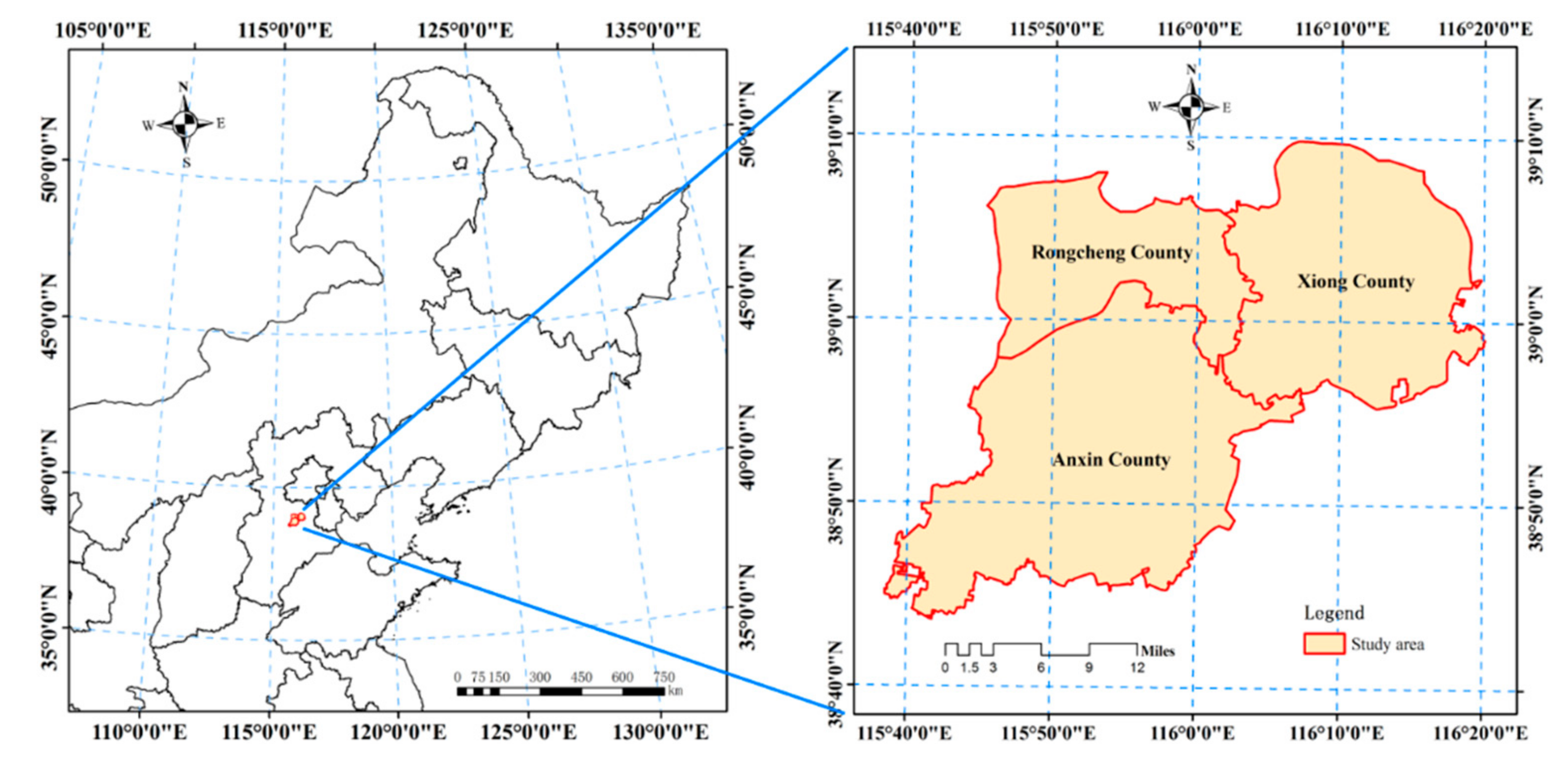
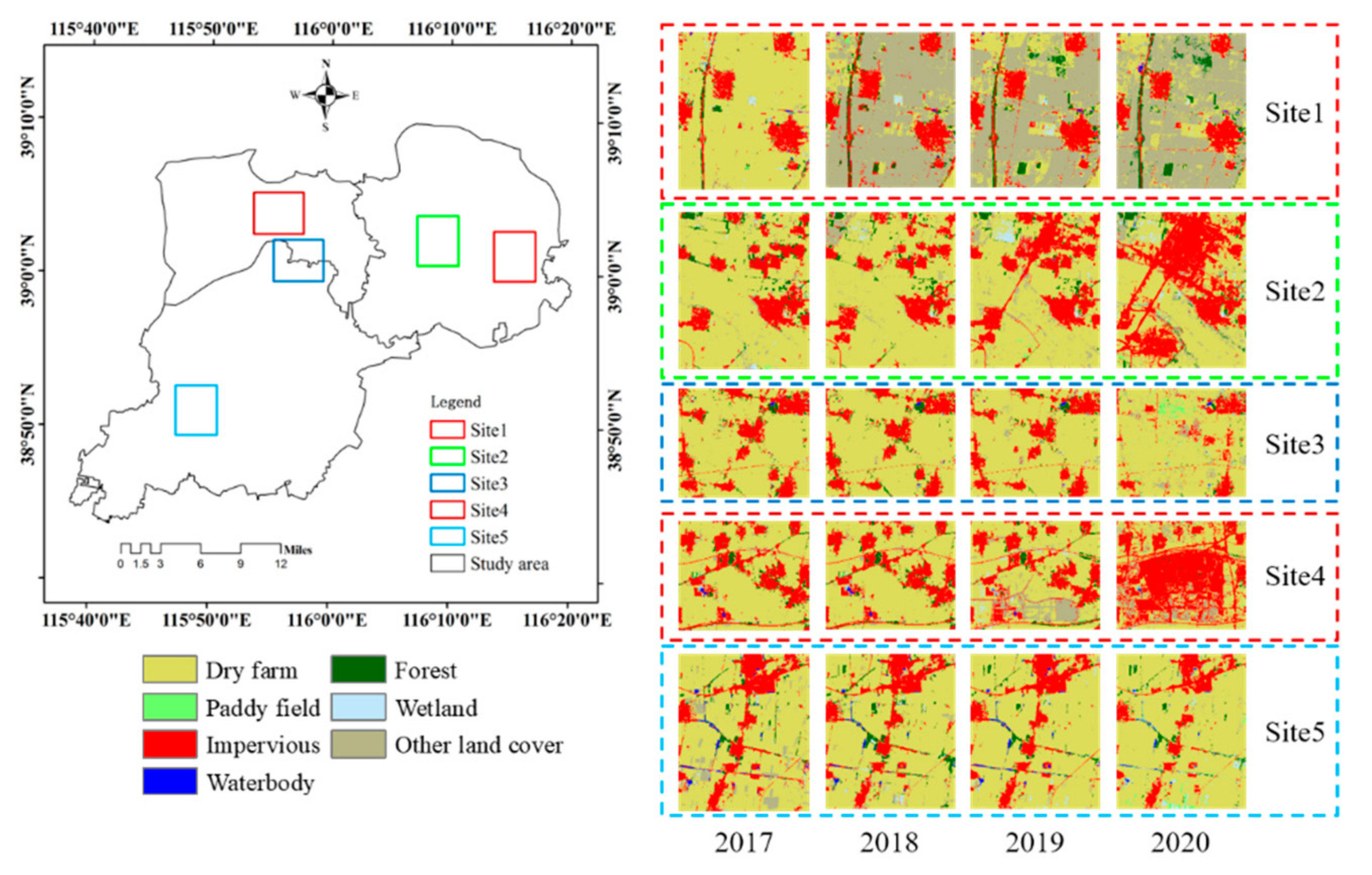
2.1. Study Area

The Xiong’an New Area was established on 1 April 2017. It is located at 38.92~39.06° N, 115.86~116.10° E in Hebei Province, China, mainly covering three counties, Xiong County, Anxin County, and Rongcheng County, and some surroundings adjacent to three selected counties, with an approximately planned 100 km2 at the initial stage, as shown in Figure 1. The predominant land cover is farmland, with Baiyangdian Lake, the largest lake in the North China Plain, covering its greatest portion in the south-central part, thus rich in water resources. The agricultural fields in Xiong’an New Area are large-size and flat, with dry farmland generally cultivated with wheat and corn in rotation. The wheat is normally harvested in June, and corn is grown from July to October, while the paddy fields grow rice from May to October. Belonging to the warm temperate monsoon continental climate, Xiong’an has an average annual temperature of 12.1 °C and average annual rainfall of 560 mm [9].

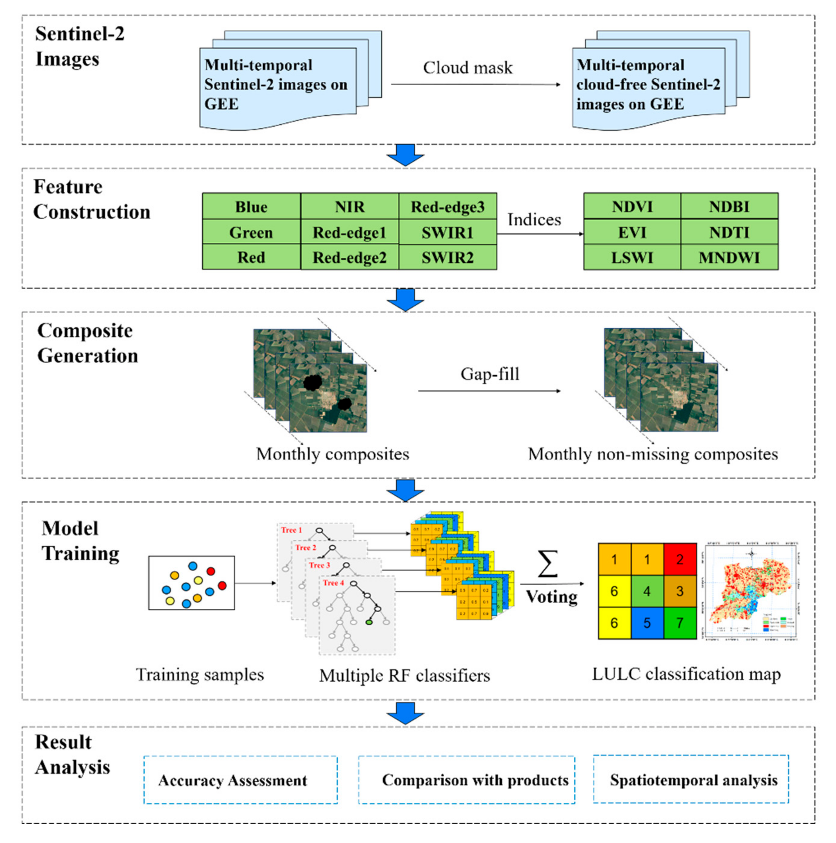
2.2. Satellite Imagery and Derived Vegetation Indices

The data used in this study were 10-m multi-temporal Sentinel-2 images data from 2017 to 2020, which was collected and well-organized on GEE [17]. The Sentinel-2 satellites were composed of two satellites, with the Sentinel-2A launched in 2015 and Sentinel-2B in 2017, that both had a 10-day revisit cycle [34]. The revisit cycle of two satellites combined can be further shortened to 5 days, thus providing dense, time-series observations. The multi-spectral imager (MSI) onboard took images at 13 different spectral bands, with a spatial resolution varying from 10 m to 60 m.
Considering the fact that not all Sentinel-2 images have been atmospherically corrected [35,36], the top of atmosphere (TOA) reflectance of Sentinel-2 images that belonged to Level 1C were used in this study. Additionally, due to the influence of cloud cover and summer rainfall, this paper used cloud percent <10% to filter the available data using the QA60 band. All Sentinel-2 images from June to September were collected and employed for LULC extraction.
In order to enhance the classification accuracy, six discriminative indices derived from the original bands were also computed, including normalized difference vegetation index (NDVI) [37], normalized difference building index (NDBI) [38], normalized difference tillage index (NDTI) [39], land surface water index (LSWI) [40], modified normalized difference water index (MDNWI) [41], and enhanced vegetation index (EVI) [42]. The mathematical expression of each vegetation index was provided as follows:
N D V I = N I R R e d N I R + R e d
N D B I = S W I R 1 N I R S W I R 1 + N I R
N D T I = S W I R 1 S W I R 2 S W I R 1 + S W I R 2
L S W I = N I R S W I R 1 N I R + S W I R 1
M N D W I = G r e e n S W I R 1 G r e e n + S W I R 1
E V I = 2.5 × N I R R e d N I R + 6 × R e d 7.5 × B l u e + 1
where Blue, Green, Red, NIR, and SWIR1 refer to the band 2,3,4,8, and 11, respectively.
In order to further mitigate the cloud contamination and also to reduce the computational burden, the monthly mean composites were generated. It was found that even using the monthly composite, there remained some places sabotaged by clouds. To handle this issue, we gap-filled missing pixels (cloud contaminated) with an interpolation filter by setting the mean value of the adjacent acquisitions. If a pixel was contaminated with clouds in the monthly mean composite, the following method would be used to reconstruct a pixel value; otherwise, its original value was maintained.
d t = m e a n   [ d t 1 , d t + 1 ]
where d t was the observed pixel at time t, and mean was the mean function to obtain the average values of two adjacent images.

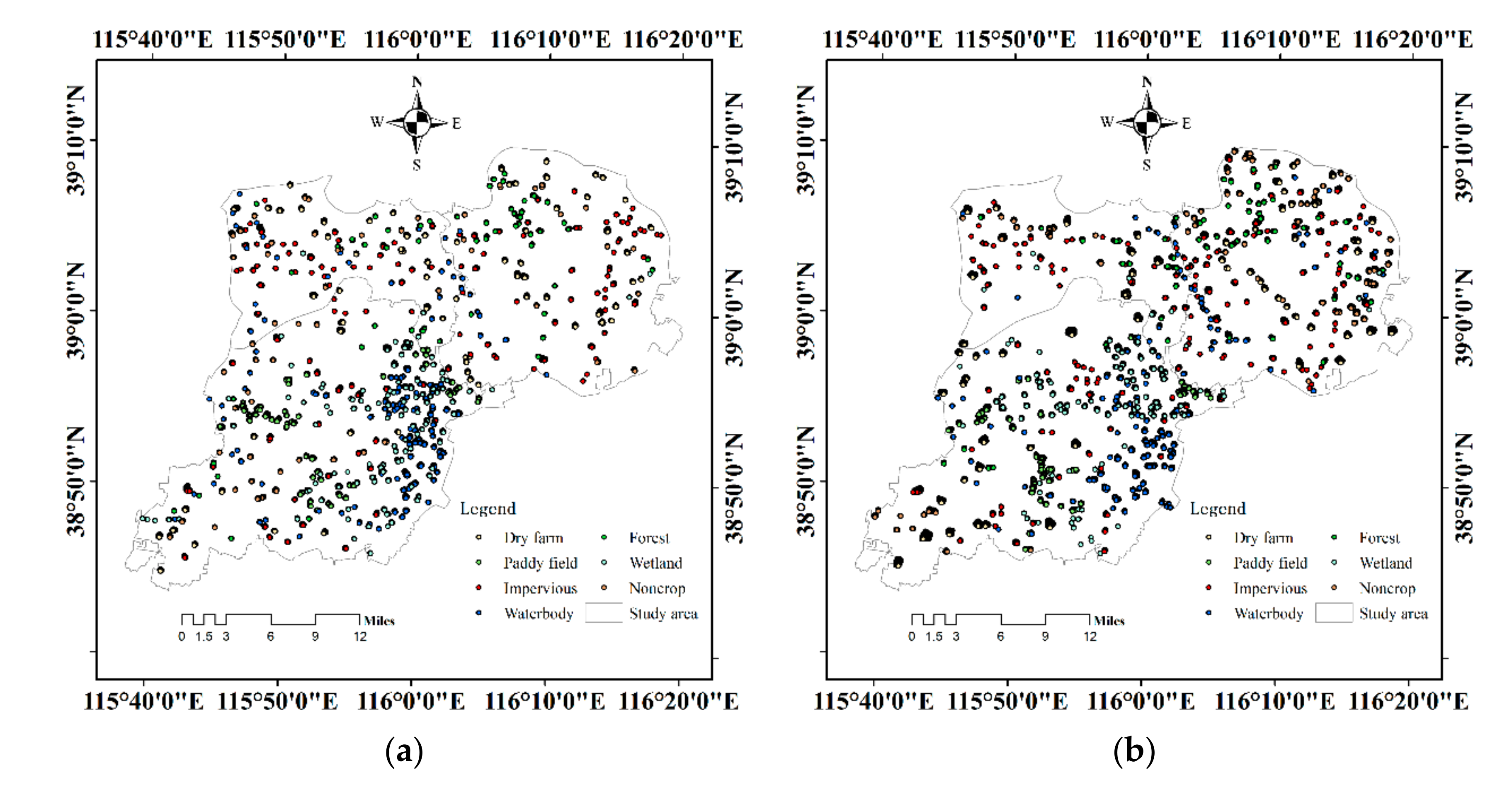
2.3. Training and Validation Sample Data

In this study, reference sample data was interpreted and collected by combining careful visual interpretation of mulita-temporal Sentinel-2 images and Google Earth high-resolution images. On consideration of the existing LULC types in Xiong’an, a total number of 7 classes were, at last, selected to describe the spatiotemporal variations of LULC in Xiong’an, including dry farmland, paddy field, the impervious surface, waterbodies, forest, wetland, and other land, as listed in Table 1. For each year, more than 70,000 samples were collected. For example, the spatial distributions of collected reference samples in 2017 and 2019 were given in Figure 2. For the selected sample data, 70% were used for training the classification model, and the remaining 30% were used for accuracy testing.

2.4. Methodology

In this study, the classification task is employed on the GEE platform, which is mainly composed of cloud-free image generation, vegetation indices computation, monthly mean composite generation, missing-data filling, random forest classification model training, and accuracy assessment. The overall classification flowchart is shown in Figure 3. As the Sentinel-2 images are easily contaminated by clouds, the first step is to mask out cloud pixels using the QA60 band [43,44]. Then, the six selected indices are computed to enhance the discriminative characterizations of different land covers. After that, the monthly mean composites for the nine original spectral bands and six indices are derived in order to further mitigate the negative impact of cloud contamination and to reduce computational complexity. To avoid the missing data, the obtained composites are further gap-filled using the Equation (7) introduced in Section 2.3. Following that, the random forest (RF) classifier is chosen to implement the LULC classification task by feeding the collected sample data and derived feature collections. Finally, the multi-year LULC maps from 2017 to 2020 are obtained and used to analyze spatio-temporal LULC changes in Xiong’an New Area.
Random forest (RF) belongs to one member of the ensemble learning family, possessing the advantages of high accuracy, good robustness, and easy parameterization [20,21]. An RF classifier is generally composed of a large number of base weak classifiers, each of which is an independent individual classification and regression tree (CART). The RF-based model has been widely employed in RS communities and applied in various LULC classification tasks [22,45,46,47]. To implement the RF, two fundamental parameters are needed in an RF: one is the number of trees (ntree) for constructing a whole forest, and the other is the number of picked features (mty) that are used for node splitting.
Differing from the existing studies, multiple RF models based on the monthly composites are applied in this study to carry out classification, as shown in Figure 3. For each RF, instead of directly outputting the classification class, it is set to produce the classification probability of each class, say seven class probability in our study. We then aggregate the four class probability maps into one final probability map and set a class with the largest maximum probability as the final class. In doing so, it possesses two advantages over the traditional usage of RF models. First, it is based on each monthly composite, thus having less computational cost. Second, we change the hard classification into soft classification, which is more suitable for multi-classification problems. To the best of our knowledge, the adopted soft-classification strategies have been rarely utilized in the previous studies, at least not very often on GEE. For each RF, nine original bands (band 2–8 and band 11–12) and six derived indices (9 × 5 + 6 × 5) are used as the classification features. The mty variable is, as suggested in the existing literature, calculated as the square root of the number of input features [20,21]. For the parameter of ntree, we test different numbers, ranging from 20 to 500, and finally set to 100 as stable performance is achieved.

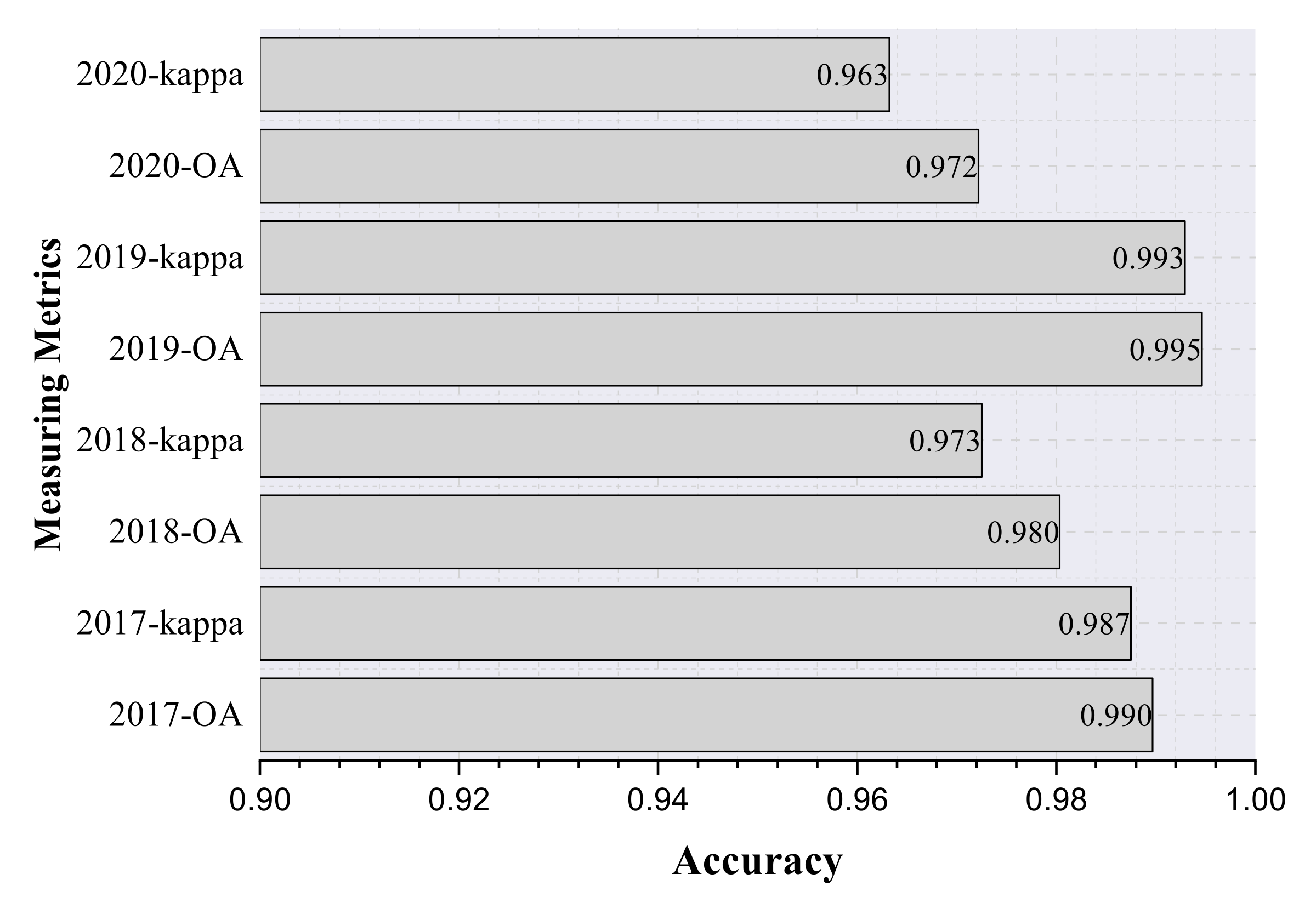
2.5. Accuracy Assessment of the Derived LULC Maps

In this study, the collected samples were employed to compute the confusion matrix for each LULC map, and the widely used measuring metrics, such as the overall accuracy (OA) and Kappa coefficient, were calculated to assess the proposed method and the derived LULC maps [48,49,50].

2.6. Comparisons with the Availble Products

In this study, we also collected some available products in Xiong’an New Area as the reference to assess the accuracy and performance of our LULC maps. The dataset of annual global impervious surface areas from 1985 to 2018 with a spatial level of 30 m was generated using a combined approach of supervised classification and temporal consistency checking [51]. The impervious pixels in [51] are defined as above 50 percent impervious, mainly composed of urban areas and some road infrastructures. The impervious surface area of each year can be obtained using the transition numbers. For example, the impervious surface in 2018 can be generated as the pixel value greater than 1 [51], which has been included on the GEE platform. In this study, the 30-m impervious surface area of Xiong’an New Area in 2017 and 2018 are downloaded as the reference.

3. Results and Discussion

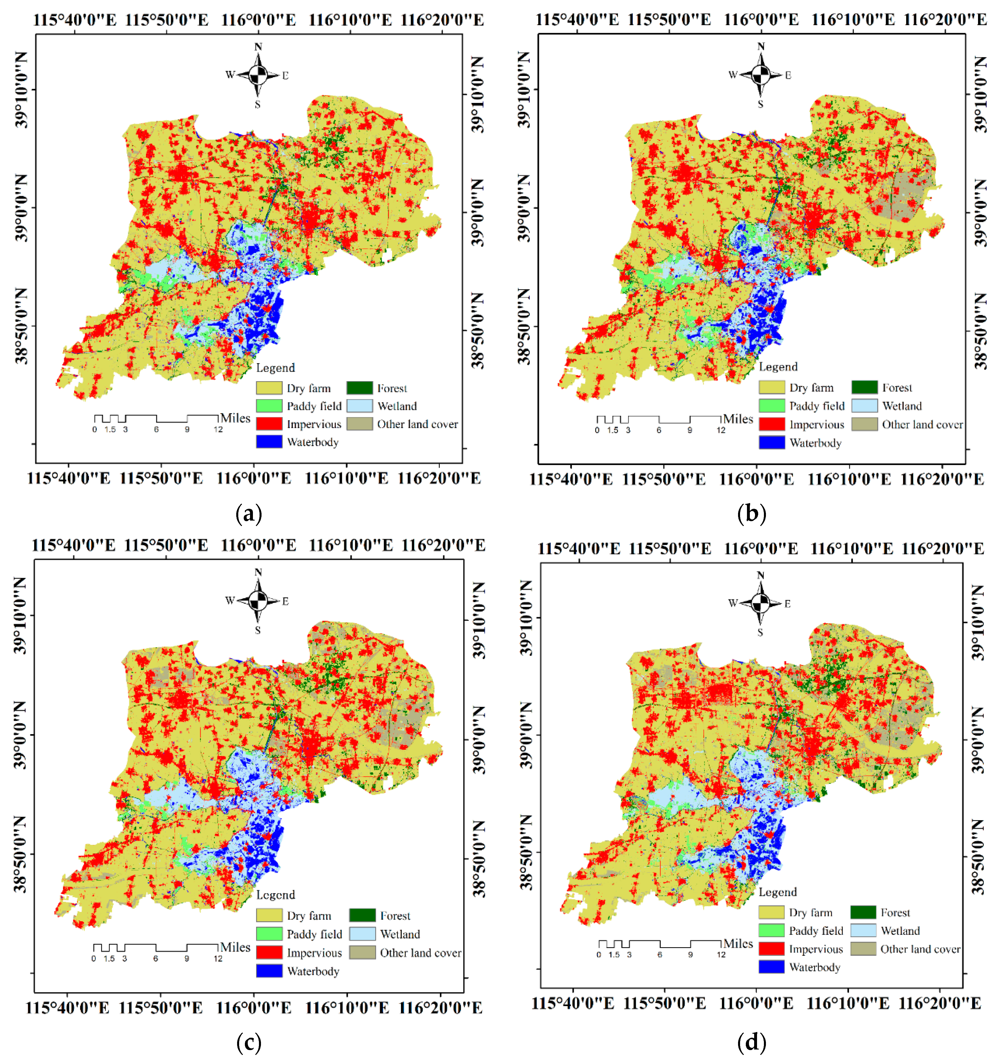
3.1. The Distribution Maps of LULC in Xiong’an New Area and Accuracy Assessment and Change of Land Use

The LULC thematic maps in Xiong’an New Area from 2017 to 2020 are presented in Figure 4. It can be seen that Xiong’an New Area is rich in arable land resources of which dry farmland accounts for the majority, and paddy fields are concentrated in the central and southern regions, close to water bodies. This is also in line with the distribution characteristics of paddy fields, as paddy fields depend on water sources, so they are concentrated near lakes or rivers that can provide sufficient irrigation for paddy rice growing. A rough comparison shows that residential areas and other architectural areas show a certain degree of expansion. Noticeably, since 2018, a large portion of other land cover is shown, in particular in the Northeast region of Xiong’an New Area. In order to better characterize the LULC distribution patterns in Xiong’an New Area, we document the changed areas and unchanged LULC types, shown in Figure 5. It is clearly shown in Figure 5 that a large portion of areas has been changed, particularly in the northern regions. The changed areas are calculated and found to account for nearly 36 percent of Xiong’an New Area, indicating that intensive changes are undergoing in the study area.
The LULC maps in Xiong’an New Area from 2017 to 2020 are measured using the collected reference samples, and the OA and Kappa values for each year are obtained, as shown in Figure 6. It can be seen that for each year, the OA and Kappa values are both higher than 0.95, indicating that the proposed method achieves high performance, and our multi-temporal-based mapping results are highly accurate. The derived high-accuracy LULC maps are then employed to evaluate the spatial and temporal changes in Xiong’an New Area.

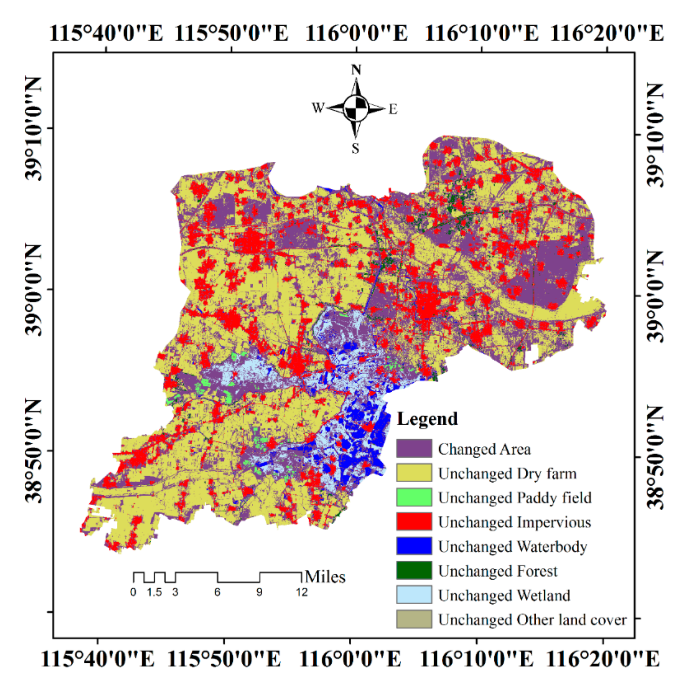
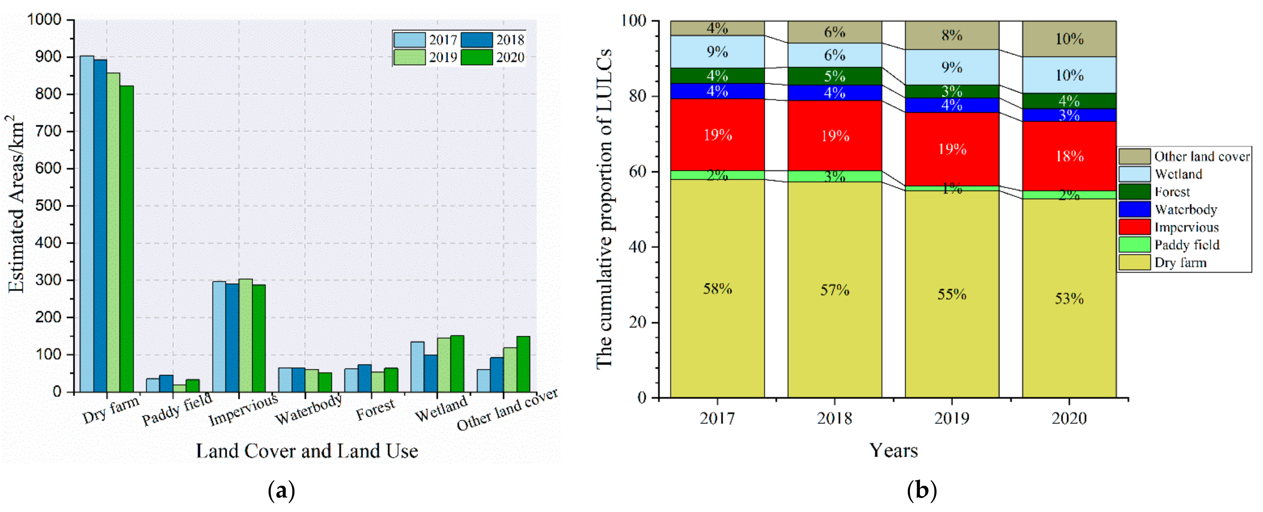
3.2. The Spatiotemporal Changes and Patterns of LULC in Xiong’an New Area from 2017 to 2020

In order to further and quantitatively evaluate and compare the spatial and temporal changes of different LULC types in Xiong’an New Area, the estimated areas and the cumulative ratio for each class from 2017 to 2020 are computed and presented in Figure 7. Several interesting findings are revealed in Figure 7. First, it is clearly shown that the dry farmland gradually decreased since 2017 and the area proportions reduced from 58% to 53%. The other land-cover class has increasingly grown from 2017, and the corresponding area proportions increased from 4% to 10%, which is also exhibited in Figure 4. We carefully checked the images and classification results and found that since 2018, Xiong’an New Area has increased the investment in landscape and ecology, and some regions are specially designed as tree seedlings and landscape dual-use regions. As it is different from forests and other landscapes, it is provisionally categorized as the other land-cover class in this study. The most novel finding of the LULC changes comes from the impervious class, which is mainly composed of buildings and road facilities that are basically human-made. Interestingly, the impervious surface first decreased from 2017 to 2018 and then increased in 2019, and finally decreased in 2020. This unique phenomenon in estimated impervious areas seems to imply that the development of Xiong’an New Area is not just an expansion of the building areas, which is of interest to the existing studies. Other LULC types, such as wetlands, paddy fields, and forest, also show some variations.
Five sites in Xiong’an New Areas were selected to further demonstrate the spatio-temporal LULC changes, as shown in Figure 8. Except for site 5, which showed minor inter-annual changes, the other four sites clearly exhibited dramatic changes since the establishment of Xiong’an New Area. Specifically, for site 1, the dry farmland has shifted to other land cover since 2018 and undergone small variations after that. This site was planned as a region for tree seedlings and landscape dual-use. For site 2, there were no major changes during 2017–2018 period, but in 2019 and 2020, the majority of this site shifted from dry farmland to impervious types, which mainly included buildings, two high-speed ways, and a newly built residential area. Actually, the north region was where Xiong’an Station is located. From our mapping results, it can be concluded that the station was successfully built within nearly one year. For site 3, it can be noticed that the impervious areas shrunk, mainly starting from 2019, and in 2020, this site was almost completely changed into dry farmland. Contrarily, a brand-new building agglomeration is now shown on site 4. On consideration of the geographical adjacency to each other, it stands a good chance that the people in site 3 moved toward site 4, thus generating the concentration effect. We argue that this intensified relocation project is one of several big plans in Xiong’an New Area to optimize the allocation of resources. This meticulous analysis and comparison here might explain why the impervious surface in Xiong’an New Area first increased and then decreased, as revealed in Figure 7. Apparently, the increase of impervious surface largely comes from the constructions of urban areas, including new business centers and transportation facilities, such as the aforementioned Xiong’an New Station. The loss of impervious surface is possibly due to the demolition of rural houses based on the newest planning, such as township transformation to new aggregation city.
From the above analysis, it was clearly revealed that after the establishment of Xiong’an New Area in 2017, the LULC types in both spatial and temporal dimensions underwent dramatic changes. For instance, the Xiong’an station was successfully established in 2009–2020, and additionally, some villages were removed and relocated to other regions, such as in sites 3 and 4. These changes will be further revealed in the future.

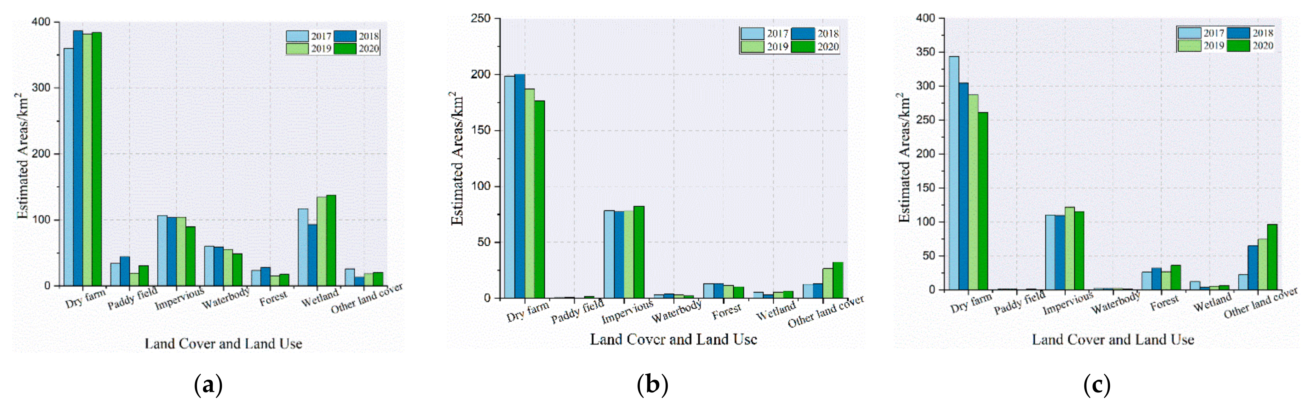
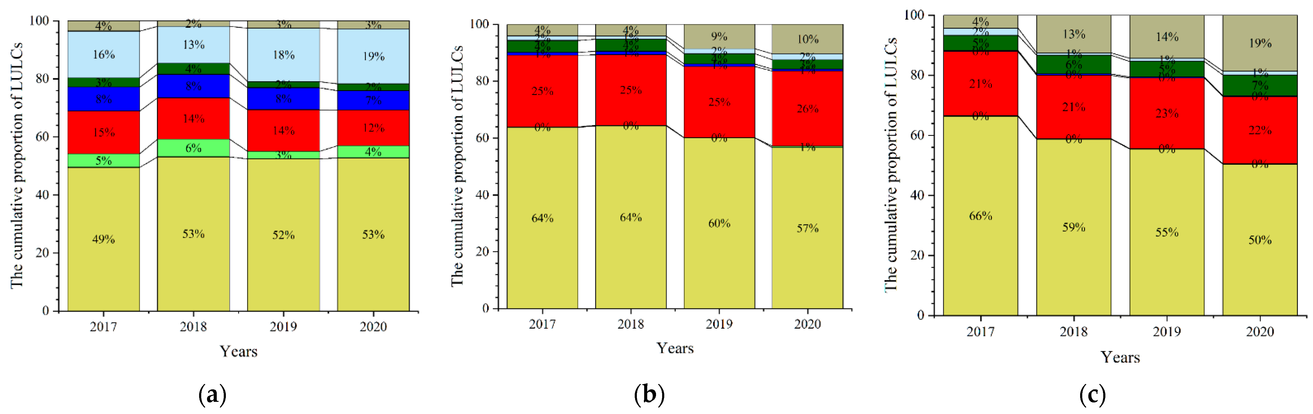
3.3. Assessment of the Different LULC Changing Patterns of Three Counties in Xiong’an New Area

As Xiong’an New Area is mainly composed of three counties, we here want to know whether the LULC changing patterns or changing speed of these three counties are similar or different. We compute the estimated areas from 2017 to 2020 of each LULC type in each county, as shown in Figure 9. Accordingly, the area proportion of each class from 2017 to 2020 is also calculated in Figure 10.
It can be seen in Figure 9 and Figure 10 that the estimated LULC types of these three counties present varying characteristics. The dry farmland in Rongcheng County and Xiong County shows decreased trends, while the dry farmland in Anxin County has increased, which exhibits the opposite trends for other land cover. As discovered in Figure 4 and Figure 5, the dry farmland areas for both Rongcheng County and Xiong County decreased due to the planning of establishing the dual-use regions of the tree seedlings and landscape, while in Anxin, almost no similar regions were detected. Particularly, the area proportions of other land cover in Rongcheng County and Xiong County increased from 4% to 10% and 19%, respectively. For the impervious surface, the estimated areas in Anxin County decreased in a general sense, while in Rongcheng and Xiong County, small changes were exhibited. This different phenomenon revealed in three counties might explain why the impervious surface in Xiong’an New Area presented variations instead of a continuous rise from 2017 to 2020.
In summary, the LULC maps in three counties present some varying characteristics, such as other land cover and impervious changes in three distinct counties, which is mainly caused by urban planning of different counties. This different analysis here provides some better planning and understanding of what kinds of changes are taking place in Xiong’an New Area, which might contribute to more effective and scientific decision-making in the future.

3.4. Comparisons among the Derived LULC Maps and Other Land-Cover Maps of Xiong’an New Area

Here, we compare the obtained 10-m Sentinel-2 derived LULC maps in this study and the 30-m Landsat impervious surface in terms of spatial patterns and estimated areas. The 30-m impervious surface maps are generated using the Landsat images, and the impervious surface maps in 2017 and 2018 are obtained, as shown in Figure 11, in combination with our 10-m Sentinel-2 impervious surface maps and the spatio-temporal change map.
It is observed from Figure 11 that the impervious surface maps from Sentinel-2 and Landsat in the corresponding years present similar spatial distribution patterns, implying that the impervious surface maps generated in this study have high confidence. Different from the 30-m Landsat impervious surface maps, our impervious surfaces have a higher spatial resolution, thus exhibiting more spatial details. We also compute the areas of impervious surface based on these two products as listed in Table 2 and only found some minor differences. For example, the estimated areas of impervious surface in 2017 from the Landsat and Sentinel-2 are 312.64 km2 and 296.03 km2, respectively, with around 5 percentage error in total, which shows high-value consistency. Additionally, the 30-m Landsat-derived impervious areas are bigger than the impervious areas from 10-m Sentinel-2 images, which might be caused by the mixed pixels in the 30-m Landsat pixels. In Figure 11e, the spatio-temporal impervious surface changes based on our 10-m Sentinel-2 images are also revealed, where 0 and 1 denote non-impervious and impervious, respectively, and the number of digits signifies how many years are calculated. For example, “1,1,1,1”, “1,1,1”, ”1,1”, and “1” represent the impervious information for ‘’2017–2020”, “2018–2020”, “2019–2020”, and “2020”, respectively, and “1,1,1,0” indicates that before 2020, it is impervious surface, while in 2020, it changes into non-impervious; however, “0,0,1,1” suggests that before 2019, it is not impervious surface but becomes impervious surface after 2019. It is shown that most impervious regions stay stable in the last four years in Xiong’an New Area, but some dramatic changes are also observed, especially in the Rongcheng County and Xiong County. On the contrary, the impervious surface increase in Anxin County is not observed. These spatio-temporal changes are in accordance with Section 3.3, where the different patterns of LULC changes in three counties are described. The 30-m Landsat derived impervious surface products can also be used to carry out this kind of analysis, but it is limited to two years. Consequently, it cannot reveal more findings than are revealed through our four-year continuous impervious surface maps.

3.5. The Advantages and Limitations of the Proposed Approach

In this study, we made full use of the finer high resolution (10 m) and better temporal resolution (5 to 10 days) Sentinel-2 images on the cloud-computing GEE platform to extract the LULC maps of Xiong’an New Area from 2017 to 2020. The continuous-year LULC maps were, in a general sense, difficult to generate and obtain, which might lead to some misunderstanding of the subsequent analysis. For example, based on our derived LULC maps, it was interesting to find out that the impervious surface areas of Xiong’an New Area increased at first and then decreased, as revealed in Figure 7 and Figure 11. Based on the derived LULC maps, we first analyzed the spatio-temporal changes of LULC in Xiong’an New Area, and then we further evaluated the different development patterns in three counties and found that the LULC maps in three counties presented some varying characteristics. Different from some existing studies, our derived LULC maps have more land-cover types, finer spatial resolutions, and better inter-annual continuity, continually covering the years from 2017 to 2020. Although the improvement was revealed in our LULC maps, it should be pointed out that some difference was inherent from the varying spatial resolution of different satellite images. For instance, the 10-m Sentinel-2 presented more spatial details than the 30-m Landsat images. Actually, it was one of the main motivations in this study, as there were few studies that carried out the LULC classification in Xiong’an New Area with 10-m Sentinel-2 images, and this study was expected the fill in this gap.
In this study, we utilized the RF classifier to carry out the classification task. However, different from the traditional usage of the RF model in a large number of studies, multiple RF-based classification models based on the monthly composites were employed in this study. Instead of directly outputting the assigned classes, each RF produced seven probability maps for each class, and these probability maps were finally grouped to yield the final classification result. In doing so, the traditional hard classification was converted to soft classification, which might be more accurate, as the classification results can be further adjusted based on the classification confidence.
Apparently, the improved performance of this study was attributed to some significant aspects: First, the utilization of GEE made it possible to generate LULC maps in a very efficient way that cannot be applied in the past [17,31,52,53,54]. For example, the satellite images were processed using the client computers in the past, which was inconvenient and time-consuming even simply for the processing of images, such as atmospheric correction and mosaicking. However, on GEE, these processing steps have been handled in advance, thus significantly reducing the complexity in the entire process. Second, multi-temporal images were employed in this study. In comparison to the single-date image, the multi-temporal images can provide more complementary information to discriminate different land covers, thus having better classification accuracy. For example, the paddy field and dry farmland might be difficult to distinguish in July or August, but the rice was easy to distinguish from dry cropland in June due to the flooding signals of rice fields [29]. Additionally, we further gap-filled the missing data using the interpolation method, which was an effective means to handle the missing data caused by cloud or rainy contamination.
However, there exist some limitations or uncertainties in this study, which will be further considered in the future. First, the LULC changes are expected to dramatically take place in Xiong’an New Area so that some land covers, such as the impervious surface, might change even in a month. In this sense, even if multi-temporal images are employed, it cannot be accurate to monitor and characterize these dramatic changes. Second, the spectral features are solely applied in this study without posing more constraints, such as object-based analysis in the extraction of LULC coverage. As a result, the performance of LUC maps obtained in this study might be further improved by incorporating some more sophisticated approaches. These limitations will be further studied in our future research.

4. Conclusions

In this study, we used the 10-m multi-temporal Sentinel-2 images to monitor and analyze the continuous spatio-temporal changes of land use and land cover (LULC) in Xiong’an New Area from 2017 to 2020, which was implemented on the Google Earth Engine (GEE) cloud-computing platform. A novel multiple random forest model based on monthly composites was adopted in this study. The obtained LULC maps were fully evaluated using the geo-referenced sample data and other available land-cover maps. It can be observed that our derived, continuous LULC maps had more land types and better spatial details. Through the all-around comparison and analysis, it was found that the land-use types and areas of Xiong’an New Area in both temporal and spatial dimensions have been significantly changed and can be concluded as follows:
(1)
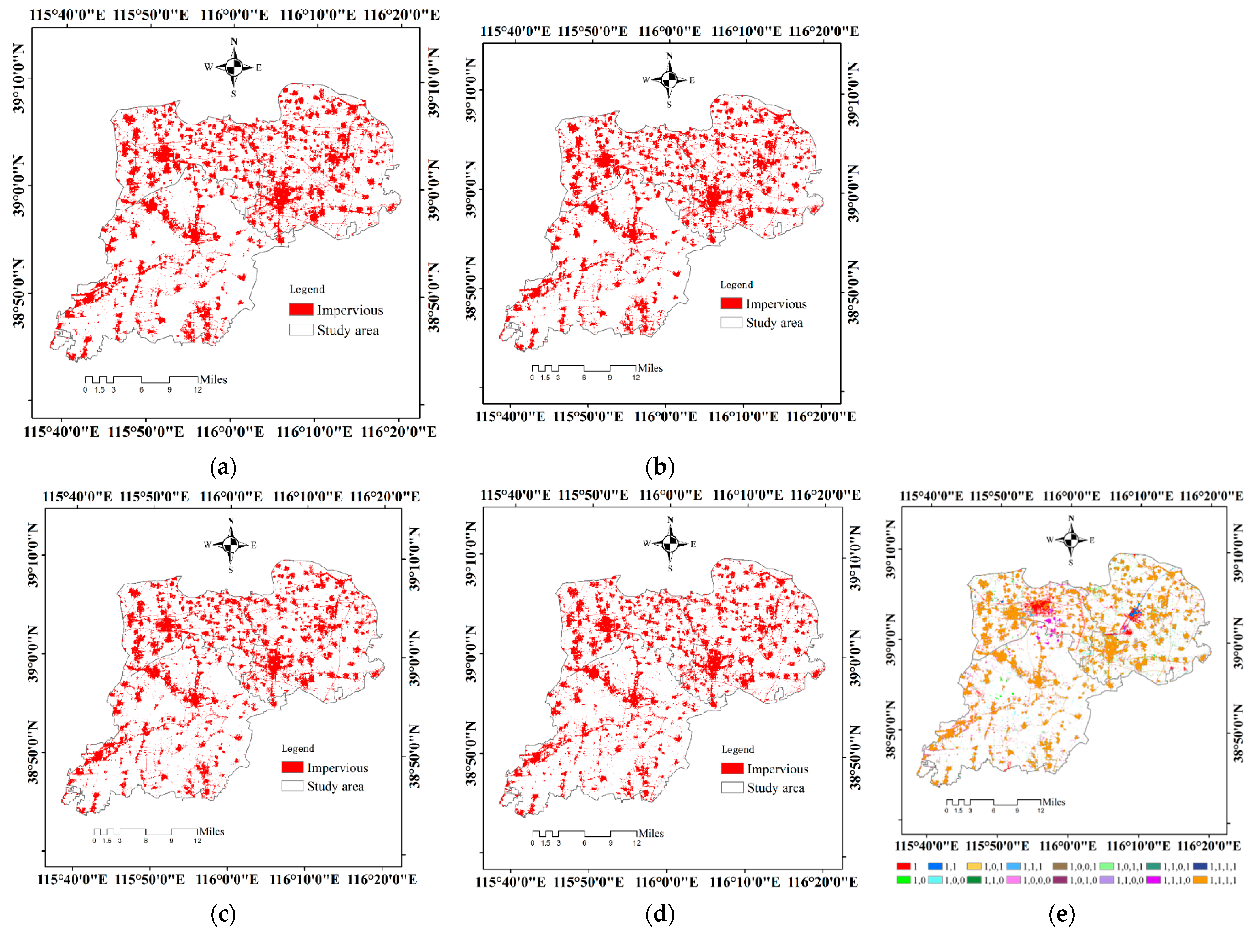
The impervious areas (mainly including the buildings and road infrastructure) in the recent four years first increased and then decreased. The increase was due to the construction of some infrastructure, such as the high-speed station and some overpasses and highways. The following decrease was mainly contributed to the housing relocation. Some small villages were dismantled and aggregated to the same places, thus forming bigger building groups.
(2)
The dry farmland decreased from 2017, with the majority of it in the northeastern part of Xiong’an New Area, converted to tree seedlings and landscape dual-use regions. As a result, the other land cover class dramatically increased, especially in the east of Xiong County.
(3)
It has been found in this study that the three main counties in Xiong’an New Area showed different development patterns. This different analysis was supposed to provide some better planning and understanding of what kinds of changes were undergoing in Xiong’an New Area.

Author Contributions

Conceptualization, Jiansong Luo and Xinwen Ma; Data curation, Jiansong Luo and Qifeng Chu; Formal analysis, Jiansong Luo, Xinwen Ma, Qifeng Chu, Min Xie and Yujia Cao; Funding acquisition, Xinwen Ma; Investigation, Jiansong Luo; Methodology, Jiansong Luo and Yujia Cao; Supervision, Xinwen Ma; Validation, Qifeng Chu, Min Xie and Yujia Cao; Writing—original draft, Jiansong Luo; Writing—review and editing, Jiansong Luo, Xinwen Ma, Qifeng Chu, Min Xie and Yujia Cao. All authors have read and agreed to the published version of the manuscript.

Funding

This work was supported by the Basic Surveying and Mapping Technology and Standard Program of 2020 (Phase I) of Heilongjiang Bureau of Surveying, Mapping Geographic Information under grant 202004.

Data Availability Statement

The data presented in this study are available from the lead author (J.L.) on request.

Acknowledgments

We offer our special thanks to the Google team for building the powerful Google Earth Engine (GEE) platform and providing free access and service to us, which helps us to develop our algorithm to extract the land cover in a timely and accurate manner. We are also grateful to the anonymous reviewers for their comments, which resulted in significant improvements to some parts of the manuscript.

Conflicts of Interest

The authors declare no conflict of interest.

References

  1. Saadat, H.; Adamowski, J.; Bonnell, R.; Sharifi, F.; Namdar, M.; Ale-Ebrahim, S. Land use and land cover classification over a large area in Iran based on single date analysis of satellite imagery. ISPRS J. Photogramm. Remote. Sens. 2011, 66, 608–619. [Google Scholar] [CrossRef]
  2. Zhu, Z.; Woodcock, C.E.; Rogan, J.; Kellndorfer, J. Assessment of spectral, polarimetric, temporal, and spatial dimensions for urban and peri-urban land cover classification using Landsat and SAR data. Remote Sens. Environ. 2012, 117, 72–82. [Google Scholar] [CrossRef]
  3. Ban, Y.; Gong, P.; Giri, C. Global land cover mapping using Earth observation satellite data: Recent progresses and challenges. ISPRS J. Photogramm. Remote Sens. 2015, 103, 1–6. [Google Scholar] [CrossRef] [Green Version]
  4. Hao, B.; Ma, M.; Li, S.; Li, Q.; Hao, D.; Huang, J.; Ge, Z.; Yang, H.; Han, X. Land Use Change and Climate Variation in the Three Gorges Reservoir Catchment from 2000 to 2015 Based on the Google Earth Engine. Sensors 2019, 19, 2118. [Google Scholar] [CrossRef] [Green Version]
  5. Kuang, W.; Yang, T.; Yan, F. Examining urban land-cover characteristics and ecological regulation during the construction of Xiong’an New District, Hebei Province, China. J. Geog. Sci. 2018, 28, 109–123. [Google Scholar] [CrossRef] [Green Version]
  6. Yu, M.; Guo, S.; Guan, Y.; Cai, D.; Zhang, C.; Fraedrich, K.; Liao, Z.; Zhang, X.; Tian, Z. Spatiotemporal Heterogeneity Analysis of Yangtze River Delta Urban Agglomeration: Evidence from Nighttime Light Data (2001–2019). Remote Sens. 2021, 13, 1235. [Google Scholar] [CrossRef]
  7. Sleeter, B.M.; Sohl, T.L.; Loveland, T.R.; Auch, R.F.; Acevedo, W.; Drummond, M.A.; Sayler, K.L.; Stehman, S.V. Land-cover change in the conterminous United States from 1973 to 2000. Glob. Environ. Chang. 2013, 23, 733–748. [Google Scholar] [CrossRef] [Green Version]
  8. Li, J.; Zheng, X.; Zhang, C.; Chen, Y. Impact of Land-Use and Land-Cover Change on Meteorology in the Beijing–Tianjin–Hebei Region from 1990 to 2010. Sustainability 2018, 10, 176. [Google Scholar] [CrossRef] [Green Version]
  9. Xu, H.; Shi, T.; Wang, M.; Fang, C.; Lin, Z. Predicting effect of forthcoming population growth–induced impervious surface increase on regional thermal environment: Xiong’an New Area, North China. Build. Environ. 2018, 136, 98–106. [Google Scholar] [CrossRef]
  10. Liu, Z.; de Jong, M.; Li, F.; Brand, N.; Hertogh, M.; Dong, L. Towards Developing a New Model for Inclusive Cities in China—The Case of Xiong’an New Area. Sustainability 2020, 12, 6195. [Google Scholar] [CrossRef]
  11. Song, C.; Ke, L.; Pan, H.; Zhan, S.; Liu, K.; Ma, R. Long-term surface water changes and driving cause in Xiong’an, China: From dense Landsat time series images and synthetic analysis. Sci. Bull. 2018, 63, 708–716. [Google Scholar] [CrossRef] [Green Version]
  12. Wang, Z.; Cao, J. Assessing and Predicting the Impact of Multi-Scenario Land Use Changes on the Ecosystem Service Value: A Case Study in the Upstream of Xiong’an New Area, China. Sustainability 2021, 13, 704. [Google Scholar] [CrossRef]
  13. Su, H.; Wang, W.; Jia, Y.; Han, S.-C.; Gao, H.; Niu, C.; Ni, G. Impact of urbanization on precipitation and temperature over a lake-marsh wetland: A case study in Xiong’an New Area, China. Agric. Water Manage. 2021, 243, 106503. [Google Scholar] [CrossRef]
  14. Wang, Z.; Cao, J.; Zhu, C.; Yang, H. The Impact of Land Use Change on Ecosystem Service Value in the Upstream of Xiong’an New Area. Sustainability 2020, 12, 5707. [Google Scholar] [CrossRef]
  15. Liu, S.; Cui, Y.; Li, N.; Deng, X.; Shi, X.; Liu, X.; Zhao, F. In the study of interannual change of urban expansion, precipitation and water area of baiyang lake in Xiong’an new area. In Proceedings of the 2018 26th International Conference on Geoinformatics, Kunming, China, 28–30 June 2018; pp. 1–4. [Google Scholar]
  16. Gao, P.; Wang, S.; Li, W.; Gao, X. Analysis of Spatial and Temporal Variation of Land Use in Xiong’an New Area Based on Re-mote Sensing Data. Available online: https://www.x-mol.com/paper/1376443291721510912?adv (accessed on 3 July 2021).
  17. Gorelick, N.; Hancher, M.; Dixon, M.; Ilyushchenko, S.; Thau, D.; Moore, R. Google Earth Engine: Planetary-Scale geospatial analysis for everyone. Remote Sens. Environ. 2017, 202, 18–27. [Google Scholar] [CrossRef]
  18. Kumar, L.; Mutanga, O. Google Earth Engine Applications since Inception: Usage, Trends, and Potential. Remote Sens. 2018, 10, 1509. [Google Scholar] [CrossRef] [Green Version]
  19. Tamiminia, H.; Salehi, B.; Mahdianpari, M.; Quackenbush, L.; Adeli, S.; Brisco, B. Google Earth Engine for geo-big data applications: A meta-analysis and systematic review. ISPRS J. Photogramm. Remote Sens. 2020, 164, 152–170. [Google Scholar] [CrossRef]
  20. Belgiu, M.; Drăguţ, L. Random forest in remote sensing: A review of applications and future directions. Isprs J. Photogramm. Remote Sens. 2016, 114, 24–31. [Google Scholar] [CrossRef]
  21. Gislason, P.O.; Benediktsson, J.A.; Sveinsson, J.R. Random Forests for land cover classification. Pattern Recognit. Lett. 2006, 27, 294–300. [Google Scholar] [CrossRef]
  22. Rodriguez-Galiano, V.F.; Ghimire, B.; Rogan, J.; Chica-Olmo, M.; Rigol-Sanchez, J.P. An assessment of the effectiveness of a random forest classifier for land-cover classification. ISPRS J. Photogramm. Remote Sens. 2012, 67, 93–104. [Google Scholar] [CrossRef]
  23. Rodriguez-Galiano, V.F.; Chica-Olmo, M.; Abarca-Hernandez, F.; Atkinson, P.M.; Jeganathan, C. Random Forest classification of Mediterranean land cover using multi-seasonal imagery and multi-seasonal texture. Remote Sens. Environ. 2012, 121, 93–107. [Google Scholar] [CrossRef]
  24. Mountrakis, G.; Im, J.; Ogole, C. Support vector machines in remote sensing: A review. ISPRS J. Photogramm. Remote Sens. 2011, 66, 247–259. [Google Scholar] [CrossRef]
  25. Dabija, A.; Kluczek, M.; Zagajewski, B.; Raczko, E.; Kycko, M.; Al-Sulttani, A.H.; Tardà, A.; Pineda, L.; Corbera, J. Comparison of Support Vector Machines and Random Forests for Corine Land Cover Mapping. Remote Sens. 2021, 13, 777. [Google Scholar] [CrossRef]
  26. Naboureh, A.; Ebrahimy, H.; Azadbakht, M.; Bian, J.; Amani, M. RUESVMs: An Ensemble Method to Handle the Class Imbalance Problem in Land Cover Mapping Using Google Earth Engine. Remote Sens. 2020, 12, 3484. [Google Scholar] [CrossRef]
  27. Liu, X.; Hu, G.; Chen, Y.; Li, X.; Xu, X.; Li, S.; Pei, F.; Wang, S. High-resolution multi-temporal mapping of global urban land using Landsat images based on the Google Earth Engine Platform. Remote Sens. Environ. 2018, 209, 227–239. [Google Scholar] [CrossRef]
  28. Pekel, J.-F.; Cottam, A.; Gorelick, N.; Belward, A.S. High-resolution mapping of global surface water and its long-term changes. Nature 2016, 540, 418. [Google Scholar] [CrossRef]
  29. Dong, J.; Xiao, X.; Menarguez, M.A.; Zhang, G.; Qin, Y.; Thau, D.; Biradar, C.; Moore, B. Mapping paddy rice planting area in northeastern Asia with Landsat 8 images, phenology-based algorithm and Google Earth Engine. Remote Sens. Environ. 2016, 185, 142–154. [Google Scholar] [CrossRef] [Green Version]
  30. Mondal, P.; Liu, X.; Fatoyinbo, T.E.; Lagomasino, D. Evaluating Combinations of Sentinel-2 Data and Machine-Learning Algorithms for Mangrove Mapping in West Africa. Remote Sens. 2019, 11, 2928. [Google Scholar] [CrossRef] [Green Version]
  31. Zhang, M.; Huang, H.; Li, Z.; Hackman, K.O.; Liu, C.; Andriamiarisoa, R.L.; Ny Aina Nomenjanahary Raherivelo, T.; Li, Y.; Gong, P. Automatic High-Resolution Land Cover Production in Madagascar Using Sentinel-2 Time Series, Tile-Based Image Classification and Google Earth Engine. Remote Sens. 2020, 12, 3663. [Google Scholar] [CrossRef]
  32. Praticò, S.; Solano, F.; Di Fazio, S.; Modica, G. Machine Learning Classification of Mediterranean Forest Habitats in Google Earth Engine Based on Seasonal Sentinel-2 Time-Series and Input Image Composition Optimisation. Remote Sens. 2021, 13, 586. [Google Scholar] [CrossRef]
  33. Forstmaier, A.; Shekhar, A.; Chen, J. Mapping of Eucalyptus in Natura 2000 Areas Using Sentinel 2 Imagery and Artificial Neural Networks. Remote Sens. 2020, 12, 2176. [Google Scholar] [CrossRef]
  34. Drusch, M.; Del Bello, U.; Carlier, S.; Colin, O.; Fernandez, V.; Gascon, F.; Hoersch, B.; Isola, C.; Laberinti, P.; Martimort, P.; et al. Sentinel-2: ESA’s Optical High-Resolution Mission for GMES Operational Services. Remote Sens. Environ. 2012, 120, 25–36. [Google Scholar] [CrossRef]
  35. You, N.; Dong, J. Examining earliest identifiable timing of crops using all available Sentinel 1/2 imagery and Google Earth Engine. ISPRS J. Photogramm. Remote Sens. 2020, 161, 109–123. [Google Scholar] [CrossRef]
  36. Wang, J.; Xiao, X.; Liu, L.; Wu, X.; Qin, Y.; Steiner, J.L.; Dong, J. Mapping sugarcane plantation dynamics in Guangxi, China, by time series Sentinel-1, Sentinel-2 and Landsat images. Remote Sens. Environ. 2020, 247, 111951. [Google Scholar] [CrossRef]
  37. Tucker, C.J. Red and photographic infrared linear combinations for monitoring vegetation. Remote Sens. Environ. 1979, 8, 127–150. [Google Scholar] [CrossRef] [Green Version]
  38. Zha, Y.; Gao, J.; Ni, S. Use of normalized difference built-up index in automatically mapping urban areas from TM imagery. Int. J. Remote Sens. 2003, 24, 583–594. [Google Scholar] [CrossRef]
  39. Van Deventer, A.; Ward, A.; Gowda, P.; Lyon, J. Using thematic mapper data to identify contrasting soil plains and tillage practices. Photogramm. Eng. Remote Sens. 1997, 63, 87–93. [Google Scholar]
  40. Xiao, X.; Boles, S.; Liu, J.; Zhuang, D.; Frolking, S.; Li, C.; Salas, W.; Moore, B. Mapping paddy rice agriculture in southern China using multi-temporal MODIS images. Remote Sens. Environ. 2005, 95, 480–492. [Google Scholar] [CrossRef]
  41. Xu, H. Modification of normalised difference water index (NDWI) to enhance open water features in remotely sensed imagery. Int. J. Remote Sens. 2006, 27, 3025–3033. [Google Scholar] [CrossRef]
  42. Huete, A.; Didan, K.; Miura, T.; Rodriguez, E.P.; Gao, X.; Ferreira, L.G. Overview of the radiometric and biophysical performance of the MODIS vegetation indices. Remote Sens. Environ. 2002, 83, 195–213. [Google Scholar] [CrossRef]
  43. Qiu, S.; Zhu, Z.; He, B. Fmask 4.0: Improved cloud and cloud shadow detection in Landsats 4–8 and Sentinel-2 imagery. Remote Sens. Environ. 2019, 231, 111205. [Google Scholar] [CrossRef]
  44. Tiede, D.; Sudmanns, M.; Augustin, H.; Baraldi, A. Investigating ESA Sentinel-2 products’ systematic cloud cover overestimation in very high altitude areas. Remote Sens. Environ. 2021, 252, 112163. [Google Scholar] [CrossRef]
  45. Ebrahimy, H.; Mirbagheri, B.; Matkan, A.A.; Azadbakht, M. Per-pixel land cover accuracy prediction: A random forest-based method with limited reference sample data. ISPRS J. Photogramm. Remote Sens. 2021, 172, 17–27. [Google Scholar] [CrossRef]
  46. Pelletier, C.; Valero, S.; Inglada, J.; Champion, N.; Dedieu, G. Assessing the robustness of Random Forests to map land cover with high resolution satellite image time series over large areas. Remote Sens. Environ. 2016, 187, 156–168. [Google Scholar] [CrossRef]
  47. Wessels, J.K.; Van den Bergh, F.; Roy, P.D.; Salmon, P.B.; Steenkamp, C.K.; MacAlister, B.; Swanepoel, D.; Jewitt, D. Rapid Land Cover Map Updates Using Change Detection and Robust Random Forest Classifiers. Remote Sens. 2016, 8, 888. [Google Scholar] [CrossRef] [Green Version]
  48. Foody, G.M. Status of land cover classification accuracy assessment. Remote Sens. Environ. 2002, 80, 185–201. [Google Scholar] [CrossRef]
  49. Congalton, R.G. A review of assessing the accuracy of classifications of remotely sensed data. Remote Sens. Environ. 1991, 37, 35–46. [Google Scholar] [CrossRef]
  50. Olofsson, P.; Foody, G.M.; Stehman, S.V.; Woodcock, C.E. Making better use of accuracy data in land change studies: Estimating accuracy and area and quantifying uncertainty using stratified estimation. Remote Sens. Environ. 2013, 129, 122–131. [Google Scholar] [CrossRef]
  51. Gong, P.; Li, X.; Wang, J.; Bai, Y.; Chen, B.; Hu, T.; Liu, X.; Xu, B.; Yang, J.; Zhang, W.; et al. Annual maps of global artificial impervious area (GAIA) between 1985 and 2018. Remote Sens. Environ. 2020, 236, 111510. [Google Scholar] [CrossRef]
  52. Wang, X.; Xiao, X.; Zou, Z.; Chen, B.; Ma, J.; Dong, J.; Doughty, R.B.; Zhong, Q.; Qin, Y.; Dai, S.; et al. Tracking annual changes of coastal tidal flats in China during 1986–2016 through analyses of Landsat images with Google Earth Engine. Remote Sens. Environ. 2018, 238, 110987. [Google Scholar] [CrossRef] [PubMed]
  53. Xiong, J.; Thenkabail, S.P.; Tilton, C.J.; Gumma, K.M.; Teluguntla, P.; Oliphant, A.; Congalton, G.R.; Yadav, K.; Gorelick, N. Nominal 30-m Cropland Extent Map of Continental Africa by Integrating Pixel-Based and Object-Based Algorithms Using Sentinel-2 and Landsat-8 Data on Google Earth Engine. Remote Sens. 2017, 9, 1065. [Google Scholar] [CrossRef] [Green Version]
  54. Li, Q.; Qiu, C.; Ma, L.; Schmitt, M.; Zhu, X.X. Mapping the Land Cover of Africa at 10 m Resolution from Multi-Source Remote Sensing Data with Google Earth Engine. Remote Sens. 2020, 12, 602. [Google Scholar] [CrossRef] [Green Version]
Figure 1. The location of the study area, Xiong’an New Area.
Ijgi 10 00464 g001
Figure 2. The spatial distributions of collected geo-referenced samples in (a) 2017 and (b) 2019.
Ijgi 10 00464 g002
Figure 3. The framework of extracting multi-year LULC maps in Xiong’an New Area.
Ijgi 10 00464 g003
Figure 4. The LULC maps in Xiong’an New Area from 2017 to 2020. (a) 2017; (b) 2018; (c) 2019; (d) 2020.
Ijgi 10 00464 g004
Figure 5. The changed and unchanged LULC areas in Xiong’an New Area from 2017 to 2020.
Ijgi 10 00464 g005
Figure 6. The accuracy of LULC maps of Xiong’an New Area for different years.
Ijgi 10 00464 g006
Figure 7. The estimated area and proportion of each LULC in Xiong’an New Area from 2017 to 2020. (a) The estimated areas and (b) the estimated proportion of each class.
Ijgi 10 00464 g007
Figure 8. The spatio-temporal changes of LULC in five selected sites from 2017 to 2020.
Ijgi 10 00464 g008
Figure 9. The estimated area changes of LULC type in each county of Xiong’an New Area from 2017 to 2020: (a) Anxin County, (b) Rongcheng County, and (c) Xiong County.
Ijgi 10 00464 g009
Figure 10. The area proportion of LULC type in each county of Xiong’an New Area from 2017 to 2020: (a) Anxin County, (b) Rongcheng County, and (c) Xiong County.
Ijgi 10 00464 g010
Figure 11. The impervious surfaces in Xiong’an New Area from 2017 to 2018 by the 30-m Landsat images in this study (a,b), and the 10-m Sentinel-2 images (c,d) in combination with the spatio-temporal changes of impervious surface (e).
Ijgi 10 00464 g011
Table 1. Description of land use and land cover used in this study.
CodingClassDescription
1Dry farmlandAreas characterized by upland crops, mainly including
corn, soybean, potato, and so on.
2Paddy fieldArea dominated by flooded field of arable land used for
growing lowland paddy rice during the rice-growing season.
3ImperviousAreas dominated by artificial surfaces and associated
area(s), primarily based on artificial cover such as
asphalt, concrete, and so on.
4WaterbodyAreas dominated by natural and semi-natural aquatic
or regularly flooded vegetation.
5ForestAreas where tree cover percentage classification is >15%;
limits tree height classification to >3 m.
6WetlandAreas dominated by natural and semi-natural aquatic or
regularly flooded vegetation.
7Other land coverOther land cover including shrubland, grassland, bare land
and so on.
Table 2. The estimated areas of impervious surface in Xiong’an New Area based on the 30-m Landsat and 10-m Sentinel-2 images.
YearBased on 30-m Landsat/km2Based on 10-m Sentinel-2/km2
2017312.64296.03
2018313.14290.47
Publisher’s Note: MDPI stays neutral with regard to jurisdictional claims in published maps and institutional affiliations.

