
CPRQ: Cost Prediction for Range Queries in Moving Object Databases


College of Computer Science and Technology, Nanjing University of Aeronautics and Astronautics, Nanjing 211106, China
*
Author to whom correspondence should be addressed.
ISPRS Int. J. Geo-Inf. 2021, 10(7), 468; https://0-doi-org.brum.beds.ac.uk/10.3390/ijgi10070468
Submission received: 9 May 2021
/
Revised: 29 June 2021
/
Accepted: 1 July 2021
/
Published: 8 July 2021
Abstract
:Predicting query cost plays an important role in moving object databases. Accurate predictions help database administrators effectively schedule workloads and achieve optimal resource allocation strategies. There are some works focusing on query cost prediction, but most of them employ analytical methods to obtain an index-based cost prediction model. The accuracy can be seriously challenged as the workload of the database management system becomes more and more complex. Differing from the previous work, this paper proposes a method called CPRQ (Cost Prediction of Range Query) which is based on machine-learning techniques. The proposed method contains four learning models: the polynomial regression model, the decision tree regression model, the random forest regression model, and the KNN (k-Nearest Neighbor) regression model. Using R-squared and MSE (Mean Squared Error) as measurements, we perform an extensive experimental evaluation. The results demonstrate that CPRQ achieves high accuracy and the random forest regression model obtains the best predictive performance (R-squared is 0.9695 and MSE is 0.154).
1. Introduction
With the proliferation of positioning technologies, a large amount of location data are collected. Efficiently managing such data has received great interest in database management systems. A moving object database (MOD) deals with spatial objects whose positions change over time [1]. Typical examples of moving objects are taxis, airplanes, and mobile phone users. MODs have been widely studied in many applications, such as transportation services [2,3] and traffic management [4].
MODs provide a large number of operators for data retrieval. A common query type is called a range query [5], e.g., “find all bus stations that are located within ten miles to the query location”—k-Nearest Neighbor queries [6]. Due to the emergence of queries in MODs, an important task has recently turned to the effort of cost models that provide cost prediction for queries. The cost prediction is essentially useful in three aspects:
- Process monitoring: One can pick optimal resources during query planning by process monitoring and perform resource allocation strategies [9] to determine the termination request or allocate resources to other requests according to the monitoring results, thereby avoiding the unnecessary cost of resources.
- Query optimization: The system can perform cost-guided estimation to optimize the execution procedure [10] by taking into account the cost information of complex spatial query behaviors before they start executing.
This paper aims at making accurate CPU time prediction for range queries in MODs. Although there is a substantial body of literature on the cost prediction of range queries [11,12,13,14,15], those works are based on analytical models of index structures, such as R-tree [16] and its variants [17,18]. However, prior attempts have the following limitations:
- They focus on deriving cost formulas based on the experience and expertise of database management systems [14], which may not be universally applicable.
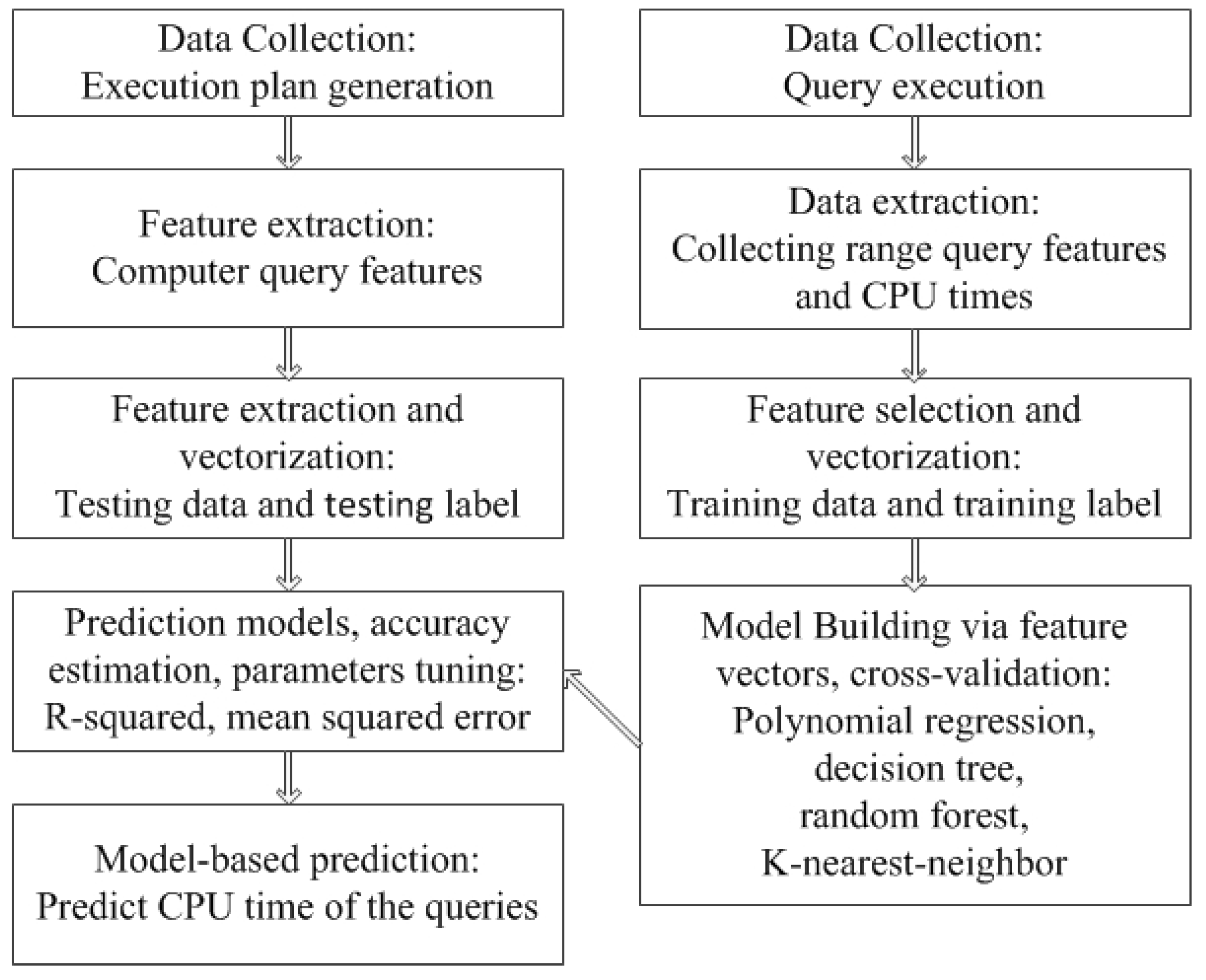
Motivated by that, we propose a method called CPRQ (C ost Prediction of Range Query) to perform CPU time prediction of range queries in MOD. Figure 1 shows the architecture of CPRQ. CPRQ consists of several phases: data collection, feature selection and extraction, feature vectorization, prediction models building, and model-based prediction. Firstly, we design a range query plan generator to collect data. After feature extraction and vectorization of range queries, all prediction models are built and trained to fit the relationship between query features and CPU time. After tuning hyper-parameters of predictive models when training, the learning models are used to predict the CPU time of unforeseen queries in the future. CPRQ utilizes a learning-based method that overcomes the shortcomings generated by the analysis complexity of increasing workload.
In summary, our main contributions are as follows:
- We formalize the problem of predicting range queries over moving objects.
- We propose a method CPRQ to predict the CPU time of range queries. Specifically, we extract features of the queries and encode them using vectors. A prediction model is built.
- We implement the model in an extensible database system SECONDO and conduct experiments using four learning models: polynomial regression, decision tree, random forest, KNN (k-Nearest Neighbor). The experimental results demonstrate the high accuracy of cost prediction for range queries.
The remainder of the paper is organized as follows. We start discussing related work in Section 2. In Section 3, we present the problem definition. We present feature extraction, vectorization and prediction model building of CPRQ in Section 4. The experimental evaluation based on the four learning models’ prediction is provided in Section 5. We discuss our work in Section 6. We conclude the paper in Section 7.
2. Related Work
Cost prediction is a hot topic in the field of database management systems. There has been considerable related work on predicting query cost [22,23,24,25]. These studies are mainly classified into two classic categories: analytical methods and learning methods. There are a variety of metrics for cost prediction that are applicable to analytical methods and/or learning methods. Next, we firstly introduce common metrics for cost prediction, then demonstrate related research studies of analytical methods and learning methods, separately.
In database management systems, different metrics are used to evaluate query cost in various facets. For example, researchers can obtain query cost estimation by modeling the amount of memory [26] and disk space consumed [27] on a target database management system. CPU time is widely used as a cost metric [28,29], which provides a query feedback to users that is more intuitive, compared to other metrics. To effectively support non-traditional data (e.g., moving objects), various index structures are proposed in MODs. Therefore, there are many cost metrics based on the index structure [30], such as the number of disk accesses [11,31] and the selectivity of index nodes [32].
Analytical methods have been the common technique to carry out cost prediction in database management systems [33,34]. The method takes advantage of available expertise on database management systems and encodes the knowledge into mathematical models aimed at capturing how query behaviors map onto query cost [35]. Sun et al. propose an end-to-end learning-based cost estimator for cost estimation [36]. The estimator encodes metadata, query operation, and query predicate into a model. Theodoridis et al. focus on the derivation of analytical formulae based on R-tree to estimate the cost (in terms of node and disk accesses) of selection and join queries in spatial databases [19]. Some analytical methods resort to the optimizer to help analyze the query cost [20]. For example, Markl et al. present a learning optimizer LEO for cost estimation [28], which uses a feedback loop of query statistics.
Analytical methods typically rely on simplified assumptions on how queries execute. Therefore, the accuracy may be seriously challenged in real scenarios in which such assumptions are not matched.
Learning methods lie on the opposite side of the spectrum, given that they require a little knowledge about the target database management systems’ internal behavior. Learning methods treat the database management system as a black-box and rely on the actual behavior to infer a statistical behavioral model [35]. With the rise of machine learning technology, more and more scholars apply learning technologies for cost prediction [22,37]. There are two main reasons for this trend. On the one hand, the ever-increasing complexity of modern database management systems represents the ever-increasing workload for analytical methods’ cost model building. On the other side, analytical methods based on experience and professional knowledge can no longer satisfy the accuracy requirements.
There have been many studies on cost prediction based on machine-learning methods [38,39]. Learning methods are widely used, including logistic regression models [40], random forest models [37], etc. Akdere et al. use a support vector machine to build a separate prediction model for each physical operator and then combine their prediction results to evaluate the query time [41]. Gupta et al. use a binary classification tree to predict the time range of query execution delay. They take the query interaction and concurrency into account [42]. In addition to using a single model to learn query behavior, some researchers attempt to evaluate multiple machine-learning methods. For example, Malakar et al. evaluate 11 machine-learning methods to model the query behavior [43].
Learning methods are promising for the problem of cost prediction. However, the accuracy that they can reach strongly relies on the representativeness of the data set used during the initial training phase.
3. Preliminary
We formalize the range query in MODs and introduce the index structure SETI used for speeding up the query execution.
3.1. Range Query
Definition 1 (Range query).
Given a set of moving objects , a rectangle query window R, a time interval , a range query returns such that , intersects R at t.
We use an example to illustrate the range queries.
Example 1.
The data management system of a certain logistics company stores the information of multiple express cars, including location information and time information of each car every day. A car dispatcher wants to retrieve the information of express cars within fifty miles of the local area for logistics dispatch. Let be the information of multiple express cars, O the information of one car, and t the time stamp of a car within arrival time to departure time. R represents a spatial query window, consisting of a circle with a radius of 50 miles from the dispatcher. The dispatcher designates the time interval . The range query can be written as follows: return the information O for each car from the information sets of multiple express cars, where the O satisfies that there exists a time stamp such that O intersects or overlaps with R at the time stamp t.
3.2. SETI
We perform the cost prediction of range queries based on an index structure called SETI (Scalable and Efficient Trajectory Index) [44]. We designate CPU time as the execution cost because the logical execution cost is intuitive to query effects compared with a physical measure for user experience. SETI makes use of a simple two-level structure to decouple the indexing of the spatial and temporal dimension. The mechanism makes data retrieval very efficient not only for spatial indexing, but also for temporal indexing. Furthermore, SETI has the advantage of being a logical indexing structure that can be easily built over common spatial indexing structures, such as R-tree.
Specifically, SETI partitions spatial objects into a number of non-overlapping spatial cells. A cell contains trajectory segments that are completely within the cell. Each trajectory segment is stored as a tuple in a data file, and a data page only maintains trajectory segments that belong to the same spatial cell. The minimum time interval of each data page represents the time spans of all trajectory segments stored in the page. The time spans of all pages are indexed using an index structure, such as R-tree. These temporal indices are sparse indices because only one entry for each data page is contained instead of one entry for each segment. Moving objects are typically stored in chronological order. The property makes SETI outperform other index structures when retrieving moving objects that overlap with a time range specified in a query.
A range query is formed by a three-dimensional query box, including a temporal predicate box and a time-predicate range. Therefore, there are two steps to perform range queries employing SETI: spatial filtering and temporal filtering. Spatial filtering is applied to pick candidate spatial partitions that overlap with the spatial predicate box. Temporal filtering is employed to extract data pages whose lifetime overlaps with the time predication.
4. CPRQ
CPRQ is an experiment-driven learning technique, which consists of two main phases: training and testing. In the training phase, prediction models are obtained from the training data set, which is represented as a set of feature vectors. In the testing phase, the prediction models are used to predict the CPU time of range queries.
In this section, we firstly analyze the range query features, then encode the features into vectors. Secondly, we introduce the modeling method.
4.1. Feature Extraction and Encoding
We first extract the features of query plans and then encode the features into vectors. Four main factors affect the query cost, including physical query operation, spatial query predicate, temporal query predicate, and data. These features are general features of range queries and are applicable to feature extraction of almost all range queries in different moving object database management systems.
Operation: Operations are physical operators employed in query plans, and different operations can significantly affect the query cost. We consider the and operators based on the SETI index structure. returns all trajectory segments that intersect with the search window, and returns all trajectory segments within the search window. Each operation can be coded as a unique one-hot vector.
One-hot encoding [45], also known as one-bit effective encoding, uses N-bit registers to encode N different values of the features. Each value has an independent register bit, and only one register bit is valid at any time. Specifically, if the feature value has m discrete feature values, the feature after the one-hot encoding operation is an m-dimensional vector, and the feature of each sample can only have one value, that is, the vector coordinate of the value is 1 and the others are 0.
Predicate: A predicate is a filter in a query. Predicates affect query costs because the number of tuples to be retrieved changes when different predicates are applied. A range query is performed only once, but the CPU time of a query is derived from the total execution time, including the spatial filtering time and the temporal filtering time. SETI utilizes a two-layer index structure to separate temporal and spatial dimensions, so we divide predicates into two parts: spatial and temporal predicates. For a query plan, a spatial predicate is a numeric value and we encode it by using normalized floating-point numbers. For the time predicate, we first divide the whole time interval of the data set to be retrieved into different time periods, and the number of data items in each segment is almost the same. Then, we use the one-hot vector to identify the time interval where the temporal condition is located.
Data: Data are a collection of data sets of moving objects. In general, for the same query operation and predicate, the larger the data set, the more computational overhead and query time are incurred. We use n-bit one-hot coding to represent n data sets, each of which corresponds to a 1 significant bit, and the rest of the bits are 0.
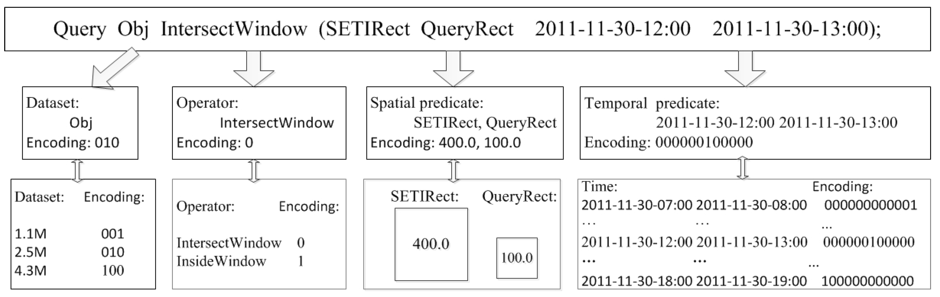
Figure 2 shows an example of feature extraction and encoding. The query plan is “query Obj IntersectWindow (SETIRect QueryRect 2011-11-30-12:00 2011-11-30-13:00)”, where the moving object set contains 2.5 million data points, the operator is , the window size of SETI is 400.0 and the spatial query window size is 100.0. The query plan returns every object within the moving object set indexed by SETI , where the object satisfies intersects with the spatial rectangular query window and the time interval from 2011-11-30-12:00 to 2011-11-30-13:00. We use the one-hot encoding to encode the data set and the predicate. Specifically, the data set in the example contains three sub data sets: 1.1 million data points (1.1 M), 2.5 million data points (2.5 M) and 4.5 million data points (4.5 M). Then, we can encode the 2.5 M we use in the example as 010. For operator and , we use one bit 0 and 1 to encode. For the temporal predicate, we first divide the time span on the data set to be retrieved into time periods, and the number of data items in each time period is the same. Then, we make use of the one-hot encoding to encode the temporal predicate that falls within a certain time period. Specifically, if the time span of is 2011-11-30-07:00 2011-11-30-19:00 and the step to ensure the same number of data items is one hour, then we encode 2011-11-30-07:00 to 000000000001 and 2011-11-30-19:00 to 100000000000. Therefore, the coding of the time period 2011-11-30-12:00 2011-11-30-13:00 to be retrieved in the query plan is 000000100000.
We use a moving object database based on algebraic modules to run queries and collect the data, so we build the feature vector of the algebraic modules. We design a query plan generator to generate query templates. The query plan generator simulates objects moving in a two-dimensional space with query features, and each template contains multiple placeholders. A feature corresponds to a placeholder in a template. The placeholders can be replaced with a specific value. A range query refers to a query in which different placeholders are instantiated.
4.2. Modeling
In this paper, we make a cost prediction in which the cost metric CPU time is a real number; namely, we consider a regression problem. We now turn to the consideration of which type of regression model to train from the collected samples. Machine-learning technologies provide many candidate model types, such as the random forest regression model, some of which were utilized in previous works on predicting query cost. Our selection of the models is driven by two key factors between our problem scenario and previous ones. Firstly, the model can balance errors for unbalanced data sets. Secondly, the model can maintain accuracy when the number of features and samples is not very large. Simple types of instance-based learning model are polynomial regression, decision tree, random forest, and KNN with Euclidean distance. Next, we give the details of the four models.
Polynomial regression: A simple starting point is linear regression. Linear regression means that the relationship between the dependent variables and independent variables is linear. However, there is often more than one independent variable that affects the dependent variable. The study between a dependent variable and one or more independent variables is called polynomial regression. We perform the CPU time prediction for the range query, that is, the predicted variable is only one, so the dependent variable is CPU time and the independent variable includes multiple query features (operation, predicate, and data). Considering that CPU time is affected by multiple query features, we make use of the polynomial regression model.
Decision tree: The decision tree regression model builds a predictive model in the form of a tree structure. The model is composed of multiple judgment nodes. Every node has two or more branches representing values for the attribute tested. Each internal node contains a test using if–else rules to determine which branch the node follows. A leaf node represents a decision on the numerical target. The topmost node in a decision tree is the root node that corresponds to the best predictor. The paper predicts the CPU time of the query execution. We build the decision tree regression model by using the sklearn package of the Python DecisionTreeRegression model.
Random Forest: Important improvements in model accuracy have originated from growing an ensemble of trees by asking them to vote for the predicted value in the random forest regression model. A random forest combines various weak regression trees by taking different samples of the original data set and then combining their outputs. Therefore, the random forest predictive regression model is a meta-estimator that fits some regression trees to each sub-sample of the dataset. Furthermore, the random forest model utilizes the average value to improve the prediction accuracy and control over-fitting. The random forest regression model, RandomForestRegressor, that we used is built by Python’s sklearn package. The model starts with default values.
KNN: KNN is k-Nearest Neighbors, which means that each sample can be represented by its k-Nearest Neighbors. KNN predicts the CPU time based on the k-Nearest Neighbors of the range query instance. We consider the Euclidean distance over the feature space to determine CPU time. The KNN model building consists of two steps. The first step is to find the k points nearest to the node to be predicted. The second step is to take the average value of the k nodes as the predicted value of the point to be predicted. We build the prediction model by using Python’s KNN regressor KNeighborsRegressor with default values. After adjusting the hyperparameters of the model, the KNN regression model is used to predict CPU time.
5. Experimental Evaluation
5.1. Setup
The evaluation is performed in an extensible database system SECONDO [46], which supports range queries over moving objects. SECONDO is scalable by algebra modules and has a friendly user interface. Users can develop data structures and data models and integrate them into SECONDO.
We carry on experiments on a 64-bit Ubuntu Server 14.04 running Intel Xeon(R) 1.90 GHZ CPU, 31 GB system RAM, and a Linux 4.4.0-31-generic operating system. All range queries are executed in SECONDO with a single user model, and the cache size is set as 512 MB.
5.2. Data Sets and Workload
The experimental data sets are real taxi trajectories in Beijing extracted from [47]. Table 1 shows the data statistics. The data sets contain GPS records of 10,357 taxis from 2 February to 8 February 2008, in Beijing. The total number of GPS records is about 15 million and the total distance of trajectories reaches 9 million kilometers. Table 2 exhibits a specific example of the data sets.
We utilize the above query plan generator to generate query testing cases. A query plan is a template with one specific subset, one specific query predicate, and one specific datum that is instantiated with certain values to generate query instances. We use three data sets to collect training and testing data, including 1.1 million, 2.5 million, and 4.5 million data points. To speed up the query execution, we use an index structure SETI. We implement SETI based on R-tree in the experiments. We execute each query plan three times and record the average CPU time in seconds. These queries return at least one result and run within an hour.
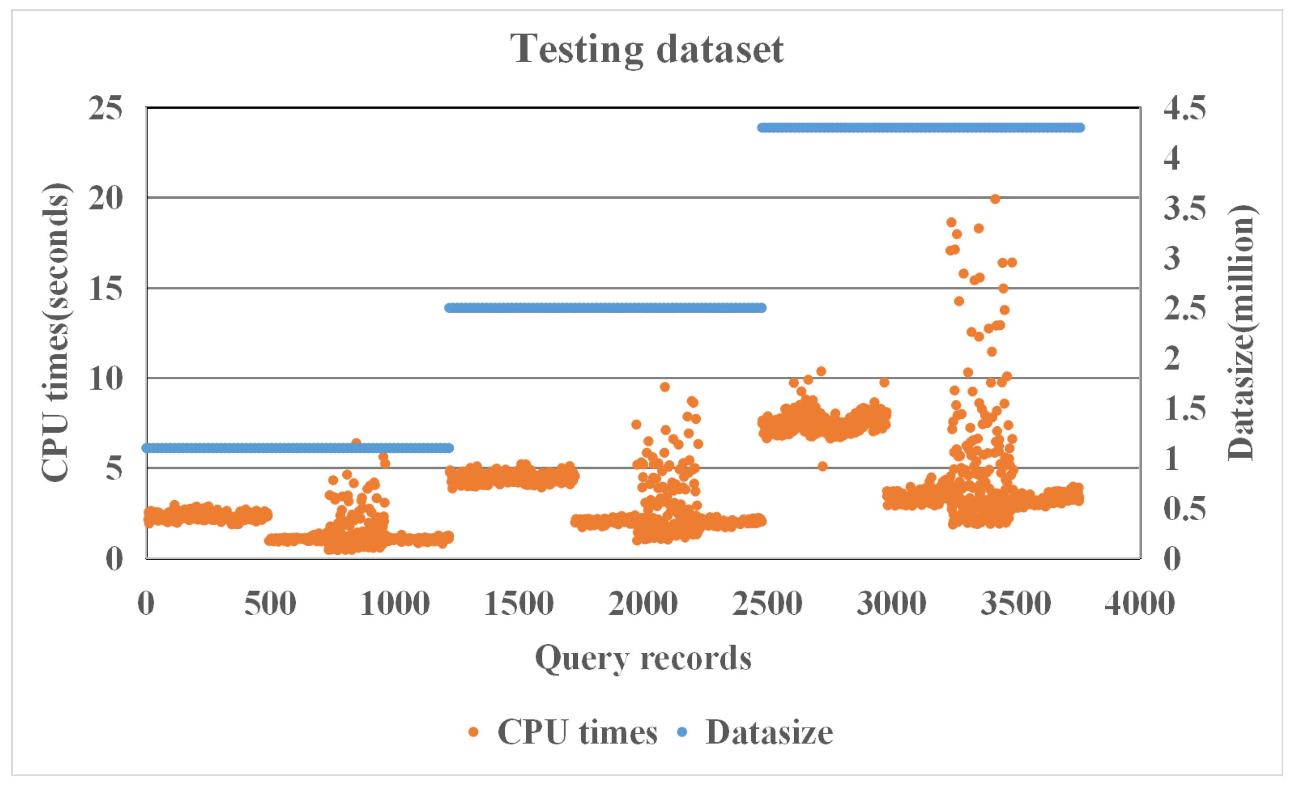
Table 3 shows the details of the training and testing data. There are approximately 4117 queries from each data set. We totally obtain 12,350 records and the average CPU time is 3.3405 s. Figure 3 shows the CPU time distribution of the 12,350 records. We divide the collected data into two disjoint subsets: 70% for training data, that is, 8771 records; and 30% for testing data, that is, 3759 records. We use k-fold cross-validation on the training set, where k is set to 5. The average CPU time of the training data is 3.3209 s. Figure 4 shows the CPU time distribution of the training data set. The average CPU time of the testing data is 3.3622 s. Figure 5 shows the CPU time distribution of the testing data set. We use the query plan template to generate query instances; therefore, these clusters that appear in Figure 3, Figure 4 and Figure 5 indicate that the query features are similar. For example, only varying the spatial predicate in query templates, these queries have similar query characteristics.
5.3. Metrics and Validation
We utilize the R-squared and MSE (Mean Squared Error) as the error metric for measuring the accuracy of the learning models. R-squared is a widely used evaluation metric to evaluate predictive models, which closes to 1, indicating near-perfect prediction. For MSE, the smaller the MSE, the better the prediction accuracy. R-squared and MSE are calculated using the following equation, where is the ground truth objective value for the ith sample in the data set, is the mean of , and denotes the respective predicted value for according sample.
5.4. Performance of Learning Models
We evaluate the prediction accuracy of the four regression models: polynomial regression (PM), decision tree (DT), random forest (RF), and KNN. When training these four models, we tune hyperparameters to obtain each model with the highest accuracy, and then compare the prediction accuracy of the four models in the testing data set.
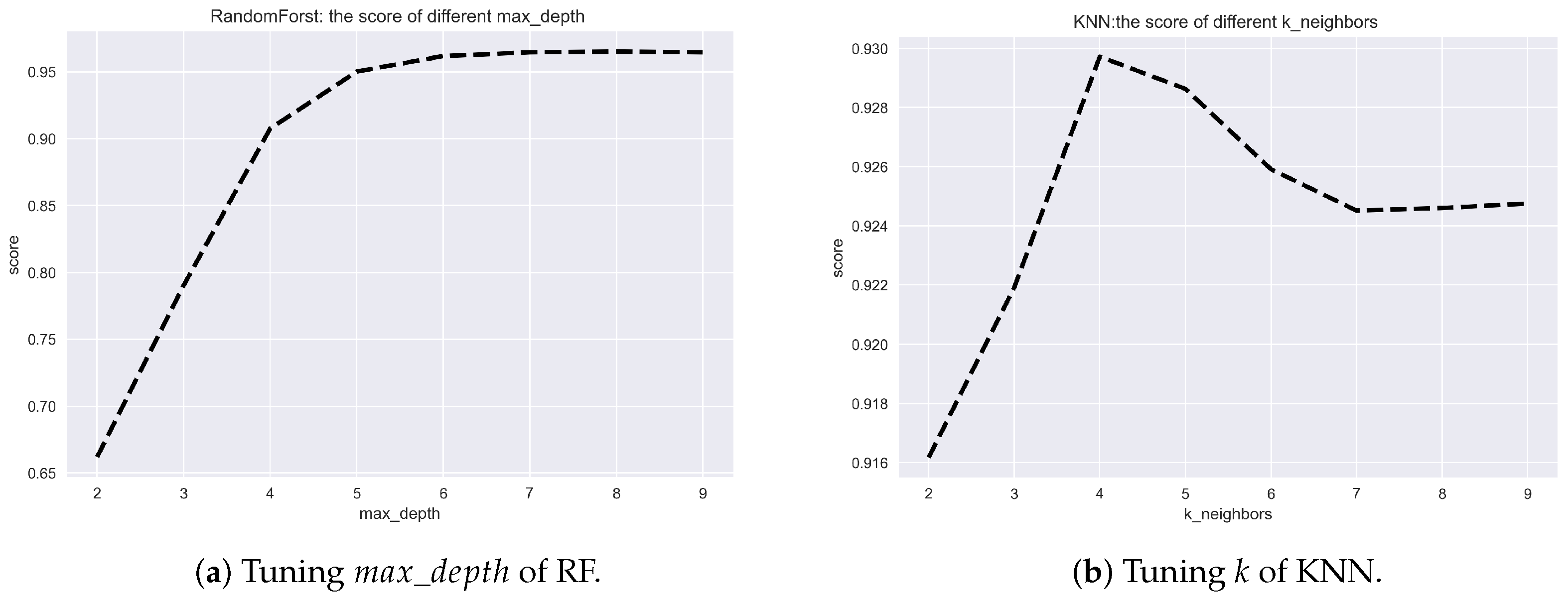
Table 4 shows the hyper-parameters we tune when training the regression model: PM, DT, RF and KNN. For the PM regression model, is used to specify the order of the polynomial used in the resulting polynomial regression. We obtain the best score when is 3. For the DT and RF regression models, determines the maximum depth of the decision tree. The best score is obtained when gets 9 and 9 in the DT and RF regression models, respectively. We tune the hyperparameter k for the KNN regression model and set k to 4. Figure 6 shows the hyper-parameters tuning of RF and k in the RF and KNN regression models.
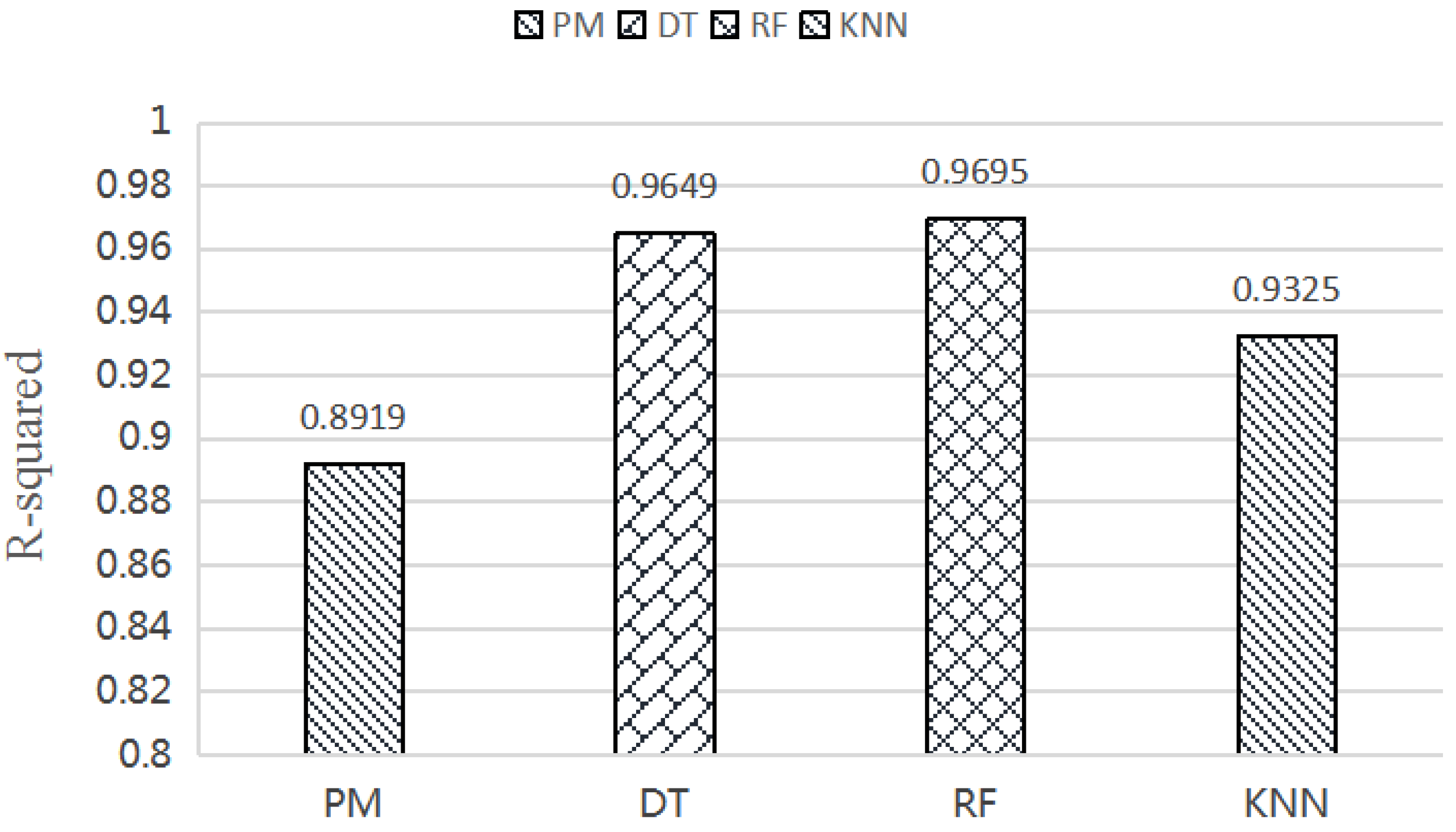
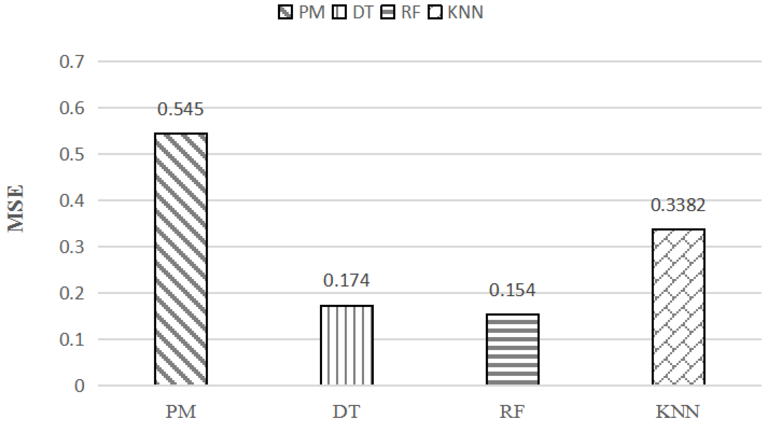
The experimental comparison results of the four models are shown in Figure 7 and Figure 8. In Figure 7 and Figure 8, we find that the R-squared values are all more than 0.8 and the MSE values are all less than 1 of the models. The experimental results show that there is a correlation between the CPU time and the query behavior of the range query. What is more, the machine-learning models with CPRQ can find the correlation and perform the prediction for cost estimation very well.
Specifically, the PM model obtains the minimum value of the R-squared value (0.8919) and the maximum value of MSE (0.545), which implies the relatively poor prediction result compared to the other three models. R-squared and MSE values of the DT and RF model perform in almost the same way with values equal to 0.9649, 0.174, and 0.9695, 0.154. The maximum R-squared value and minimum MSE value indicate that the RF model performs with the best prediction accuracy.
6. Discussion
We propose a technology, CPRQ, to predict the range queries cost in the moving object database management system by modeling the query behavior and CPU time, and evaluate experimentally the four regression models with CPRQ. For future work, we want to address some of the shortcomings that exist in our research. One of the major limitations of CPRQ is that the model predicts the CPU time for range queries while there are many types of queries in the moving object database management. We study the technology to expand the adaptability of the model by integrating different query types to predict the query cost under different query operations. Another disadvantage is that CPRQ is a method based on off-line training progress. Off-line models can accurately predict query costs, but any new data type predictions must retrain the model. We have a work-in-progress to learn the execution cost of query operations in real-time, which can dynamically improve the predictive accuracy of the model. Therefore, this issue will be resolved in the near future.
7. Conclusions
Predicting query costs helps database administrators effectively perform optimal resource schedule strategies. This paper proposes a technology CPRQ, which predicts the query cost of range queries in the moving object database management system by modeling the query behavior and CPU time. CPRQ firstly extracts query features, encodes the features into vectors, and then builds learning models to fit the vectors. We designed a feature extraction method for range queries and evaluated experimentally the four regression models with CPRQ: polynomial regression model, decision tree regression model, random forest regression model, and KNN regression model.
We used R-squared and MSE to evaluate the prediction accuracy of the model. The R-squared and MSE of the polynomial regression model, decision tree regression model, random forest regression model, and KNN regression model were 0.8919 and 0.545, 0.9649 and 0.174, 0.9695 and 0.154, 0.9325 and 0.3382, respectively. The random forest regression model obtained the highest prediction accuracy. The R-squared values of the four models were above 0.89 and MSE values were all within 0.6. The experimental results indicate that CPRQ can accurately predict the CPU time of range queries.
Author Contributions
Conceptualization, Shengnan Guo and Jianqiu Xu; data curation, Shengnan Guo and Jianqiu Xu; formal analysis, Shengnan Guo and Jianqiu Xu; funding acquisition, Jianqiu Xu; investigation, Shengnan Guo; methodology, Shengnan Guo and Jianqiu Xu; project administration, Shengnan Guo and Jianqiu Xu; resources, Jianqiu Xu; software, Jianqiu Xu; supervision, Shengnan Guo and Jianqiu Xu; validation, Shengnan Guo; visualization, Shengnan Guo; writing—original draft, Shengnan Guo; writing—review and editing, Shengnan Guo. Both authors have read and agreed to the published version of the manuscript.
Funding
This work was supported by the National Natural Science Foundation of China (61972198), National Science and Technology Major Project (J2019-II-0014-0035), and Natural Science Foundation of Jiangsu Province of China (BK20191273).
Data Availability Statement
The data presented in this study are available on request from the corresponding author. The data are not publicly available due to restrictions of privacy and morality.
Acknowledgments
The authors thank all the reviewers for the work.
Conflicts of Interest
The authors declare no conflict of interest.
References
- Güting, R.H.; Schneider, M. Moving Objects Databases; Elsevier: Amsterdam, The Netherlands, 2005. [Google Scholar]
- Ding, Z.; Yang, B.; Güting, R.H.; Li, Y. Network-matched trajectory-based moving-object database: Models and applications. IEEE Trans. Intell. Transp. Syst. 2015, 16, 1918–1928. [Google Scholar] [CrossRef]
- Ding, Z.; Guting, R.H. Managing moving objects on dynamic transportation networks. In Proceedings of the 16th International Conference on Scientific and Statistical Database Management, Santorini Island, Greece, 21–23 June 2004; pp. 287–296. [Google Scholar]
- Kohan, M.; Ale, J.M. Discovering traffic congestion through traffic flow patterns generated by moving object trajectories. Comput. Environ. Urban Syst. 2020, 80, 101426. [Google Scholar] [CrossRef]
- Wang, H.; Zimmermann, R. Processing of continuous location-based range queries on moving objects in road networks. IEEE Trans. Knowl. Data Eng. 2010, 23, 1065–1078. [Google Scholar] [CrossRef]
- Iwerks, G.S.; Samet, H.; Smith, K. Continuous k-nearest neighbor queries for continuously moving points with updates. In Proceedings of the 2003 VLDB Conference, Berlin, Germany, 9–12 September 2003; pp. 512–523. [Google Scholar]
- Kaoudi, Z.; Quiané-Ruiz, J.A.; Contreras-Rojas, B.; Pardo-Meza, R.; Troudi, A.; Chawla, S. ML-based cross-platform query optimization. In Proceedings of the 2020 IEEE 36th International Conference on Data Engineering (ICDE), Dallas, TX, USA, 20–24 April 2020; pp. 1489–1500. [Google Scholar]
- Burdakov, A.V.; Proletarskaya, V.; Ploutenko, A.D.; Ermakov, O.; Grigorev, U.A. Predicting SQL Query Execution Time with a Cost Model for Spark Platform. IoTBDS 2020, 279–287. [Google Scholar] [CrossRef]
- Siddiqui, T.; Jindal, A.; Qiao, S.; Patel, H.; Le, W. Cost models for big data query processing: Learning, retrofitting, and our findings. In Proceedings of the 2020 ACM SIGMOD International Conference on Management of Data, Portland, OR, USA, 14–19 June 2020; pp. 99–113. [Google Scholar]
- Negi, P.; Marcus, R.; Mao, H.; Tatbul, N.; Kraska, T.; Alizadeh, M. Cost-guided cardinality estimation: Focus where it matters. In Proceedings of the 2020 IEEE 36th International Conference on Data Engineering Workshops (ICDEW), Dallas, TX, USA, 20–24 April 2020; pp. 154–157. [Google Scholar]
- Papadopoulos, A.; Manolopoulos, Y. Performance of nearest neighbor queries in R-trees. In International Conference on Database Theory; Springer: Berlin/Heidelberg, Germany, 1997; pp. 394–408. [Google Scholar]
- Mohammed, S.; Harris, E.P.; Ramamohanarao, K. Efficient range query retrieval for non-uniform data distributions. In Proceedings of the 11th Australasian Database Conference, ADC 2000 (Cat. No. PR00528), Canberra, Australia, 31 Juanuary–3 February 2000; pp. 90–98. [Google Scholar]
- McCarthy, M.; He, Z.; Wang, X.S. Evaluation of range queries with predicates on moving objects. IEEE Trans. Knowl. Data Eng. 2013, 26, 1144–1157. [Google Scholar] [CrossRef]
- Gorawski, M.; Bugdol, M. Cost Model for X-BR-tree. In New Trends in Data Warehousing and Data Analysis; Springer: Berlin/Heidelberg, Germany, 2009; pp. 1–14. [Google Scholar]
- Ji, X.; Mi, H.; Yang, F.; Shao, Z.; Pan, J. Cost evaluation and improvement of TB-tree insertion algorithm. J. Comput. Methods Sci. Eng. 2018, 18, 445–458. [Google Scholar] [CrossRef]
- Guttman, A. R-trees: A dynamic index structure for spatial searching. In Proceedings of the 1984 ACM SIGMOD International Conference on Management of Data, Boston, MA, USA, 18–21 June 1984; pp. 47–57. [Google Scholar]
- Sellis, T.; Roussopoulos, N.; Faloutsos, C. The R+-Tree: A Dynamic Index for Multi-Dimensional Objects. In Proceedings of the 13th International Conference on Very Large Data Bases, San Francisco, CA, USA, 1–4 September 1987. [Google Scholar]
- Beckmann, N.; Kriegel, H.P.; Schneider, R.; Seeger, B. The R*-tree: An efficient and robust access method for points and rectangles. In Proceedings of the 1990 ACM SIGMOD International Conference on Management of Data, Atlantic City, NJ, USA, 23–25 May 1990; pp. 322–331. [Google Scholar]
- Theodoridis, Y.; Stefanakis, E.; Sellis, T. Efficient cost models for spatial queries using R-trees. IEEE Trans. Knowl. Data Eng. 2000, 12, 19–32. [Google Scholar] [CrossRef]
- Lan, H.; Bao, Z.; Peng, Y. A Survey on Advancing the DBMS Query Optimizer: Cardinality Estimation, Cost Model, and Plan Enumeration. Data Sci. Eng. 2021, 6, 86–101. [Google Scholar] [CrossRef]
- Jitkajornwanich, K.; Pant, N.; Fouladgar, M.; Elmasri, R. A survey on spatial, temporal, and spatio-temporal database research and an original example of relevant applications using SQL ecosystem and deep learning. J. Inf. Telecommun. 2020, 4, 524–559. [Google Scholar] [CrossRef]
- Basu, D.; Lin, Q.; Chen, W.; Vo, H.T.; Yuan, Z.; Senellart, P.; Bressan, S. Regularized cost-model oblivious database tuning with reinforcement learning. In Transactions on Large-Scale Data-and Knowledge-Centered Systems; Springer: Berlin/Heidelberg, Germany, 2016; Volume 28, pp. 96–132. [Google Scholar]
- Chaudhuri, S.; Narasayya, V.R. An Efficient, Cost-Driven Index Selection Tool for Microsoft SQL Server; VLDB: Athens, Greece, 1997; pp. 146–155. [Google Scholar]
- Ahmad, M.; Duan, S.; Aboulnaga, A.; Babu, S. Predicting completion times of batch query workloads using interaction-aware models and simulation. In Proceedings of the 14th International Conference on Extending Database Technology, Uppsala, Sweden, 21–24 March 2011; pp. 449–460. [Google Scholar]
- Ahn, S.; Han, S.; Al-Hussein, M. Improvement of transportation cost estimation for prefabricated construction using geo-fence-based large-scale GPS data feature extraction and support vector regression. Adv. Eng. Inform. 2020, 43, 101012. [Google Scholar] [CrossRef]
- Ganapathi, A.; Kuno, H.; Dayal, U.; Wiener, J.L.; Fox, A.; Jordan, M.; Patterson, D. Predicting multiple metrics for queries: Better decisions enabled by machine learning. In Proceedings of the IEEE 25th International Conference on Data Engineering, ICDE’09, Shanghai, China, 29 March–2 April 2009; IEEE: Piscataway, NJ, USA, 2009; pp. 592–603. [Google Scholar]
- Theodoridis, Y.; Stefanakis, E.; Sellis, T. Cost models for join queries in spatial databases. In Proceedings of the 14th International Conference on Data Engineering, Orlando, FL, USA, 23–27 February 1998; pp. 476–483. [Google Scholar]
- Markl, V.; Lohman, G.M.; Raman, V. LEO: An autonomic query optimizer for DB2. IBM Syst. J. 2003, 42, 98–106. [Google Scholar] [CrossRef]
- Ahmad, M.; Duan, S.; Aboulnaga, A.; Babu, S. Interaction-aware prediction of business intelligence workload completion times. In Proceedings of the 2010 IEEE 26th International Conference on Data Engineering (ICDE 2010), Long Beach, CA, USA, 1–6 March 2010; pp. 413–416. [Google Scholar]
- Lu, Y.; Lu, J.; Cong, G.; Wu, W.; Shahabi, C. Efficient algorithms and cost models for reverse spatial-keyword k-nearest neighbor search. ACM Trans. Database Syst. (TODS) 2014, 39, 1–46. [Google Scholar] [CrossRef] [Green Version]
- Böhm, C. A cost model for query processing in high dimensional data spaces. ACM Trans. Database Syst. (TODS) 2000, 25, 129–178. [Google Scholar] [CrossRef]
- Jin, J.; An, N.; Sivasubramaniam, A. Analyzing range queries on spatial data. In Proceedings of the 16th International Conference on Data Engineering (Cat. No. 00CB37073), San Diego, CA, USA, 28 February–3 March 2000; pp. 525–534. [Google Scholar]
- Wu, W.; Chi, Y.; Zhu, S.; Tatemura, J.; Hacigümüs, H.; Naughton, J.F. Predicting query execution time: Are optimizer cost models really unusable? In Proceedings of the 2013 IEEE 29th International Conference on Data Engineering (ICDE), Brisbane, Australia, 8–12 April 2013; pp. 1081–1092. [Google Scholar]
- Hendawi, A.M.; Mokbel, M.F. Panda: A predictive spatio-temporal query processor. In Proceedings of the 20th International Conference on Advances in Geographic Information Systems, Redondo Beach, CA, USA, 6–9 November 2012; pp. 13–22. [Google Scholar]
- Didona, D.; Quaglia, F.; Romano, P.; Torre, E. Enhancing performance prediction robustness by combining analytical modeling and machine learning. In Proceedings of the 6th ACM/SPEC International Conference on Performance Engineering, Austin, TX, USA, 28 January–4 February 2015; pp. 145–156. [Google Scholar]
- Sun, J.; Li, G. An end-to-end learning-based cost estimator. arXiv 2019, arXiv:1906.02560. [Google Scholar]
- Quoc, H.N.M.; Serrano, M.; Breslin, J.G.; Phuoc, D.L. A learning approach for query planning on spatio-temporal IoT data. In Proceedings of the 8th International Conference on the Internet of Things, Santa Barbara, CA, USA, 15–18 October 2018; pp. 1–8. [Google Scholar]
- Hasan, R.; Gandon, F. A machine learning approach to sparql query performance prediction. In Proceedings of the 2014 IEEE/WIC/ACM International Joint Conferences on Web Intelligence (WI) and Intelligent Agent Technologies (IAT), Warsaw, Poland, 11–14 August 2014; pp. 266–273. [Google Scholar]
- Wan, S.; Zhao, Y.; Wang, T.; Gu, Z.; Abbasi, Q.H.; Choo, K.K.R. Multi-dimensional data indexing and range query processing via Voronoi diagram for internet of things. Future Gener. Comput. Syst. 2019, 91, 382–391. [Google Scholar] [CrossRef] [Green Version]
- Duggan, J.; Cetintemel, U.; Papaemmanouil, O.; Upfal, E. Performance prediction for concurrent database workloads. In Proceedings of the 2011 ACM SIGMOD International Conference on Management of Data, Athens, Greece, 12–16 June 2011; pp. 337–348. [Google Scholar]
- Akdere, M.; Cetintemel, U.; Riondato, M.; Upfal, E.; Zdonik, S.B. Learning-based query performance modeling and prediction. In Proceedings of the 2012 IEEE 28th International Conference on Data Engineering, Washington, DC, USA, 1–5 April 2012; pp. 390–401. [Google Scholar]
- Gupta, C.; Mehta, A.; Dayal, U. PQR: Predicting query execution times for autonomous workload management. In Proceedings of the 2008 International Conference on Autonomic Computing, Chicago, IL, USA, 2–6 June 2008; pp. 13–22. [Google Scholar]
- Malakar, P.; Balaprakash, P.; Vishwanath, V.; Morozov, V.; Kumaran, K. Benchmarking machine learning methods for performance modeling of scientific applications. In Proceedings of the 2018 IEEE/ACM Performance Modeling, Benchmarking and Simulation of High Performance Computer Systems (PMBS), Dallas, TX, USA, 12 November 2018; pp. 33–44. [Google Scholar]
- Chakka, V.P.; Everspaugh, A.; Patel, J.M. Indexing Large Trajectory Data Sets with SETI; CIDR: Asilomar, CA, USA, 2003. [Google Scholar]
- Harris, D.; Harris, S. Digital Design and Computer Architecture; Morgan Kaufmann: Burlington, MA, USA, 2010. [Google Scholar]
- Lu, J.; Güting, R.H. Parallel secondo: A practical system for large-scale processing of moving objects. In Proceedings of the 2014 IEEE 30th International Conference on Data Engineering, Chicago, IL, USA, 31 March–4 April 2014; pp. 1190–1193. [Google Scholar]
- Yuan, J.; Zheng, Y.; Zhang, C.; Xie, W.; Xie, X.; Sun, G.; Huang, Y. T-drive: Driving directions based on taxi trajectories. In Proceedings of the 18th SIGSPATIAL International Conference on Advances in Geographic Information Systems, San Jose, CA, USA, 2–5 November 2010; pp. 99–108. [Google Scholar]
Figure 1.
The architecture of CPRQ.

Figure 2.
Example of feature extraction and encoding.

Figure 3.
The CPU time distribution of training and testing data sets.

Figure 4.
The CPU time distribution of training dataset.

Figure 5.
The CPU time distribution of testing data set.

Figure 6.
Hyper-parameters tuning.

Figure 7.
R-squared values of polynomial regression (PM), decision tree (DT), random forest (RF) and KNN.
Figure 7.
R-squared values of polynomial regression (PM), decision tree (DT), random forest (RF) and KNN.

Figure 8.
MSE values of polynomial regression (PM), decision tree (DT), random forest (RF) and KNN.


Table 1.
Beijing taxi data set.
| Taxi | GPS Records | Longitude | Latitude | Duration |
|---|---|---|---|---|
| 10,357 | 15,000,838 | [115.42, 117.5] | [39.42, 41.05] | [2 February 2008, 8 February 2008] |
Table 2.
A specific example of Beijing taxi data set.
| Trajectory id | Time | Longitude | Latitude |
|---|---|---|---|
| ... | ... | ... | ... |
| 10 | 2 February 2008 13:32:08 | 116.442194 | 39.993146 |
| 10 | 2 February 2008 13:32:13 | 116.442174 | 39.993178 |
| 10 | 2 February 2008 13:32:18 | 116.442166 | 39.993211 |
| ... | ... | ... | ... |
Table 3.
Training and testing data sets.
| Description | Data Set | Training Data Set | Testing Data Set |
|---|---|---|---|
| Number of records | 12,530 | 8771 | 3759 |
| Average execution time (s) | 3.3405 | 3.3209 | 3.3622 |
Table 4.
The hyper-parameters tuning when training PM, DT, RF and KNN.
| Model | ||||
|---|---|---|---|---|
| Hyper-parameter(s) | k | |||
| Range | [1, 10] | [2, 9] | [2, 9] | [2, 9] |
| The value with the best score | 3 | 9 | 9 | 4 |
Publisher’s Note: MDPI stays neutral with regard to jurisdictional claims in published maps and institutional affiliations. |
© 2021 by the authors. Licensee MDPI, Basel, Switzerland. This article is an open access article distributed under the terms and conditions of the Creative Commons Attribution (CC BY) license (https://creativecommons.org/licenses/by/4.0/).
Share and Cite
MDPI and ACS Style
Guo, S.; Xu, J. CPRQ: Cost Prediction for Range Queries in Moving Object Databases. ISPRS Int. J. Geo-Inf. 2021, 10, 468. https://0-doi-org.brum.beds.ac.uk/10.3390/ijgi10070468
AMA Style
Guo S, Xu J. CPRQ: Cost Prediction for Range Queries in Moving Object Databases. ISPRS International Journal of Geo-Information. 2021; 10(7):468. https://0-doi-org.brum.beds.ac.uk/10.3390/ijgi10070468
Chicago/Turabian StyleGuo, Shengnan, and Jianqiu Xu. 2021. "CPRQ: Cost Prediction for Range Queries in Moving Object Databases" ISPRS International Journal of Geo-Information 10, no. 7: 468. https://0-doi-org.brum.beds.ac.uk/10.3390/ijgi10070468
Note that from the first issue of 2016, this journal uses article numbers instead of page numbers. See further details here.