Creation of a Multimodal Urban Transportation Network through Spatial Data Integration from Authoritative and Crowdsourced Data

Abstract

One of the most significant challenges in cities concerns urban mobility. Urban mobility involves the use of different modes of transport, which can be individual or collective, and different organizations can produce their respective datasets that, usually, are used isolated from each other. The lack of an integrated view of the entire multimodal urban transportation network (MUTN) brings difficulties to citizens and urban planning. However, obtaining reliable and up-to-date spatial data is not an easy task. To address this problem, we propose a framework for creating a multimodal urban transportation network by integrating spatial data from heterogeneous sources. The framework standardizes the representation of different datasets through a common conceptual model for spatial data (schema matching), uses topological, geometric, and semantic information to find matches among objects from different datasets (data matching), and consolidated them into a single representation using data fusion techniques in a complementary, redundant and cooperative way. Spatial data integration makes it possible to use reliable data from official sources (possibly outdated and expensive to produce) and crowdsourced data (continuously updated and low cost to use). To evaluate the framework, a MUTN for the Brazilian city of Belo Horizonte was built integrating authoritative and crowdsourced data (OpenStreetMap, Foursquare, Facebook Places, Google Places, and Yelp), and then it was used to compute routes among eighty locations using four transportation possibilities: walk, drive, transit, and drive–walk. The time and distance of each route were compared against their equivalent from Google Maps, and the results point to a great potential for using the framework in urban computing applications that require an integrated view of the entire multimodal urban transportation network.

1. Introduction

People continuously move around the city going to work, school, sports facilities, and other entertainment activities. Planning for urban mobility requires up-to-date spatial and temporal data about individual and collective transportation modes. Individual transportation modes include “any mode where mobility is the outcome of a personal choice and means such as the automobile, walking, cycling, or the motorcycle” [1]. Collective transportation (or public transit) modes involve shared vehicles and a pre-established route, schedule, and a fee. Such modes include tramways, buses, trains, subways and ferryboats.

Urban mobility data are usually produced and maintained by a large number of agencies, applications, and users. Each one has specific needs, and therefore maintains its own policy regarding data dissemination, which can cause a high level of data inconsistency and heterogeneity [2]. The integration of data from several heterogeneous sources on different transportation modes remains a challenge [3,4], which reflects on difficulties for citizens that need to move across the city [5] and hampers the decision making of urban planners by lacking an integrated view of the entire multimodal transportation network.

Another difficulty is in obtaining reliable and up-to-date urban data. There are two primary sources for such data: authoritative or voluntary. Authoritative data are usually produced by governmental agencies at a high production cost, therefore are highly reliable, but difficult to keep up-to-date [6,7]. Voluntarily contributed data uses the population as producers (or sensors), often for free. Reliability is often an issue, but updating frequency can be high and coverage can be extensive if there are enough volunteers. Complementing and updating official source data with volunteered data is increasingly necessary, especially in places with little infrastructure for urban data maintenance [6].

In the case of urban mobility, the availability of such diverse data sources, most of which rooted in daily operational needs and focused in parts of the system, contrasts with the need for an integrated view of mobility. With an integrated view, we become able to analyze mobility as a whole, considering the ongoing processes and their continuous transformation, and plan for their evolution.

In this paper, we propose a framework for integrating spatial data from heterogeneous sources to produce a multimodal urban transportation network dataset that can be used in various urban computing applications. For schema matching, we propose transforming each source schema to a standard spatial conceptual data model. For spatial data matching, we present a method using topological, geometric and semantic information to identify matches among objects from different datasets. Matched objects are then consolidated into a single representation using data fusion techniques, but objects that are unique to a given data source are included whenever necessary, since data sources are mostly complementary, rather than thematically overlapping. We use the framework to build a multimodal urban transportation dataset integrating authoritative and crowdsourced data.

We validate our approach using real-world data to build a multimodal urban transportation network dataset for the city of Belo Horizonte, in Brazil. The result are evaluated by generating multimodal routes among random points and comparing the results with routes provided by Google Maps. The results enable us to analyze, simulate, and compute analytical data considering the whole multimodal transportation urban network instead of isolated views from each mode of transport. The integration of up-to-date voluntarily contributed data with authoritative sources can also be used to identify areas where official data are out of date and to optimize official mapping work in a targeted way.

The remainder of this paper is organized as follows. Section 2 presents concepts and related work. Section 3 describes our multimodal urban transportation network data model. Section 4 details the process to build the multimodal transportation network from multiple sources using data integration techniques. A case study using the proposed approach for Belo Horizonte is described in Section 5. Results are presented and discussed in Section 6. Finally, Section 7 concludes the paper and presents future work directions.

2. Concepts and Related Work

We propose the creation of a multimodal urban transportation network dataset from heterogeneous sources using spatial data integration techniques. Such a dataset can be enriched with data from additional sources. For instance, aspects related to transit user experience can be crowdsourced, and sensor data on traffic dynamics can be included. Our framework includes a conceptual schema for a spatial database, used as a reference for schema matching. Integration of data from various sources is then organized around this conceptual schema, and therefore data might need to be transformed before inclusion in the integrated dataset. Data matching between datasets, when required, is performed considering mainly the geometric similarity among objects, and also topological and semantic aspects. Once matching pairs of objects considered to be equivalent are found, they are consolidated in the integrated dataset (Data Fusion). Objects that have no match in other datasets are also evaluated and transformed for integration.

The resulting dataset, following the proposed conceptual schema, can be used in applications that require an integrated view of urban mobility, both individual and collective. The remainder of this section presents concepts and related work on multimodal urban transportation networks and spatial data integration.

2.1. Multimodal Urban Transportation Networks

A Multimodal Urban Transportation Network (MUTN) is an essential component when dealing with urban analysis. Nes [8] defines a multimodal transport as one in which at least two different modes are used, and the traveler has to make a transfer from one mode to another. Likewise, Mandloi and Thill [9] and Chen et al. [10] characterize multimodal transport whenever the movement of people or goods involves at least two modes of transport from origin to destination. Zuidgeest et al. [11] see MUTN as a set of subsystems, where each one represents a transport mode. The connections among systems are implemented as exchange points at nodes or terminals. People can only change to a different mode using a terminal. However, when multiple modes are available, and modes are managed by different organizations, there is often no integrated view of the entire system.

A MUTN has to manage data about the street network, and also on the entire transport infrastructure (streets, rail, bus stations), and transport services of each mode (car, walking, cycling, bus, metro). It is also desirable to enrich the MUTN with data from non-conventional data sources, including crowdsourcing, to better understand the patterns and interactions of urban life. For example, Zheng and Geroliminis [12] built a multimodal traffic model considering parking constraints using a macroscopic fundamental diagram (MFD) to define parking pricing strategies to reduce congestion and overall travel costs to drivers. The work focused on numerical modeling for the choice of modal to be used, and was performed using a simulated urban transport network considering only cars and buses. Gil [13] used OpenStreetMap (OSM) data to build a MUTN to enable accessibility analysis. OSM data for collective transport was complemented with data from an official source (OpenOV), but in a simplified form, without considering details such as the lines, services, and their frequencies. Jetlund et al. [14] proposed a generic data model for transport data, based on ISO and INSPIRE standards, focused on data interoperability.

The MUTNs resulting from these works were built for specific purposes, while our approach proposes a broader model that can be used for various applications and can incorporate additional data. We also use data from different and heterogeneous sources using data integration methods, which are presented in the next Section.

2.2. Spatial Data Integration

Spatial data plays an essential role in the decision-making process. It is estimated that about 80% of all information used on the decision-making process have spatial properties [15,16], and its correct use implies better decisions [17].

The Open Geospatial Consortium (OGC) defines spatial data integration as “the process of unifying two or more separate datasets, which share certain characteristics, into one integrated all-encompassing result” [18]. The outcome of spatial data integration is not just data overlayed and displayed together. It must have connections among features in different datasets and merge them into a single representation hoping to find new knowledge that cannot be derived from the individual datasets alone [19,20,21,22]. Data sources used in the referenced works concerning spatial data integration can be classified into two categories: official (or authoritative) and volunteered geographic information (VGI). Official data are generally produced by government agencies, while VGI data is produced collaboratively by citizens and contributors. Among the primary VGI services are OpenStreetMap (https://www.openstreetmap.org (accessed on 21 June 2021)) (OSM) and Waze (https://www.waze.com (accessed on 21 June 2021)). The high cost of production to create and maintain official spatial data and the increasing availability of VGI initiatives have encouraged researchers and governments to seek ways to integrate these data sources to obtain a more up-to-date dataset with a lower production cost [6,23,24,25,26,27,28].

Spatial data integration can be organized into three main tasks [29]. The first task is schema matching, which seeks to establish the semantic correspondence between object classes from different datasets [30]. Once the semantics are resolved, the second task, data matching, takes place to identify corresponding dataset objects. The third and last task, called data fusion, involves the resolution of schematic and representation differences among matched objects to produce a single and consistent representation. Some works do not consider schema matching and data matching as independent tasks, and suggest viewing them as components of a more general task within the data integration process [31,32,33,34].

2.2.1. Schema Matching

Schema matching involves finding semantic correspondences between elements from different schemas [30,35]. Schema matching techniques rely on schema information (data types, element names, and structural properties) [36] attributes of object instances, or external information, such as ontologies and dictionaries [2,36,37,38,39].

Since matching schemas is primarily an exercise on modeling semantics, ontologies are frequently used in the literature. Al-Bakri and Fairbairn [36] worked on Ordnance Survey and OpenStreetMap integration at schema level (based on XML) using three metrics: name similarity between classes, structural similarity between schemas and data type similarity. The metrics were combined in a weighted similarity measure to resolve possible matches, but did not obtain excellent results, therefore suggesting the use of more directed ontologies to improve the spatial data integration process. Du [39] used ontologies to integrate authoritative (Ordnance Survey) and crowdsourced (OpenStreetMap) data on roads [40] and other real data. Their method converts the input datasets to ontologies, and then merge them into a new ontology. Guan et al. [37] used ontologies to match Geographic Markup Language (GML) schemas, and tested the proposal over data on highways and roads (among other kinds of data, such as states, cities, rivers, and lakes) from Canada and the USA. Prudhomme et al. [2] applied a semantic interpretation process to infer an ontology from a dataset schema without prior knowledge. The produced ontology is then used for schema matching through the use of ontology matching techniques. Their approach for semantic interpretation is based on geocoding and natural language processing.

For this work, although semantic or ontology-based schema matching would be possible, we decided to perform schema matching manually, by comparing documentation on the schema of each source to the proposed conceptual schema. For the case of transportation data, schema matching is facilitated by the use of similar spatial representations for the most important object classes.

2.2.2. Spatial Data Matching

Spatial data matching can be defined as the correct correspondence between different dataset objects [26] and is a requirement for integration, management, and quality evaluation of spatial datasets [34]. It can also be called linking [40], alignment [41] or reconciliation [42,43].

There are many taxonomies for spatial data matching techniques on literature [34,44,45,46,47,48]. Xavier et al. [34] proposed a broad classification based on two criteria: level and case of correspondence. The level refers to where, in the data modeling hierarchy, the matching will occur. Three alternatives are possible: schema, feature and internal. The schema level is equivalent to the schema matching concepts presented in Section 2.2.1. Feature level matching methods consider that schema matching is already complete, and work to find correspondences among features using one or more similarity measures. Internal level matching regards the comparison of parts of geometric features, which is essential for quality assessment [49,50,51]. The case of correspondence regards the cardinality of the matching, and can be defined as one-to-one (1:1), one-to-many (1:N) and many-to-many (M:N).

Feature matching methods involve looking for candidate features for matching in dataset $\mathcal{B}$ that are close to a feature in dataset $\mathcal{A}$ and then checking the similarity of each candidate feature to characterize a match. Among the common techniques for finding candidate features are the use of buffers [2,28,52,53,54,55] and algorithms for finding nearest neighbors [47,56]. Similarity metrics can be classified into geometric, topological, attribute-based, context-based, and semantic [34].

Geometric metrics use geometric characteristics of features such as position, length, perimeter, area, shape, or angle [57]. Among the most used metrics in this category are Euclidean [20,58,59,60,61,62], Hausdorff [2,45,47,63,64,65,66] and Fréchet [2,67,68] distances, shape similarity measures [2,49,51], and the degree of overlapping between features [2,27,69,70].

Topological metrics analyze the spatial relationships among features and are most used to match network (node-arc) structures. Many graph characterization metrics are used, such as, node degree [71,72], centrality [27,73], betweenness [73,74,75] and closeness [73,75].

Attribute-based metrics are used to compare features based on non-spatial associated data. This category of similarity measures relies on operators for comparing attribute data types. The most commonly used metrics involve string comparisons, such as Levenshtein distance [76,77] and Hamming distance [64].

Context-based metrics use the geographic context of the features to help determine their similarity. Geographic context refers to the relationships between a feature and other reference features. It works by using a list of known points (landmarks) that can be used to build a proximity graph [76], a Delaunay triangulation or a Voronoi diagram [54,60] to compute the similarity between candidate features.

Semantic metrics determine the distance between concepts of the features, where the concepts can be classes, methods or attributes [34]. The difficulty in applying such methods is that some formal representation of knowledge, like an ontology or taxonomic tree, is usually required. Hastings [78] used the least common superconcept (LCS) in a taxonomic tree to evaluate the similarity between gazetteer terms by counting the number of (possibly weighted) steps on the tree necessary to navigate from one concept to another.

Much research on using techniques and methods for spatial data matching can be found in the literature. We focus our attention on those involving the integration between authoritative and crowdsourced data of urban and transportation data.

Mustiere and Devogele [58] proposed NetMatcher, a feature matching process that uses geometrical, attribute-based and topological similarity metrics to find and evaluate potential candidates for matching, even with different levels of details, so it can deal with one-to-many and many-to-many correspondence cases.

Ludwig et al. [79] compare OSM road data with a Navteq dataset. They segment road segments data from OSM to level the number of features on both datasets and then use buffer operations to ease finding one-to-one correspondences. Then, the length, category, and name of features are used as similarity metrics to find the best candidates to match.

Koukoletsos et al. [80] use a multi-stage approach for feature matching, combining geometric (distance, direction, length of roads) and attribute-based (road names, road types) metrics to assess the completeness of OSM data concerning the ordnance survey dataset. They use a 1 km² grid to clip the datasets and then each cell is analyzed to find matchings. Characteristics of VGI data, such as topological inconsistencies and abbreviations used on feature names, may affect the results.

Yang et al. [81] developed a heuristic probabilistic relaxation method to match road networks from OSM and authoritative data at the feature level. The method starts with a probabilistic matrix built from similarity measures on feature shapes and then incorporates compatibility coefficients of neighboring candidates until the probabilistic matrix gets globally consistent. Then, it finds one-to-one matching pairs and then expands to find many-to-many matchings. It also considers null matches (a one-to-null or 1:0 correspondence level) to include data that are unique to one of the sources, possibly in places the other source is outdated or incomplete. The matching results showed high precision using only geometric similarity metrics, but the method is computationally costly.

Fan et al. [24] used a polygon-based approach to match road networks at feature level. The first step matches urban block polygons verifying overlapping areas. Then, road segments are assigned to the edges of the urban blocks. Those road segments assigned to the same edge of a matched urban block pair are considered a match. The results showed high matching rates, but it does not match roads that cannot be assigned to a nearby urban block, or no-through roads that do not form a closed polygon.

Abdolmajidi et al. [66] compared segment-based and node-based approaches for roads matching at feature level. They choose the node-based approach due to the reduced computational cost and improve it to handle topological relationships and other network components. It was used geometric (segment orientation and length), topological (checking the links and neighbors of a node) and attribute-based (feature name) similarity metrics on the matching process. The resulting method is used to assess the completeness of OSM data in relation to the Swedish National Road Database.

Olteanu-Raimond et al. [82] present a data matching approach based on knowledge fusion using belief theory. They model geometrical (position, orientation), semantic, attribute-based (name of the feature), and contextual similarity metrics into belief functions to find correct matching pairs.

In this work, the data matching process occurs at the feature level. For line features the process starts with the creation of a list of candidates for matching by finding features from one dataset that intersects the buffer of a feature in the other dataset. If a feature has no candidate for matching it is considered as (a null match, or one-to-zero). Then, the list is used to find matching pairs with one-to-one, one-to-many (or many-to-one), and many-to-many cardinalities. To confirm a pairing, geometric similarity metrics such as node proximity, length and angle similarity of the segments are used. For point features we also create a list of possible matches using a KD-tree to speed up the search. The matches are confirmed using geometric (distance), semantic (the type of the feature) and attribute-based (name) similarity metrics used. For name similarity it is used the Levenshtein distance; however, we introduce a treatment to reduce problems in name matching. The names are converted to lowercase, tokenized, sorted alphabetically and concatenated. The tokenization drops punctuation characters, and the sorting allows for more precise matching when the names differ only in word order (a common situation for names in crowdsourced data).

2.2.3. Spatial Data Fusion

The result of the spatial data matching task is a set of matched pairs of elements from the datasets being integrated. The next step is to use the matched pairs across the databases to find the underlying true values in case of conflicts [83]. This is the responsibility of spatial data fusion step on spatial data integration process [84,85]. To illustrate the problem faced by spatial data fusion, consider the following situation. Two road objects, ${\mathcal{R}}_a$ and ${\mathcal{R}}_b$ are from different spatial data sets with slightly different geometries and similar values for the name attribute. Which object best represents the geometry of the actual road? Which one has the most accurate version of the name of the road? The desired output is a road object that has the best real-world correspondence for every considered attribute.

The techniques employed in data fusion can be classified in different ways [86], such as by the relationship between the data sources [87]. In this case, the data sources involved in the fusion process can be complementary, redundant, or cooperative. Figure 1 shows an overview of these categories. In complementary data fusion, the input data sources represent different views of the same subject so that one can complement the information present in the other and generate a more complete unified version of the data. In redundant data fusion, the same subject is represented in different data sources that can be unified to increase confidence in this data. In cooperative data fusion, data from the input sources are combined into new information that is usually more complex or more complete than the original sources.

In data fusion, especially of the redundant type, it is necessary to employ conflict resolution strategies to conduct the transfer or fusion of information between the attributes of the paired features. The strategy to be employed depends on the characteristics of the data sources, the available data and the desired output. Bleiholder and Naumann [85] presents a taxonomy for strategies for dealing with data conflicts based on three primary strategies: conflict ignorance, conflict avoidance and conflict resolution.

Our framework performs spatial data fusion tasks at various times. When building the street network, attribute values (road name, functional classification, and width) that are missing in one of the datasets and are present in the other in the paired features are updated, which configures a redundant data fusion. Unique street sections from one dataset, as well as other information (parking lots, public transport), can be included in the fusion result (complementary fusion). In the creation of the multimodal network, the data are organized to allow routing throughout the network and its different modes, which classifies the fusion process as cooperative. The resulting multimodal urban transport network allows analysis and operations based on an integrated view of urban transport that would be difficult or impossible if the datasets were used in isolation. The framework proposes and uses a spatial data model along the data integration process and to store the results. The spatial data model are discussed in the following section.

3. Multimodal Urban Transportation Network Data Model

The Multimodal Urban Transportation Network (MUTN) model represents the integrated infrastructure of urban transport, considering individual and collective transportation modes. The individual mode comprises the infrastructure for private or shared vehicles (including taxis, rentals, car sharing, bicycles, and others) and pedestrians, while the collective transportation mode is responsible for public transit such as bus and metro systems. The difference between them is that the public transit system typically follows a pre-established structure where routes, stops, and schedules are defined. Multiple agencies may be responsible for the management of public transit alternatives. The network for each mode of transport is represented geographically, using geospatial coordinates, and topologically, using directed graphs. The remainder of this section explains the structure and functionality of the data model classes.

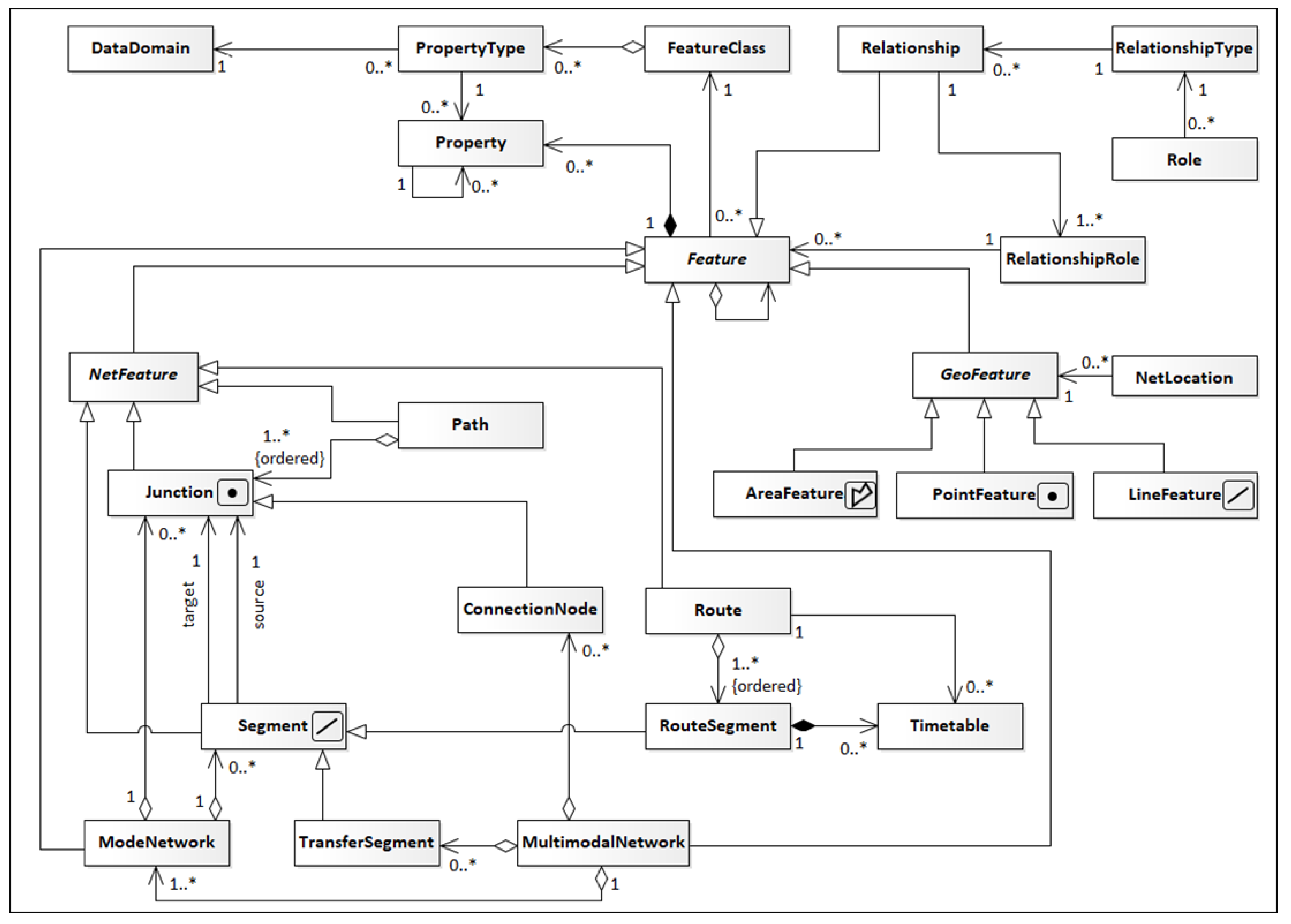
We introduce a conceptual schema (Figure 2) to be used as the basis for data integration, including schema matching, data matching and data fusion. All source datasets must be matched and transformed as needed to fit the proposed schema. Next, we describe the proposed schema in detail.

The Property class stores attributes for each feature using a key-value schema, where the key is an instance of the PropertyType class that has a name and a domain, given through the DataDomain class. In turn, the DataDomain class has a name, a data type, and a unit (e.g., km/h, meters, seconds, and other measurement units) for the interpretation of values associated with the domain.

The main building block of the MUTN model is the abstract Feature class. A feature represents a real-world object or a relationship among features. It must have a unique identification (fid) and belong to a FeatureClass. Features may have a set of properties. The FeatureClass contains all possible feature types the data model can use, and store information about the properties for each feature class. A Feature can be specialized as a Relationship, a GeoFeature, a NetFeature, a ModeNetwork or a MultimodalNetwork.

In many situations in modeling, we need to establish relationships between several features so that each one can play a role in a relationship with others. The Relationship, RelatioshipRole, RelationshipType, and Role classes are used in these situations. RelationshipType and Role define relationships for each one of the possible roles a feature can assume. For example, consider a forbidden conversion constraint between $s_1$ and $s_2$ segments passing through road junction $j_1$. This constraint can be modeled as follows: There must be a ‘no_turn’ RelationshipType associated with ‘from’, ‘via’, and ‘to’ roles, a new instance of the Relationship class with type ‘no_turn’ and three new instances of the RelationshipRole class are created for the segment $s_1$, junction $j_1$, and segment $s_2$ in the roles ‘from’, ‘via’, and ‘to’, respectively.

The abstract class NetFeature represents features that relate to others in topological structures to form networks. A NetFeature can be a Junction, a Segment, a Path, or a Route. A Junction corresponds to a network node, but with a geographic representation. The Path class is used to represent a path through the transportation network using an ordered sequence of Junctions. The Route class is used to represent a collective transportation service with fixed schedule, for example, a bus or subway line. Junction and Segment classes are the basis for establishing network structures as the ModeNetwork class. In the proposed data model, the networks are modeled as directed graphs. From graph theory, a directed graph is defined as an ordered pair $G=(V,E)$, where V is a set of vertices, and E is a set of edges, defined as ordered pairs of vertices. In the MUTN data model, a ModeNetwork represents the network for one mode of transport as a directed graph in which the vertices and edges are Junctions and Segments, respectively.

Every Segment starts and ends at a Junction whose identifiers are stored in the segment as its ‘source’ and ‘target’ attributes. The direction of the flow through the segment is always from source to target. There are other mandatory attributes for segments besides source and target, such as length, orientation, cost. The length represents the size of the segment geometry in meters. The orientation attribute is the direction angle of the segment considering East as 0, North as 90, West as 180 and South as 270 degrees. The cost attribute is used for routing calculations. The default value is to store the time in seconds to traverse the segment. A segment can be specialized as TransferSegment or RouteSegment. The former is used to represent segments representing intra- and inter-modal transfers. The latter is used to represent routes in collective transportation networks where there is a defined departure and arrival times for a given service. The geometry attribute for TransferSegment and RouteSegment class segments may not precisely represent the real-world path. For instance, sometimes the exact path taken by a bus is not known, but it is possible to determine the sequence, position, and interval between its stops on a route (a common situation in General Transit Feed Specification (GTFS (https://developers.google.com/transit/gtfs/reference (accessed on 21 June 2021)) files, as the path is optional). In this case, a RouteSegment represents the link between each stop on the route and has an associated timetable that stores information about the arrival and departure time of each transport service that uses the segment. A isRealGeometry attribute can be checked to determine if the RouteSegment’s geometry represents the real path or just the transition between the stops.

Each Junction has a point geometry. A Junction represents an intersection between segments in the network. However, a ConnectionNode represents a point where it is possible to transition between different transportation networks or between different services within the same network, for example, a connection between different bus lines. A Junction can be of the type intersection, station, or transfer. A ConnectionNode can be of the busStop, subwayStation, lightrailStation, railwayStation, parkingLot, parkAndRide, airport, intercityBusStation type. The origin and destination Junction types of a segment determine its type. For example, suppose both the source and target junctions are of the intersection type. In that case, the segment will be of the default textitSegment type. If one is of the textitintersection type and the other is of the transfer or station type, it denotes a segment of the OuterTransfer type, indicating that there will be a change in the mode of transport. Segments between two junctions of station type can be either RouteSegment or InterTransfer; that is, the bus user, when arriving at a station, can continue on the same bus line, or change to another line.

To represent elements that are not necessarily associated directly to the transportation network, the classes PointFeature, LineFeature and AreaFeature can be used. For example, a city boundary or a lake can be AreaFeature instances. A river can be modeled as a LineFeature. Trees, lamp posts, traffic signs, accidents can be represented as a PointFeature. Although they do not necessarily need to be connected to the transport network, it is often necessary to assign a network location to some GeoFeature. For example, the geometry assigned for recording a traffic accident may not match a Junction or Segment. In this case, GeoFeatures may have a NetLocation attribute that assigns to them a location on the transport network based on its elements. The position can be related to a Junction or a Segment. In the case of Junction the location coincides with the position of the junction, since the representation is a point. In the case of a Segment, the assigned location can be either a point or a line. If the NetLocation value references a Segment of the network, a start position and, optionally, an end position must be provided. This location is recorded as a position along the Segment line, using a value between 0 (start position) and 1 (end position). For example, on a segment with 100 m, a start position with value 0.1 and end position 0.5 indicates that the GeoFeature is located from 10 m, until the 50 m, measured from the segment origin, along its line geometry. If no end position is informed, it is assumed the location is a point along the segment given by the start position.

Finally, the MultimodalNetwork class is used to combine several ModeNetworks, using TransferSegments and ConnectionNodes to integrate all modes into a single network. Each ModeNetwork stores the data for one mode of transport. A transition between modes of transport occurs at a ConnectionNode, which is linked to ModeNetwork via TransferSegment. Each ConnectionNode contains both incoming (fromMode) and outgoing (toMode) transport mode information. A ConnectionNode has an associated cost for transport mode transition. In this way, one can assign the cost of an intra- or inter-modal switch. For example, a driver (ModeNetwork; mode = DRIVE) can leave their car in a parking lot (ConnectionNode;fromMode = DRIVE;toMode = WALK) and walk (ModeNetwork; mode = WALK) the rest of the way. The average time to park the car can be considered a cost in changing the mode of transport.

The conceptual schema described in this section should be used as the basis for the schema matching process, and its implementation can store the results of the data matching and integration tasks from different datasets. The schema can also be used as a model for creating new urban transportation-related datasets. The following section presents a method to build a multimodal urban transportation network that can be stored using the proposed schema to help analyze urban-related problems. Then, the method is applied to create an integrated view for the urban network of the city of Belo Horizonte, Brazil.

4. Building the Multimodal Urban Transportation Network

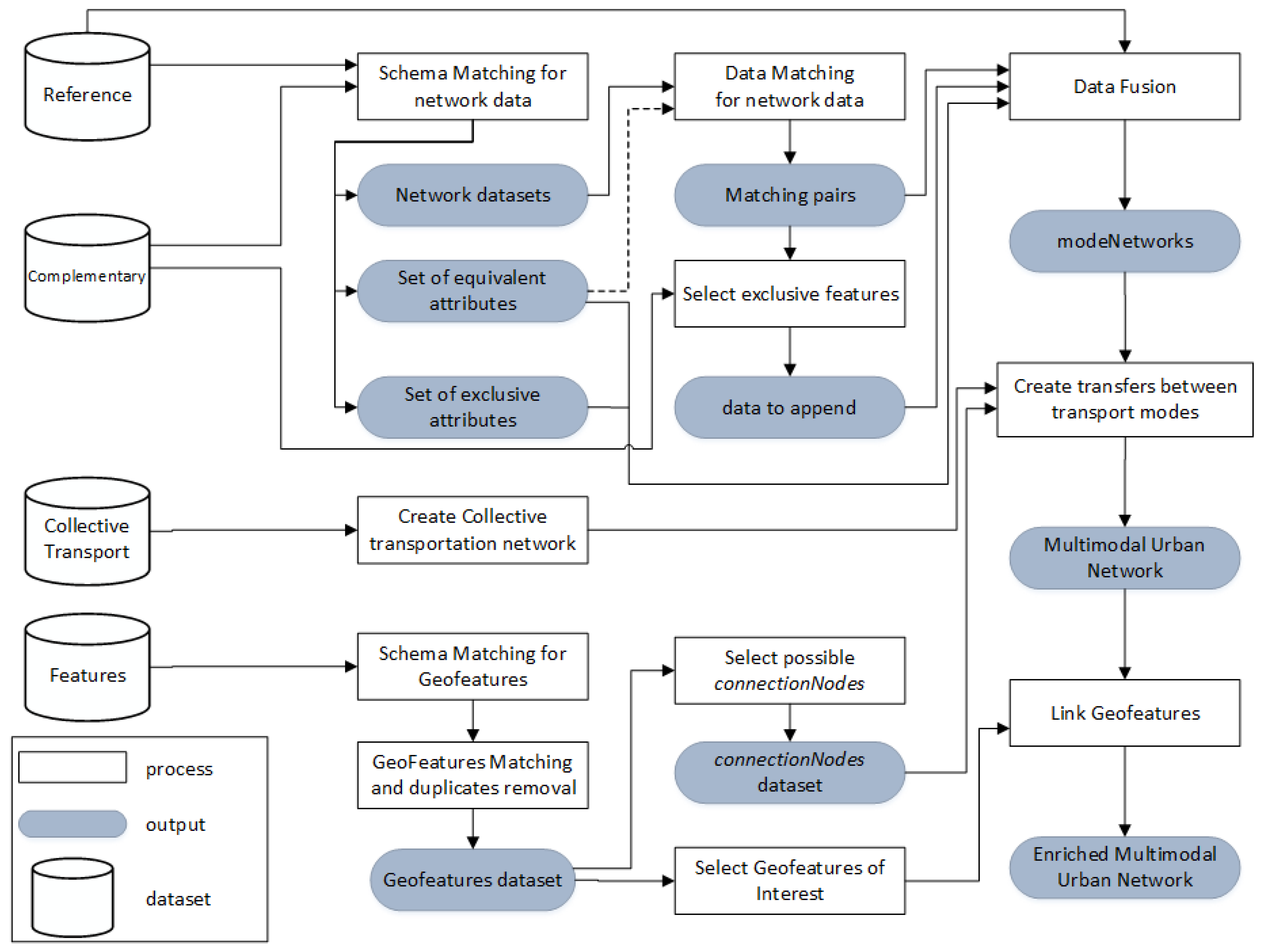
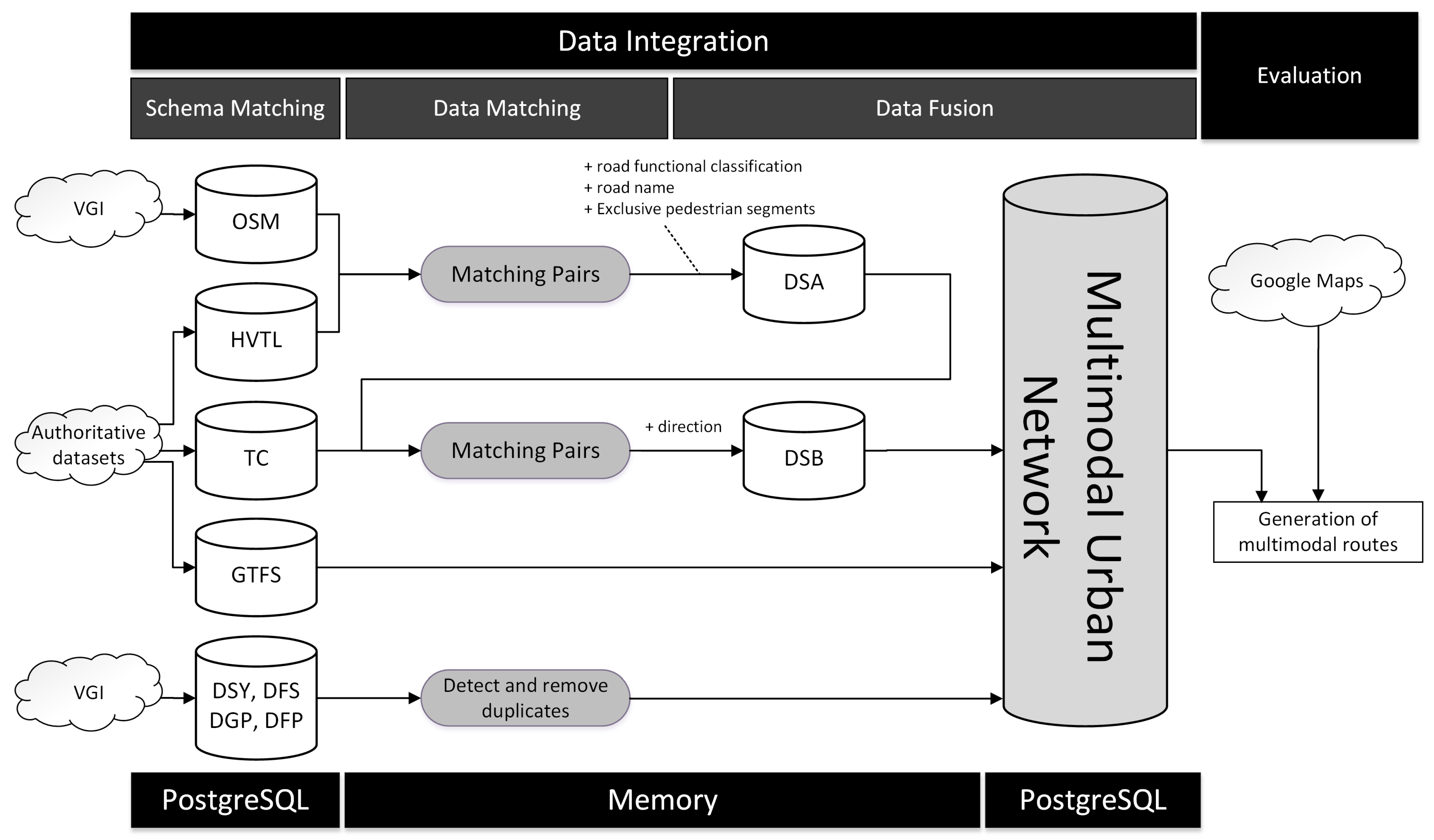
The first step to build a MUTN is the creation of a street network, which is used by pedestrians, bicycles and vehicles. This network is also where the components of collective transportation infrastructure are connected, and other GeoFeatures can be located. Our approach is to build the street network using data from different sources to get a more complete and up-to-date dataset, to use it as the basis to integrate data from public transport and other Geofeatures. An overview of the steps for building the multimodal network is shown in Figure 3. The remainder of this section presents each process in detail.

4.1. Initial Definitions

The following definitions are used in the description of the process:

• Reference Dataset: This dataset is the basis for the integration process and construction of the multimodal transportation network. It follows the proposed conceptual schema, and is the dataset whose data will be given preference when resolving data conflicts in data integration. Usually, but not necessarily, it should be an authoritative dataset.
• Complementary Dataset: contains data which can complement, expand, correct, or update the Reference Dataset.
• Collective Transportation Data: data related to routes, stops, and schedules of collective transportation infrastructure available at the same region of the Reference and Complementary datasets. The most common sources are GTFS files.
• Features Dataset: various datasets that can be used to enrich the resulting multimodal transportation network to enable its use in urban computing applications. This dataset provides features that are related to transportation mode transfer, such as parking lots or car sharing points, to enable multimodal routing.

4.2. Schema Matching for the Reference and Complementary Datasets

The MUTN schema proposed in this work establishes that a transportation network is represented as a directed graph. The first step of the work is to transform the reference and complementary datasets into a uniform graph representation, following the proposed schema. In the resulting network, each segment must begin and end in a junction. There must be a junction at every segment intersection if the transition from one segment to the other is possible. For example, in a street network, a road intersection must be a junction, but the point where a road (segment) intersects a tunnel or a bridge cannot be a junction since the transition is not possible.

Every junction must represent an intersection or a dead-end to match the MUTN schema. A cleanup operation should identify useless junctions, i.e., pass-through nodes that can be removed without altering the network’s topology. When such nodes are eliminated, the neighboring segments are geometrically merged. This operation can only be performed if the attributes of the neighboring segments are compatible. A set of attributes is considered compatible if it differs only in the values that relate to the geometry of the edge (e.g., length).

After the simplification process, two new properties are added (or updated) to the datasets, the length and the orientation of each segment. The length is the size of the segment’s geometry, in meters. The orientation of the segment is the angle, in degrees, from the source junction to the target junction considering east = 0, north = 90, west = 180, south = 270 degrees.

It must be possible to identify the mode (or modes) of transport for the segments in all datasets. Usually this information is stored as an attribute, else the entire dataset relates to a single transport mode.

Each dataset can have an arbitrary number of attributes for both segments and junctions. We opted to make manual matches in the case study, but existing semantic schema matching techniques can be used [88,89,90].

Finally, the last step is to transform all geometries to use the same coordinate reference system (CRS). The result of the schema matching are the graphs, $G_R$ and $G_C$, representing the reference and complementary datasets, respectively, with their attributes mapped to properties from the MUTN data model. The exclusive attributes from the complementary dataset are kept to be used, if necessary, in the data fusion process. The common attributes can be used in the data matching step to improve matching results by confirming or rejecting matching pairs based on available semantic information.

4.3. Data Matching for Network Data

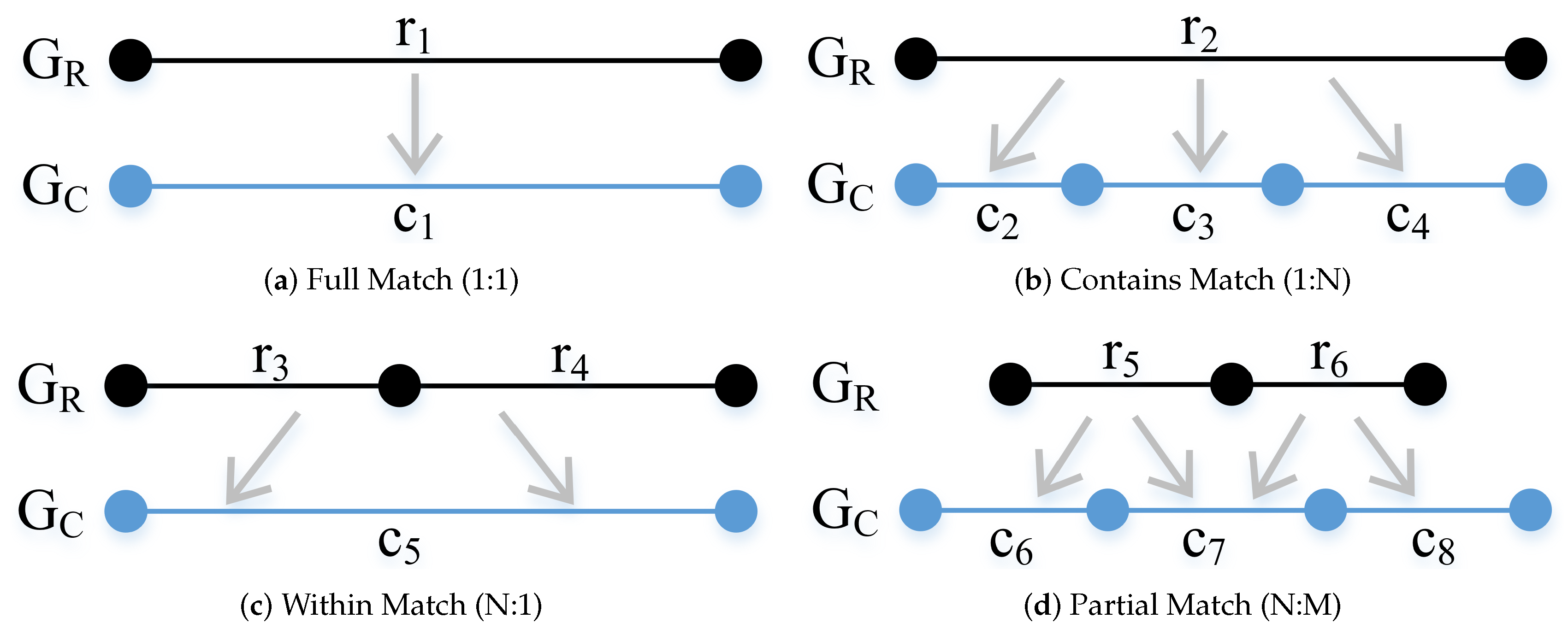
The data matching process works by finding matching pairs with increasing cardinality. We defined four cardinalities for the matching pairs: full, contains, within, and partial. Figure 4 shows in a simplified way the possible cardinalities for matching pairs. A fifth category, called null (one-to-zero cardinality), is used for features that have no match in the other dataset. This category is of fundamental importance for complementary data fusion, allowing one dataset to expand on the contents of the other to improve the completeness of the result. A full match (one-to-one cardinality), occurs when one segment from $G_R$ has an exact counterpart in $G_C$ and vice versa, which means that the source and target junctions of both segments are closer than a threshold and both geometries are similar. In Figure 4a, the segment $r_1$ from $G_R$ has a full match with segment $c_1$ from $G_C$. A contains match occurs when one segment of $G_C$ has the projections of its source and target junctions located at the same segment in $G_R$. In Figure 4b, the segment $r_2$ from $G_R$ has a contains match (one-to-many cardinality) with segments $c_2$, $c_3$ e $c_4$. A within match (many-to-one cardinality) is symmetrical to the contains match. It occurs when one segment in $G_R$ has the projection of its source and target junctions located in the same segment in $G_C$. Figure 4c shows that segment $r_3$ and $r_4$ from $G_R$ has within match with $c_5$ from $G_C$. A partial match (many-to-many cardinality) happens when the source and target junctions of a segment from $G_R$ has its projections in different segments in $G_C$ and correspondent segments in $G_C$ also cannot be related to one single segment in $G_R$. In Figure 4d segment $r_5$ has partial match with segments $c_6$ and $c_7$ from $G_C$.

The data matching process starts with a list of all possible candidate matching pairs ($L_{MP}$) from $G_R$ and $G_C$. Next, $L_{MP}$ is analyzed to find full matching pairs, then contains and within matches, and finally, the remaining non-matched edges are tested to find partial matching. If semantic information is available, an additional procedure can be triggered to check the reliability of the matching pairs found and to seek other possible matches in the non-matched edges.

4.3.1. Building the Set of Candidates for Matching

The first step in the process to find the list of all candidates for matching ($L_{PM}$) is to build an R-Tree based spatial index to accelerate the process. The index is created for the segments in $G_C$. Then, we search for nearby segments in $G_R$. Each segment in $G_R$ is buffered and used to search the index for segments in $G_C$ that intersect the segment’s buffer. All segments from $G_C$ that intersect the buffer are inserted in $L_{PM}$ along with the counterparts in $G_R$ as candidate matching pairs, with the following metrics: the difference between the segment orientations (in degrees) ($D_b$), the distance between the source junction of both segments ($D_{uu}$), the distance between the target junctions of both segments ($D_{vv}$), the distance between the source junction from $G_R$ and the target segment from $G_C$ ($D_{uv}$), the distance between the target junction from $G_R$ and the source junction from $G_C$ ($D_{vu}$), a flag indicating if the buffer of the segment from $G_R$ contains the candidate segment from $G_C$ ($B_{GT}$) and the length difference ratio ($L_{dr}$). All segments for which no candidate matching is found (a null matching) are marked as exclusive to the particular dataset and are not considered in the next matching steps, but it can be used in the data fusion process.

In the next steps, some metrics are calculated to guide the matching process. They are Node Proximity, Length Similarity, Angle Similarity.

Node Proximity

The node proximity is used to verify if the source and destination junctions of a segment r are close enough to the source and destination junctions of a segment c, considering distance tolerance, $t_d$. It is defined as:

$$P_{sim}(n_1,n_2)=\frac{dist(n_1,n_2)}{t_d}$$

(1)

where $n_1$ and $n_2$ are junction in the transportation network; $dist(n_1,n_2)$ is a function to calculate the distance between the two junctions, for example, Euclidean distance, and $t_d$ is the maximum distance to consider the two junctions as a possible match. There is no fixed value for $t_d$, as it depends on both datasets’ positional accuracy. For example, if both datasets have a high positional accuracy, a threshold of 5 or 10 m can be used to determine if a junction is close enough to the other. If the accuracy is low, it may be necessary to use a higher tolerance.

Length Similarity

The similarity by length considers that merely defining a tolerance based on a ratio of the difference in lengths is not appropriate. For example, if a segment $r_1$ is 20 m long and a segment $c_1$ is 16 m long they may match, even with the a 20% difference in length between them. However, if $r_1$ is 1000 m long and $c_1$ is 800 m long, possibly a 200 m difference is too high to consider them a match. The same principle applies if we only consider an absolute value for the difference. Suppose a difference of up to 40 m is used to consider two segments similar in length. In this case, a $r_1$ edge with 10 m and a $c_1$ edge with 50 m would be considered a match, which is not desirable. This way, lower and an higher absolute limits for the difference in length are defined, while intermediate values depend on the length difference ratio between the segments. The length similarity is defined as:

$$L_{sim}=\frac{\left|l_r-l_c\right|}{min(t_{lmax},max(t_{med},t_{lmin}))}$$

(2)

where

$$t_{med}=max(l_r,l_c)\times t_{ratio}$$

(3)

and $l_r$ and $l_c$ are the lengths of segments r and c, respectively. The $t_{lmax}$ and $t_{lmin}$ are the maximum and minimum absolute distance tolerance value, respectively; and $t_{ratio}$ is the tolerance value, in terms of the ratio between $l_r$ and $l_c$.

Angle Similarity

The angle similarity establishes if the difference of orientation angle of segments r and c is smaller than a threshold. It is defined as:

$$B_{sim}=\frac{\left|D_b\right|}{t_{bmax}}$$

(4)

where $D_b$ is the angle between segments r and c, and $t_{bmax}$ is the threshold difference (in degrees) to consider the orientation angle of both segments to be similar. For example, a $t_{bmax}$ of 15 degrees means that segments with angle differences up to 15 degrees are considered similar in orientation angle.

4.3.2. Finding Matching Pairs

The process of finding matching pairs works iteratively, searching for matches according to their cardinality. First, full matches are searched, then the contains and within matches, and finally the partial matches. Matching results are stored in hash lists keyed by the segment or junction ID for efficient retrieval.

A full matching occurs when one segment r in $G_R$, with $r_s$ and $r_t$ as source and target junctions, respectively, corresponds to exactly one segment c in $G_C$, with $c_s$ and $c_t$ as source and target junctions, respectively. The candidates list $L_{PM}$ is used to find full matching pairs, which are identified by checking if the values for length, angle similarity and node proximity, $P_{sim}(r_s,c_s)$ and $P_{sim}(r_t,c_t)$, are all less than or equal to one. The segments that satisfy this criterion are marked as a full matching. If a segment r has more than one candidate segment in $G_C$ for full matching, the one with the largest name similarity is chosen. In the case of a new tie, the candidate segment with the shortest distance is chosen. The candidate segments not chosen are available for new matching.

If a candidate pair fails the full matching test, the verification for the contains and within matching types occurs. A contains matching is established when one segment r from $G_R$ corresponds to one or multiple segments from $G_C$, and these segments in $G_C$ entirely fit the geometry of r, so we can say that r contains the segments from $G_C$. A segment pair (r, c), where $r\in G_R$ and $c\in G_C$, is a contains match if r strictly contains c, and the segment in r that corresponds to c (the projection of c in r) has $L_{sim}$ and $B_{sim}$ less than or equal to one. We defined that segment r strictly contains c if $c_s$ and $c_t$ have a valid projection in r, and, if the projection of $c_s$ in r is equal to $r_s$, then $P(r_s,c_s)$ must be less than one, and, if the projection of $c_t$ in r is equal to $r_t$, then $P(r_t,c_t)$ must less than one. An edge can have a within relation with only one other segment. When multiple candidates appear, the pair with the smallest distance is selected.

To find partial matches, we check if only one of the junctions of a segment c, $c_s$ or $c_t$, have a projection inside segment r. Considering $r^{\prime }$ as the part of r representing the projection of c in r, and $c^{\prime }$ the part in c representing the projection of r in c, if $r^{\prime }$ and $c^{\prime }$ have $L_{sim}$ and $B_{sim}$ less than than one, then r and c partially match each other.

4.3.3. Selection of Exclusive Features from the Complementary Dataset

After the matching process, the $G_C$ features that had no match (null matching) in $G_R$ are analyzed for a possible data fusion operation with $G_R$. This operation is also called conflation in the literature [34,61,76,91,92]. Merging one dataset’s exclusive data into the another allows complementing the data in the reference dataset and improving its coverage and completeness. The next section details the fusion process.

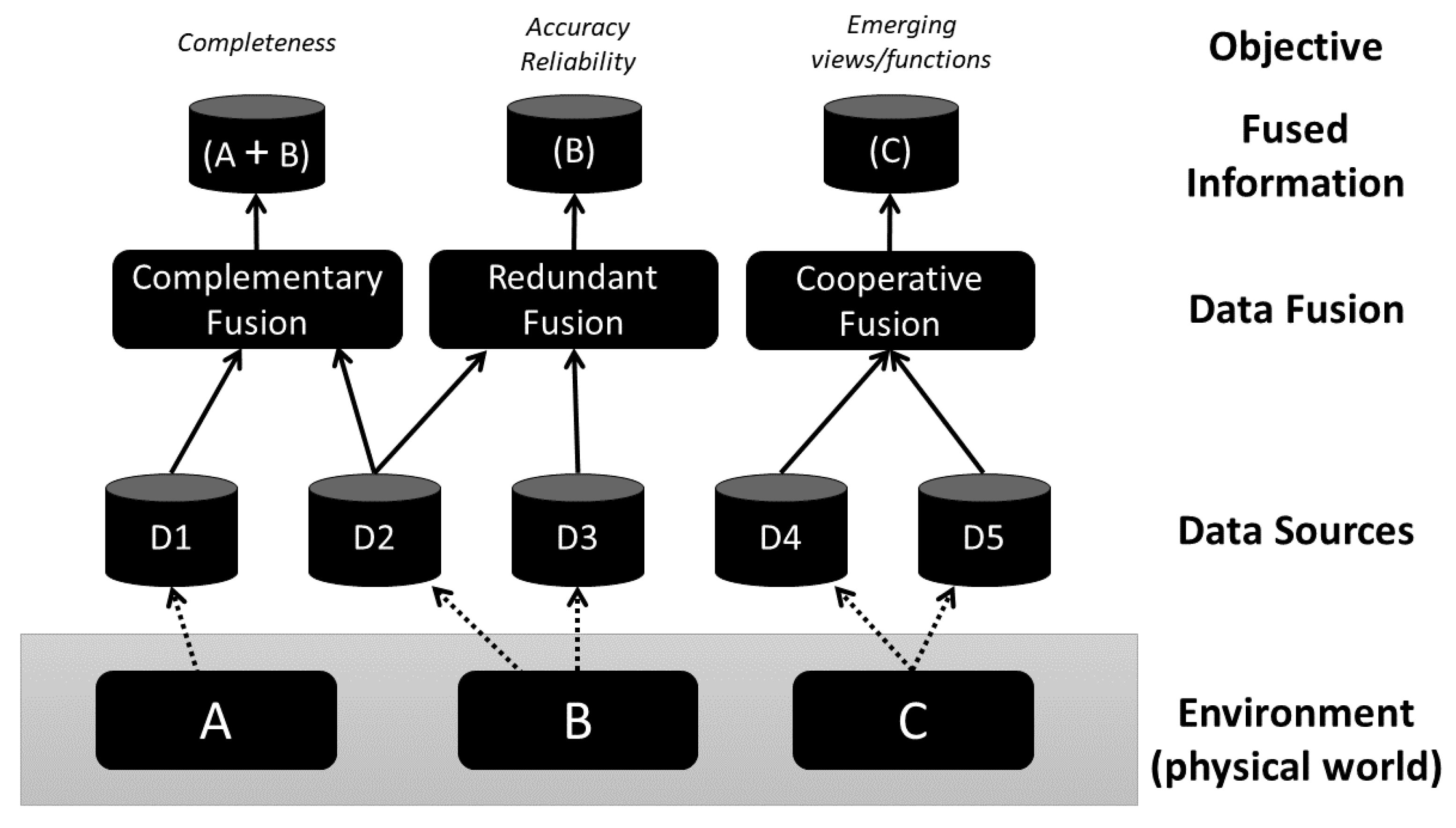
4.4. Data Fusion for Network Data

In this stage, the data fusion occurs in two ways: redundant and complementary. In the redundant data fusion, the matched features can have their attribute values updated. For example, if two road segments are matched, the value for a name attribute of one feature can be used to update the other. One problem that arises is how to define the attribute value of the feature resulting from the fusion of features. There is no single strategy, and cases may vary depending on the characteristics of the data sources and the purpose for the data fusion. When dealing with authoritative and crowdsourced data, the default strategy is to use the trust your friends technique from the conflict resolution category (see the data conflict taxonomy in Bleiholder and Naumann [85]) to give preference to the authoritative data source. If the value is not present in the authoritative data, a take the information strategy from the conflict avoidance category can be used to take the value available from other source, when available.

The complementary data fusion techniques are used to complement a dataset with features from other datasets without a correspondence (null matches). In this case, a fully automated process is complex and may be subject to errors that must be verified by humans. In this work, the complementary fusion at this stage is used in two situations: missing driving directions information and inclusion of connected segments for which no match was found.

To detect missing driving directions, the road segments for which there are matching candidates that could not be matched are analyzed. If, for instance, there is a mismatch due to the angle similarity metric, and the angle difference is close to 180 degrees, then the segment is considered an erroneous driving direction, and a new segment is inserted.

The data fusion process to include sets of connected segments that did not match checks if there are any connections of previously matched segments to any segment from the set. If connections exist, they are inserted in the reference dataset and connected. Otherwise, the junctions in the set closer than a distance tolerance ($t_d$ as default) from a junction or segment in the reference dataset are connected. The new segments created to connect the sets of segments receive a flag ‘needs_review’ to indicates they need further validation.

4.5. Creation of the Collective Transportation Network

The creation of a collective transportation network dataset has particularities that must be taken into account. First, unlike individual transportation networks, collective transportation routes are defined with a specific schedule. Second, the actual physical path taken by a vehicle in collective transportation is not always available; however, it is possible to collect data regarding the lines and their sequence of stops. A currently adopted standard for collective transportation information dissemination is GTFS files.

The proposed data model allows building a public transport network with pre-defined routes through Connection Node, Route, RouteSegment, and Timetable classes by mapping GTFS data to the proposed schema. A Route stands for a path through a sequence of collective transportation stops. Each stop is represented as a ConnectionNode as they allow a change in the mode of transport (WALK→BUS). The GTFS file allows the grouping of stops in stations. When building the collective transportation network for the proposed data model, the same station’s stops are unified in the same ConnectionNode represented as a station. When leaving a route, the user can change the transport mode (BUS→WALK) or make a connection to another route (BUS→BUS). To enable inter and intra-modal routing, each ConnectionNode used by several routes is duplicated (one for each possible route), and TransferSegments of type InterTransfer are created to enable the assignment of a cost when a collective transportation user makes the connection. The connection of ConnectionNode to the individual transportation network is made according to the possible mode of transport. Generally, the collective transportation network will be connected to the pedestrian (street) network through TransferSegments of type OuterTransfer. For each RouteSegment, the corresponding Timetable is created containing the information of days and times of arrivals and departures of a vehicle traveling along a certain route.

4.6. GeoFeatures Matching and Duplicates Removal

Geofeatures can appear in the MUTN data model as points, lines, or polygons. The task of consolidating data from different sources for the features is complex. For example, Geofeatures represented as points have no geometric attributes that can identify duplicates beyond their position. Therefore, the use of semantics in the matching process is always necessary. Even so, the task remains hard to be fully automated because features have different sets of attributes, attributes that represent the same information appear with different names or data types, attribute values may be in different languages, among other challenges related to automated schema matching. In this work we only deal with PointFeature matching.

To identify duplicates, the strategy is to compare PointFeatures close to each other at an arbitrary tolerance distance and with similar names (all GeoFeatures must have a value for the name property, null values are not allowed). The Levenshtein distance is a widely used similarity metric to compare names. However, its results are sensitive to the order in which the words appear in the strings, to punctuation, and to lowercase or uppercase letters. For example, a place $p_1$ named “Capitólio Estacionamento” and another $p_2$ named “Estacionamento Capitolio” has a normalized Levenshtein similarity of 0.58. Crowdsourced data has great variability in the attributes whose values the user can provide freely. To minimize this variability and improve the matching results, we pre-process the names before using the Levenshtein distance. First, the names are converted to lowercase characters, and the punctuation is eliminated by tokenizing the strings. The tokens are then sorted alphabetically and concatenated. Then the Levenshtein distance is calculated and normalized. The name similarity, $N_{sim}$, can be expressed as Equation (5):

$$N_{sim}(p_1,p_2)=\frac{(length(p_1.nam{e}^{\prime })+length(p_2.nam{e}^{\prime }))-levenshtein(p_1.nam{e}^{\prime },p_2.nam{e}^{\prime })}{length(p_1.nam{e}^{\prime })+length(p_2.nam{e}^{\prime })}$$

(5)

where $length$ is a function to return the number of characters of the string representing the name of the PointFeature, and $nam{e}^{\prime }$ represents the processed $name$ of the feature after conversion to lowercase characters, tokenization, sorting and concatenation. Applying $N_{sim}$ to the previous example of $p_1$ and $p_2$ results in a value of 0.98.

PointFeatures $p_1$ and $p_2$, with the same FeatureClass that are close enough to each other and have similar names according to a given tolerance ($t_{name}$), are considered to be duplicated. If $P_{sim}(p_1,p_2)$ (Equation (1)) is less than than one, $p_2$ is automatically considered a duplicate. If not, those points that names have $N_{sim}(p_1,p_2)$ with value of $t_{name}$ or more are considered duplicates until a distance up to $d_m$ (distance multiplier) times the $t_d$ (distance tolerance). Formally, the $isDuplicate(p_1,p_2)$ function is defined as:

$$isDuplicate(p_1,p_2)=\left\{\begin{array}{cc}true,\hfill & \mathrm{if}\left(P_{sim}(p_1,p_2)\le 1\right)\mathrm{or}\left(P_{sim}(p_1,p_2)\le d_m\mathrm{and}{N}_{sim}(p_1,p_2)\ge t_{name}\right)\hfill \\ false,\hfill & \mathrm{otherwise}.\hfill \end{array}\right.$$

(6)

4.7. Selection of ConnectionNodes

ConnectionNodes are selected from the GeoFeatures. To create the multimodal transportation network, we select GeoFeatures types that can be used to change the mode of transport. For example, parking lots can be used in the transition from car to rail transport mode, and vice versa.

4.8. Creation of Transfers between Transport Modes

The points to be used as ConnectionNodes are classified according to the mode of transport from which a transition in and out can occur. For each set, connections are created by looking for the Junction closest to the position of the ConnectionNode and creating a TransferSegment of type OuterTransfer. For example, a set of ConnectionNodes that will be used to transition from DRIVE to WALK will be connected to the DRIVE network via an incoming OuterTransfer and to the WALK network via an outgoing OuterTransfer segment.

4.9. Linking GeoFeatures to the Multimodal Urban Transportation Network

The MUTN data model allows us to store GeoFeatures for different applications. For those that are not directly related to routing, it is not necessary to create Junctions for them. Instead, the GeoFeatures are created, and the class NetLocation is used to store where in the transportation network a GeoFeature can be reached. This way, the MUTN data model is kept stable without excessive partitioning of the segments to create links to GeoFeatures.

5. Case Study

To test the validity of the framework, a multimodal urban transportation network for the Brazilian city of Belo Horizonte was built. Data from different sources were used and integrated to allow the creation of multimodal routes. Official (reference) and alternative (complementary) datasets were used. Datasets were considered official if their provider is an agency connected to the public administration, otherwise they were considered to be alternative. First, the datasets’ schemas were mapped to the MUTN proposed schema. Second, datasets were integrated using data matching and fusion techniques to build the individual transportation network dataset. Then, GTFS files were used to build the collective transportation network dataset. Finally, data from additional and heterogeneous sources were integrated to establish ConnectionNodes between modes of transport. The resulting multimodal urban transportation network was used to find routes among eighty points using DRIVE, WALK, and TRANSIT transportation modes. The routes created were then compared against the equivalent Google Maps routes. The experiments were conducted on a laptop computer with Intel Core i5-9300H processor, 1TB hard disk, 20 GB RAM, PostgreSQL 11.7 (64-bit) with extensions PostGIS (3.0.1) and hstore (1.5) enabled. All the methods were implemented using the Python (3.8.5) language. Figure 5 shows an overview of the procedures executed in the case study.

The remainder of this section describes the datasets used in the case study, and explains how they were integrated to build the MUTN. Section 6 discusses the results.

5.1. Datasets

5.1.1. Alternative Datasets

This work used data from OpenStreetMap, Yelp, Foursquare, Google Places and Facebook Places as alternative datasets.

OpenStreetMap (https://www.openstreetmap.org/ (accessed on 21 june 2021)) (OSM) is a crowdsourced mapping platform to which any person in the world can contribute. OSM data are represented by only three different types of objects: nodes, ways, and relations. A node represents a geographical point. It has, at least, an ID number (osmid) and the geographical coordinates as latitude and longitude values (EPSG = 4326). A way represents linear features (streets, rivers) or area boundaries (buildings, forests, lakes) and is formed by an ordered list of between 2 and 2000 nodes. When the way represents an area boundary, the first and the last nodes have to coincide spatially. The area can be solid (e.g., a building) or not (e.g., a roundabout), and the tags associated with the way have to be examined to define its type. Relations represent a relationship between two or more other OSM elements (nodes, ways, or other relations). For example, an area boundary with a hole can be represented as a relation between two ways representing areas. A relation is an ordered list of the objects it contains, which are called the relation’s members.

Attributes in OSM use a free tagging system that allows the inclusion of an unlimited number of attributes to each feature. This system is very flexible, but makes querying and manipulating data harder [13]. The tags are organized as key-value pairs, but there is no formal convention to use them. Informal rules emerge from community usage, in the form of agreements to use some keys and values to describe specific elements. Frequently, the community of contributors draws up proposals to approve new tags, but this not guarantee their proper or universal use. In the end, the “crowd” defines what and how to use these elements.

OSM data was downloaded from Geofabrik (https://download.geofabrik.de/south-america/brazil/sudeste.html (accessed on 7 July 2020)), a service that hosts OSM extracts for several regions. Data used in this case study represent a snapshot from 1 July 2020. The data was clipped to include only the objects inside the polygon representing Belo Horizonte’s city boundary. However, looking at the collective transportation data, several points along bus routes fall outside the official city limits. This way, we used a buffered version of the polygon (it was necessary to expand the original polygon in 1200 m) to clip the original data. The resulting OSM dataset representing the road network includes 33,348 road segments totaling 7,053,116 m.

Facebook Places (DFP), Google Places (DGP), Yelp (DYP), Foursquare (DFS) and OSM (DOP) were used as sources for points of interest. All services provide APIs for data queries. However, there are limitations on the volume of queries that can be executed at a given time (for DFP, DGP, DYP and DFS). The collection was assembled by querying reference points 25 m away distributed as a grid across the available area. Data for each service were cleaned to eliminate duplicates (see Section 4.6) and stored. For instance, the number of points representing parking lots was initially 1613. After cleaning and elimination of duplicates, the total count dropped to 1238 (

Table 1. The number of points and lines from datasets before and after schema matching procedures.

Dataset	Raw Data		After Schema Matching
	Points	Lines	Points	Lines
TC	146,542	231,112	145,625	125,554
HVTL	—	54,354	40,287	111,740
GTFS	9328	—	35,250	322,122
OSM	123,308	260,265	47,458	127,656
DOP (OSM-parking lots)	317	—	49	—
DGP (Google Places)	918	—	857	—
DFP (Facebook Places)	6	—	5	—
DSY (Yelp)	52	—	31	—
DSF (Foursquare)	320	—	296	—

). Facebook Places and Yelp contributed with a relatively small amount of data. However, some of them were unique, and so we chose not to remove them from the data integration process to get a more complete result.

5.1.2. Official Datasets

Four official datasets were used. The first dataset, called “Classificação Viária” ($HV$), stores data about functional classification for each road segment. The second dataset, called “Trecho Logradouro” ($TL$), contains the name of each road segment. These two datasets have relational integrity constraints defined, thus it is straightforward to join information of both datasets using relational database operations ($HVTL$). The third dataset, called “Circulação Viária” ($TC$), has data about the city street network. Each segment is related to an origin and a destination node. Street data corresponds to a directed graph using two edges to represent two-way streets, which causes many duplicate nodes at intersections, used to represent turn permissions. There is no way to link a segment in $TC$ to a segment in $HVTL$ only using attribute values, so it is necessary to use spatial data matching operations to integrate the data from both datasets. All three datasets are part of Belo Horizonte’s Spatial Data Infrastructure (http://bhmap.pbh.gov.br/ (accessed on 9 July 2020)), created and managed by the city’s administration.

The fourth dataset is the set of GTFS files provided by the city’s traffic department, BHTrans (https://dados.pbh.gov.br/dataset/gtfs-estatico-do-sistema-convencional (accessed on 3 July 2020)). The data used is from 29 July 2020, has 9328 stops, 643 routes, 56,771 trips, and 3,202,454 timetable entries for each trip at each stop. Table 1 shows an overview of the number of point and line objects gathered from official and alternative datasets and the results after schema matching procedures.

5.2. Schema Matching Procedures

The schema matching process starts by creating a directed graph representation of the datasets to match the proposed MUTN schema. The $TC$ dataset is already in the proper format, since it has a segment for each direction, and each segment has a source and destination junction. However, $TC$ dataset has segments that do not follow the physical counterpart in real world, which are used to represent the allowed turns between segments. These segments were used to build the $TC$ network, but were not considered in the data matching process. After schema matching, the $TC$ dataset had 145,625 nodes (junctions) and 125,554 lines (segments) (Table 1).

The network structure to represent $HVTL$ had to be built, since only the segments’ geometry was available. A junction was created for each segment intersection and the respective segments received the attributes for their source and target junctions. There was no information to infer the traffic flow in $HVTL$. This dataset was used primarily to transfer information about road functional classification, road names and exclusive pedestrian segments to the MUTN data model. After schema matching the $HVTL$ dataset had 40,287 points (junctions) and 111,740 lines (segments) (see Table 1).

OSM data required some transformations to match the MUTN data model. Road segments representing two-way streets in OSM were duplicated and inverted to create two one-way segments. An OSM way feature was considered oneway if it has a tag oneway with any of the values: yes, true, 1 or −1. In the case of value −1, the direction of the segment was reversed. Source and target junctions are not readily available in OSM dataset. Each way in OSM has a nodes attribute, which is an ordered list of all node codes that compose the way’s geometry. OSM graph is first constructed using all nodes and then is simplified to eliminate intermediate nodes following the procedures described in Section 4.2. After schema matching the OSM dataset had 47,458 points (junctions) and 127,656 lines (segments) (see Table 1).

Data from Foursquare, Google Places, Facebook Places, OSM, and Yelp were selected from their respective datasets, filtering only those that corresponded to parking locations. We manually identified the attribute values needed to filter the data in each dataset correctly. For example, the data in OSM was filtered using the tag value amenity = parking. The resulting number of points from each dataset is shown in Table 1.

5.3. Data Matching and Fusion between OSM and HVTL

The data matching procedure find corresponding pairs of segments in the datasets. First, the matching is done between OSM and HVTL datasets following procedures presented in Section 4.3.2. The resulting matching pairs are used to fuse the data between the datasets. The OSM dataset contributed with information about the mode of transport allowed in each segment (derived from the tags). The HVTL dataset was used as a source for checking the information of the segments’ names and functional classification. It was also used as a source of additional pedestrian segments.

Table 2. Number and length (meters) of segments matched between OSM and HVTL datasets.

	OSM				HVTL
	Count	%	Length	%	Count	%	Length	%
full	49,010	38	4,620,917	37	49,010	44	4,624,037	49
contains	10,055	08	1,565,083	12	7805	07	1,004,634	11
within	9877	08	740,788	06	18,113	16	1,000,159	11
partial	18,678	15	1,776,123	14	21,495	19	1,939,919	21
Matched	87,620	69	8,702,913	69	96,398	86	8,568,751	92

shows the number and total length (in meters) of segments in each dataset that were matched discriminated by the type of matching. This information can characterize the potential of each dataset to contain complementary or redundant data relative to the other, but does not show whether the matches are correct or not (see Section 5.5). Approximately 69% of the segments and total length of OSM and 86% of the segments and 91% of the total length of segments in HVTL were matched. The high rate of segments and length matched in HVTL indicates that it will contribute mostly as redundant data in the data integration process, while OSM has more complementary information to contribute.

Once the matching pairs have been established, the fusion procedure for the datasets takes place. Three attributes were used in the fusion process: width, level, and name, which represent the width, functional classification, and the segment name, respectively. OSM dataset had few segments with width value (115). In this case, the fusion strategy was to rely on data from the HVTL dataset. In case of difference in values, if the same segment is involved in more than one matching pair, the new value for width is calculated by averaging the values found. A total of 87,532 segments had their width value assigned or updated.

During the schema matching phase, each dataset’s attributes representing the level value in the MUTN data model were mapped to corresponding values.

Table 3. Value mapping for attribute ‘level’ in the segments of the MUTN data model.

MUTN	OSM	HVTL
Level	Highway	Desc_Class
1	residential, unclassified, service, services, construction, corridor, crossing, cycleway, disused, dummy, footway, industrial, living_street, path, pedestrian, steps, track	local
2	secondary, secondary_link, tertiary, tertiary_link	coletora
3	primary, primary_link	arterial
4	motorway, motorway_link, trunk, trunk_link	ligação regional

shows the correspondences in the values. In the OSM dataset, the values in the table represent the contents of the ‘highway’ tag for the segments. In the HVTL dataset, the values represent the contents of the ‘desc_class’ attribute. The fusion strategy adopted was to consider the lowest level in case of disparity to prevail over the most restrictive classification in terms of speed allowed in the segment. At the end of the process, 2553 segments had their level values updated.

The OSM dataset has 3438 segments with no value for the name attribute among those with a corresponding pair. When merging the name attribute, a strategy was adopted to update the values only when the corresponding pair’s value had a similarity below 80% (Equation (5)). In this case, the name value of the dataset HVTL was preferred, since it is an official source (Trust your friend fusion strategy). For partial or contains matching, the HVTL dataset values were considered only when more than 50% of the segment length was matched. At the end of the process, 2813 segments had new values for the name attribute, and 10,599 segments were updated.

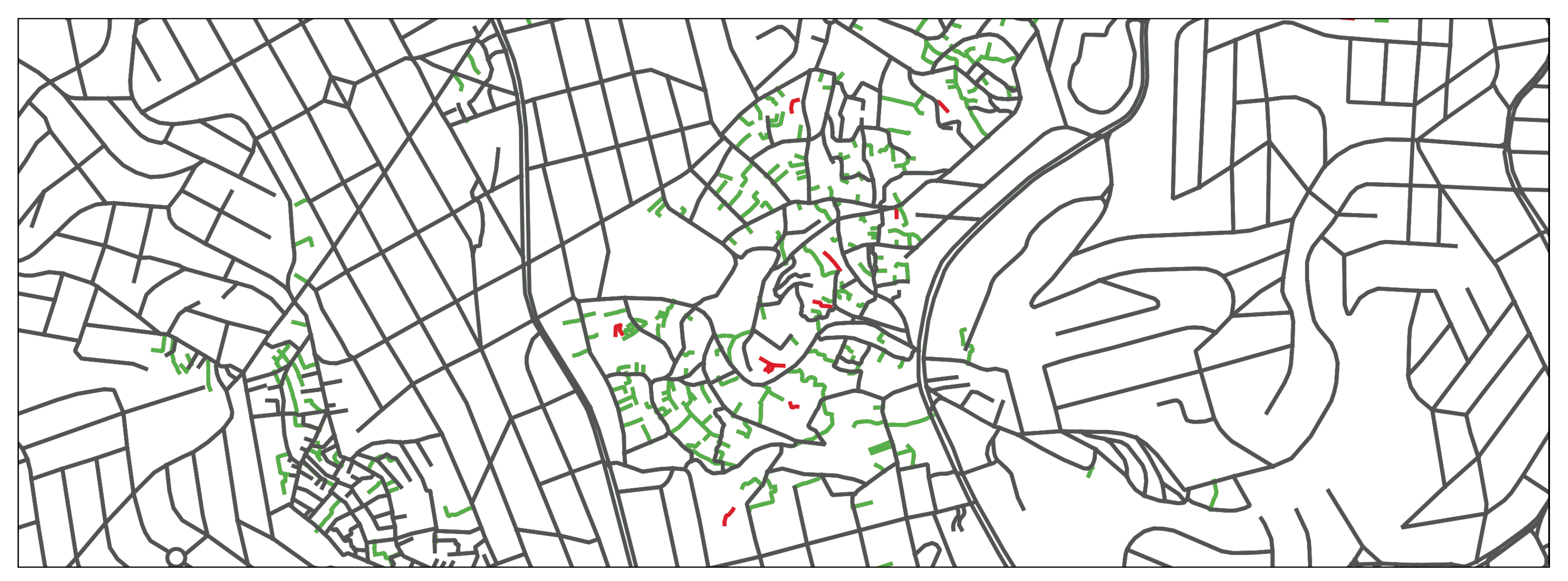
The last procedure in the fusion between OSM and HVTL datasets was the insertion of exclusive pedestrian segments from HVTL. The segments were identified by the attribute values ‘tipo_lograd’ equal to ‘VIA DE PEDESTRE’ (walkway), ’BECO’ (alley), or ‘TRAVESSA’ (a narrow cross-street). Even if some of these segments could be used for motor vehicles, they were considered only for pedestrian use. There was not enough information in the HVTL dataset to guarantee, for example, whether or not a segment could be used by cars and which would be its correct driving direction.

In the fusion strategy, the exclusive pedestrian segments in HVTL that did not match with one in OSM were grouped into connected components. For each connected component, Junctions were detected that were within a tolerance distance of some segment of the OSM dataset. If it exists, the respective segments are connected, and the entire group is integrated. If not, all the connected component is disregarded. Figure 6 shows segments from OSM dataset (in black) and the segments from HVTL that were successfully integrated (in green) and the ones that were dismissed (in red). In this process, 5591 HVTL segments were found grouped into 1219 connected components. The resulting dataset from the fusion was named DSA and had 136,675 segments, 51,179 junctions, and a total length of 12,694,791 m.

5.4. Data Matching and Fusion between DSA and TC

The integration between DSA and TC follows the same procedures used in the fusion between OSM and HVTL. First, the matching pairs are found. At this stage, only the DSA segments (DSA${}_d$) that allow motor vehicles were considered since in the dataset TC there is only this type.

Table 4. Number and length (meters) of segments matched between DSA${}_d$ and TC datasets.

	DSA${}_{\mathit{d}}$				TC
	Count	%	Length	%	Count	%	Length	%
full	4346	4	294,352	2	4346	3	273,233	4
contains	57,320	47	6,375,217	53	2697	2	396,296	5
within	3836	3	209,065	2	64,461	51	5,132,231	68
partial	12,131	10	1,051,726	9	49,777	40	1,528,043	20
Matched	77,633	64	7,930,362	66	121,272	96	7,329,804	97

shows the number and total length (in meters) of segments that were matched between the DSA${}_d$ (only segments for motor vehicles) and TC datasets, discriminated by the type of matching. Approximately 64% of the segments of DSA${}_d$ and 96% of the segments in HVTL were matched. DSA${}_d$ had most of the matched segments of type contains, which is in line with the high rate of within matches in the TC dataset. The results indicate a more significant fragmentation of TC segments, but the high overall rate of matched segments suggests it is a source of redundant data to the data integration process. These matching results shows that correspondences were found among the segments of the dataset, but does not confirm if it was correctly matched or not. Section 5.5 presents the quantitative evaluation of the matching process to assess the quality of the matchings.

Once the matching pairs were found, they were used to check the driving direction in DSA${}_d$. For this purpose, we analyzed all the segments in DSA${}_d$ that had a match, but that their equivalent in the opposite direction did not. Using this approach 1300 segments with the incorrect direction were found and removed from DSA${}_d$. The DSA dataset, with the removal of the segments in the wrong driving direction, was named DSB.

5.5. Quantitative Evaluation of Data Matching Results

To quantitatively evaluate the data matching process, we conducted a manual matching of a random sample of 400 features for each process, OSM-HVTL and DSA${}_d$-TC, and compared the respective results This sample size gives us a 95% confidence interval with less than 5% margin of error. The samples were selected in QGIS using the random selection tool. Then, each selected feature was manually matched by visual inspection. The results were then compared with the data matching processes for OSM-HVTL and DSA${}_d$-TC. Two evaluation metrics were used, precision and recall, defined by Equations (7) and (8):

$$precision=\frac{TP}{TP+FP}$$

(7)

$$recall=\frac{TP}{TP+FN}$$

(8)

where True Positive ($TP$) is the number of segment pairs corrected matched. False Positive ($FP$) is the number of segment pairs wrongly matched. False Negative ($FN$) is the number of segment pairs missed by the data matching process. The intuition is that precision relates to the correctness and recall to the completeness of matching.

The data matching process between OSM and HTVL had a precision of 97.7% and recall of 96.7%. The results for the matching between DSA and TC was of 98.2% and 97.7%, for precision and recall, respectively.

5.6. Creation of the Collective Transportation Network from GTFS

Although OSM can represent the geography of collective transportation, it lacks information to be effectively used for route planning. For example, OSM data has only 1457 bus stops (nodes with tag highway = bus_stop), while GTFS data for Belo Horizonte has 9328 stops. Furthermore, although there are some proposals to store timetable data in OSM, it is not clear if the community will embrace it, since it violates some principles on not including temporal and seasonal features. Hence, we rely on GTFS data to build the collective transportation transport network dataset to be integrated into MUTN.

The processing of GTFS files for Belo Horizonte follows the steps described in Section 4.5. For each stop-route combination, a Junction is created. Then, TransferSegments are created to connect each Junction, which represents the same stop. This way, we can create TransferSegments between the routes.

For each segment of a route, a transition between two stops, a RouteSegment, is created. Each RouteSegment has an associated timetable object with all departure times assigned to that route between the two stops (in GTFS, this is represented as a trip). It is common that the GTFS files do not to have the complete departure time data for each stop, since it is only mandatory for them to be present at the first and last stop. In this case, each stop’s estimated departure time was interpolated using the total time spent on the route by the number of stops. Then, each timetable object of each TransferSegment between ConnectionNodes representing collective transportation stops is fulfilled with all departure times from one stop to another and the traversal time (in seconds).

A collective transportation stop is where a change in transportation mode can occur, which means it is a ConnectionNode in the MUTN. This way, each stop is connected to the closest segment that allows the pedestrian transportation mode. TransferSegments are created, both inbound and outbound, for each ConnectionNode and its nearest pedestrian segment. The numbers resulting from creating the collective transportation network for the MUTN were shown in Table 1. The total number of ConnectionNodes was 35,250, and TransferSegments was 322,122.

5.7. Integration of ConnectionNodes into MUTN

The creation of ConnectionNodes used data from five datasets: OSM (DOP), Yelp (DSY), Facebook Places (DFP), Google Places (DGP), and Foursquare (DSF). The points from all datasets identified as parking lots were selected. In the case of DOP, it is possible to find parking lots also represented using area features. For them, a point inside the area is automatically generated to represent the parking lot as a ConnectionNode.

The integration of the points uses two criteria (as seen in Section 4.6): the node proximity and the name similarity. For the case study, we used a distance tolerance ($t_d$) of 5 m. So, if two points were less than or equal to 5 m from each other, they were considered to be duplicates. Else, up to 20 m ($d_m=4$, which means four times the tolerance), the name similarity ($N_{sim}$) is executed, and any two points with a similarity of 0.8 ($t_{name}$) or more are considered to be duplicates. The values for $t_d$, $d_m$, $t_{name}$ were determined empirically.

After processing, 1238 ConnectionNode were created. The integration of these points into the MUTN was made using information on the possibility of change of transport mode at the TranferJunctions. We considered the parking lots as a local to change from DRIVE (motorized vehicles) to WALK (pedestrian). For each one, we identify the nearest segment with transport mode DRIVE and connect them with a TransferSegment of type OuterTransfer (DRIVE → ConnectionNode). Similarly, we find the nearest segment with transport mode WALK and connect to the ConnectionNode (ConnectionNode → WALK).

After this integration step, the MUTN is almost complete, and is necessary to associate traversal costs for the segments to enable calculation of multimodal routes. Our approach was to use the time in seconds to traverse the segment as the default cost.

5.8. Cost Assignment to Segments

The maximum speed and segment length are required for the cost calculation. Only 5.72% of the segments have a value for the maximum speed assigned. For segments that do not have an assigned value, a default value is derived from the segment’s functional classification (level). The Brazilian traffic code (http://www.planalto.gov.br/ccivil_03/leis/L9503Compilado.htm (accessed on 7 August 2020)) establishes four different classifications for urban roads: fast, arterial, collector, and local traffic. Each of them has a maximum speed of 80 km/h, 60 km/h, 40 km/h, and 30 km/h, respectively, if there is no signal indicating otherwise. If there is already a speed indication for the segment, the lowest value is used. However, a vehicle does not move at maximum allowed road speed all the time, and there are many variables that affect its speed, such as type of vehicle, time of day, weather conditions, and school hours. We adopted a value of 65% of the maximum speed for the cost calculations. This value is an estimation based on radar data from BHTrans (https://dados.pbh.gov.br/dataset/contagens-volumetricas-de-radares (accessed on 7 August 2020)).

For pedestrians, an average walking speed of 4.8 km/h was used [93]. The segments for collective transportation already have time in seconds of transition between their points defined in GTFS files. These values were used as the cost of the segments. For segments that represent transfer between routes in collective transportation (InterTransfers), a cost of half of the interval between departures on the destination route was used. For the study case, only parking lots were used as possible points to change the mode of transport between DRIVE and WALK modes (OuterTransfers). The time spent to park a car varies widely depending on location and time of day, and it is difficult to estimate it accurately [94,95]. For the case study, we empirically set a cost of 300 s when a transition happens.

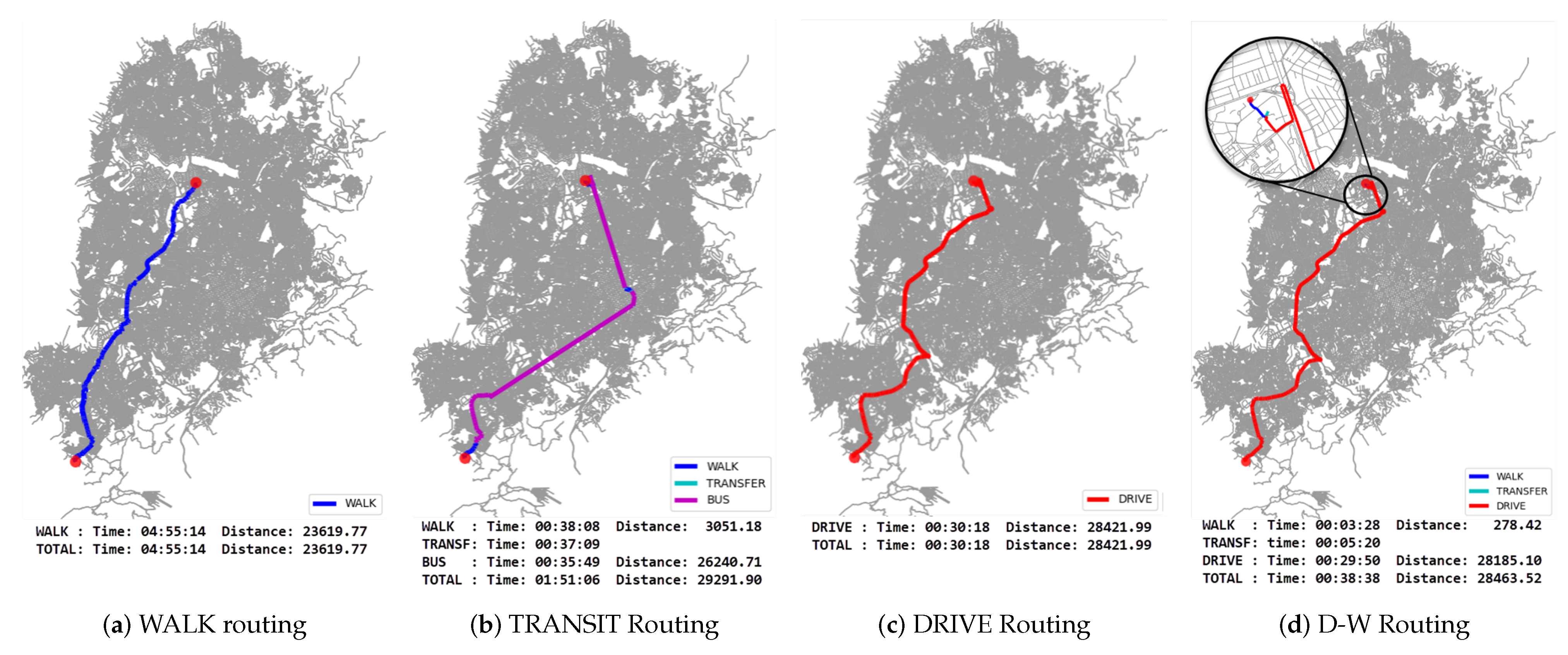
5.9. Multimodal Routes Using the MUTN

After the segment costs were defined, the MUTN had all the necessary information to generate routes using different transport modes. In the case study, the possible transitions between transport modes are from walking to collective transportation (and vice versa), and private vehicle to walking. The first is the typical situation of a collective transportation user who walks to a station or stops, takes a bus, and possibly changes lines until the end of their journey. The second case considers a driver who needs an appropriate place to park their vehicle near the destination.

The possibility of stopping the vehicle on the streets was not considered, only in specific parking lots. We consider that parking on the streets is already contemplated by the transportation mode, considering only the private vehicle (although a time penalty may be applied according to the expected time to find a parking spot near the destination). Therefore, the MUTN for Belo Horizonte supports routing for DRIVE, WALK, TRANSIT, and D-W (drive and walk) for the modes of transport of private vehicle, pedestrian, collective transportation, and private vehicle with the need for parking and walking to the destination, respectively.

Dijkstra’s algorithm was used to determine optimal MUTN routes based on the segment costs. Figure 7 shows examples of routes created in the MUTN network considering DRIVE, WALK, TRANSIT, and D-W modes between the same points (Origin: (600,421.4768275785, 7,784,595.199524326); Destination: (608,600.8233442156, 7,803,574.252453946); EPSG:31,983).

6. Results and Discussion

To compare the results obtained by modeling and integrating the data, we created routes between 80 points spread throughout the municipality area. Each point represents a location at the MUTN closest to the centroid of each of Belo Horizonte’s planning units. Planning units are territories formed by the aggregation of census sectors, used by the public administration in various situations, such as calculating socioeconomic indicators (e.g., urban life quality, social vulnerability), and distributing participatory budget resources.

Routes between all pairs of points were calculated for the WALK, DRIVE, TRANSIT transport modes using MUTN, and Google Maps. Google Maps does not have an option for car routes looking for parking near the destination, so it was impossible to compare it with the D-W routing option.

For each route, the time and the distance were calculated using MUTN and Google Maps. Then, the differences between distances and times were calculated, and finally, the ratio between the differences and the respective values obtained by MUTN.

Table 5. Comparison, by time and distance, between the routes created using the Multimodal Urban Network and Google Maps. Values represent the average of the absolute ratio difference.

Distance Range (m)	WALK		DRIVE		TRANSIT
	dist_diff	time_diff	dist_diff	time_diff	dist_diff	time_diff
	(%)	(%)	(%)	(%)	(%)	(%)
(0, 3486]	0.057	0.126	0.111	0.153	0.282	0.248
(3486, 5109]	0.051	0.111	0.089	0.119	0.217	0.201
(5109, 6515]	0.050	0.102	0.077	0.104	0.203	0.188
(6515, 7805]	0.046	0.094	0.071	0.091	0.183	0.185
(7805, 9087]	0.050	0.095	0.076	0.084	0.175	0.182
(9087, 10,448]	0.044	0.087	0.071	0.080	0.163	0.181
(10,448, 11,948]	0.045	0.089	0.068	0.079	0.148	0.175
(11,948, 13,716]	0.041	0.081	0.061	0.079	0.137	0.182
(13,716, 16,320]	0.039	0.079	0.056	0.085	0.137	0.206
(16,320, 26,000]	0.044	0.081	0.051	0.121	0.110	0.202
(0, 26,000]	0.046	0.094	0.073	0.099	0.175	0.194

shows a comparison of the results. The table’s values represent the average of the absolute values of the ratios for time and distance. The time difference between the routes created through MUTN and Google Maps was 4.6%, 7.3%, and 17.5% for WALK, DRIVE, and TRANSIT modes of transport. Simultaneously, the distance difference among the routes was 9.4%, 9.9%, and 19.4%.

To investigate if the distance between the points has any significant effect on the difference between the routes, we divided the results into ten distinct groups, each one with $630\pm 4$ elements, and calculated the respective averages. Table 5 shows that the smallest differences are found in the groups of routes with the largest distances between the origin and destination. In contrast, the most significant differences occurred in the group with smaller distances for each mode of transport. A possible explanation for this situation is that any difference in routes considering a small distance will significantly impact the difference between them, while for longer distances, small variations in routes do not have a significant impact.

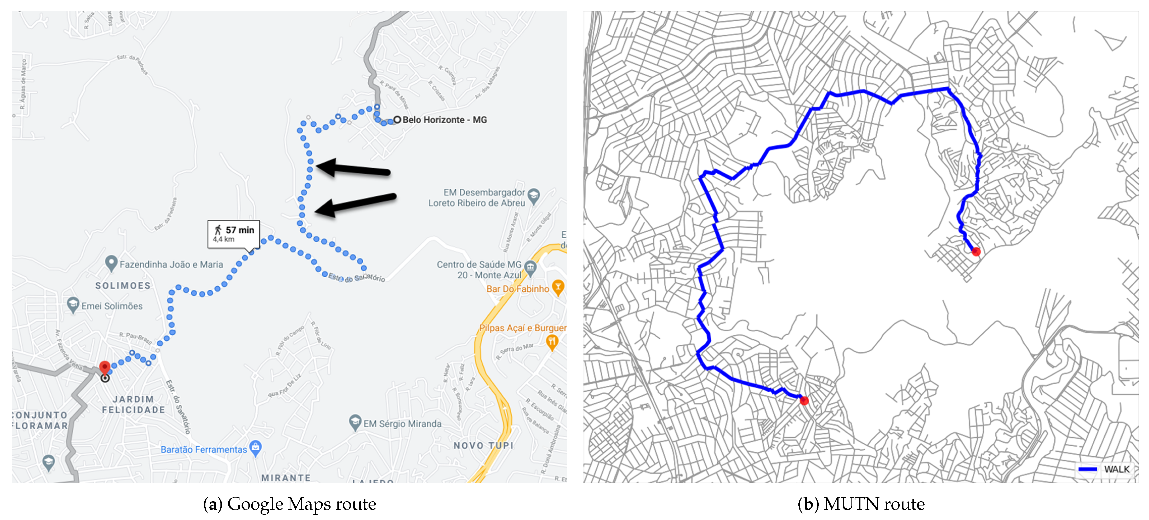
While the routes for DRIVE and WALK had a difference of less than 10% in both time and distance, TRANSIT results obtained higher values, of 17.5% and 19.4% of difference for distance and time, respectively. When investigating some routes with a more significant difference, we observed that, in certain situations, the MUTN network traced longer routes than Google Maps. Figure 8a shows the route in which the most significant difference in relative distance occurred. The Google Maps route uses a path in which there is no apparent connection in the map segments, and returned a route length of 4394 m. Routing on the MUTN network only returns routes by connected segments (Figure 8b). The route length returned by MUTN was 11,183.68 m. Another hypothesis to explain the difference in TRANSIT’s routes may be the transition cost between routes or when entering the collective transportation network that can return different routes from those returned by Google Maps.

The proposed data model proved adequate as a frame of reference to organize the process and to integrate the data in a structure that is suitable for the necessary processing. The final result of MUTN for Belo Horizonte and associated data took up 177 MB of disk space.

7. Conclusions and Future Work

In this work, spatial data integration methods and a data model to store the results were proposed. The spatial data integration method is composed of schema matching steps, data matching, and data fusion. In the schema matching stage, datasets with different schemas and detail levels are made compatible with the proposed data model. In the data matching stage, matching pairs are found in the datasets, with different cardinalities, full (one-to-one), contains and within (one-to-many), and partial (many-to-many). The segments that have no matching candidate are identified and marked as null matches. In the data fusion stage, such null matches can be incorporated into the integrated database, and attributes can be transferred and consolidated. Once the datasets were integrated, information regarding collective transportation and transitions between modes of transport were incorporated, also using data integration methods.

The methods were tested on real-world data for the city of Belo Horizonte. Data from authoritative and crowdsourced datasets were integrated into a multimodal dataset, containing information that allows performing multimodal routing and analysis in the urban environment. The routes created in the process were compared with Google Maps, showing close results. For the routes related to collective transportation that presented a more considerable discrepancy, we identified that differences could be partially explained by limitations in Google Maps, which lead to routes that use apparently disconnected segments. Another hypothesis raised for the differences relates to the cost estimation used in the MUTN model. As there is no precise information on how Google Maps gets its results, a more precise comparison is difficult. Nevertheless, the results obtained can help in several urban analyses, such as mobility (times, costs, mode options), accessibility studies, and transit planning. The method is generic and can be used to integrate various datasets, and the process can be chained to integrate more than two datasets, as shown in the case study.

Limitations identified for our work include (1) the need to establish reference values for thresholds in data integration processes; (2) difficulties in matching features with a large differences as to the level of detail; (3) difficulties in updating the MUTN from changes in the original datasets, requiring the re-execution of the entire data integration process; (4) lack of a user-friendly interface for using the framework. These limitations also indicate directions for future research. The data integration process needs further study to determine thresholds or tolerance values in the calculation of similarity metrics. However, the establishment of an optimal value that maximizes correct matches, minimizes or prevents incorrect matches, and balance performance with results is not simple and depends on the quality (positional accuracy) and other characteristics of the input data, such as the road pattern [96]. For example, data of streets organized in gridiron with high positional accuracy can have a lower threshold for angle similarity than data with lower positional accuracy or with streets distributed in a loops and lollipops street pattern. The immediate approach would be to find the values empirically [34]. An approach using machine learning techniques to determine the optimal values for the thresholds should be investigated. Another future research need is to find ways to avoid the re-execution of the data integration process when part of the original data is modified. For OSM data, it may be possible to leverage the edit history metadata and to incorporate only the changes into the integrated data view. A current difficulty in using the framework is the lack of a more user-friendly and intuitive interface. One possibility is the implementation of a plugin to allow access and use of the framework from open source GIS tools such as QGIS (https://www.qgis.org/ (accesssed on 7 August 2020)).