
Crime Risk Stations: Examining Spatiotemporal Influence of Urban Features through Distance-Aware Risk Signal Functions


Abstract
:1. Introduction
- How do the spatial influences of urban features change within a spatial extent?
- How does a spatial influence operate within a spatial extent?
- Based on a crime-specific spatiotemporal approach:
- How does the spatial influence of an urban feature vary across the sub-regions of a city based on the time of day and the day of the week?
- How does the spatial influence of an urban feature vary across crime types?
- How does a crime-specific spatiotemporal influence interact with the characteristics of the social environment?
1.1. Spatial Influence
1.2. Characteristics of Spatial Extent
1.3. Spatial Influence in an Environmental Backcloth
1.4. This Study
2. Materials and Methods
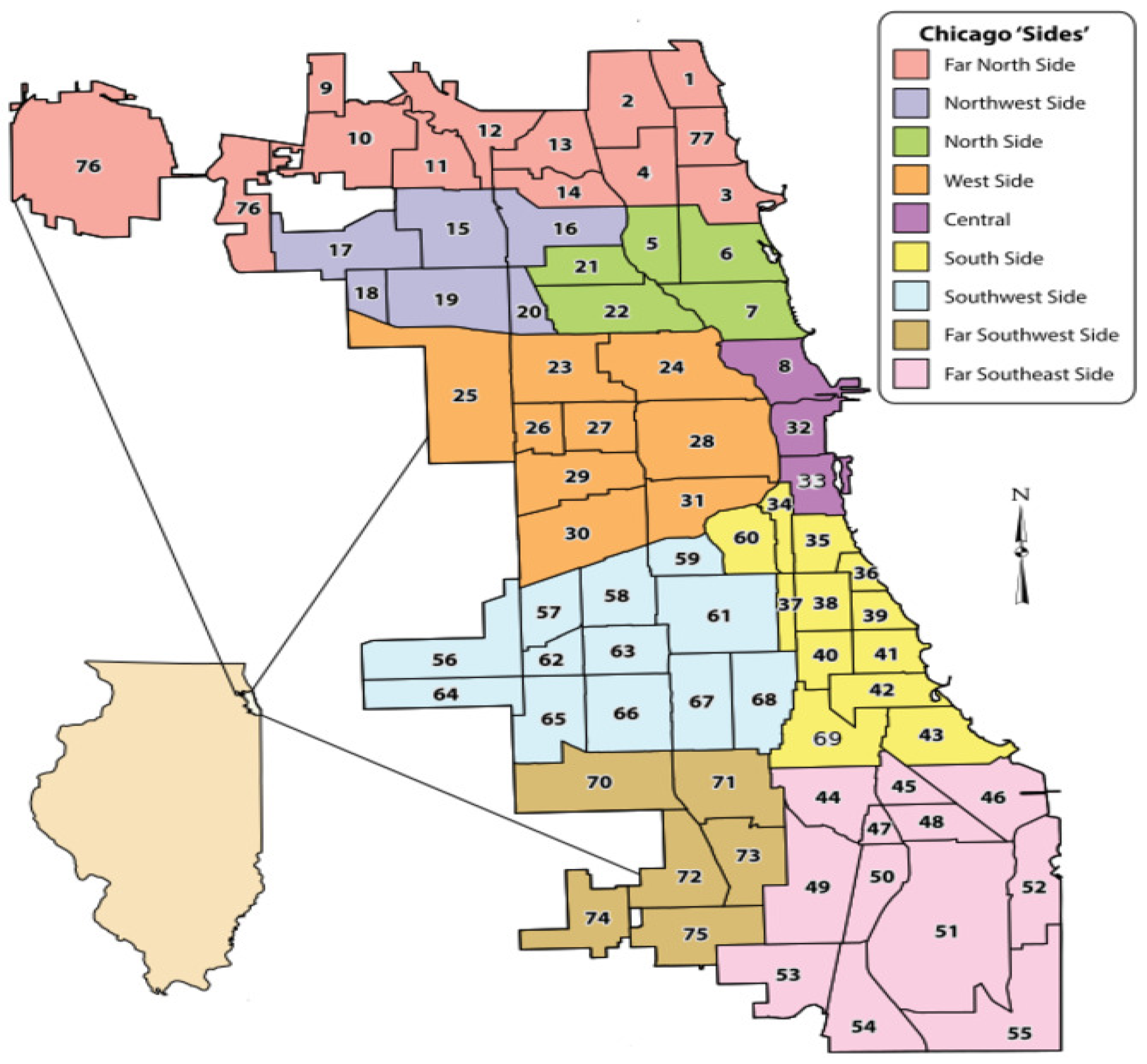
2.1. Study Setting
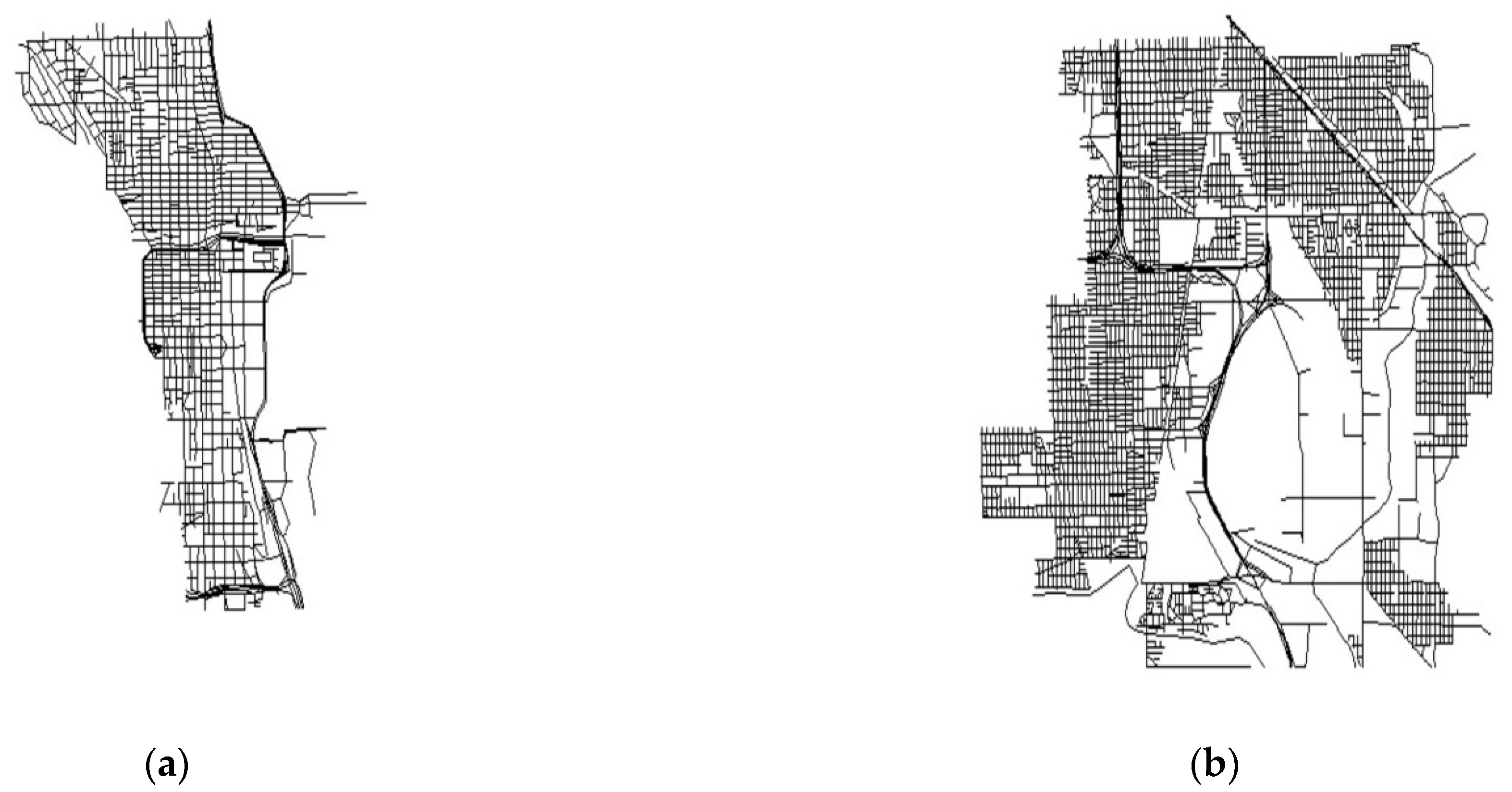
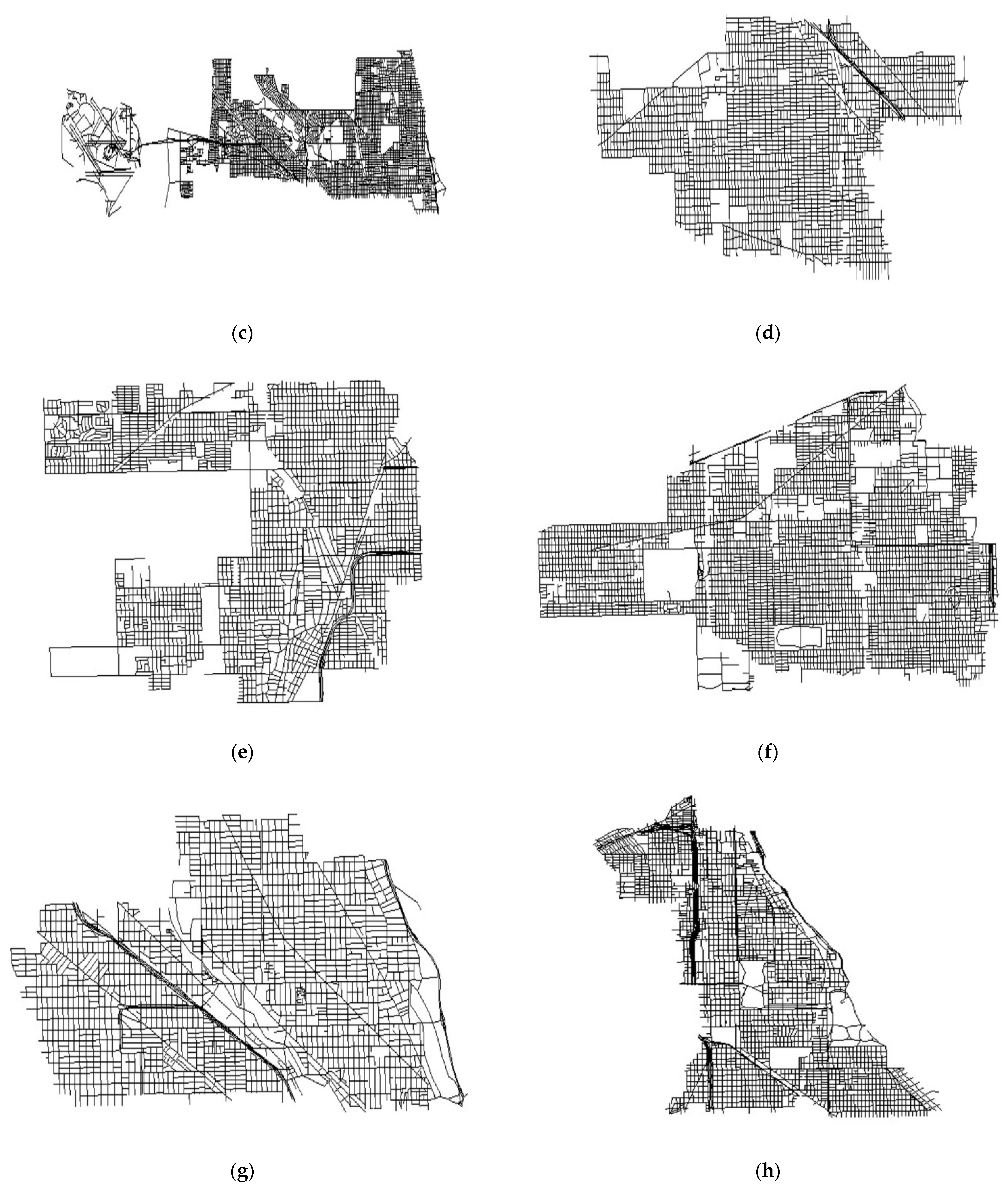
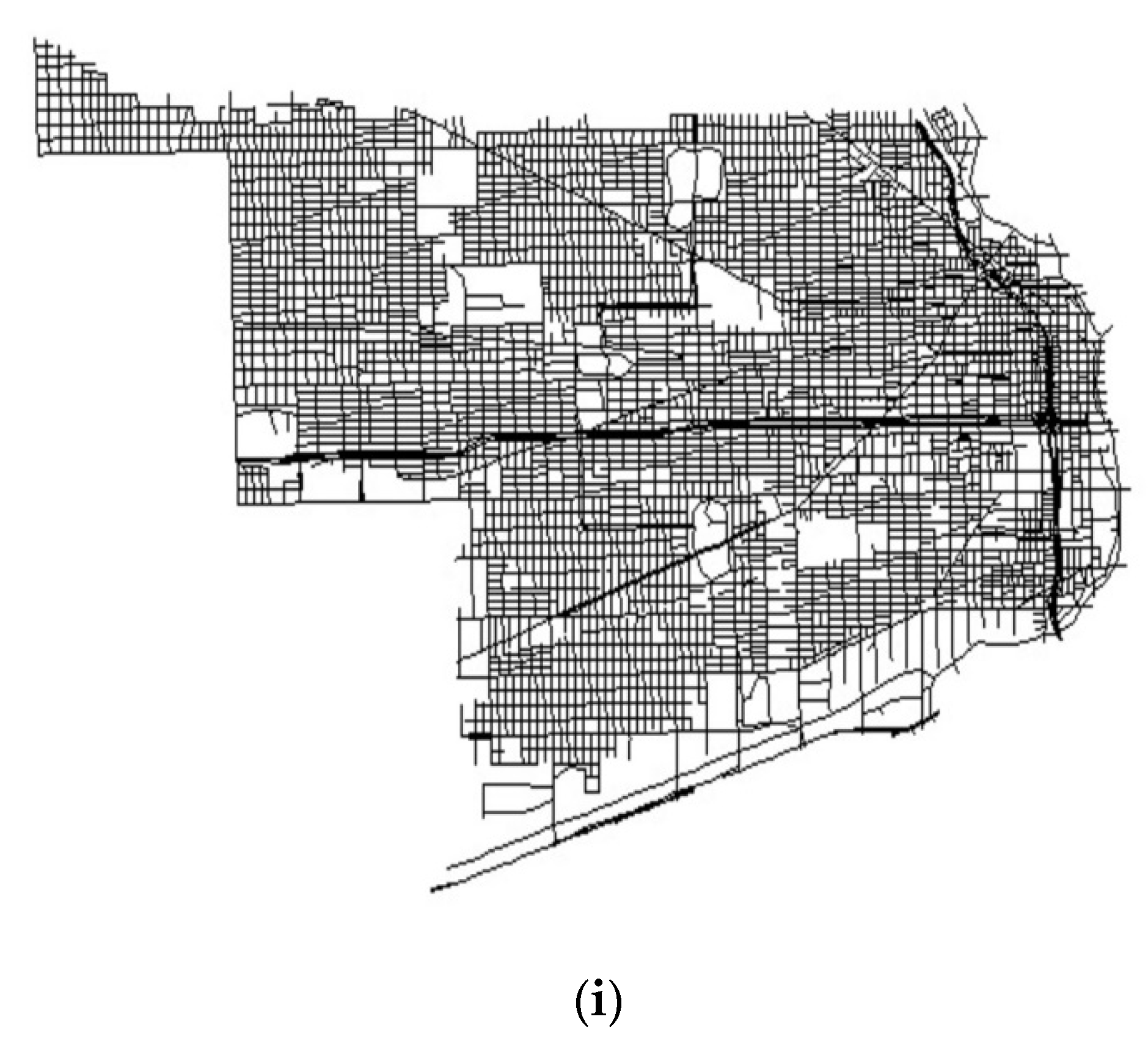
2.2. Creating Street Networks for the Sides of Chicago
2.3. Crime Dataset
2.4. Urban Features
2.5. Concentrated Disadvantage (CD)
2.6. Network K Function
2.7. Risk Signal Functions, RSIS and RSSS
2.8. Analytical Procedure
3. Results
3.1. Network K Analysis
3.2. Spatiotemporal Influence Analysis
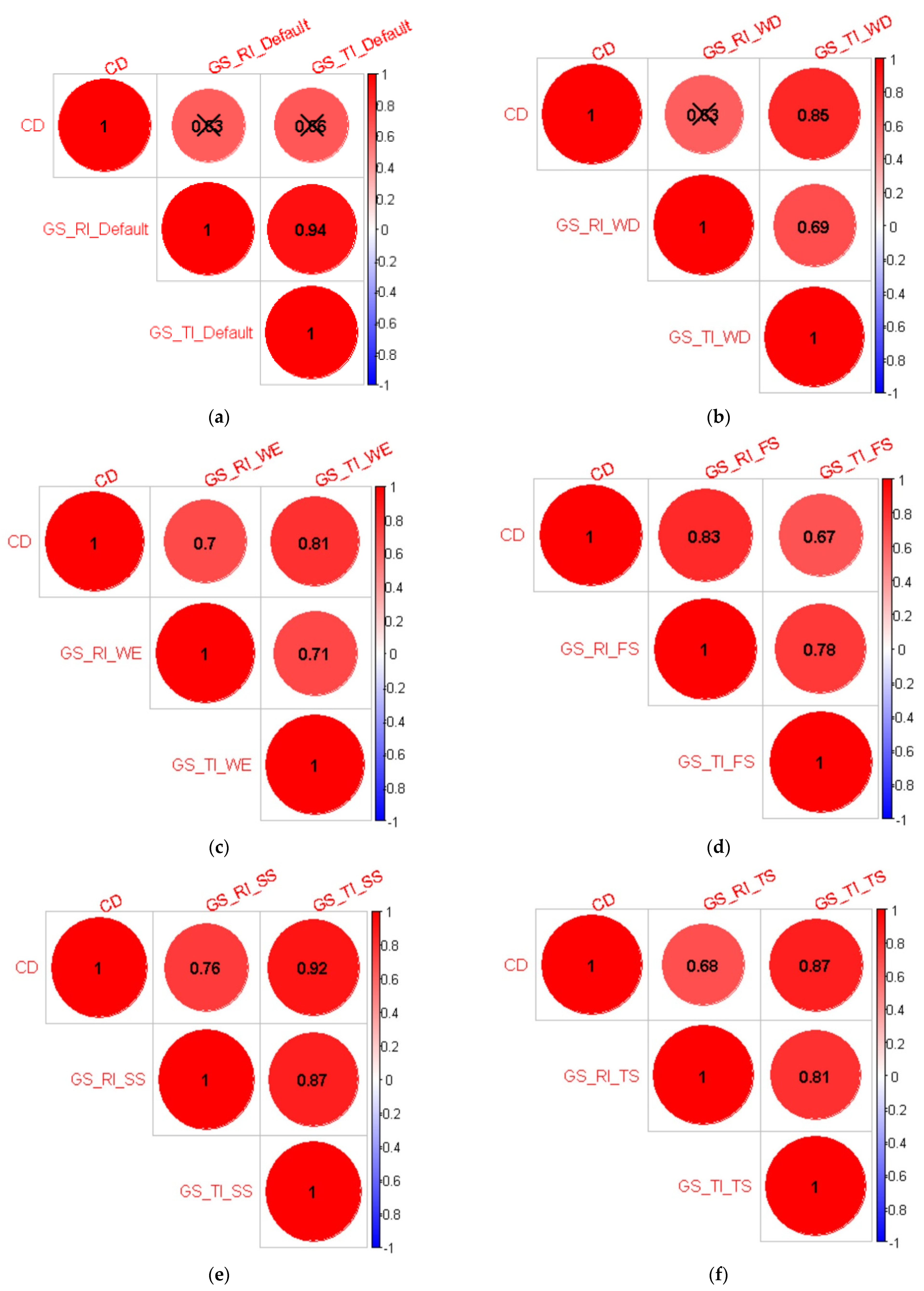
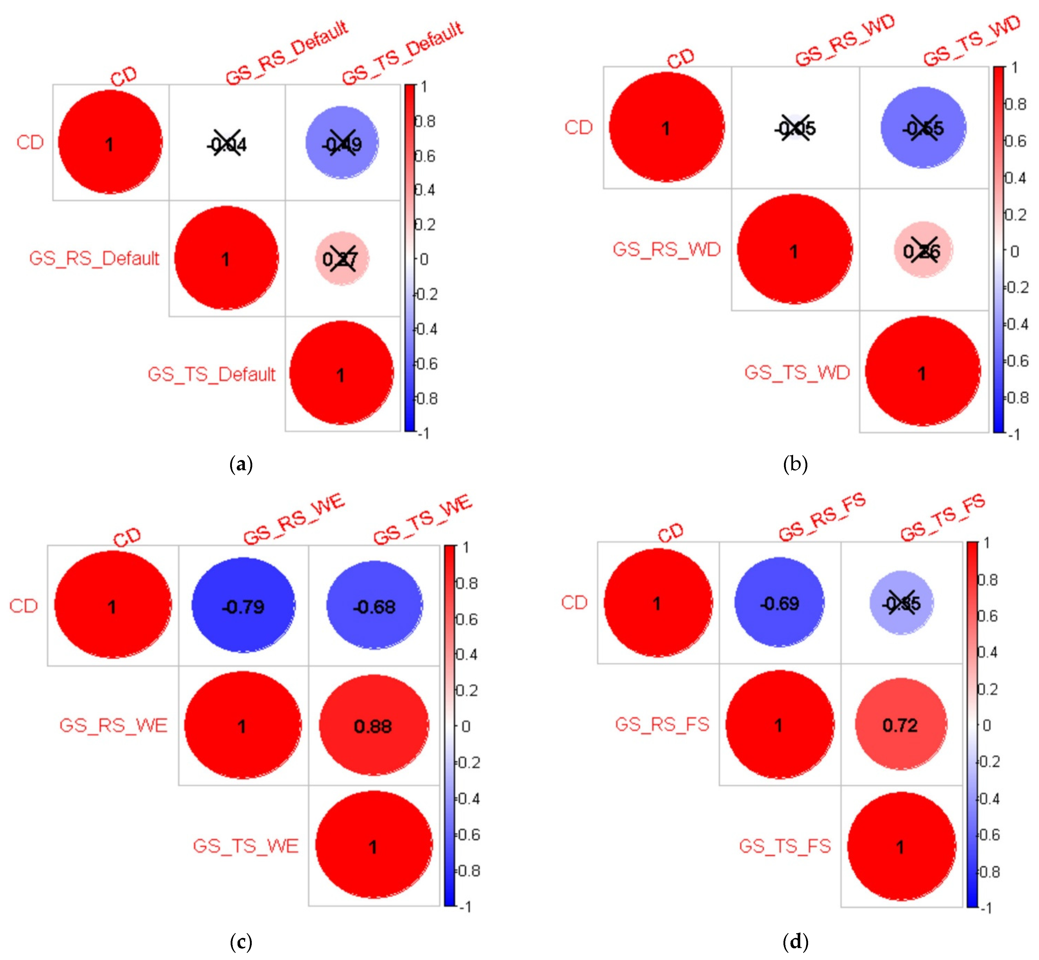
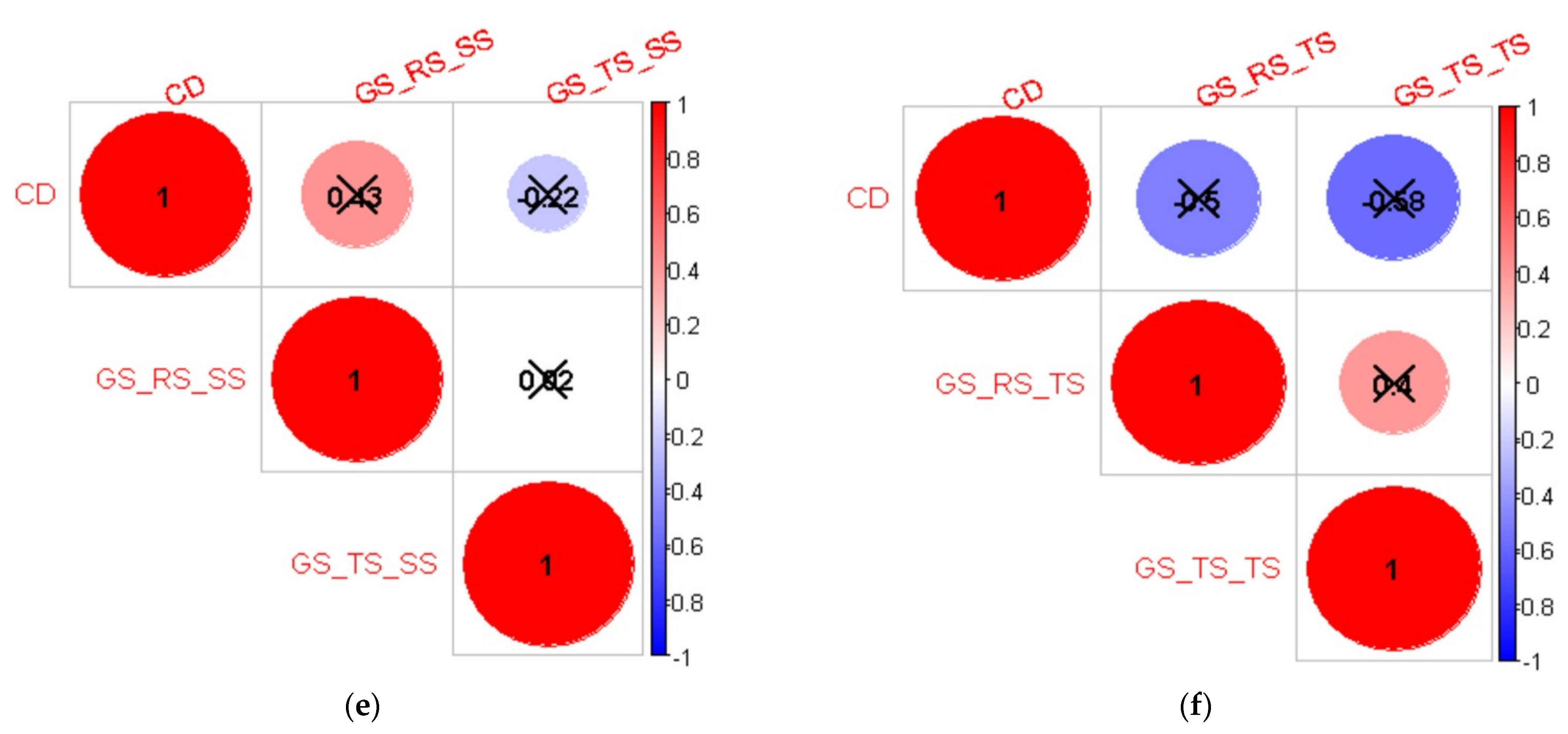
3.3. Correlation Analysis with Concentrated Disadvantage (CD)
4. Discussion
5. Conclusions
5.1. Research Implications
5.2. Practical Implications
5.3. Limitations
5.4. Future Research
Author Contributions
Funding
Data Availability Statement
Acknowledgments
Conflicts of Interest
Appendix A

| Robbery | Theft | ||||||||||||
|---|---|---|---|---|---|---|---|---|---|---|---|---|---|
| Sides | Default | WD | WE | FS | SS | TS | Default | WD | WE | FS | SS | TS | |
| Bus Stop | Center | ✓ | ✓ | ✓ | ✓ | ✓ | ✓ | ✓ | ✓ | ✓ | ✓ | ✓ | ✓ |
| Far North | ✓ | ✓ | ✓ | ✓ | ✓ | ✓ | ✓ | ✓ | ✓ | ✓ | ✓ | ✓ | |
| Far South East | ✓ | ✓ | ✓ | ✓ | ✓ | ✓ | ✓ | ✓ | ✓ | ✓ | ✓ | ✓ | |
| Far South West | ✓ | ✓ | ✓ | ✓ | ✓ | ✓ | ✓ | ✓ | ✓ | ✓ | ✓ | ✓ | |
| North | ✓ | ✓ | ✓ | ✓ | ✓ | ✓ | ✓ | ✓ | ✓ | ✓ | ✓ | ✓ | |
| North West | ✓ | ✓ | ✓ | ✓ | ✓ | ✓ | ✓ | ✓ | ✓ | ✓ | ✓ | ✓ | |
| South | ✓ | ✓ | ✓ | ✓ | ✓ | ✓ | ✓ | ✓ | ✓ | ✓ | ✓ | ✓ | |
| South West | ✓ | ✓ | ✓ | ✓ | ✓ | ✓ | ✓ | ✓ | ✓ | ✓ | ✓ | ✓ | |
| West | ✓ | ✓ | ✓ | ✓ | ✓ | ✓ | ✓ | ✓ | ✓ | ✓ | ✓ | ✓ | |
| Fast Food Restaurant | Center | ✓ | ✓ | ✓ | ✓ | ✓ | ✓ | ✓ | ✓ | ✓ | ✓ | ✓ | ✓ |
| Far North | ✓ | ✓ | ✓ | ✓ | ✓ | ✓ | ✓ | ✓ | ✓ | ✓ | ✓ | ✓ | |
| Far South East | ✓ | ✓ | ✓ | ✓ | ✓ | ✓ | ✓ | ✓ | ✓ | ✓ | ✓ | ✓ | |
| Far South West | ✓ | ✓ | ✓ | ✓ | ✓ | ✓ | ✓ | ✓ | ✓ | ✓ | ✓ | ✓ | |
| North | ✓ | ✓ | ✓ | ✓ | ✓ | ✓ | ✓ | ✓ | ✓ | ✓ | ✓ | ✓ | |
| North West | ✓ | ✓ | ✓ | ✓ | ✓ | ✓ | ✓ | ✓ | ✓ | ✓ | ✓ | ✓ | |
| South | ✓ | ✓ | ✓ | ✓ | ✓ | ✓ | ✓ | ✓ | ✓ | ✓ | ✓ | ✓ | |
| South West | ✓ | ✓ | ✓ | ✓ | ✓ | ✓ | ✓ | ✓ | ✓ | ✓ | ✓ | ✓ | |
| West | ✓ | ✓ | ✓ | ✓ | ✓ | ✓ | ✓ | ✓ | ✓ | ✓ | ✓ | ✓ | |
| Gas Station | Center | ✕ | ✓ | ✕ | ✕ | ✕ | ✕ | ✕ | ✕ | ✕ | ✕ | ✕ | ✕ |
| Far North | ✓ | ✓ | ✓ | ✓ | ✕ | ✕ | ✓ | ✓ | ✓ | ✓ | ✓ | ✓ | |
| Far South East | ✓ | ✓ | ✓ | ✓ | ✓ | ✓ | ✓ | ✓ | ✓ | ✓ | ✓ | ✓ | |
| Far South West | ✓ | ✓ | ✓ | ✓ | ✓ | ✓ | ✓ | ✓ | ✓ | ✓ | ✓ | ✓ | |
| North | ✓ | ✕ | ✕ | ✕ | ✕ | ✕ | ✓ | ✕ | ✓ | ✓ | ✕ | ✕ | |
| North West | ✓ | ✓ | ✓ | ✓ | ✓ | ✓ | ✓ | ✓ | ✓ | ✓ | ✓ | ✓ | |
| South | ✓ | ✓ | ✓ | ✓ | ✓ | ✓ | ✓ | ✓ | ✓ | ✓ | ✓ | ✓ | |
| South West | ✓ | ✓ | ✓ | ✓ | ✓ | ✓ | ✓ | ✓ | ✓ | ✓ | ✓ | ✓ | |
| West | ✓ | ✓ | ✓ | ✓ | ✓ | ✓ | ✓ | ✓ | ✓ | ✓ | ✓ | ✓ | |
| Grocery Store | Center | ✓ | ✓ | ✓ | ✓ | ✓ | ✓ | ✓ | ✓ | ✓ | ✓ | ✓ | ✓ |
| Far North | ✓ | ✓ | ✓ | ✓ | ✓ | ✓ | ✓ | ✓ | ✓ | ✓ | ✓ | ✓ | |
| Far South East | ✓ | ✓ | ✓ | ✓ | ✓ | ✓ | ✓ | ✓ | ✓ | ✓ | ✓ | ✓ | |
| Far South West | ✓ | ✓ | ✓ | ✓ | ✓ | ✓ | ✓ | ✓ | ✓ | ✓ | ✓ | ✓ | |
| North | ✓ | ✓ | ✓ | ✓ | ✓ | ✓ | ✓ | ✓ | ✓ | ✓ | ✓ | ✓ | |
| North West | ✓ | ✓ | ✓ | ✕ | ✓ | ✓ | ✓ | ✓ | ✓ | ✓ | ✓ | ✓ | |
| South | ✓ | ✓ | ✓ | ✓ | ✓ | ✓ | ✓ | ✓ | ✓ | ✓ | ✓ | ✓ | |
| South West | ✓ | ✓ | ✓ | ✓ | ✓ | ✓ | ✓ | ✓ | ✓ | ✓ | ✓ | ✓ | |
| West | ✓ | ✓ | ✓ | ✓ | ✓ | ✓ | ✓ | ✓ | ✓ | ✓ | ✓ | ✓ | |
| Pub/Taverns | Center | ✓ | ✓ | ✓ | ✓ | ✓ | ✓ | ✓ | ✓ | ✓ | ✓ | ✓ | ✓ |
| Far North | ✓ | ✓ | ✓ | ✓ | ✓ | ✓ | ✓ | ✓ | ✓ | ✓ | ✓ | ✓ | |
| Far South East | ✓ | ✓ | ✓ | ✓ | ✓ | ✓ | ✓ | ✓ | ✓ | ✓ | ✓ | ✓ | |
| Far South West | ✓ | ✕ | ✓ | ✓ | ✕ | ✓ | ✓ | ✓ | ✓ | ✓ | ✓ | ✓ | |
| North | ✓ | ✓ | ✓ | ✓ | ✓ | ✓ | ✓ | ✓ | ✓ | ✓ | ✓ | ✓ | |
| North West | ✓ | ✓ | ✓ | ✓ | ✓ | ✓ | ✓ | ✓ | ✓ | ✓ | ✓ | ✓ | |
| South | ✓ | ✓ | ✕ | ✕ | ✓ | ✓ | ✓ | ✓ | ✓ | ✓ | ✓ | ✓ | |
| South West | ✓ | ✓ | ✕ | ✕ | ✓ | ✕ | ✓ | ✓ | ✓ | ✓ | ✓ | ✓ | |
| West | ✓ | ✕ | ✓ | ✓ | ✕ | ✓ | ✓ | ✓ | ✓ | ✓ | ✓ | ✓ | |
Appendix B
| Robbery | Theft | ||||||||||||
|---|---|---|---|---|---|---|---|---|---|---|---|---|---|
| Sides | Default | WD | WE | FS | SS | TS | Default | WD | WE | FS | SS | TS | |
| Bus Stop | Center | 1.74 | 1.81 | 1.73 | 1.80 | 1.94 | 1.69 | 1.62 | 1.63 | 1.58 | 1.56 | 1.62 | 1.62 |
| Far North | 2.21 | 2.43 | 1.83 | 2.45 | 2.07 | 2.12 | 1.77 | 1.76 | 1.78 | 1.69 | 1.92 | 1.64 | |
| Far South East | 2.15 | 2.12 | 2.20 | 2.06 | 2.30 | 2.10 | 2.09 | 2.12 | 2.05 | 1.59 | 2.28 | 2.09 | |
| Far South West | 2.07 | 2.10 | 2.01 | 2.03 | 1.99 | 16.56 | 1.79 | 1.75 | 1.93 | 1.51 | 1.94 | 13.00 | |
| North | 1.58 | 1.52 | 1.65 | 1.71 | 1.51 | 1.48 | 1.56 | 1.54 | 1.59 | 1.52 | 1.58 | 1.56 | |
| North West | 1.43 | 1.42 | 1.46 | 1.40 | 1.84 | 1.38 | 1.56 | 1.57 | 1.54 | 1.41 | 1.74 | 1.48 | |
| South | 1.38 | 1.35 | 1.37 | 1.37 | 1.38 | 1.34 | 1.39 | 1.39 | 1.39 | 1.30 | 1.43 | 1.38 | |
| South West | 1.42 | 1.42 | 1.48 | 1.38 | 1.49 | 1.49 | 1.51 | 1.49 | 1.56 | 1.25 | 1.62 | 1.51 | |
| West | 1.40 | 1.45 | 1.32 | 1.36 | 1.40 | 1.42 | 1.29 | 1.31 | 1.26 | 1.21 | 1.36 | 1.26 | |
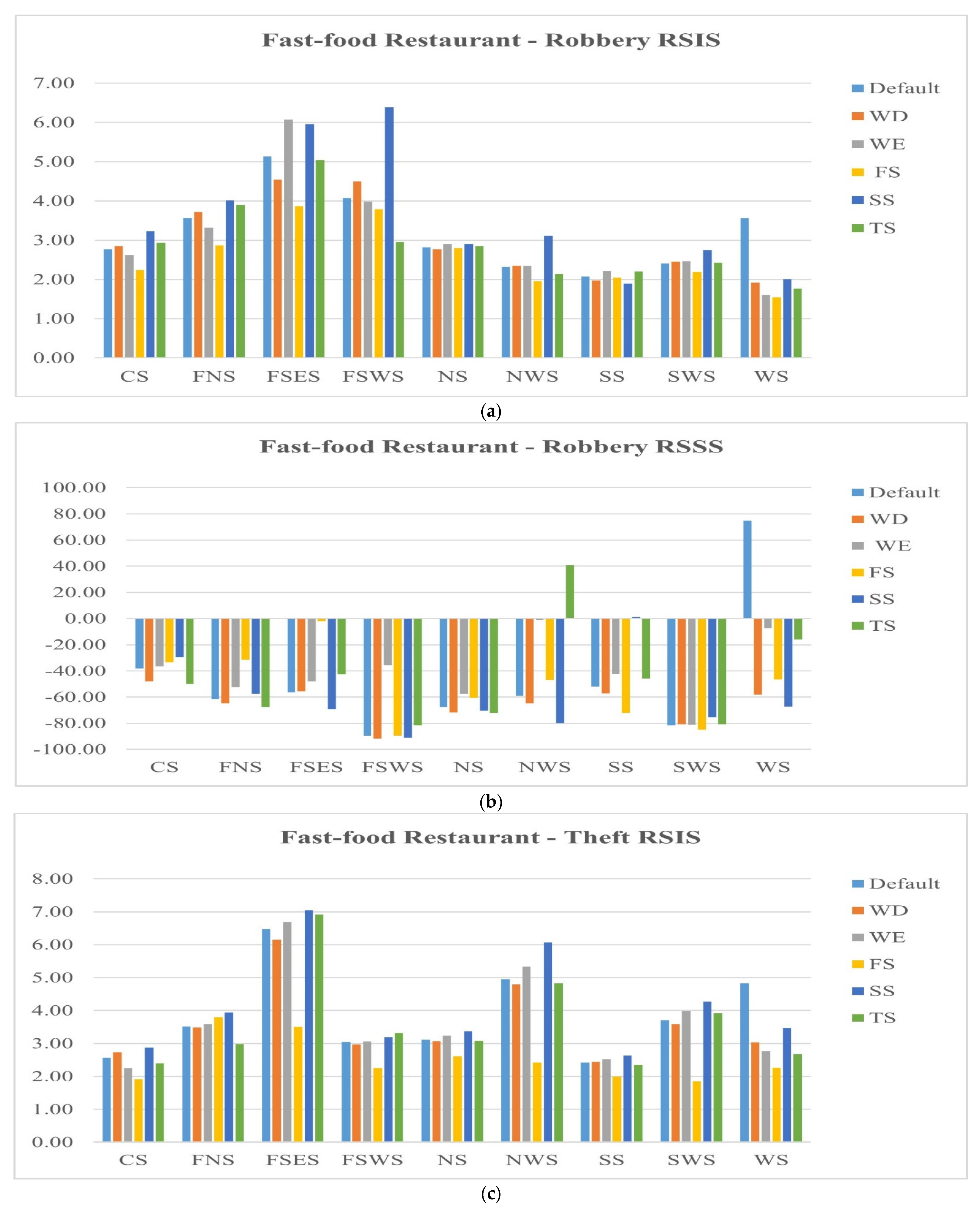
| Fast Food Restaurant | Center | 2.77 | 2.85 | 2.62 | 2.24 | 3.23 | 2.94 | 2.56 | 2.73 | 2.26 | 1.91 | 2.87 | 2.39 |
| Far North | 3.56 | 3.72 | 3.32 | 2.87 | 4.01 | 3.89 | 3.52 | 3.48 | 3.59 | 3.80 | 3.94 | 2.98 | |
| Far South East | 5.13 | 4.55 | 6.08 | 3.87 | 5.96 | 5.04 | 6.48 | 6.15 | 6.69 | 3.50 | 7.05 | 6.92 | |
| Far South West | 4.07 | 4.49 | 3.99 | 3.79 | 6.38 | 2.96 | 3.05 | 2.97 | 3.06 | 2.25 | 3.19 | 3.31 | |
| North | 2.82 | 2.77 | 2.91 | 2.80 | 2.91 | 2.85 | 3.11 | 3.07 | 3.23 | 2.61 | 3.37 | 3.07 | |
| North West | 2.32 | 2.34 | 2.35 | 1.95 | 3.11 | 2.15 | 4.95 | 4.80 | 5.33 | 2.41 | 6.07 | 4.83 | |
| South | 2.08 | 1.97 | 2.22 | 2.04 | 1.90 | 2.20 | 2.42 | 2.44 | 2.52 | 1.99 | 2.63 | 2.36 | |
| South West | 2.41 | 2.45 | 2.46 | 2.19 | 2.75 | 2.43 | 3.71 | 3.59 | 3.98 | 1.84 | 4.27 | 3.92 | |
| West | 3.56 | 1.92 | 1.60 | 1.55 | 2.00 | 1.77 | 4.83 | 3.04 | 2.77 | 2.27 | 3.47 | 2.68 | |
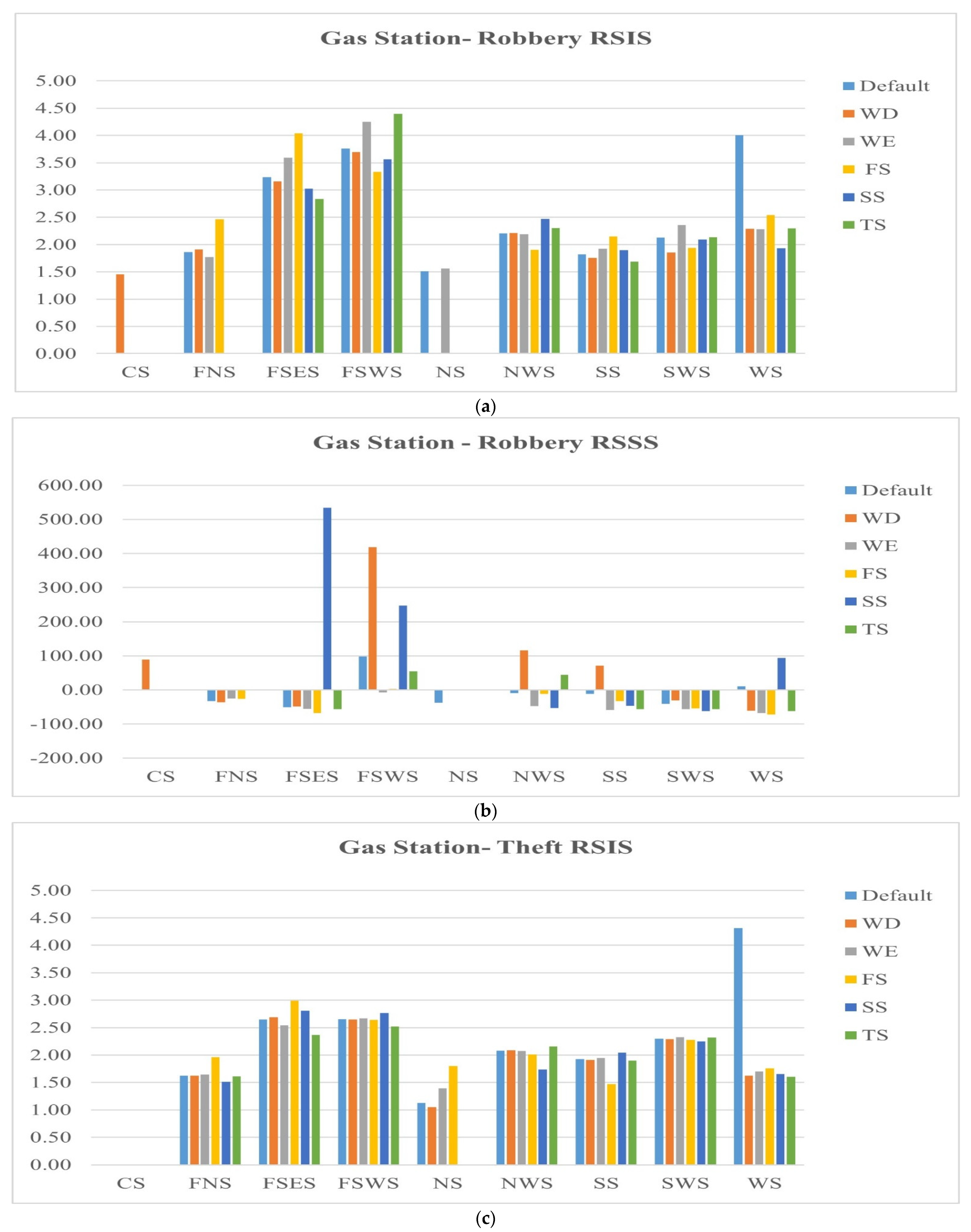
| Gas Station | Center | 0.00 | 1.46 | 0.00 | 0.00 | 0.00 | 0.00 | 0.00 | 0.00 | 0.00 | 0.00 | 0.00 | 0.00 |
| Far North | 1.86 | 1.91 | 1.77 | 2.46 | 0.00 | 0.00 | 1.63 | 1.62 | 1.65 | 1.96 | 1.51 | 1.61 | |
| Far South East | 3.23 | 3.16 | 3.59 | 4.04 | 3.03 | 2.83 | 2.65 | 2.69 | 2.54 | 2.99 | 2.81 | 2.37 | |
| Far South West | 3.76 | 3.70 | 4.25 | 3.33 | 3.56 | 4.40 | 2.66 | 2.65 | 2.67 | 2.64 | 2.76 | 2.52 | |
| North | 1.51 | 0.00 | 0.00 | 0.00 | 0.00 | 0.00 | 1.13 | 1.05 | 1.39 | 1.80 | 0.00 | 0.00 | |
| North West | 2.21 | 2.21 | 2.19 | 1.90 | 2.47 | 2.30 | 2.08 | 2.09 | 2.07 | 2.01 | 1.73 | 2.16 | |
| South | 1.82 | 1.76 | 1.92 | 2.15 | 1.89 | 1.69 | 1.92 | 1.91 | 1.95 | 1.47 | 2.04 | 1.90 | |
| South West | 2.12 | 1.85 | 2.36 | 1.94 | 2.09 | 2.14 | 2.30 | 2.29 | 2.33 | 2.28 | 2.25 | 2.32 | |
| West | 4.01 | 2.29 | 2.28 | 2.54 | 1.93 | 2.30 | 4.32 | 1.62 | 1.71 | 1.76 | 1.65 | 1.60 | |
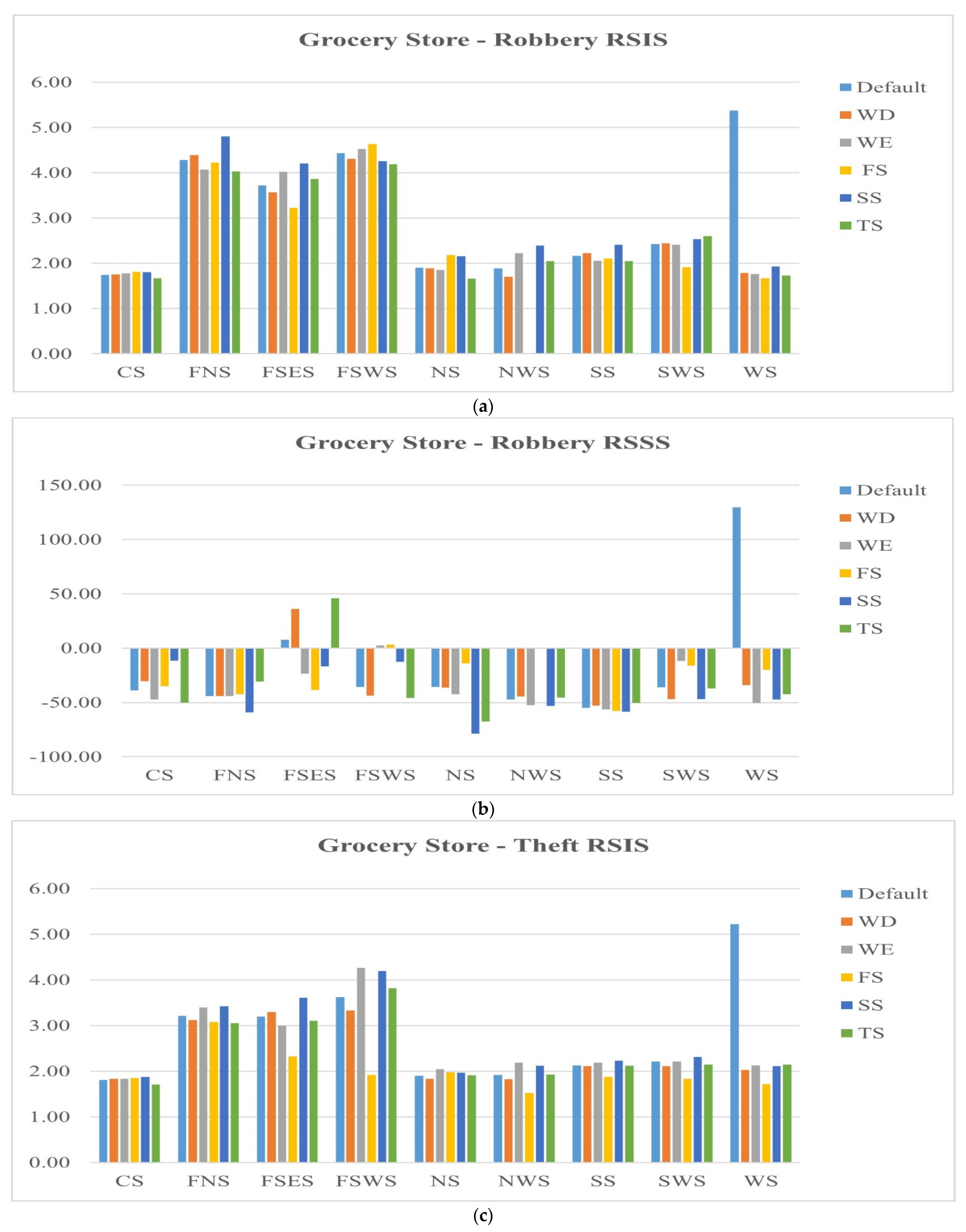
| Grocery Store | Center | 1.74 | 1.75 | 0.00 | 1.81 | 1.80 | 1.67 | 1.81 | 1.84 | 1.84 | 1.85 | 1.88 | 1.71 |
| Far North | 4.28 | 4.39 | 4.07 | 4.22 | 4.80 | 4.03 | 3.22 | 3.12 | 3.40 | 3.08 | 3.43 | 3.05 | |
| Far South East | 3.72 | 3.57 | 4.03 | 3.22 | 4.21 | 3.87 | 3.19 | 3.29 | 2.99 | 2.32 | 3.61 | 3.11 | |
| Far South West | 4.43 | 4.31 | 4.53 | 4.64 | 4.26 | 4.19 | 3.62 | 3.33 | 4.27 | 1.92 | 4.19 | 3.82 | |
| North | 1.90 | 0.00 | 0.00 | 2.18 | 2.16 | 1.66 | 1.90 | 1.83 | 2.05 | 1.98 | 1.97 | 1.91 | |
| North West | 1.89 | 1.71 | 2.22 | 0.00 | 2.39 | 2.05 | 1.92 | 1.83 | 2.19 | 1.52 | 2.12 | 1.93 | |
| South | 2.17 | 2.22 | 2.05 | 2.11 | 2.41 | 2.05 | 2.13 | 2.11 | 2.19 | 1.88 | 2.23 | 2.12 | |
| South West | 2.42 | 2.44 | 2.41 | 1.91 | 2.54 | 2.60 | 2.21 | 2.11 | 2.21 | 1.84 | 2.31 | 2.15 | |
| West | 5.37 | 1.79 | 1.77 | 1.67 | 1.93 | 1.73 | 5.22 | 2.03 | 2.13 | 1.71 | 2.11 | 2.15 | |
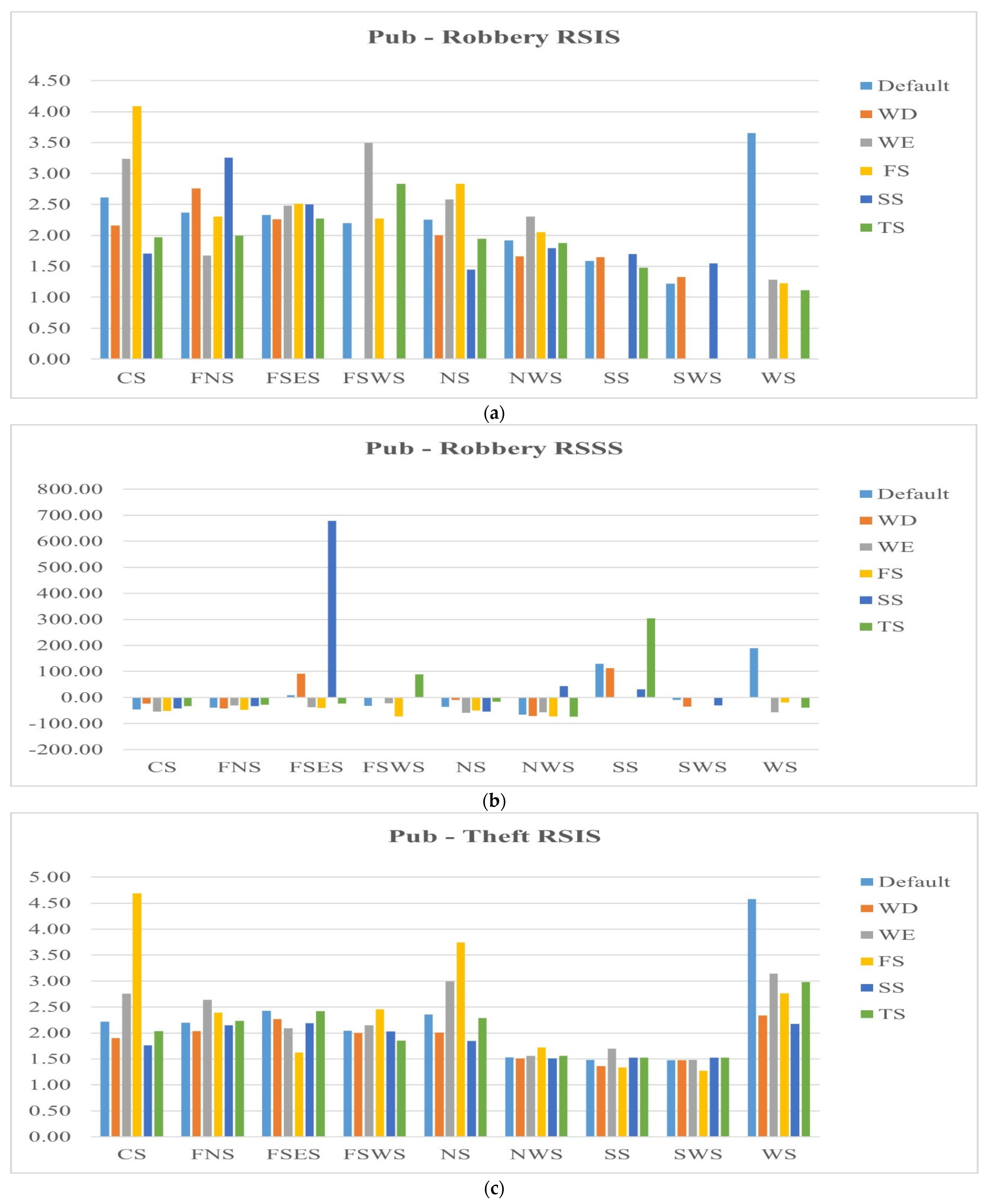
| Pub/Taverns | Center | 2.61 | 2.16 | 3.23 | 4.09 | 1.71 | 1.97 | 2.22 | 1.90 | 2.76 | 4.69 | 1.76 | 2.03 |
| Far North | 2.37 | 2.76 | 1.67 | 2.30 | 3.26 | 2.00 | 2.20 | 2.04 | 2.63 | 2.39 | 2.15 | 2.23 | |
| Far South East | 2.33 | 2.26 | 2.48 | 2.51 | 2.50 | 2.27 | 2.43 | 2.26 | 2.09 | 1.62 | 2.19 | 2.42 | |
| Far South West | 2.20 | 0.00 | 3.50 | 2.27 | 0.00 | 2.83 | 2.04 | 2.00 | 2.15 | 2.45 | 2.03 | 1.86 | |
| North | 2.25 | 2.00 | 2.58 | 2.83 | 1.44 | 1.94 | 2.36 | 2.00 | 2.99 | 3.75 | 1.84 | 2.29 | |
| North West | 1.92 | 1.66 | 2.30 | 2.05 | 1.79 | 1.87 | 1.53 | 1.51 | 1.56 | 1.72 | 1.51 | 1.56 | |
| South | 1.58 | 1.65 | 0.00 | 0.00 | 1.70 | 1.48 | 1.48 | 1.36 | 1.70 | 1.34 | 1.53 | 1.52 | |
| South West | 1.22 | 1.33 | 0.00 | 0.00 | 1.55 | 0.00 | 1.47 | 1.47 | 1.48 | 1.27 | 1.52 | 1.52 | |
| West | 3.66 | 0.00 | 1.28 | 1.23 | 0.00 | 1.11 | 4.58 | 2.34 | 3.14 | 2.76 | 2.18 | 2.98 | |
| Robbery | Theft | ||||||||||||
|---|---|---|---|---|---|---|---|---|---|---|---|---|---|
| Sides | Default | WD | WE | FS | SS | TS | Default | WD | WE | FS | SS | TS | |
| Bus Stop | Center | −2.62 | −1.22 | 3.41 | −1.07 | −20.70 | 2.41 | −30.84 | −30.47 | −32.21 | 33.36 | −32.39 | −34.54 |
| Far North | −4.66 | −4.44 | −5.26 | −22.41 | −12.34 | 20.02 | −10.14 | −6.55 | −16.79 | −26.61 | −7.34 | −4.87 | |
| Far South East | −0.46 | 7.13 | −67.90 | 1.20 | 1.93 | −3.09 | 20.17 | 27.04 | 7.40 | 38.63 | 18.16 | 18.05 | |
| Far South West | 16.73 | 13.16 | −2.97 | 6.22 | 5.05 | 128.43 | 76.50 | 96.62 | 89.63 | 316.88 | 91.26 | 113.40 | |
| North | 11.19 | 20.36 | −3.95 | −18.50 | 64.16 | 53.11 | 54.39 | 49.89 | 42.75 | 23.82 | 41.99 | 70.11 | |
| North West | 84.68 | 74.59 | 109.42 | 51.56 | 6.97 | 66.47 | 53.25 | 54.50 | 51.28 | 53.17 | 70.69 | 46.34 | |
| South | 20.46 | 33.65 | 5.01 | 7.55 | 10.43 | 26.56 | 90.14 | 81.51 | 110.47 | 69.86 | 102.87 | 85.03 | |
| South West | 2.64 | 2.33 | 14.15 | −32.45 | 27.52 | 12.37 | 76.78 | 79.00 | 53.71 | 114.18 | 59.62 | 48.66 | |
| West | 9.24 | 5.47 | 16.69 | 15.41 | 12.57 | 3.71 | 36.81 | 37.29 | 36.17 | 47.36 | 43.92 | 25.46 | |
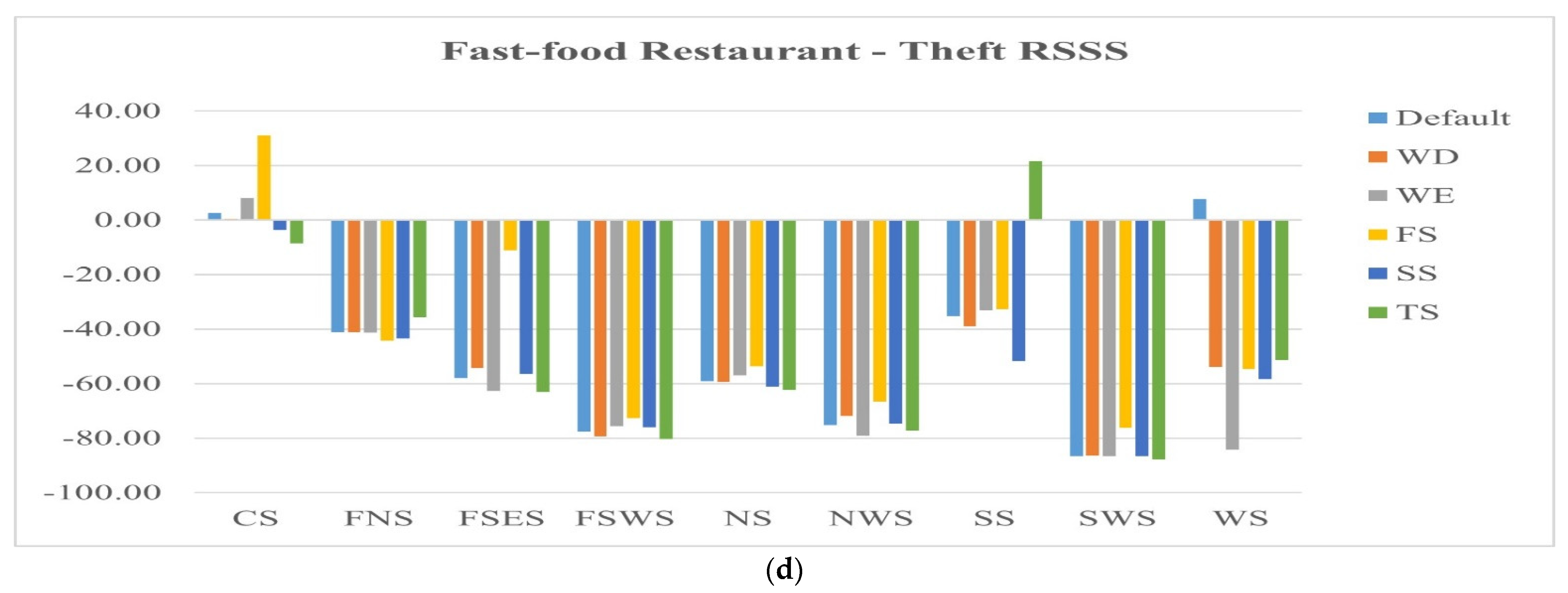
| Fast Food Restaurant | Center | −38.22 | −48.14 | −36.47 | −33.36 | −29.65 | −50.03 | 2.49 | 0.36 | 7.98 | 31.00 | −3.79 | −8.63 |
| Far North | −61.38 | −64.72 | −52.40 | −31.48 | −57.54 | −67.63 | −41.16 | −41.23 | −41.31 | −44.27 | −43.51 | −35.58 | |
| Far South East | −56.32 | −55.54 | −48.06 | −2.09 | −69.18 | −42.66 | −58.00 | −54.32 | −62.67 | −11.16 | −56.44 | −63.04 | |
| Far South West | −89.52 | −91.61 | −35.55 | −89.42 | −91.24 | −81.75 | −77.55 | −79.34 | −75.71 | −72.70 | −76.12 | −80.33 | |
| North | −67.75 | −71.90 | −57.39 | −60.69 | −70.45 | −72.05 | −59.12 | −59.32 | −56.99 | −53.63 | −61.06 | −62.41 | |
| North West | −59.02 | −64.90 | −0.95 | −46.89 | −79.89 | 40.81 | −75.37 | −71.98 | −79.16 | −66.64 | −74.75 | −77.33 | |
| South | −51.79 | −57.37 | −42.05 | −72.04 | 1.23 | −45.67 | −35.22 | −39.02 | −33.20 | −32.70 | −51.69 | 21.65 | |
| South West | −81.63 | −80.83 | −80.97 | −85.00 | −75.58 | −80.77 | −86.57 | −86.52 | −86.71 | −76.33 | −86.68 | −87.87 | |
| West | 74.57 | −58.19 | −7.47 | −46.53 | −67.34 | −16.09 | 7.60 | −53.87 | −84.38 | −54.67 | −58.38 | −51.37 | |
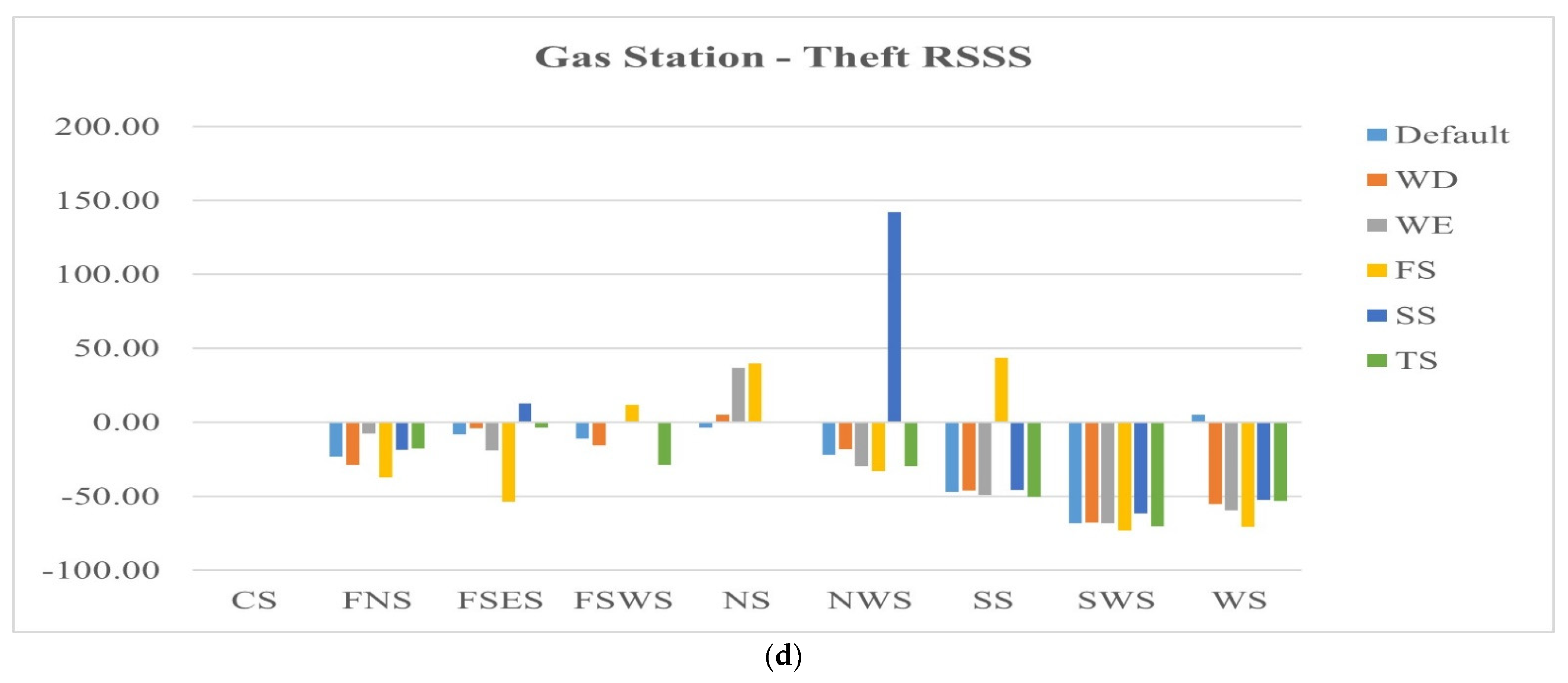
| Gas Station | Center | 0.00 | 89.45 | 0.00 | 0.00 | 0.00 | 0.00 | 0.00 | 0.00 | 0.00 | 0.00 | 0.00 | 0.00 |
| Far North | −33.12 | −36.37 | −25.50 | −26.68 | 0.00 | 0.00 | −23.11 | −28.73 | −7.66 | −36.94 | −18.50 | −17.84 | |
| Far South East | −51.37 | −48.28 | −55.81 | −67.12 | 534.04 | −56.54 | −7.98 | −3.75 | −19.27 | −53.44 | 12.69 | −3.63 | |
| Far South West | 98.39 | 418.20 | −7.03 | 3.38 | 247.40 | 54.44 | −10.97 | −15.58 | 0.14 | 12.23 | 0.11 | −28.61 | |
| North | −37.71 | 0.00 | 0.00 | 0.00 | 0.00 | 0.00 | −3.47 | 5.24 | 36.65 | 39.62 | 0.00 | 0.00 | |
| North West | −9.27 | 116.58 | −47.44 | −11.13 | −52.88 | 44.49 | −22.21 | −18.15 | −29.51 | −33.05 | 142.11 | −29.71 | |
| South | −12.06 | 70.96 | −58.32 | −33.04 | −46.92 | −56.72 | −46.96 | −45.76 | −49.11 | 43.43 | −45.57 | −49.97 | |
| South West | −41.10 | −31.14 | −56.32 | −53.88 | −62.11 | −56.02 | −68.11 | −67.93 | −68.41 | −73.24 | −61.46 | −70.17 | |
| West | 10.53 | −60.42 | −67.64 | −72.17 | 93.28 | −61.87 | 5.16 | −55.29 | −59.49 | −70.87 | −52.09 | −53.18 | |
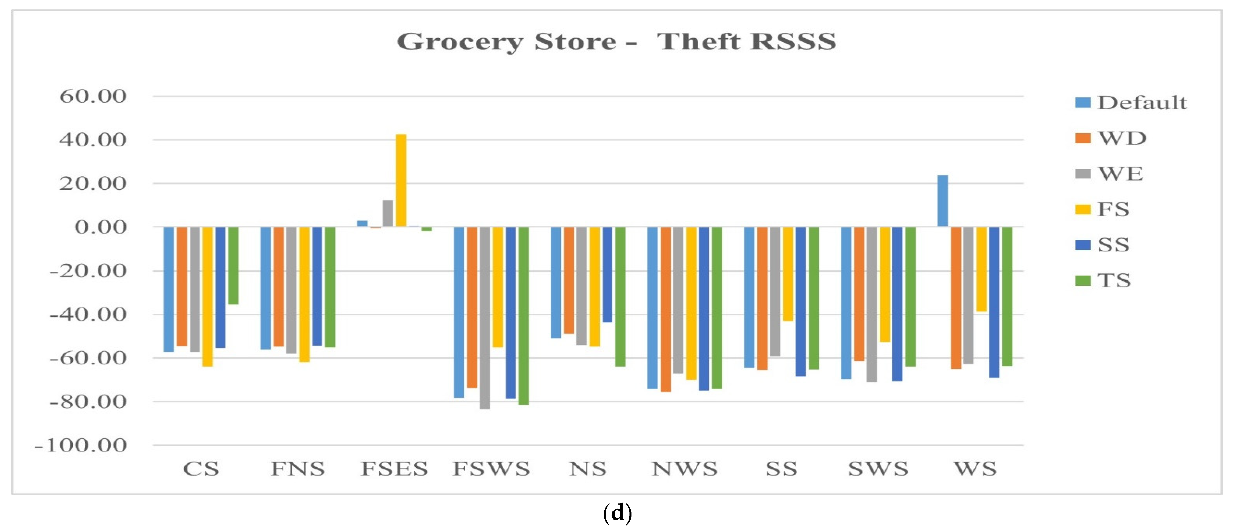
| Grocery Store | Center | −38.82 | −30.43 | −47.26 | −34.95 | −11.55 | −50.02 | −57.06 | −54.56 | −57.07 | −64.00 | −55.43 | −35.39 |
| Far North | −44.10 | −44.09 | −44.07 | −42.25 | −59.23 | −30.88 | −55.96 | −54.74 | −58.15 | −61.85 | −54.28 | −55.08 | |
| Far South East | 7.66 | 36.23 | −23.35 | −38.53 | −16.73 | 46.00 | 2.97 | −0.41 | 12.39 | 42.60 | 0.70 | −1.86 | |
| Far South West | −35.46 | −43.76 | 2.67 | 3.42 | −12.62 | −45.93 | −78.20 | −73.70 | −83.50 | −55.05 | −78.63 | −81.33 | |
| North | −35.67 | −36.30 | −42.33 | −13.95 | −78.56 | −67.46 | −50.99 | −48.93 | −53.94 | −54.75 | −43.71 | −63.92 | |
| North West | −47.19 | −44.30 | −52.40 | 0.00 | −53.02 | −45.29 | −74.30 | −75.51 | −66.95 | −69.98 | −74.77 | −74.21 | |
| South | −55.03 | −52.92 | −56.25 | −57.65 | −58.44 | −50.46 | −64.66 | −65.51 | −59.17 | −43.02 | −68.37 | −65.18 | |
| South West | −35.86 | −46.74 | −11.97 | −15.98 | −46.97 | −37.08 | −69.82 | −61.37 | −71.04 | −52.61 | −70.72 | −63.83 | |
| West | 129.55 | −33.88 | −50.45 | −20.03 | −47.05 | −42.43 | 23.75 | −64.93 | −62.82 | −38.87 | −69.00 | −63.67 | |
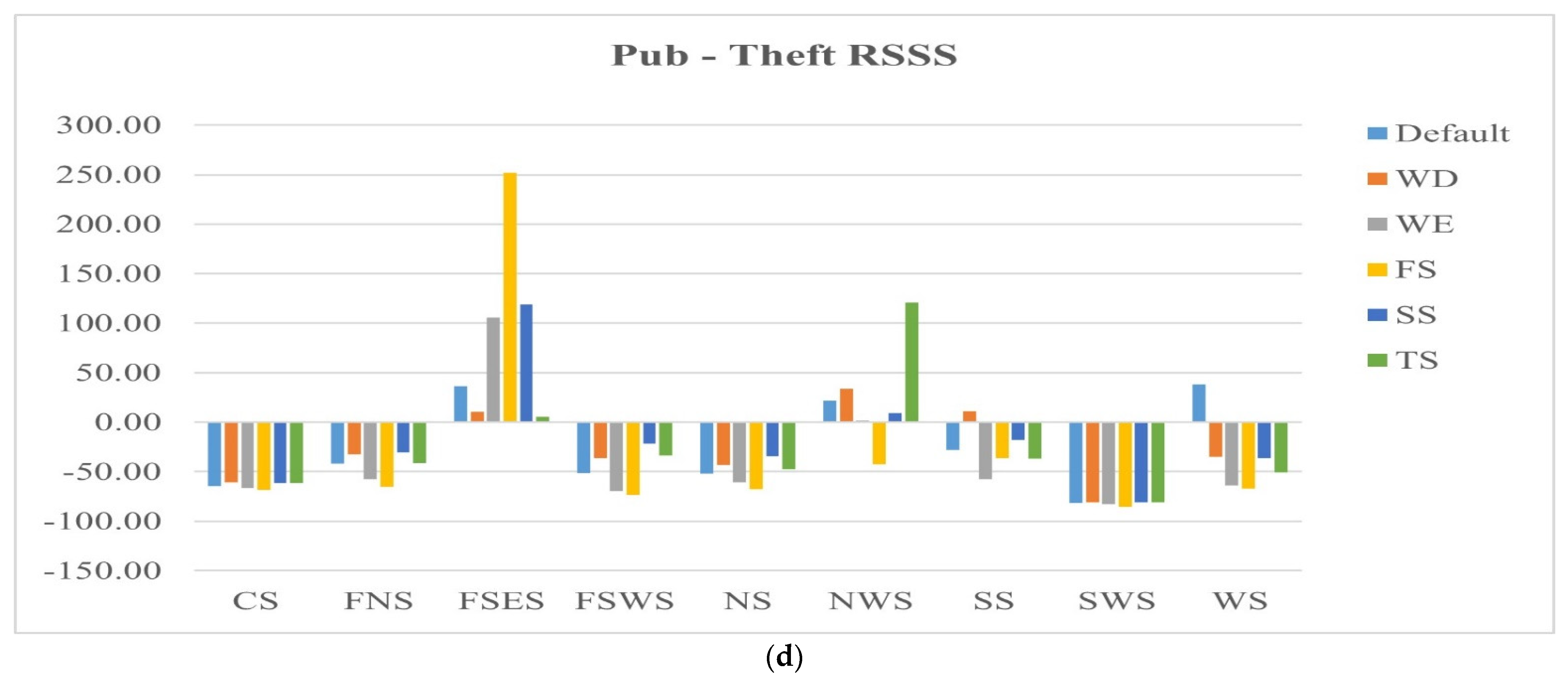
| Pub/Taverns | Center | −45.66 | −22.87 | −53.52 | −52.01 | −41.13 | −32.50 | −64.51 | −60.45 | −66.64 | −68.30 | −61.48 | −61.47 |
| Far North | −38.69 | −40.99 | −30.96 | −46.71 | −32.97 | −27.13 | −41.93 | −32.52 | −57.66 | −65.24 | −30.36 | −40.95 | |
| Far South East | 8.73 | 91.32 | −37.52 | −40.00 | 677.99 | −23.79 | 36.42 | 10.31 | 105.73 | 251.67 | 119.07 | 5.60 | |
| Far South West | −32.01 | 0.00 | −22.26 | −71.84 | 0.00 | 89.16 | −51.35 | −35.89 | −69.66 | −73.16 | −21.81 | −33.89 | |
| North | −36.62 | −9.79 | −57.76 | −50.49 | −54.80 | −16.92 | −51.75 | −43.14 | −60.49 | −67.54 | −34.46 | −47.46 | |
| North West | −65.86 | −71.38 | −56.39 | −71.88 | 43.83 | −73.14 | 21.96 | 34.09 | 1.73 | −42.16 | 8.97 | 120.68 | |
| South | 129.35 | 112.56 | 0.00 | 0.00 | 30.94 | 304.44 | −27.92 | 11.37 | −57.40 | −35.98 | −17.83 | −36.72 | |
| South West | −9.44 | −35.20 | 0.00 | 0.00 | −30.61 | 0.00 | −81.58 | −81.08 | −82.51 | −85.09 | −80.62 | −80.81 | |
| West | 188.85 | 0.00 | −57.35 | −18.97 | 0.00 | −38.86 | 38.08 | −35.20 | −63.97 | −66.79 | −35.91 | −50.76 | |
References
- Ratcliffe, J.H. The Spatial Extent of Criminogenic Places: A Changepoint Regression of Violence around Bars. Geogr. Anal. 2012, 44, 302–320. [Google Scholar] [CrossRef]
- Groff, E.R. Measuring a place’s exposure to facilities using geoprocessing models: An illustration using drinking places and crime. In Crime Modeling and Mapping Using Geospatial Technologies; Leitner, M., Ed.; Springer: Dordrecht, The Netherlands, 2013; pp. 269–295. [Google Scholar] [CrossRef]
- Groff, E.R.; Lockwood, B. Criminogenic Facilities and Crime across Street Segments in Philadelphia. J. Res. Crime Delinq. 2014, 51, 277–314. [Google Scholar] [CrossRef]
- Groff, E. Exploring ‘near’: Characterizing the spatial extent of drinking place influence on crime. Aust. N. Z. J. Criminol. 2011, 44, 156–179. [Google Scholar] [CrossRef]
- Wheeler, A.P. Quantifying the Local and Spatial Effects of Alcohol Outlets on Crime. Crime Delinquency 2019, 65, 845–871. [Google Scholar] [CrossRef]
- Cohen, L.E.; Felson, M. Social Change and Crime Rate Trends: A Routine Activity Approach. Am. Sociol. Rev. 1979, 44, 588. [Google Scholar] [CrossRef]
- Brantingham, P.J.; Brantingham, P.L. Environmental Criminology; Sage Publications: Beverly Hills, CA, USA, 1981. [Google Scholar]
- Brantingham, P.L.; Brantingham, P.J. Nodes, paths and edges: Considerations on the complexity of crime and the physical environment. J. Environ. Psychol. 1993, 13, 3–28. [Google Scholar] [CrossRef]
- Brantingham, P.; Brantingham, P. Criminality of place. Eur. J. Crim. Policy Res. 1995, 3, 5–26. [Google Scholar] [CrossRef]
- Eck, J.E.; Clarke, R.V.; Guerette, R.T. Risky facilities: Crime concentration in homogeneous sets of establishments and facilities. Crime Prevention Studies 2007, 21, 225–264. [Google Scholar]
- Timms, D. The Urban Mosaic: Towards a Theory of Residential Differentiation, 2nd ed.; CUP Archive: Cambridge, UK, 1975. [Google Scholar]
- Pred, A. Social Reproduction and the Time-Geography of Everyday Life. Geogr. Ann. Ser. B Hum. Geogr. 1981, 63, 5. [Google Scholar] [CrossRef]
- Hägerstraand, T. What about people in regional science? Pap. Reg. Sci. 1970, 24, 7–24. [Google Scholar] [CrossRef]
- Jacobs, J. The Death and Life of Great American Cities; Vintage: New York, NY, USA, 1961. [Google Scholar]
- Stucky, T.D.; Ottensmann, J.R. Land use and violent crime. Criminology 2009, 47, 1223–1264. [Google Scholar] [CrossRef] [Green Version]
- Browning, C.R.; Byron, R.A.; Calder, C.A.; Krivo, L.J.; Kwan, M.-P.; Lee, J.-Y.; Peterson, R.D. Commercial Density, Residential Concentration, and Crime: Land Use Patterns and Violence in Neighborhood Context. J. Res. Crime Delinq. 2010, 47, 329–357. [Google Scholar] [CrossRef]
- Clarke, R.V. Situational Crime Prevention. Crime Justice 1995, 19, 91–150. [Google Scholar] [CrossRef]
- Kinney, J.B.; Brantingham, P.L.; Wuschke, K.; Kirk, M.G.; Brantingham, P.J. Crime Attractors, Generators and Detractors: Land Use and Urban Crime Opportunities. Built Environ. 2008, 34, 62–74. [Google Scholar] [CrossRef]
- Loukaitou-Sideris, A. Hot Spots of Bus Stop Crime. J. Am. Plan. Assoc. 1999, 65, 395–411. [Google Scholar] [CrossRef]
- Roncek, D.W.; Pravatiner, M.A. Additional evidence that taverns enhance nearby crime. Sociol. Soc. Res. 1989, 73, 185–188. [Google Scholar]
- Roncek, D.W.; Maier, P.A. Bars, blocks, and crimes revisited: Linking the theory of routine activities to the empiricism of "hot spots". Criminology 1991, 29, 725–753. [Google Scholar] [CrossRef]
- Rengert, G.F.; Piquero, A.R.; Jones, P.R. DISTANCE DECAY REEXAMINED. Criminology 1999, 37, 427–446. [Google Scholar] [CrossRef]
- Rice, K.J.; Csmith, W.R. Socioecological Models of Automotive Theft: Integrating Routine Activity and Social Disorganization Approaches. J. Res. Crime Delinq. 2002, 39, 304–336. [Google Scholar] [CrossRef]
- Weisburd, D.; Groff, E.R.; Yang, S.M. The Criminology of Place: Street Segments and Our Understanding of the Crime Problem; Oxford University Press: Oxford, UK, 2012. [Google Scholar]
- Rengert, G.F.; Ratcliffe, J.; Chakravorty, S. Policing Illegal Drug Markets: Geographic Approaches to Crime Reduction; Criminal Justice Press: Monsey, NY, USA, 2005. [Google Scholar]
- Newton, A.; Hirschfield, A. Measuring violence in and around licensed premises: The need for a better evidence base. Crime Prev. Community Saf. 2009, 11, 171–188. [Google Scholar] [CrossRef] [Green Version]
- Mccord, E.S.; Ratcliffe, J.H. A Micro-Spatial Analysis of the Demographic and Criminogenic Environment of Drug Markets in Philadelphia. Aust. N. Z. J. Criminol. 2007, 40, 43–63. [Google Scholar] [CrossRef] [Green Version]
- Xu, J.; Griffiths, E. Shooting on the Street: Measuring the Spatial Influence of Physical Features on Gun Violence in a Bounded Street Network. J. Quant. Criminol. 2017, 33, 237–253. [Google Scholar] [CrossRef]
- Felson, M.; Boivin, R. Daily crime flows within a city. Crime Sci. 2015, 4, 31. [Google Scholar] [CrossRef] [Green Version]
- Bernasco, W.; Block, R. Robberies in Chicago: A Block-Level Analysis of the Influence of Crime Generators, Crime Attractors, and Offender Anchor Points. J. Res. Crime Delinq. 2010, 48, 33–57. [Google Scholar] [CrossRef]
- Yamada, I.; Thill, J.-C. Comparison of planar and network K-functions in traffic accident analysis. J. Transp. Geogr. 2004, 12, 149–158. [Google Scholar] [CrossRef]
- Lu, Y.; Chen, X. On the false alarm of planar K-function when analyzing urban crime distributed along streets. Soc. Sci. Res. 2007, 36, 611–632. [Google Scholar] [CrossRef]
- Tompson, L.; Partridge, H.; Shepherd, N. Hot routes: Developing a new technique for the spatial analysis of crime. Crime Mapp. J. Res. Pract. 2009, 1, 77–96. [Google Scholar]
- Maki, N.; Okabe, A. A Spatio-Temporal Analysis of Aged Members of a Fitness Club in a Suburb. Proc. Geogr. Inf. Syst. Assoc. 2005, 14, 29–34. [Google Scholar]
- Groff, E.R. Measuring the Influence of the Built Environment on Crime at Street Segments. Jerus. Rev. Leg. Stud. 2017, 15, 44–54. [Google Scholar] [CrossRef]
- Ratcliffe, J. A Temporal Constraint Theory to Explain Opportunity-Based Spatial Offending Patterns. J. Res. Crime Delinq. 2006, 43, 261–291. [Google Scholar] [CrossRef]
- Haberman, C.P.; Ratcliffe, J. Testing for temporally differentiated relationships among potentially criminogenic places and census block street robbery counts. Criminology 2015, 53, 457–483. [Google Scholar] [CrossRef]
- Bernasco, W.; Ruiter, S.; Block, R. Do Street Robbery Location Choices Vary Over Time of Day or Day of Week? A Test in Chicago. J. Res. Crime Delinq. 2017, 54, 244–275. [Google Scholar] [CrossRef] [PubMed]
- Corcoran, J.; Zahnow, R.; Kimpton, A.; Wickes, R.; Brunsdon, C. The temporality of place: Constructing a temporal typology of crime in commercial precincts. Environ. Plan. B Urban Anal. City Sci. 2021, 48, 9–24. [Google Scholar] [CrossRef]
- Irvin-Erickson, Y.; La Vigne, N. A Spatio-temporal Analysis of Crime at Washington, DC Metro Rail: Stations’ Crime-generating and Crime-attracting Characteristics as Transportation Nodes and Places. Crime Sci. 2015, 4, 14. [Google Scholar] [CrossRef]
- Hart, T.C.; Miethe, T.D. Configural Behavior Settings of Crime Event Locations. J. Res. Crime Delinq. 2015, 52, 373–402. [Google Scholar] [CrossRef]
- MacDonald, J.M.; Nicosia, N.; Ukert, B.D. Do Schools Cause Crime in Neighborhoods? Evidence from the Opening of Schools in Philadelphia. J. Quant. Criminol. 2018, 34, 717–740. [Google Scholar] [CrossRef]
- Barnum, J.D.; Caplan, J.M.; Kennedy, L.W.; Piza, E.L. The crime kaleidoscope: A cross-jurisdictional analysis of place features and crime in three urban environments. Appl. Geogr. 2017, 79, 203–211. [Google Scholar] [CrossRef] [Green Version]
- Hipp, J.R.; Kim, Y.-A. Explaining the temporal and spatial dimensions of robbery: Differences across measures of the physical and social environment. J. Crim. Justice 2019, 60, 1–12. [Google Scholar] [CrossRef]
- Breetzke, G.D.; Edelstein, I.S. Do crime generators exist in a developing context? An exploratory study in the township of Khayelitsha, South Africa. Secur. J. 2020, 1–18. [Google Scholar] [CrossRef]
- McCord, E.S.; Ratcliffe, J.H. Intensity value analysis and the criminogenic effects of land use features on local crime patterns. Crime Patterns Anal. 2009, 2, 17–30. [Google Scholar]
- About Chicago: Facts and Statistics. Available online: https://www.chicago.gov/city/en/about/facts.html (accessed on 12 May 2021).
- The “Sides” of Chicago. Chicago Studies. Available online: https://chicagostudies.uchicago.edu/sides (accessed on 12 May 2021).
- Keating, A.D. Chicago Neighborhoods and Suburbs: A Historical Guide; University of Chicago Press: Chicago, IL, USA, 2008. [Google Scholar]
- Sampson, R.J. Great American City: Chicago and the Enduring Neighborhood Effect; University of Chicago Press: Chicago, IL, USA, 2012. [Google Scholar]
- Block, R. Street Gang Crime in Chicago; National Institute of Justice: Washington, DC, USA, 1993.
- Schnell, C.; Braga, A.A.; Piza, E.L. The Influence of Community Areas, Neighborhood Clusters, and Street Segments on the Spatial Variability of Violent Crime in Chicago. J. Quant. Criminol. 2017, 33, 469–496. [Google Scholar] [CrossRef] [Green Version]
- Okabe, A.; Sugihara, K. Spatial Analysis Along Networks: Statistical and Computational Methods; John Wiley and Sons: Hoboken, NJ, USA, 2012. [Google Scholar]
- Payroll and Timekeeping—Attendance. Available online: http://directives.chicagopolice.org/directives/data/a7a57b36-12cf4df7-24112-cf4e-9398046d4f55fbaf.html (accessed on 3 July 2021).
- Bernasco, W.; Block, R. Where offenders choose to attack: A discrete choice model of robberies in chicago. Criminology 2009, 47, 93–130. [Google Scholar] [CrossRef]
- Kennedy, L.W.; Caplan, J.M.; Piza, E.L.; Buccine-Schraeder, H. Vulnerability and Exposure to Crime: Applying Risk Terrain Modeling to the Study of Assault in Chicago. Appl. Spat. Anal. Policy 2016, 9, 529–548. [Google Scholar] [CrossRef] [Green Version]
- Kim, Y.-A. Examining the Relationship Between the Structural Characteristics of Place and Crime by Imputing Census Block Data in Street Segments: Is the Pain Worth the Gain? J. Quant. Criminol. 2016, 34, 67–110. [Google Scholar] [CrossRef]
- Okabe, A.; Yamada, I. The K-Function Method on a Network and Its Computational Implementation. Geogr. Anal. 2010, 33, 271–290. [Google Scholar] [CrossRef]
- Ripley’s K Function. Wiley StatsRef: Statistics Reference. Available online: https://0-onlinelibrary-wiley-com.brum.beds.ac.uk/doi/abs/10.1002/9781118445112.stat07751 (accessed on 12 May 2021).
- Baddeley, A.; Diggle, P.J.; Hardegen, A.; Lawrence, T.; Milne, R.K.; Nair, G. On tests of spatial pattern based on simulation envelopes. Ecol. Monogr. 2014, 84, 477–489. [Google Scholar] [CrossRef] [Green Version]
- Baddeley, A.J.; Turner, R. Spatstat: An R package for analyzing spatial point pattens. J. Stat. Softw. 2005, 12, 1–42. [Google Scholar] [CrossRef] [Green Version]
- Kim, H.-J.; Fay, M.P.; Feuer, E.J.; Midthune, D.N. Permutation tests for joinpoint regression with applications to cancer rates. Stat. Med. 2000, 19, 335–351. [Google Scholar] [CrossRef]
- Nelessen, A.C. Visions for a New American Dream; Planners Press, American Planning Association: Chicago, IL, USA, 1994. [Google Scholar]
- Caplan, J.M. Mapping the spatial influence of crime correlates: A comparison of operationalization schemes and implications for crime analysis and criminal justice practice. Cityscape 2011, 13, 57–83. [Google Scholar]
- He, Z.; Deng, M.; Xie, Z.; Wu, L.; Chen, Z.; Pei, T. Discovering the joint influence of urban facilities on crime occurrence using spatial co-location pattern mining. Cities 2020, 99, 102612. [Google Scholar] [CrossRef]
- A Andresen, M.; Malleson, N. Intra-week spatial-temporal patterns of crime. Crime Sci. 2015, 4, 12. [Google Scholar] [CrossRef]
- Yue, H.; Zhu, X.; Ye, X.; Guo, W. The Local Colocation Patterns of Crime and Land-Use Features in Wuhan, China. ISPRS Int. J. Geo-Inform. 2017, 6, 307. [Google Scholar] [CrossRef] [Green Version]
- Feng, S.Q.; Piza, E.L.; Kennedy, L.W.; Caplan, J.M. Aggravating effects of alcohol outlet types on street robbery and aggravated assault in New York City. J. Crime Justice 2018, 42, 257–273. [Google Scholar] [CrossRef]
- Song, G.; Bernasco, W.; Liu, L.; Xiao, L.; Zhou, S.; Liao, W. Crime Feeds on Legal Activities: Daily Mobility Flows Help to Explain Thieves’ Target Location Choices. J. Quant. Criminol. 2019, 35, 831–854. [Google Scholar] [CrossRef] [Green Version]
- De Melo, S.N.; Pereira, D.V.S.; Andresen, M.A.; Matias, L. Spatial/Temporal Variations of Crime: A Routine Activity Theory Perspective. Int. J. Offender Ther. Comp. Criminol. 2018, 62, 1967–1991. [Google Scholar] [CrossRef] [PubMed]
- Jeffery, C.R. Crime Prevention through Environmental Design; Sage Publications: Beverly Hills, CA, USA, 1971. [Google Scholar]
- Xu, Y.; Fu, C.; Kennedy, E.; Jiang, S.; Owusu-Agyemang, S. The impact of street lights on spatial-temporal patterns of crime in Detroit, Michigan. Cities 2018, 79, 45–52. [Google Scholar] [CrossRef]
- Wong, D. The modifiable areal unit problem (MAUP). In SAGE Handbook of Spatial Analysis; Fotheringham, A., Rogerson, P.A., Eds.; Sage Publications: Thousand Oaks, CA, USA, 2009; pp. 105–123. [Google Scholar]
- Cheng, T.; Adepeju, M. Modifiable Temporal Unit Problem (MTUP) and Its Effect on Space-Time Cluster Detection. PLoS ONE 2014, 9, e100465. [Google Scholar] [CrossRef] [Green Version]
- Fox, B.; Trolard, A.; Simmons, M.; Meyers, J.E.; Vogel, M. Assessing the Differential Impact of Vacancy on Criminal Violence in the City of St. Louis, MO. Crim. Justice Rev. 2021, 46, 156–172. [Google Scholar] [CrossRef]


| Sides | #Nodes | #Edges | Bounding Box Coordinates | Bounding Radius (m) | Network K Distance Chunks (m) |
|---|---|---|---|---|---|
| C | 1680 | 2444 | (41.91, −87.60; 41.84, −87.65) | 9977.9 | 19.4 |
| FN | 5407 | 8151 | (42.02, −87.63; 41.93, −87.93) | 29,611.9 | 57.7 |
| FSE | 4873 | 7227 | (41.75, −87.52; 41.64, −87.66) | 20,438.6 | 39.8 |
| FSW | 3509 | 5308 | (41.75, −87.63; 41.66, −87.74) | 15,932.5 | 31.0 |
| N | 2691 | 4145 | (41.96, −87.62; 41.91, −87.73) | 14,001.2 | 27.2 |
| NW | 2693 | 4423 | (41.96, −87.69; 41.91, −87.83) | 16,737.1 | 32.6 |
| S | 4040 | 6023 | (41.85, −87.54; 41.74, −87.66) | 15,770 | 30.7 |
| SW | 5032 | 7976 | (41.78, −87.62; 41.75, −87.80) | 17,380.9 | 33.8 |
| W | 6762 | 10,395 | (41.92, −87.63; 41.81, −87.80) | 20,760.5 | 40.4 |
| Mean | SD | Eigen Value | Factor Loadings | Cronbach’s Alpha | |
|---|---|---|---|---|---|
| Concentrated Disadvantage (CD) | 0.000 | 1 | 3.105 | 0.901 | |
| % under 15 above 64 years | 38.074 | 6.545 | 0.753 | ||
| % unemployed | 5.973 | 3.075 | 0.907 | ||
| % less than poverty | 29.936 | 13.964 | 0.925 | ||
| Inverted median income | 51,038.798 | 23,754.78 | 0.926 |
Publisher’s Note: MDPI stays neutral with regard to jurisdictional claims in published maps and institutional affiliations. |
© 2021 by the authors. Licensee MDPI, Basel, Switzerland. This article is an open access article distributed under the terms and conditions of the Creative Commons Attribution (CC BY) license (https://creativecommons.org/licenses/by/4.0/).
Share and Cite
Hakyemez, T.C.; Badur, B. Crime Risk Stations: Examining Spatiotemporal Influence of Urban Features through Distance-Aware Risk Signal Functions. ISPRS Int. J. Geo-Inf. 2021, 10, 472. https://0-doi-org.brum.beds.ac.uk/10.3390/ijgi10070472
Hakyemez TC, Badur B. Crime Risk Stations: Examining Spatiotemporal Influence of Urban Features through Distance-Aware Risk Signal Functions. ISPRS International Journal of Geo-Information. 2021; 10(7):472. https://0-doi-org.brum.beds.ac.uk/10.3390/ijgi10070472
Chicago/Turabian StyleHakyemez, Tugrul Cabir, and Bertan Badur. 2021. "Crime Risk Stations: Examining Spatiotemporal Influence of Urban Features through Distance-Aware Risk Signal Functions" ISPRS International Journal of Geo-Information 10, no. 7: 472. https://0-doi-org.brum.beds.ac.uk/10.3390/ijgi10070472