A3T-GCN: Attention Temporal Graph Convolutional Network for Traffic Forecasting

Abstract

Accurate real-time traffic forecasting is a core technological problem against the implementation of the intelligent transportation system. However, it remains challenging considering the complex spatial and temporal dependencies among traffic flows. In the spatial dimension, due to the connectivity of the road network, the traffic flows between linked roads are closely related. In the temporal dimension, although there exists a tendency among adjacent time points, the importance of distant time points is not necessarily less than that of recent ones, since traffic flows are also affected by external factors. In this study, an attention temporal graph convolutional network (A3T-GCN) was proposed to simultaneously capture global temporal dynamics and spatial correlations in traffic flows. The A3T-GCN model learns the short-term trend by using the gated recurrent units and learns the spatial dependence based on the topology of the road network through the graph convolutional network. Moreover, the attention mechanism was introduced to adjust the importance of different time points and assemble global temporal information to improve prediction accuracy. Experimental results in real-world datasets demonstrate the effectiveness and robustness of the proposed A3T-GCN. We observe the improvements in RMSE of 2.51–46.15% and 2.45–49.32% over baselines for the SZ-taxi and Los-loop, respectively. Meanwhile, the Accuracies are 0.95–89.91% and 0.26–10.37% higher than the baselines for the SZ-taxi and Los-loop, respectively.

1. Introduction

Traffic forecasting is an important component of intelligent transportation systems and a vital part of transportation planning and management, and traffic control [1,2,3,4]. Accurate real-time traffic forecasting has been a great challenge because of complex spatiotemporal dependencies. Temporal dependence means that the traffic state changes with time, which is manifested by periodicity and tendency. Spatial dependence means that changes in traffic state are subject to the structural topology of road networks, which is manifested by the transmission of the upstream traffic state to downstream sections and the retrospective effects of the downstream traffic state on the upstream section [5]. Hence, considering the complex temporal features and the topological characteristics of the road network is essential for realizing the traffic forecasting task.

Existing traffic forecasting models can be divided into parametric models and non-parametric models. Common parametric models include historical average, time series [6,7], linear regression [8], and Kalman filtering models [9]. Although traditional parametric models use simple algorithms, they depend on stationary hypotheses. These models can neither reflect non-linearity and the uncertainty of traffic states nor overcome the interference of random events, such as traffic accidents. Non-parametric models can solve these problems well because they can learn the statistical laws of data automatically with adequate historical data. Common non-parametric models include k-nearest [10], support vector regression (SVR) [11,12], fuzzy logic [13], Bayesian network [14], and neural network models [15].

Recently, deep neural network models have attracted widespread attention from scholars because of the rapid development of deep learning [16,17,18]. Recurrent neural networks (RNNs), long short-term memory (LSTM) [19], and gated recurrent units (GRUs) [20] have been successfully utilized in traffic forecasting because they can use self-circulation mechanisms and model temporal dependence [21,22,23]. However, these models only consider the temporal variation of the traffic state and neglect spatial dependence. Many scholars have introduced convolutional neural networks (CNNs) in their models to characterize spatial dependence. Wu et al. [24] designed a feature fusion framework for short-term traffic flow forecasting by combining a CNN with LSTM. The framework captured the spatial characteristics of traffic flow through a one-dimensional CNN and explored short-term variations and the periodicity of traffic flow with two LSTMs. Cao et al. [25] proposed an end-to-end model called Interactive Temporal Recurrent Convolution Network (ITRCN), which transformed the interactive network flow to images and captured network flows using a CNN. ITRCN also extracted temporal features by using GRU. An experiment proved that the forecasting error of this method was 14.3% and 13.0% higher than those of GRU and CNN, respectively. Yu et al. [26] captured spatial correlation and temporal dynamics by the spatiotemporal recurrent convolutional networks (SRCN) based on deep convolutional neural network (DCNN) and LSTM. They also proved the superiority of SRCN based on the investigation of the traffic network data in Beijing. Sun et al. [27] proposed a deep-learning-based multi-branch model called Traffic Flow Forecasting Network (TFFNet) to forecast the short-term traffic flow. The TFFNet employed a multilayer fully convolutional framework to extract the hierarchical spatial dependencies from local to global scales.

Although CNN is applicable to Euclidean data [28], such as image and grids, it still has limitations in traffic networks, which possess non-Euclidean structures. In recent years, graph convolutional network (GCN) [29], which can overcome the abovementioned limitations and capture the structural characteristics of networks, has rapidly developed [30,31,32]. In addition, RNNs and their variants use sequential processing over time and are more apt to remember the latest information, thus are suitable for capturing evolving short-term tendencies. However, one problem with these models is that their performance will decrease as the prediction horizon increases. Moreover, the importance of different time points cannot be distinguished only by the proximity of time. As Pavlyuk suggested in [33], the definition of the spatiotemporal structure of traffic flow should also include relationships that are distant in time. Long-term dependencies (e.g., periodical dependencies) hidden in large time spans should be considered. Therefore, mechanisms that are capable of learning global correlations in long input time sequences are needed.

For this reason, an attention temporal GCN (A3T-GCN) was proposed for the traffic forecasting task. The A3T-GCN combines GCNs and GRUs and introduces an attention mechanism [34,35]. It can not only capture spatiotemporal dependencies but also adjust and assemble global variation information. The A3T-GCN is used for traffic forecasting on the basis of urban road networks.

The rest of the paper is organized as follows. Section 2 introduces the proposed model. In Section 3, we evaluate the performance of the A3T-GCN with real-world traffic datasets, including prediction results analysis, perturbation analysis, and visualization interpretation. We conclude the paper in Section 4.

2. Methods

2.1. Definition of Problems

In this study, traffic forecasting is performed to predict future traffic states according to historical traffic states on urban roads. Generally, traffic state can refer to traffic flow, speed, and density. In this study, traffic state only refers to traffic speed.

Definition 1.

Road network G: The topological structure of the urban road network is described as $G=(V,E)$, where $V=\{v_1,v_2,\cdots ,v_N\}$ is the set of the road sections and N is the number of road sections. E is the set of edges, which reflects the connections between road sections. All of the connectivity information is stored in the adjacent matrix $A\in R^{N\times N}$, where rows and columns are indexed by road sections, and the value of each entry indicates the connectivity between corresponding road sections. The entry value is zero if there is no link between roads and one (unweighted graph) or non-negative (weighted graph) if otherwise.

Definition 2.

Feature matrix $X^{N\times P}$: Traffic speed on a road section is viewed as the attribute of network nodes and it is expressed by the feature matrix $X\in R^{N\times P}$, where P is the number of node attribute features, that is, the length of the historical time series. $X_i$ denotes the traffic speed in all sections at time i.

Therefore, the traffic forecasting, modelling temporal and spatial dependencies, can be viewed as learning a mapping function f on the basis of the road network G and feature matrix X of the road network. Traffic speeds of future T moments are calculated as follows:

$$\left[X_{t+1},\cdots ,X_{t+T}\right]=f\left(G;\left(X_{t-n},\cdots ,X_{t-1},X_t\right)\right),$$

(1)

where n is the length of a given historical time series and T is the length of time series that needs to be forecasted.

2.2. GCN Model

GCNs are semi-supervised models that can process graph structures. They are an advancement of CNNs in graph fields. GCNs have achieved much progress in many applications, such as image classification [36], document classification [28], and unsupervised learning [29]. Convolutional mode in GCNs includes spectrum and spatial domain convolutions [36]. The former was applied in this study. Spectrum convolution can be defined as the product of signal x on the graph and figure filter $g_{\theta }\left(L\right)$, which is constructed in the Fourier domain: $g_{\theta }\left(L\right)\ast x=U{g}_{\theta }\left(U^{T}x\right)$, where $\theta$ is a model parameter, L is the graph Laplacian matrix, U is the eigenvector of normalized Laplacian matrix $L=I_N-D^{-\frac{1}{2}}A{D}^{-\frac{1}{2}}=U\lambda U^T$, and $U^{T}x$ is the graph Fourier transformation of x. x can also be promoted to $X\in R^{N\times C}$, where C refers to the number of features.

Given the characteristic matrix X and adjacent matrix A, GCNs can replace the convolutional operation in anterior CNNs by performing the spectrum convolutional operation with consideration of the graph node and the first-order adjacent domains of nodes to capture the spatial characteristics of the graph. Moreover, a hierarchical propagation rule is applied to superpose multiple networks. A multilayer GCN model in [29] is expressed as:

$$H^{\left(l+1\right)}=\sigma \left({\tilde{D}}^{-\frac{1}{2}} \widehat{A} {\tilde{D}}^{-\frac{1}{2}} H^{\left(l\right)} {\theta }^{\left(l\right)}\right),$$

(2)

where $\tilde{A}=A+I_N$ is an adjacent matrix with self-connection structures, $I_N$ is an identity matrix, $\tilde{D}$ is a degree matrix, ${\tilde{D}}_{ii}={\sum }_j{\tilde{A}}_{ij}$, $H^{\left(l\right)}\in R^{N\times l}$ is the output of layer l, ${\theta }^{\left(l\right)}$ is the parameter of layer l, and $\sigma \left(·\right)$ is an activation function used for nonlinear modeling.

Generally, a two-layer GCN model [29] can be expressed as:

$$f\left(X,A\right)=\sigma \left(\widehat{A} ReLU\left(\widehat{A} X W_0\right)W_1\right),$$

(3)

where X is a feature matrix; A is the adjacent matrix; and $\widehat{A}={\tilde{D}}^{-\frac{1}{2}} \tilde{A} {\tilde{D}}^{-\frac{1}{2}}$ is a preprocessing step, where $\tilde{A}=A+I_N$ is the adjacent matrix of graph G with a self-connection structure. $W_0\in R^{P\times H}$ is the weight matrix from the input layer to the hidden unit layer, where P is the length of time and H is the number of hidden units. $W_1\in R^{H\times T}$ is the weight matrix from the hidden layer to the output layer. $f\left(X,A\right)\in R^{N\times T}$ denotes the output with a forecasting length of T, and $ReLU\left(\right)$ is a common nonlinear activation function.

GCNs can encode the topological structures of road networks and the attributes of road sections simultaneously by determining the topological relationship between the central road section and the surrounding road sections. Spatial dependence can be captured on this basis. In a word, this study learned spatial dependence through the GCN model [29].

2.3. GRU Model

Temporal dependence of traffic state is another key problem that hinders traffic forecasting. RNNs are neural network models that process sequential data. However, limitations in long-term forecasting are observed in traditional RNNs because of disadvantages in terms of gradient disappearance and explosion [37]. LSTM [19] and GRUs [20] are variants of RNNs that mediate the problems effectively. LSTM and GRUs have basically the same fundamental principles. Both models use gated mechanisms to maintain long-term information and perform similarly on various tasks [38]. Compared with GRUs, LSTM has an additional memory cell and adapts more gating units to control the information flow. Thus, GRU has a relatively simpler structure, fewer parameters, and is easier to compute and implement [39].

In the present model, temporal dependence was captured by a GRU model. The calculation process is introduced as follows, where $h_{t-1}$ is the hidden state at t − 1, $X_t$ is the traffic speed at the current moment, and $r_t$ is the reset gate to control the degree of neglecting the state information at the previous moment. Information irrelevant to forecasting can be abandoned. If the reset gate outputs 0, then the traffic information at the previous moment is neglected. If the reset gate outputs 1, then the traffic information at the previous moment is brought into the next moment completely. $u_t$ is the update gate and is used to control the state information quantity at the previous moment that is brought into the current state. Meanwhile, $c_t$ is the memory content stored at the current moment, and $h_t$ is the output state at the current moment.

$$u_t=\sigma (W_u\ast \left[X_t,h_{t-1}\right]+b_u)$$

(4)

$$r_t=\sigma (W_r\ast \left[X_t,h_{t-1}\right]+b_r)$$

(5)

$$c_t=tanh(W_c\left[X_t,(r_t\ast h_{t-1})\right]+b_c)$$

(6)

$$h_t=u_t\ast h_{t-1}+(1-u_t)\ast c_t.$$

(7)

GRUs determine the traffic state at the current moment by using the hidden state at the previous moment and traffic information at the current moment as input. GRUs retain the variation trends of historical traffic information when capturing traffic information at the current moment because of the gated mechanism. Hence, this model can capture dynamic temporal variation features from the traffic data, that is, this study has applied a GRU model to learn the temporal variation trends of the traffic state.

2.4. Attention Model

The attention model is realized on the basis of the encoder–decoder model. This model was initially used in neural machine translation tasks [40]. Nowadays, attention models are widely applied to image caption generation [34], recommendation systems [41] and document classification [42]. With the rapid development of such models, existing attention models can be divided into multiple types, such as soft and hard attention [40], global and local attention [43], and self-attention [35]. In the current study, a soft attention model was used to learn the importance of traffic information at every moment, and then a context vector that could express the global variation trends of the traffic state was calculated for future traffic forecasting tasks.

Suppose that a time series $X_i(i=1,2,\cdots ,n)$, where n is the time series length, is introduced. The design process of soft attention models is introduced as follows. First, the hidden states $h_i(i=1,2,\cdots ,n)$ at different moments are calculated using CNNs (and their variants) or RNNs (and their variant), and they are expressed as $H=\{h_1,h_2,\cdots ,h_n\}$. Second, a scoring function is designed to calculate the score/weight of each hidden state. Third, an attention function is designed to calculate the context vector $C_t$ that can describe global traffic variation information. Finally, the final output results are obtained using the context vector. In the present study, these steps were followed in the design process, but a multilayer perception was applied as the scoring function instead.

Particularly, the characteristics $h_i$ at each moment were used as input when calculating the weight of each hidden state based on the attention mechanism. The corresponding outputs could be gained through two hidden layers. The weights of each characteristic ${\alpha }_i$ were calculated by a Softmax normalized index function (Equation (8)), where $w_{\left(1\right)}$ and $b_{\left(1\right)}$ are the weight and deviation of the first layer and $w_{\left(2\right)}$ and $b_{\left(2\right)}$ are the weight and deviation of the second layer, respectively.

$$e_i=w_{\left(2\right)}(w_{\left(1\right)}H+b_{\left(1\right)})+b_{\left(2\right)}$$

(8)

$${\alpha }_i=\frac{exp\left(e_i\right)}{{\sum }_{k=1}^{n}exp\left(e_k\right)}.$$

(9)

Finally, the attention function was designed. The calculation process of the context vector $C_t$ that covers global traffic variation information is shown in Equation (10).

$$C_t={\displaystyle \sum _{i=1}^n}{\alpha }_i\ast h_i.$$

(10)

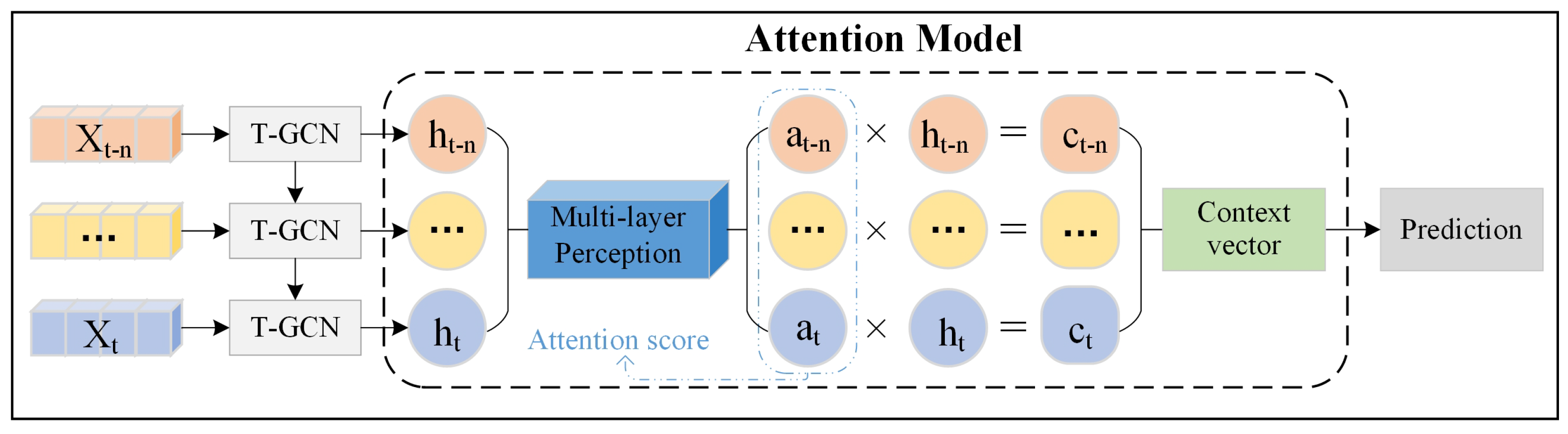
2.5. A3T-GCN Model

The A3t-GCN is an improvement of our previous work named the Temporal Graph Convolutional Network (T-GCN) [31]. The attention mechanism was introduced to re-weight the influence of historical traffic states and thus to capture the global variation trends of the traffic state. The model structure is shown in Figure 1.

The T-GCN model was constructed by combining GCN and GRU. First, n time steps of the historical traffic data were input into the T-GCN model to obtain n hidden states (h) that covered spatiotemporal characteristics: $\{h_{t-n},\cdots ,h_{t-1},h_t\}$. The calculation of the T-GCN is shown in Equations (11)–(14) [31], where $h_{t-1}$ is the output at t − 1. GC is the graph convolutional process. $u_t$ and $r_t$ are the update and reset gates at t, respectively. $c_t$ is the stored content at the current moment. $h_t$ is the output state at moment t, and W and b are the weight and the deviation in the training process, respectively.

$$u_t=\sigma (W_u\ast [GC(A,X_t),h_{t-1}]+b_u)$$

(11)

$$r_t=\sigma (W_r\ast [GC(A,X_t),h_{t-1}]+b_r)$$

(12)

$$c_t=tanh(W_c\ast [GC(A,X_t),(r_t\ast h_{t-1})]+b_c)$$

(13)

$$h_t=u_t\ast h_{t-1}+(1-u_t)\ast c_t).$$

(14)

Then, the hidden states were fed into the attention model to determine the context vector that covers the global traffic variation information. Particularly, the weight of each h was calculated by Softmax using a multilayer perception: $\{a_{t-n},\cdots ,a_{t-1},a_t\}$. The context vector that covers global traffic variation information was calculated by the weighted sum. Finally, forecasting results were outputted using the fully connected layer.

In sum, we proposed the A3T-GCN to realize traffic forecasting. The urban road network was constructed into a graph network and the traffic state on different sections was described as node attributes. The topological characteristics of the road network were captured by a GCN to obtain spatial dependence. The dynamic variation of node attributes was captured by a GRU to obtain the local temporal tendency of the traffic state. The global variation trend of the traffic state was then captured by the attention model, which was conducive to realizing accurate traffic forecasting.

2.6. Loss Function

Training aims to minimize errors between real and predicted speed in the road network. The real and predicted speeds on different sections at t are expressed by Y and $\widehat{Y}$, respectively. Therefore, the objective function of A3T-GCN is shown as follows. The first term aims to minimize the error between real and predicted speed. The second term $L_{reg}$ is a normalization term, which is conducive to avoid overfitting. $\lambda$ is a hyper-parameter.

$$loss=\Vert Y_t-\widehat{Y_t}\Vert +\lambda L_{reg}.$$

(15)

3. Experiments

3.1. Data Description

Two real-world traffic datasets, namely, the taxi trajectory dataset (SZ-taxi) in Shenzhen City and the loop detector dataset (Los-loop) in Los Angeles, were used. Both datasets are related to the traffic speed. Hence, traffic speed is viewed as the traffic information in the experiments. The SZ-taxi dataset is the taxi trajectory of Shenzhen from 1 January to 31 January 2015. In the present study, 156 major roads of Luohu District were selected as the study area, so the size of the SZ-taxi adjacency matrix is $156\times 156$. The Los-loop dataset was collected on the highway of Los Angeles County in real-time by loop detectors. A total of 207 sensors, along with their traffic speeds from 1 March to 7 March 2012, were selected. The size of the Los-loop adjacency matrix is thus $207\times 207$.

3.2. Evaluation Metrics

To evaluate the prediction performance of the model, the error between real traffic speed and predicted results is evaluated based on the metrics following [31]:

(1) Root Mean Squared Error (RMSE):

$$RMSE=\sqrt{\frac{1}{MN}{\displaystyle \sum _{j=1}^M\sum _{i=1}^N}{(y_i^j-\widehat{y_i^j})}^2}.$$

(16)

(2) Mean Absolute Error (MAE):

$$MAE=\frac{1}{MN}{\displaystyle \sum _{j=1}^M\sum _{i=1}^N}\left|y_i^j-\widehat{y_i^j}\right|.$$

(17)

(3) Accuracy:

$$Accuracy=1-\frac{\Vert Y-\widehat{Y}{\Vert }_F}{{\Vert Y\Vert }_F},$$

(18)

where F is the Frobenius norm, which calculates the square root of the sum of the absolute squares of elements in the matrix.

(4) Coefficient of Determination ($R^2$):

$$R^2=1-\frac{{\sum }_{j=1}^M{\sum }_{i=1}^N{(y_i^j-\widehat{y_i^j})}^2}{{\sum }_{j=1}^M{\sum }_{i=1}^N{(y_i^j-\overline{Y})}^2}.$$

(19)

(5) Explained Variance Score ($var$):

$$var=1-\frac{Var\left\{Y-\widehat{Y}\right\}}{Var\left\{Y\right\}},$$

(20)

where $y_i^j$ and $\widehat{y_i^j}$ are the real and predicted traffic information of temporal sample j on road i, respectively. N is the number of nodes on the road. M is the number of temporal samples. Y and $\widehat{Y}$ are the set of $y_i^j$ and $\widehat{y_i^j}$ respectively, and $\overline{Y}$ is the mean of Y.

Particularly, RMSE and MAE were used to measure prediction error. Small RMSE and MASE values reflect high prediction precision. Accuracy is used to measure forecasting precision, and a high accuracy value is preferred. $R^2$ and $var$ calculate the correlation coefficient, which measures the ability of the prediction result to represent the actual data: the larger the value is, the better the prediction effect is.

3.3. Experimental Result Analysis

The hyper-parameters of A3T-GCN include learning rate, epoch and the number of hidden units. In the experiment, learning rate and epoch were manually set, on the basis of experiences, as 0.001 and 5000 for both datasets, and parameters were randomly initialized from a normal distribution. We tested the model on different numbers of hidden units (8, 16, 32, 64, 100, 128) and chose the numbers that reported the best performance, that is, 64 for the SZ-taxi dataset and 100 for the Los-loop dataset.

In the present study, 80% of the traffic data were used as the training set, and the remaining 20% of the data were used as the test set. The traffic information in the next 15, 30, 45, and 60 min was predicted. The predicted results were compared with results from the historical average model (HA), the auto-regressive integrated moving average model (ARIMA), SVR, the GCN model, and the GRU model. The A3T-GCN was analyzed from the perspectives of precision, spatiotemporal prediction capabilities, long-term prediction capability and global feature capturing capability.

3.3.1. High Prediction Precision

Table 1. The prediction results of the A3T-GCN model and other baseline methods on the SZ-taxi dataset.

T	Metric	HA	ARIMA	SVR	GCN	GRU	A3T-GCN
	RMSE	4.2951	7.2406	4.1455	5.6596	3.9994	3.8989
	MAE	2.7815	4.9824	2.6233	4.2367	2.5955	2.6840
15 min	Accuracy	0.7008	0.4463	0.7112	0.6107	0.7249	0.7318
	$R^2$	0.8307	*	0.8423	0.6654	0.8329	0.8512
	var	0.8307	0.0035	0.8424	0.6655	0.8329	0.8512
	RMSE	4.2951	6.7899	4.1628	5.6918	4.0942	3.9228
	MAE	2.7815	4.6765	2.6875	4.2647	2.6906	2.7038
30 min	Accuracy	0.7008	0.3845	0.7100	0.6085	0.7184	0.7302
	$R^2$	0.8307	*	0.8410	0.6616	0.8249	0.8493
	var	0.8307	0.0081	0.8413	0.6617	0.8250	0.8493
	RMSE	4.2951	6.7852	4.1885	5.7142	4.1534	3.9461
	MAE	2.7815	4.6734	2.7359	4.2844	2.7743	2.7261
45 min	Accuracy	0.7008	0.3847	0.7082	0.6069	0.7143	0.7286
	$R^2$	0.8307	*	0.8391	0.6589	0.8198	0.8474
	var	0.8307	0.0087	0.8397	0.6590	0.8199	0.8474
	RMSE	4.2951	6.7708	4.2156	5.7361	4.0747	3.9707
	MAE	2.7815	4.6655	2.7751	4.3034	2.7712	2.7391
60 min	Accuracy	0.7008	0.3851	0.7063	0.6054	0.7197	0.7269
	$R^2$	0.8307	*	0.8370	0.6564	0.8266	0.8454
	var	0.8307	0.0111	0.8379	0.6564	0.8267	0.8454

* Means that the values are small enough to be negligible, indicating that the model’s prediction effect is poor.

and

Table 2. The prediction results of the A3T-GCN model and other baseline methods on the Los-loop dataset.

T	Metric	HA	ARIMA	SVR	GCN	GRU	A3T-GCN
	RMSE	7.4427	10.0439	6.0084	7.7922	5.2182	5.0904
	MAE	4.0145	7.6832	3.7285	5.3525	3.0602	3.1365
15 min	Accuracy	0.8733	0.8275	0.8977	0.8673	0.9109	0.9133
	$R^2$	0.7121	0.0025	0.8123	0.6843	0.8576	0.8653
	var	0.7121	*	0.8146	0.6844	0.8577	0.8653
	RMSE	7.4427	9.3450	6.9588	8.3353	6.2802	5.9974
	MAE	4.0145	7.6891	3.7248	5.6118	3.6505	3.6610
30 min	Accuracy	0.8733	0.8275	0.8815	0.8581	0.8931	0.8979
	$R^2$	0.7121	0.0031	0.7492	0.6402	0.7957	0.8137
	var	0.7121	*	0.7523	0.6404	0.7958	0.8137
	RMSE	7.4427	10.0508	7.7504	8.8036	7.0343	6.6840
	MAE	4.0145	7.6924	4.1288	5.9534	4.0915	4.1712
45 min	Accuracy	0.8733	0.8273	0.8680	0.8500	0.8801	0.8861
	$R^2$	0.7121	*	0.6899	0.5999	0.7446	0.7694
	var	0.7121	0.0035	0.6947	0.6001	0.7451	0.7705
	RMSE	7.4427	10.0538	8.4388	9.2657	7.6621	7.0990
	MAE	4.0145	7.6952	4.5036	6.2892	4.5186	4.2343
60 min	Accuracy	0.8733	0.8273	0.8562	0.8421	0.8694	0.8790
	$R^2$	0.7121	*	0.6336	0.5583	0.6980	0.7407
	var	0.7121	0.0036	0.5593	0.5593	0.6984	0.7415

* Means that the values are small enough to be negligible, indicating that the model’s prediction effect is poor.

show the comparisons of different models and two real datasets in terms of the prediction precision of various traffic speed lengths. We bold the optimal results in tables, and * means that the values are small enough to be negligible, indicating that the model’s prediction effect is poor. The prediction precision of neural network models (e.g., A3T-GCN and GRU) is higher than that of other models (e.g., HA, ARIMA, and SVR). With respect to the 15-min time series, the RMSE and accuracy of HA are approximately 9.22% higher and 4.24% lower than those of A3T-GCN, respectively. The RMSE and accuracy of ARIMA are approximately 46.15% higher and 39.01% lower than those of A3T-GCN, respectively. The RMSE and accuracy of SVR are approximately 5.95% higher and 2.81% lower than those of A3T-GCN, respectively. Compared with GRU, the RMSE and accuracy of HA are approximately 6.88% higher and 3.32% lower, respectively. The RMSE and accuracy of ARIMA are approximately 44.76% and 38.07%, respectively. The RMSE and accuracy of SVAR are approximately 3.52% and 1.87%, respectively. These results are mainly caused by the poor nonlinear fitting abilities of HA, ARIMA, and SVAR with regard to complicated, changing traffic data. Processing long-term non-stationary data is difficult when ARIMA is used. Moreover, ARIMA gains by averaging the errors of different sections. The data of some sections might greatly fluctuate to increase the final error. Hence, ARIMA shows the lowest forecasting accuracy.

Similar conclusions could be drawn for Los-loop. The A3T-GCN model can obtain the optimal prediction performance of all metrics in two real datasets, thus proving the validity and superiority of the A3T-GCN model in spatiotemporal traffic forecasting tasks.

3.3.2. Effectiveness of Modeling Both Spatial and Temporal Dependencies

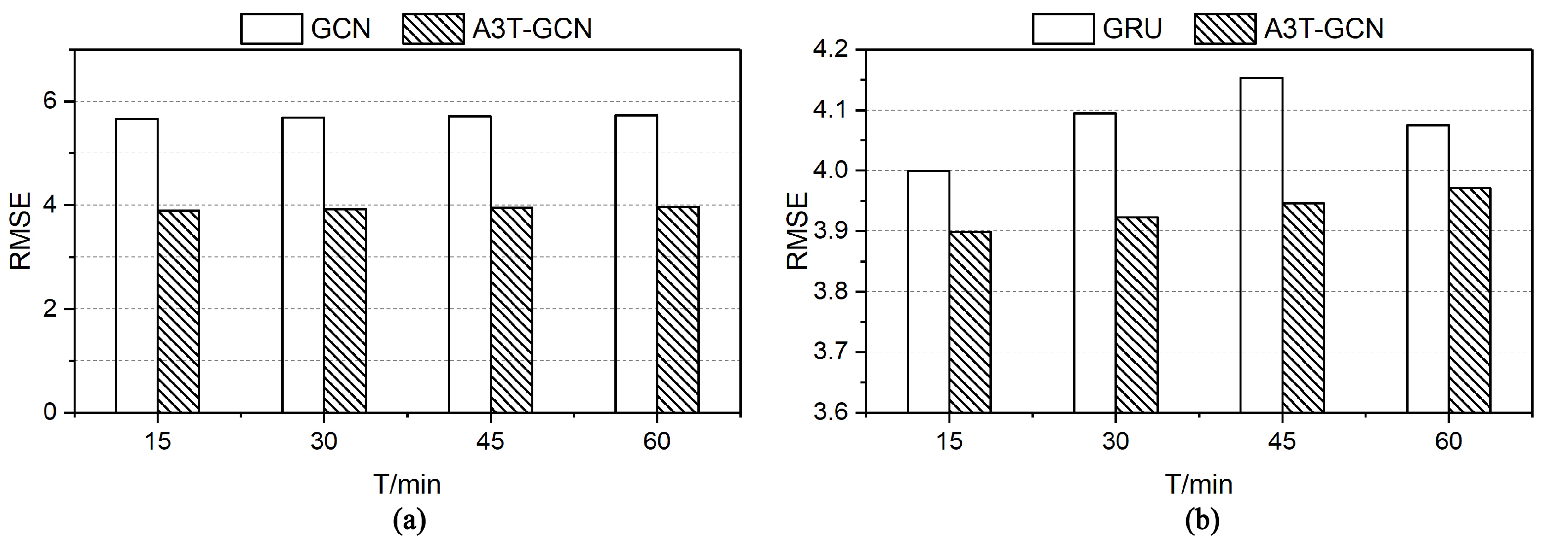
To test the benefits of depicting the spatiotemporal characteristics of traffic data simultaneously in A3T-GCN, the A3T-GCN model is compared with GCN and GRU.

Figure 2 shows the results based on SZ-taxi. The prediction error of A3T-GCN is kept lower than that of GCN (considering spatial characteristics only) in 15, 30, 45, and 60 min of traffic forecasting, as shown in Figure 2a. Compared with GCN, A3T-GCN achieves approximately 31.11%, 31.08%, 30.94%, and 30.78% lower RMSEs in 15, 30, 45, and 60 min of the traffic forecasting time series, respectively. Compared with GRU (considering temporal characteristics only), A3T-GCN achieves approximately 2.51% lower RMSE in 15 min traffic forecasting, approximately 4.19% lower RMSE in 30 min traffic forecasting, approximately 4.99% lower RMSE in the 45 min time series, and approximately 2.55% lower RMSE in the 60 min time series. In sum, the prediction error of A3T-GCN is kept lower than that of GRU in 15, 30, 45, and 60 min traffic forecasting, as shown in Figure 2b.

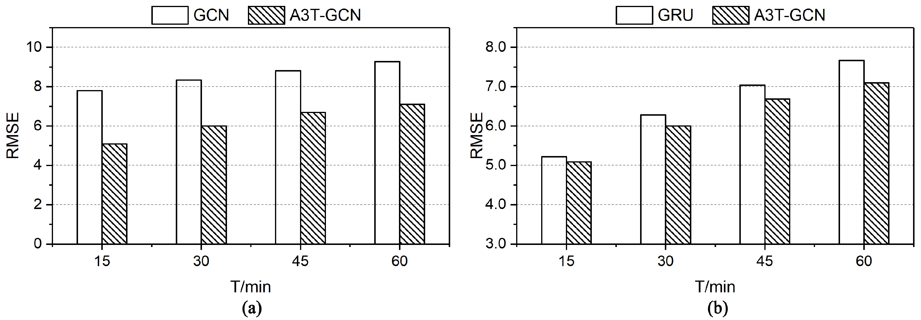
Results based on Los-loop are similar to those based on SZ-taxi. The prediction error of A3T-GCN is kept lower than that of GCN in 15, 30, 45, and 60 min of traffic forecasting, as shown in Figure 3a. A3T-GCN achieves approximately 34.67%, 28.05%, 24.08%, and 23.38% lower RMSEs in 15, 30, 45, and 60 min of traffic forecasting time series, respectively. As for the comparison with GRU shown in Figure 3b, A3T-GCN achieves approximately 2.45% lower RMSE in 15 min traffic forecasting, approximately 4.50% lower RMSE in 30 min traffic forecasting, approximately 4.98% lower RMSE in the 45 min time series, and approximately 7.35% lower RMSE in the 60 min time series.

Figure 2 and Figure 3 show that the A3T-GCN has better prediction capabilities than the GCN and the GRU, respectively. In other words, the A3T-GCN model can capture the spatial topological characteristics of urban road networks and the temporal variation characteristics of the traffic state simultaneously, which means it maintains superiority under various prediction horizons compared with the GRU and the GCN.

3.3.3. Long-Term Prediction Capability

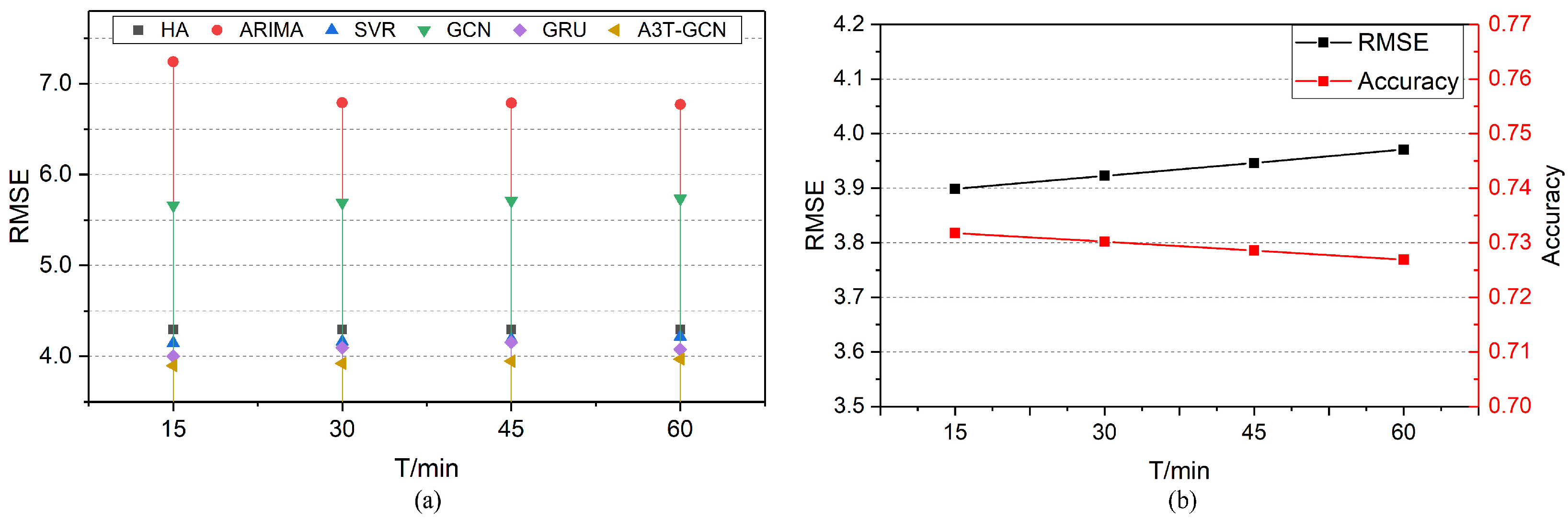
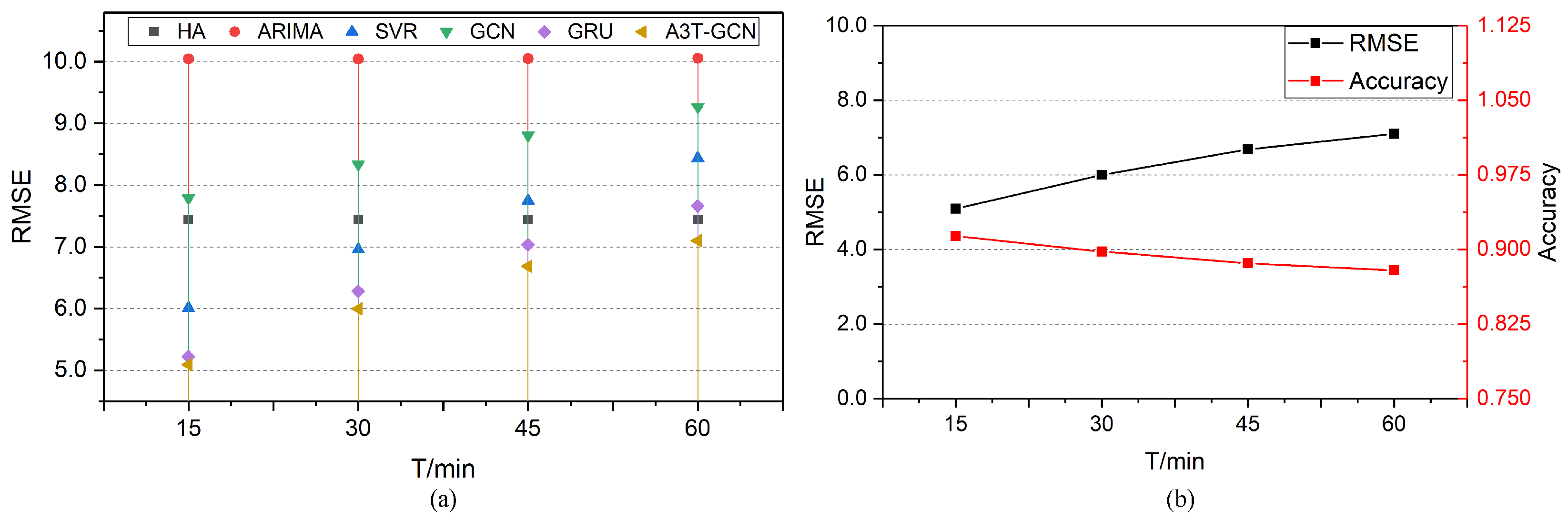
The long-term prediction capability of A3T-GCN was tested for traffic speed forecasting in 15, 30, 45, and 60 min prediction horizons. The RMSE comparison of different models under different prediction horizons is shown in Figure 4a. The RMSE of the A3T-GCN is the lowest under all lengths of time series. The variation trends of RMSE and accuracy, which reflect prediction error and precision, respectively, of the A3T-GCN under different prediction horizons, are shown in Figure 4b. We can observe that the RMSE increases as the length of the time series increases, whereas the accuracy declines; both change slightly and show a certain stability. Compared with GRU (which outperforms other baselines), A3T-GCN has a standard deviation of approximately 0.03 in RMSE, while that of the GRU is approximately 0.06.

The forecasting results based on Los-loop are shown in Figure 5, and consistent laws are found. In sum, A3T-GCN has good long-term prediction capability. It can maintain the best performance under 15, 30, 45, and 60 min prediction horizons, as shown in Figure 5a. Figure 5b shows that the forecasting results of A3T-GCN change slightly with changes in the prediction horizons, thereby showing a certain stability. Compared with GRU (which outperforms other baselines), A3T-GCN has a standard deviation of approximately 0.76 in RMSE, while that of the GRU is approximately 0.91. Therefore, the A3T-GCN is applicable to short-term and long-term traffic forecasting tasks.

3.3.4. Effectiveness of Introducing Attention to Capture Global Variation

A3T-GCN and T-GCN were compared to test the superiority of capturing global variation. The results are shown in

Table 3. Comparison of forecasting results between A3T-GCN and T-GCN under different lengths of time series based on SZ-taxi and Los-loop.

T	Metric	SZ-Taxi		Los-Loop
		T-GCN	A3T-GCN	T-GCN	A3T-GCN
	RMSE	3.9325	3.8989	5.1264	5.0904
	MAE	2.7145	2.6840	3.1802	3.1365
15 min	Accuracy	0.7295	0.7318	0.9127	0.9133
	$R^2$	0.8539	0.8512	0.8634	0.8653
	var	0.8539	0.8512	0.8634	0.8653
	RMSE	3.9740	3.9228	6.0598	5.9974
	MAE	2.7522	2.7038	3.7466	3.6610
30 min	Accuracy	0.7267	0.7302	0.8968	0.8979
	$R^2$	0.8451	0.8493	0.8098	0.8137
	var	0.8451	0.8493	0.8100	0.8137
	RMSE	3.9910	3.9461	6.7065	6.684
	MAE	2.7645	2.7261	4.1158	4.1712
45 min	Accuracy	0.7255	0.7286	0.8857	0.8861
	$R^2$	0.8436	0.8474	0.7679	0.7694
	var	0.8436	0.8474	0.7684	0.7705
	RMSE	4.0099	3.9707	7.2677	7.099
	MAE	2.7860	2.7391	4.6021	4.2343
60 min	Accuracy	0.7242	0.7269	0.8762	0.8790
	$R^2$	0.8421	0.8454	0.7283	0.7407
	var	0.8421	0.8454	0.7290	0.7415

. The A3T-GCN model shows approximately 0.86% lower RMSE and approximately 0.32% higher accuracy than the T-GCN model under the 15 min time series; approximately 1.31% lower RMSE and approximately 0.48% higher accuracy under the 30 min time series; approximately 1.14% lower RMSE and approximately 0.43% higher accuracy under 45 min traffic forecasting; and approximately 0.99% lower RMSE and approximately 0.37% higher accuracy under the 60 min time series.

Hence, the prediction error of A3T-GCN is lower than that of T-GCN, but the accuracy of the former is higher under different horizons of traffic forecasting, thereby proving the global feature capturing capability of the A3T-GCN model.

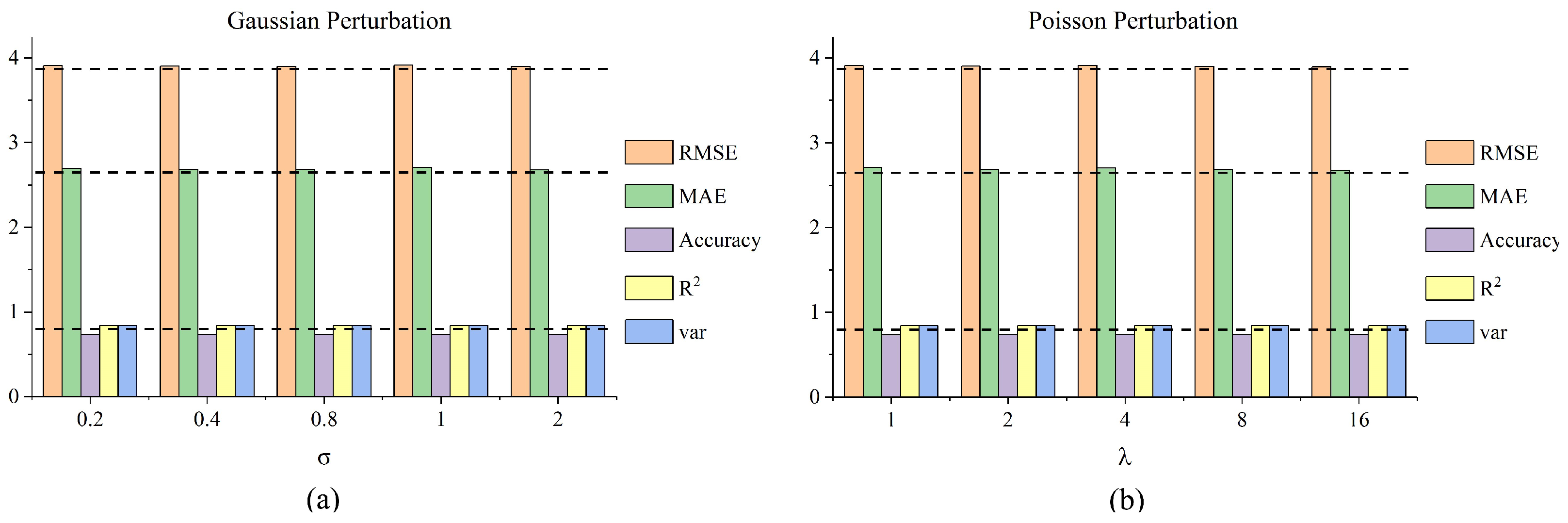
3.4. Perturbation Analysis

Noise is inevitable in real-world datasets. Therefore, perturbation analysis was conducted to test the robustness of A3T-GCN. In this experiment, two types of random noises were added to the traffic data. Random noise obeys the Gaussian distribution $N\in (0,{\sigma }^2)$, where $\sigma \in (0.2,0.4,0.8,1,2)$, and the Poisson distribution $P\left(\lambda \right)$, where $\lambda \in (1,2,4,8,16)$. The noise matrix values were normalized to [0, 1].

The experimental results based on SZ-taxi are shown in Figure 6. The results of adding Gaussian noise are shown in Figure 6a, where the x- and y-axes show the changes in $\sigma$ and in different evaluation metrics, respectively. Different colors represent various metrics. Similarly, the results of adding Poisson noise are shown in Figure 6b. The values of different evaluation metrics remain basically the same regardless of the changes in $\sigma /\lambda$. Hence, the proposed model can, remarkably, resist noise.

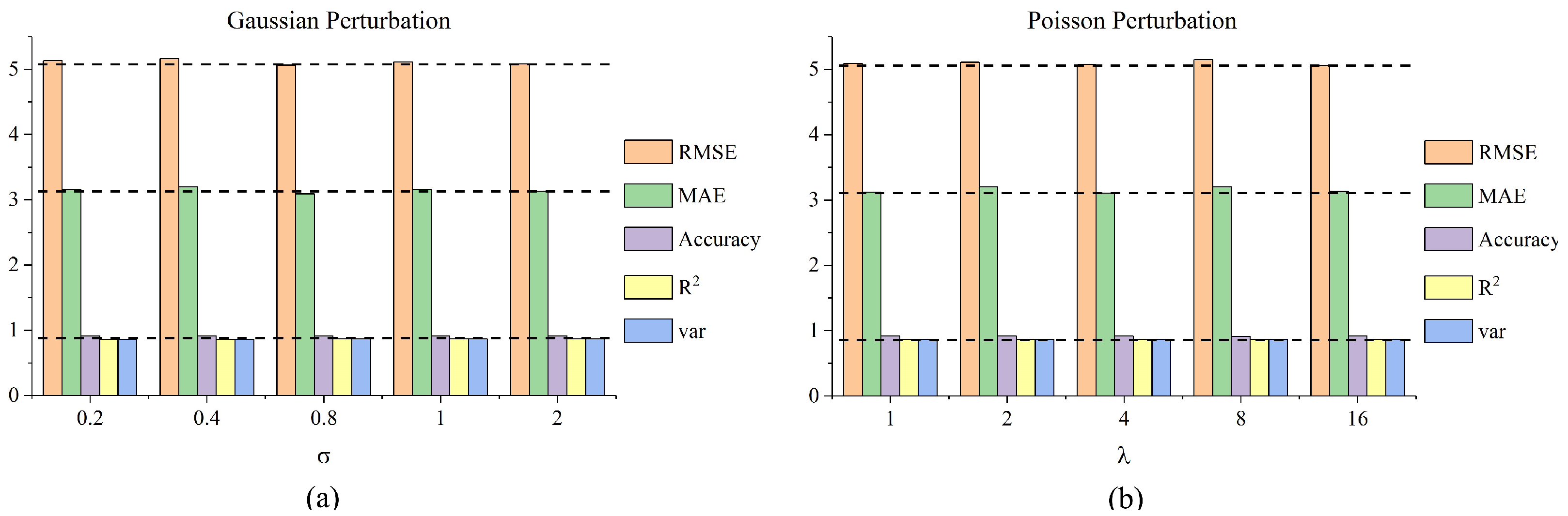
Figure 7a,b indicates that the experimental results based on Los-loop are consistent with the experimental results based on SZ-taxi. Therefore, the A3T-GCN model can remarkably resist noise and still obtain stable forecasting results under Gaussian and Poisson perturbations.

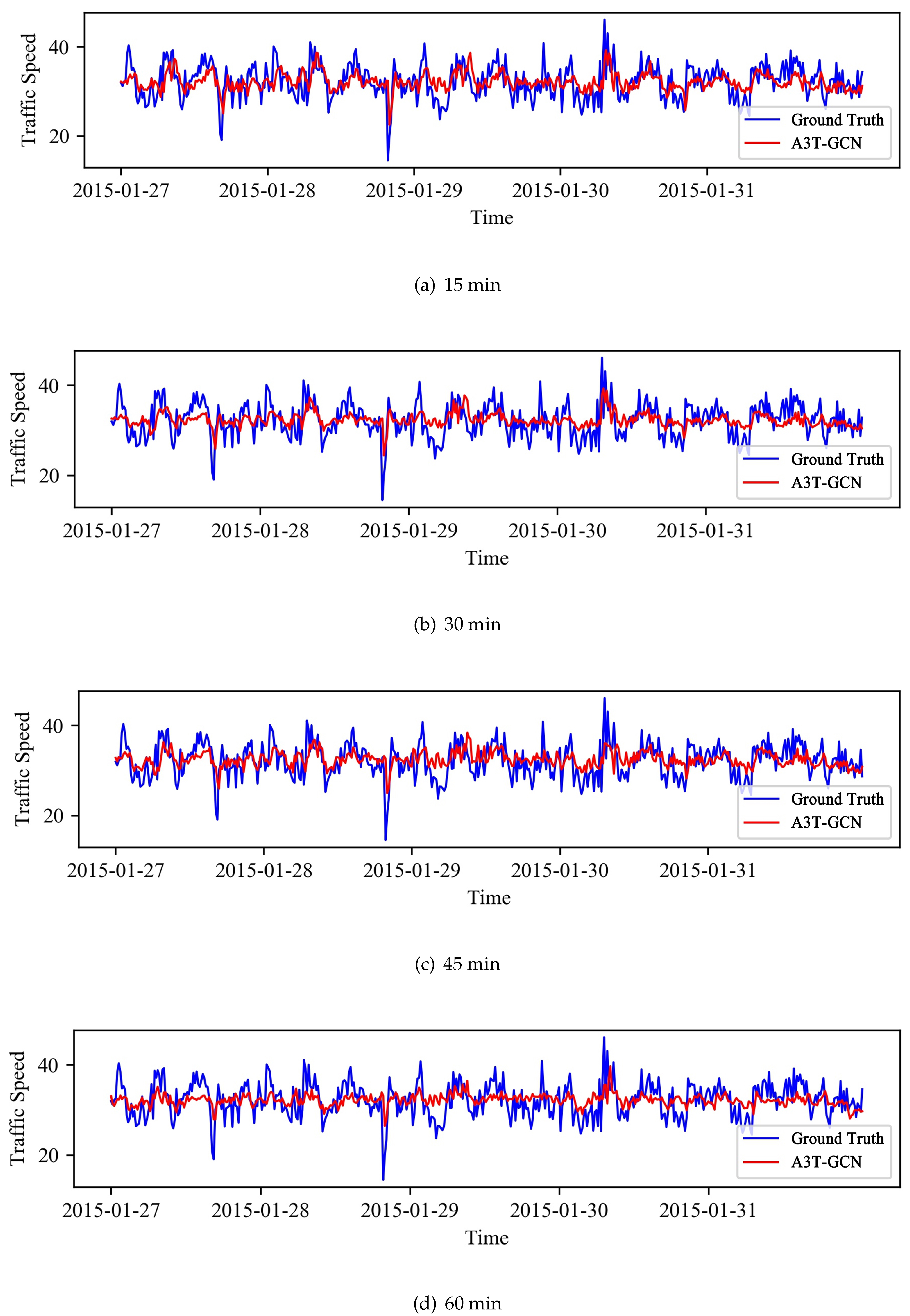
3.5. Visualized Analysis

The forecasting results of the A3T-GCN model based on two real datasets are visualized for a good explanation of the model.

(1) SZ-taxi: We visualize the result of one road on 27 January 2015. Visualization results for the 15, 30, 45, and 60 min time series are shown in Figure 8.

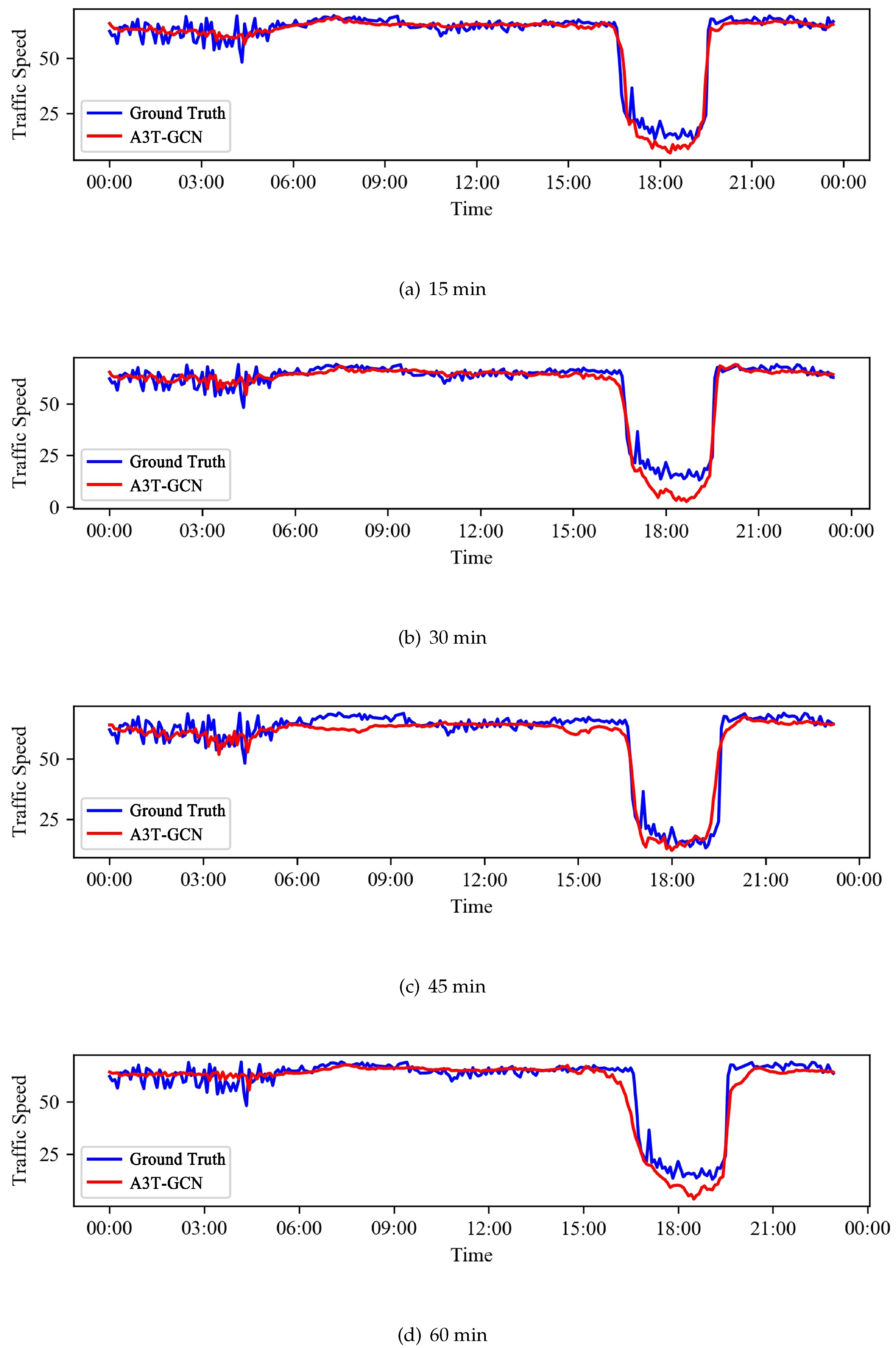
(2) Los-loop: Similarly, we visualize one loop detector data in the Los-loop dataset. Visualization results for the 15, 30, 45, and 60 min are shown in Figure 9.

In sum, the predicted traffic speed shows a similar variation trend to the actual traffic speed under different time series lengths, which suggests that the A3T-GCN model is competent at the traffic forecasting task. This model can also capture the variation trends of traffic speed and recognize the start and end points of rush hours. As suggested by the well-fit of A3T-GCN to the abrupt drops during rush hours in Figure 9, the A3T-GCN model forecasts traffic jams accurately, thereby proving its validity in real-time traffic forecasting.

4. Conclusions

A traffic forecasting method called A3T-GCN is proposed to capture global temporal dynamics and spatial correlations simultaneously and to facilitate traffic forecasting. The urban road network is constructed into a graph, and the traffic speed on the roads is described as attributes of nodes on the graph. In the proposed method, the spatial dependencies are captured by GCN based on the topological characteristics of the road network. Meanwhile, the dynamic variation of the sequential historical traffic speeds is captured by GRU. Moreover, the global temporal variation trend is captured and assembled by the attention mechanism. Finally, the proposed A3T-GCN model is tested on the urban road network-based traffic forecasting task using two real datasets, namely, SZ-taxi and Los-loop. We observe the improvements in RMSE of 2.51–46.15% and 2.45–49.32% over baselines for the SZ-taxi and Los-loop, respectively. Meanwhile, the accuracies are 0.95–89.91% and 0.26–10.37% higher than the baselines for the SZ-taxi and Los-loop, respectively. The results show that the A3T-GCN model is superior to HA, ARIMA, SVR, GCN, GRU, and T-GCN in terms of prediction precision under different lengths of prediction horizon, thereby proving its validity for real-time traffic forecasting.