
Semantic Relation Model and Dataset for Remote Sensing Scene Understanding


1
School of Computer and Communication Engineering, University of Science and Technology Beijing, Beijing 100083, China
2
Beijing Key Laboratory of Knowledge Engineering for Materials Science, Beijing 100083, China
3
Surgery Simulation Research Laboratory, University of Alberta, Edmonton, AB T6G 2E1, Canada
4
FINTECH Innovation Division, Postal Savings Bank of China, Beijing 100808, China
*
Author to whom correspondence should be addressed.
ISPRS Int. J. Geo-Inf. 2021, 10(7), 488; https://0-doi-org.brum.beds.ac.uk/10.3390/ijgi10070488
Submission received: 4 May 2021
/
Revised: 22 June 2021
/
Accepted: 9 July 2021
/
Published: 17 July 2021
(This article belongs to the Special Issue Deep Learning and Computer Vision for GeoInformation Sciences)
Abstract
:A deep understanding of our visual world is more than an isolated perception on a series of objects, and the relationships between them also contain rich semantic information. Especially for those satellite remote sensing images, the span is so large that the various objects are always of different sizes and complex spatial compositions. Therefore, the recognition of semantic relations is conducive to strengthen the understanding of remote sensing scenes. In this paper, we propose a novel multi-scale semantic fusion network (MSFN). In this framework, dilated convolution is introduced into a graph convolutional network (GCN) based on an attentional mechanism to fuse and refine multi-scale semantic context, which is crucial to strengthen the cognitive ability of our model Besides, based on the mapping between visual features and semantic embeddings, we design a sparse relationship extraction module to remove meaningless connections among entities and improve the efficiency of scene graph generation. Meanwhile, to further promote the research of scene understanding in remote sensing field, this paper also proposes a remote sensing scene graph dataset (RSSGD). We carry out extensive experiments and the results show that our model significantly outperforms previous methods on scene graph generation. In addition, RSSGD effectively bridges the huge semantic gap between low-level perception and high-level cognition of remote sensing images.
1. Introduction
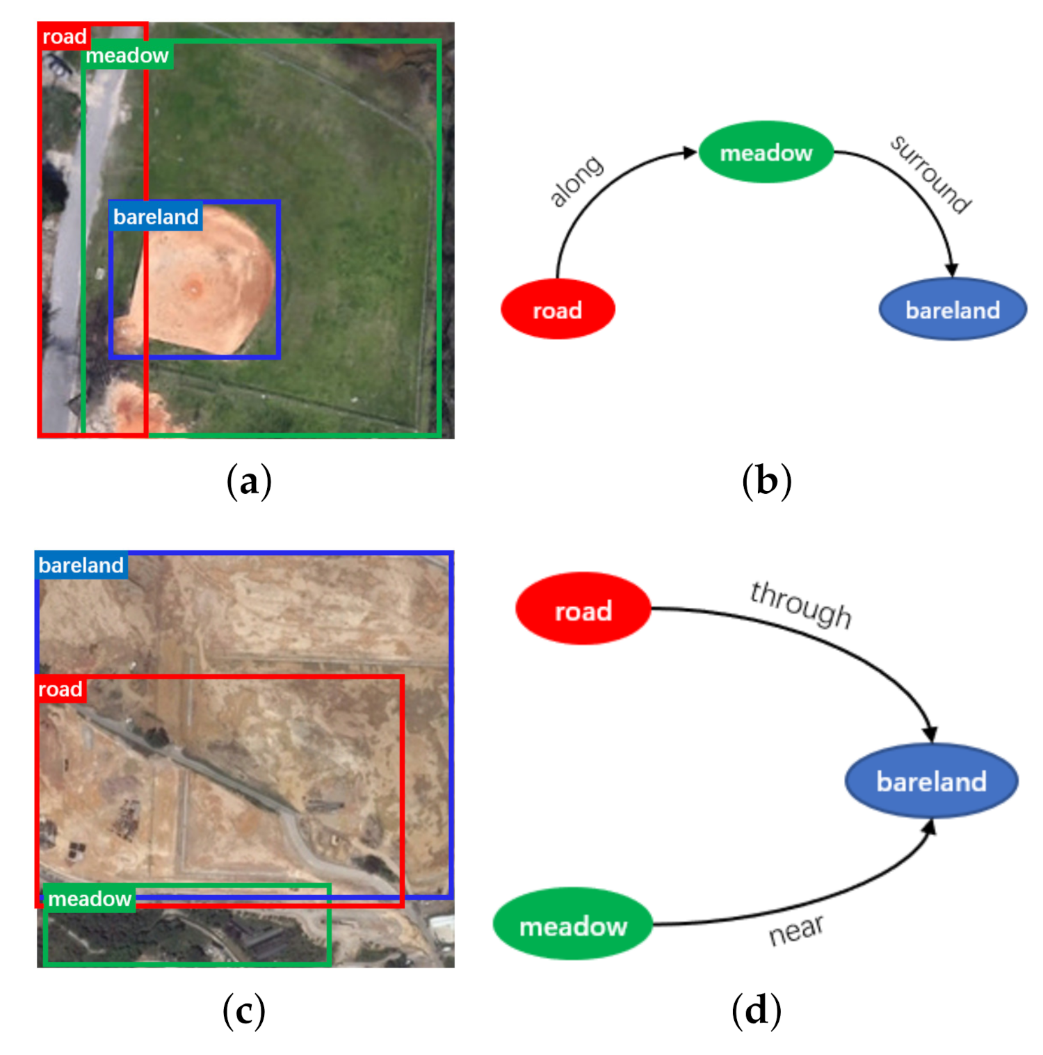
With the rapid development of space exploration technology, plentiful high-resolution remote sensing images have been accumulated, which provides a solid data support for in-depth understanding of remote sensing scenes [1,2,3,4]. Existing remote sensing image processing technologies mainly focus on perception-level tasks such as classification [5], object detection [6,7] and semantic segmentation [8,9]. In particular, with the breakthrough of artificial intelligence (AI) techniques represented by deep learning, the accuracy of category recognition has been qualitatively improved no matter in image-level or pixel-level [10]. However, to understand a remote sensing scene thoroughly, it is not enough to stay at perceptual level. As shown in Figure 1a,c, object detection cannot distinguish the essential differences between baseballfield and desert, which contain the same categories (e.g., “road”, “bareland”, “meadow”). The main reason is these models are blind to the spatial relations between entities [11]. In order to obtain the rich semantic relations from image scene, many researchers have conducted a series of valuable studies [12,13,14]. One of the most effective methods is to express the visual scene as a structured graph [15]. In this kind of graphs, semantic interaction between nodes (including subject and object) can be represented in a form like . In summary, semantic relationship reasoning involves detecting and localizing pairs of nodes in an image, meanwhile, classifying the interactive relationship of each pair. Therefore, the semantic differences among baseballfield and desert can be clearly identified based on the analyses from Figure 1b,d, it is obvious that baseballfield usually contains relationship , different with in desert. As a result, the scene graph serves as a natural link between the low-level perceptual tasks (e.g., image classification, object detection) and the high-level cognitive tasks such as image caption [16,17], visual question answering [18] and image retrieval [19].
Scene graph generation has become the preoccupant relation reasoning method in the field of nature images and obtained numerous achievements [20,21,22]. However, the relevant research is rare and the progress is relatively slow in remote sensing. Due to the obvious diversities between natural images and remote sensing images, the direct transfer from existing models to remote sensing is often ineffective [23]. Concerning various sizes, aspect ratios and sparse spatial distribution of ground objects in remote sensing images, we introduce dilated convolution [24] into attentional graph convolution network to construct a multi-scale semantic fusion scheme for remote sensing relationship reasoning. By adjusting the cognitive receptive field, our model is guided to pay attention to the context information corresponding to different semantic ranges, and the semantic content can be effectively integrated through a particular message passing mechanism.
In terms of semantic cognition dataset, researchers [25,26] began to pay more attention to the scene understanding of remote sensing in recent years. Among them, Lu et al. [23] proposed the largest dataset for captioning remote sensing image—RSICD, which has high intra-class diversity and low inter-class dissimilarity. According to the statistical analysis, this dataset contains 10,921 remote sensing images with a size of 224 × 224, 24,333 different descriptive sentences made up of 3323 words, and each image corresponds to five sentences. RSICD [23] has become the universal dataset of remote sensing image caption task and been widely applied [27].
However, RSICD [23] only contains descriptive statements without additional and meaningful annotations about the various entities in remote sensing images, such as labels, region bounding boxes, attributes and relationships, which play an indispensable role in exploring scene representations comprehensively. In particular, based on these information, we can construct remote sensing scene graph, which forms a connecting link between visual feature extraction tasks [5,6,7] and high-level semantic cognition tasks [26,28]. Therefore, a remote sensing scene graph dataset is proposed to further improve the development of semantic relationship cognition in remote sensing field.
In summary, the main contributions of this paper include four aspects:
- To deal with the inherent characteristics in remote sensing images, such as large spans and particular spatial distribution of entities, this paper introduces dilated convolution [24] into our method and builds a multi-scale graph convolutional network creatively, which is helpful to expand the cognitive vision of semantic information.
- A novel multi-scale semantic fusion network is presented for scene graph generation. In addition, to improve the efficiency of relation reasoning, translation embedding (TransE) [29] is adopted to calculate the correlation scores between nodes and further eliminate the invalid candidate edges.
- Aiming at the construction task of remote sensing scene graph, a tailored dataset is proposed to break down the semantic barrier between category perception and relation cognition. To the best of our knowledge, RSSGD is the first scene graph dataset in remote sensing field.
2. Related Works
2.1. Scene Graph Generation
In fact, the idea of using contextual semantic content to improve scene understanding has been studied for a long time [30,31,32,33]. In recent years, inspired by a series of fruitful studies in computer vision tasks [34,35], Johnson et al. [19] proposed an issue of extracting scene graph from image, and extended object detection [36] to the cognitive task of inferring semantic relations. Schuster et al. [37] proposed a model for scene graph generation including two modules: a rule-based network and a classifier-based network, which map dependency syntax representations into scene graph. Inspired by the advances of TransE [29] in relational reasoning, some relevant models are constructed for visual relationship recognition [38,39]. These TransE-based methods place the semantic information in a low-dimensional mapping space, where the relations are represented as valuable translation vectors. Many previous works focus on building a scene graph from an input image but neglect the surrounding context, as a result, these local predictions are often isolated each other. However, the scene graph generation based on context information can solve the above ambiguity problem. Inspired by this, Xu et al. [40] proposed a model by applying iterative message passing to extract scene relationships. Hu et al. [41] integrated three attentional graph structures to decompose the prefixal expression into subject, relation and object, respectively, and introduced modular neural framework to match the extracted context symbols with image regions. Zellers et al. [42] find that some inherent relational patterns exist even in larger subgraphs, and more than half of images contain these substructures that frequently occurred before. Based on the above analysis, a neural network structure called Motifs has been proposed. Motifs [42] builds a new global context computing mechanism and allocates labels to the interactive relations between nodes by combining head, tail, and joint boundary region information with an outer product. A multi-level scene description network (MSDN) [43] integrate object detection, scene graph generation and image caption into a unified model to achieve a comprehensive understanding of image, and the mainly operation of MSDN [43] is to pass and update context information among three visual tasks by constructing dynamic subgraphs. A pre-trained tensor-based relational module [44] is used as the prior domain knowledge to refine the relationship reasoning, moreover, a message passing scheme with gated recurrent units (GRU) is introduced to improve the accuracy of semantic relation detection. Herzig et al. [45] proposed a scene graph predictor to reinforce relationship representation by exploring the interdependencies between nodes and relationships. To improve the final performance of scene graph generation, Lu et al. [15] trained a feature extraction module and a language priors module, respectively, and then combined them together through an objective function. Yu et al. [46] adopt the prior knowledge of linguistic statistics to normalize visual feature learning and reduce the cost of model training. A context-dependent diffusion network [47] learned semantic knowledge through a word graph and obtained spatial representation by extracting the low-level features, then these two types of global context information were adaptively merged by a diffusion network to deduce the potential semantic relationships.
2.2. Scene Graph Dataset
Johnson et al. [19] proposed a real-world scene graph dataset (RW-SGD), which is the first dataset explicitly created for scene graph generation. RW-SGD [19] is constructed by gathering 5000 images from Microsoft COCO [48], and using Amazon’s Mechanical Turk to produce human-generated scene graphs corresponding to these selected images. VRD [15] is built for the task of semantic relationship inference, which has 100 object classes extracted from 5000 images and contains 37,993 relationships. However, the distribution of these interactive relationships in VRD [15] has a common problem of long tail in scene graph datasets. Visual Genome (VG) [49] is a large-scaled relation dataset, which consists of many components, such as attributes, relationships, question answer pairs. At present, VG [49] has widely been applied to scene graph generation, image caption and visual question answering for its huge number of images and relationships. In addition, another scene graph dataset VrR-VG [50] is generated based on VG [49]. UnRel-D [51] is a new challenging dataset of unusual relations including more than 1000 images, which can be queried with 76 triplet queries.
2.3. Attention Mechanism
In remote sensing field, Haut et al. [52] proposed a residual channel attention-based network which integrated the attention module into residual convolutional neural network (CNN) layers. Luo et al. [53] introduced channel attention mechanism into fully convolutional network (FCN) to select appropriate features. Wang et al. [54] improved FCN by adopting a class-specific attention model. Ba et al. [55] incorporated spatial and channel-wise attention networks in CNN architectures to enhance features and detect fire smoke from satellite pictures. In order to deal with the semantic segmentation task of remote sensing images, Li et al. [56] proposed a dual path attention network, designing a spatial attention module to extract pixel-level spatial context and introducing a channel-wise attention module to exploit key local features in different regions.
2.4. Graph Convolutional Network
Because of the excellent ability to capture spatial features, CNN has been applied in many vision tasks [5,53,55]. However, most CNN models are weak in modeling relations between objects. For breaking through the limitations of grid sampling, graph convolutional network [57] has been proposed and successfully applied in irregular or non-grid data representation and analysis recently [58]. For instance, to accurately forecast urban traffic based on digital road map, Zhao et al. [59] proposed a temporal graph convolutional network (T-GCN), which is composed of a graph convolutional network and a gated recurrent unit. In T-CGN [59], the GCN is used to learn multi-level semantic representation for obtaining spatial information and the gated recurrent unit is used to learn dynamic changes of traffic data for capturing temporal context.
There are a few works related to GCN in remote sensing field. Shahraki et al. [60] proposed a cascaded GCN for hyperspectral image classification. Qin et al. [61] extended the original GCN to a second-order version by simultaneously considering spatial and spectral neighborhoods. Wan et al. [62] performed super-pixel segmentation on remote sensing images and fed the results into GCN to reduce the computational cost for improving the recognition efficiency. Based on a specific graph structure, Mou et al. [63] presented a novel convolution operator and combined it with a neural network to construct a new learning model for analyzing unstructured spatial vector data. In order to extract discriminative features from irregular structures, Khan et al. [64] proposed a novel multi-label scene recognition technique for remote sensing image classification using deep GCN. Shi et al. [65] integrated GCN and deep structured feature embedding (DSFE) into an end-to-end framework. Furthermore, instead of adopting a classic GCN, DSFF [65] used a gated graph convolutional network, which can generate clear boundary and process fine-grained pixel-level recognition in remote sensing by refining weak and coarse semantic prediction. In this paper, GCN is mainly used for information passing and fusion across the scene graph of remote sensing images, as well as the renewal of a node state.
3. Materials and Methods
3.1. Scene Graph Generation Model for Remote Sensing Image
In the field of semantic scene cognition, researchers have carried out some preliminary studies in remote sensing field and obtained many exciting achievements. However, if a model crosses from the low-level feature perception to the high-level scene understanding directly, but lacks the necessary support from semantic relationships between entities, it will mechanically overfit the labeled data and fail to truly understand the remote sensing scenes. For instance, Lu et al. [23] pointed out just because of the high co-occurrence between “tree” and “building”, even though an image contains tree but no building, the label "building" often appears in the recognition result.
Scene graph is a topological representation, which encodes the objects and their relationships of a visual scene. In short, the task of scene graph generation is to construct a graphical structure whose nodes and edges are related to the entities and relations from input image, so as to deepen the understanding about a scene rather than just treating an image as a collection of objects separated from each other [66].
From the perspective of scene graph G, an image I is composed of node set B and edge set E, where these relational nodes semantically correspond to the subject S and object O of triplet, respectively. Furthermore, R is formed by the semantic relations labeled with the interactive predicates between subjects and objects. Therefore, the generation of scene graph can be described as follows:
Unlike Graph R-CNN [66], we introduce TransE [29] to calculate the relation scores between nodes in visual scenes for pruning the meaningless connections. Besides, considering the drastic changes of entity scale and aspect ratio in remote sensing field, the mechanism of dilated convolution is introduced into graph convolution model to refine and broadcast the semantic information of remote sensing scenes at different scales. The framework proposed in this paper can thoroughly integrate the acquired semantic content, and further predict the potential semantic relationships between nodes effectively. As a result, our method is naturally suitable for remote sensing image understanding.
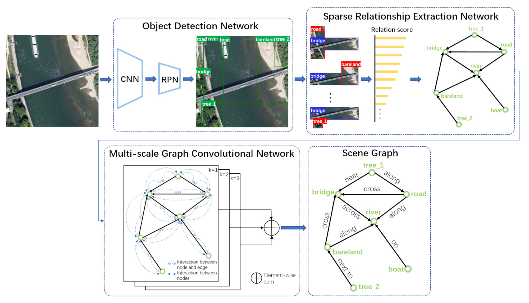
There are three sub-modules in our MSFN as shown in Figure 2.
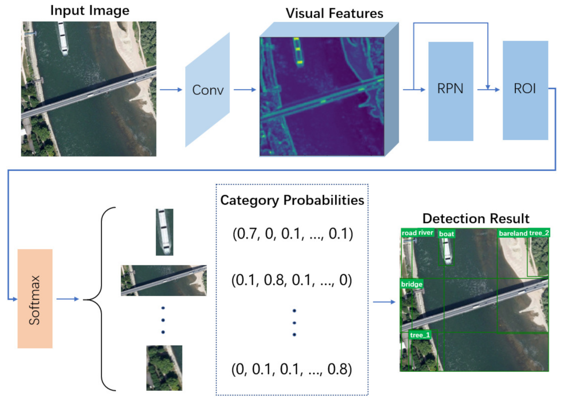
- Object Detection Network. The target patches with their initial categories are identified by this detection framework from the input pictures. In general, the regions are marked by a group of bounding boxes one by one. The details are shown in Figure 3.
- Sparse Relationship Extraction Network (SREN). This module is designed for calculating and sorting the scores of relations between all pairs of nodes (red box representing subject and blue box representing object) to remove the invalid or weak correlation node pairs, so as to clarify the semantic combinations of subjects and objects.
- Multi-scale Graph Convolutional Network (MS-GCN). Based on the selected node pairs with strong semantic relatedness, the multi-scale contextual information in visual scene is propagated and fused to infer the categories of relationships, and a scene graph is finally generated.
3.1.1. Object Detection Network
For the fair comparison with existing classical methods [39,42,66], this paper adopts the general object detection architecture [35] to identify entities and extract visual features. From Figure 3 we can find, for each image I, a group of feature maps are first extracted by the convolutional operations in backbone network, whose framework is described in Table 1. Then based on the extracted features, the region proposal network (RPN) and region of interest (ROI) pooling predict a set of bounding boxes , C is the number of entities contained in I. Finally, all bounding boxes are classified by Softmax. For each proposal , it corresponds to a feature vector and a probability vector of initial node label, and Y is the number of categories.
Figure 3.
The overview of object detection network.

It should be noted that these initial node categories predicted by object detection network are mainly used for screening the potential relationships in Section 3.1.2, and the final node labels will be determined through multi-scale context interaction and fusion in Section 3.1.3. In addition, will be applied to the subsequent refinement of multi-scale semantic information.
3.1.2. Sparse Relationship Extraction Network
Although remote sensing images usually have large scale and complex spatial structure [67], not all entities are related to each other, and the relationships between them are sparse in general [66]. In addition, if an image includes C entities, then candidate node pairs will be generated. Moreover, remote sensing images often contain lots of ground objects, if the relations of all pairs are predicted, the computing cost will be undoubtedly huge.
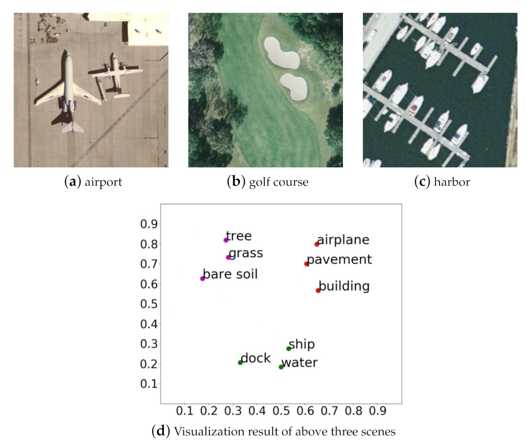
It can be vividly demonstrated in Figure 4 that if entities belong to a special semantic scene (e.g., “airport”, “golf course”, “harbor”), they will flock together, otherwise, they stay away from each other (e.g., “airplane”, “ship”). In addition, the nodes with underlying semantic relationships in the same scene will get much closer, such as “tree” and “grass”, “airplane” and “pavement”, “ship” and “water”. Based on the above analysis, we first calculate the node relation scores in visual scene, then rank these scores in descending order, and select the top 70 percent of all pairs as the candidate relationships finally. The aim of doing this is to trim out invalid edges and weaken their interferences in the cognition of valuable semantic relationships, which is crucial to improve the efficiency and accuracy of scene generation construction.
The computational process of semantic relation score can be defined as:
where is a nonlinear function; , and are the visual features of subject, object and relationship (union of subject and object); , and are the transformation matrixes to be learned, respectively.
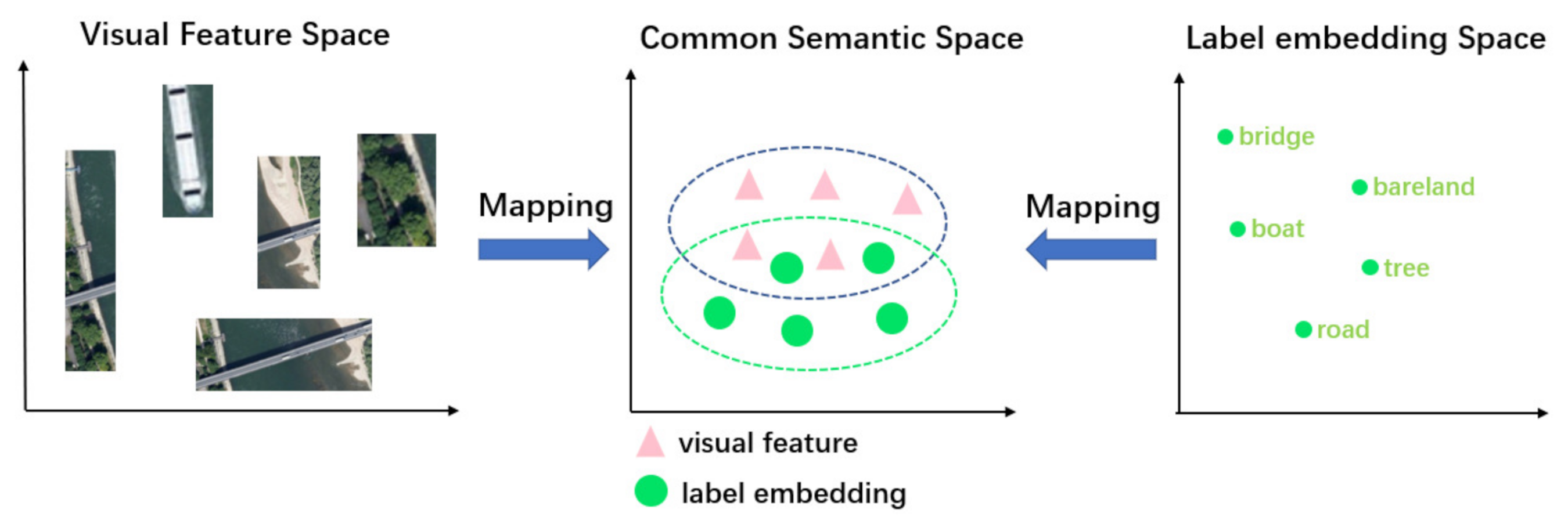
Inspired by the translation between visual features and semantic relations in VTransE [39], we map the visual features and semantic embeddings of nodes into a potential space as shown in Figure 5, and the mapping constraint is carried out by Equation (3), which is beneficial to measure the semantic relation scores more accurately.
where , are the label embedding representations of subject and object, respectively, denotes loss.
3.1.3. Multi-Scale Graph Convolutional Network
Due to the obvious diversity of entity size and spatial distribution in remote sensing field, the ground objects may present different semantics given a series of cognitive scales in remote sensing scene [67,69].
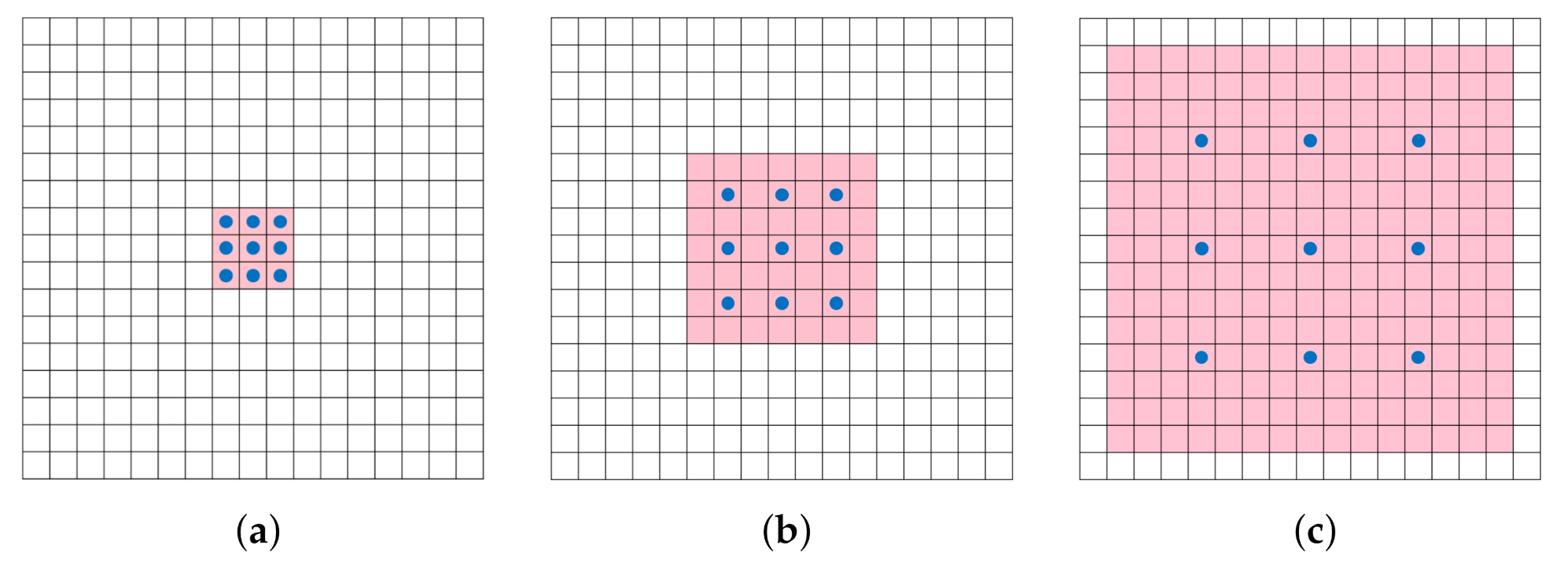
From Figure 6 we can find that with the increase of dilated rate, which refers to the distance between two adjacent neurons of convolution kernel, the receptive field grows exponentially. Furthermore, dilated convolution [24] will turn into traditional convolution when dilated rate equals 1. Experimental results show that fusing multi-scale context information by adopting dilated convolution [24] can observably improve the accuracy of semantic segmentation tasks without significantly increasing the number of parameters and the cost of computation [70]. The reason behind this is the special convolution expands the receptive field without losing resolution [71].
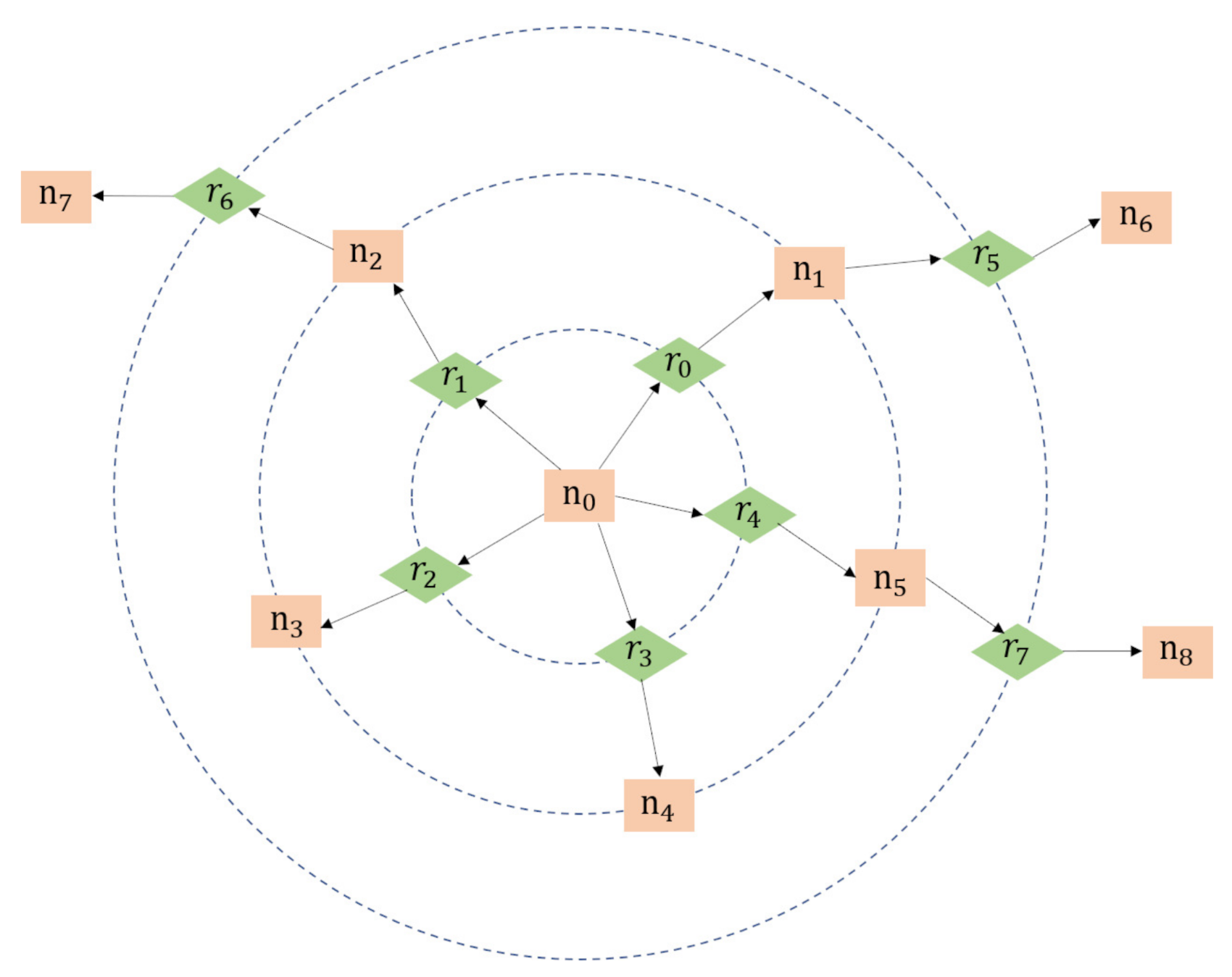
Based on the above analyses, we believe that dilation operation can also contribute to adjusting the receptive field of semantic context. Therefore, a novel multi-scale graph convolutional network is proposed in this paper by introducing dilated convolution [24]. In this structure, the semantic contexts from different levels are interacted by setting corresponding dilated rates, which is the key to expanding the cognitive view of our model and strengthening its ability to understand remote sensing scenes. In this paper, we aggregate neighbors in different cognitive levels by matching dilated rate with the skipped distance between nodes, and the specific operation is demonstrated in Figure 7.
As shown in Figure 7, in the first level, the edge set interacting with node is , and the node set related to is . In the second level, the edge set associated with is , and the node set interacting with is . Similarly, in the first level, the node set connecting with edge is . In the second level, the node set interacting with is .
In computer vision tasks, one important issue is to extract visual features and classify them. Due to the entities in large remote sensing pictures are always distributed unevenly and easily confused with each other, so the above research is more crucial in remote sensing image processing. Recently, deep learning-based attention mechanism [72] is regarded as an excellent solution by perceiving object-level features to illustrate the main sematic information in remote sensing scenes. For instance, [21] used a neural network with self-attention mechanism to embed context via constructing an adjacency matrix based on the space positions of entities. An attention graph network [73], an attention graph network is proposed to generate scene graph directly from the top layer of a pre-trained transformer, from which model can obtain the feature information and graph node connectivity simultaneously.
However, due to the complex presentation of remote sensing scene, traditional attention methods usually become insensitive to some inconspicuous but meaningful entities in processing remote sensing images [27]. Therefore, it is necessary to integrate local and global information for improving recognition precision. In this paper, the attention mechanism allocates corresponding weights to different regions of image, and leads model to focus on the context information in specific semantic range.
In order to guide our approach to concentrate fully on the semantic context at the particular level k, (K is the maximum dilated rate), we introduce attentional mechanism to make the network adaptively recognize the information from neighboring nodes and relations. The node’s attentional weight associated with the node is expressed as:
where is the neighboring set of the node at level k. and are the ReLU non-linear activation and concatenation operation, respectively, A refers to the attentional parameters of a single-layer feedforward neural network, is a weight matrix to be learned.
A graph convolutional network [74] for scene understanding is constructed to jointly detect the entity properties and relational semantics. In this method, to effectively represent semantic relations, a visual encoder is designed to produce distinguishable and type-aware relationship embeddings, which are constrained by both the language priors and context information. Given the sparse connectivity of scene graph, an attentional graph convolution network (AGCN) [66] is implemented to optimize visual features and relationship representations among neighbors by passing semantic context throughout a graph structure.
In terms of the interaction and fusion of semantic information at different levels, we also use GCN to update the node context and relation context iteratively, and the specific refining process is described as follows:
where is the neighboring node set of node i at the level, is the number of node set. is the neighboring relation set of node i at the level, and is the number of elements. and are the mapping parameters to be learned. is initialized by the original visual feature when step . is a nonlinear function.
where is the neighboring node set of relation r at the level, and is the number of this set. is initialized by the original visual feature of relation r when step , namely, the visual feature of union region between subject and object that r corresponding to.
The predicted label of semantic relationship is formulated by the following equation:
where are the context information of subject and object with potential semantic relation screened out by sparse relationship extraction network, and is the relation context. is a multi-layer perceptron.
In this stage, the cross-entropy loss function is used to optimize the relation reasoning process:
where is the ground-truth label of relationship r. S and O are the subject set and object set associated with the input image.
The predicted node label can be shown as:
where and are the visual feature and semantic context of node i, respectively. is a multi-layer perceptron.
Similarly, the cross-entropy loss function is applied to optimize the prediction process of node label:
where is the ground-truth label of node i, and C is the number of entities contained in image I.
The overall loss function of our method can be described as follows:
where and are the hyper-parameters.
3.2. Scene Graph Dataset for Remote Sensing Image
The long-term purpose of computer vision is to develop a series of models, which can recognize the visual information within a scene intuitively and further deduce the invisible semantic clues shrewdly from the visual context. In terms of current AI techniques, the performance of relevant model still depends on the knowledge learned from annotated dataset heavily. The increasing availability of large amounts of data drives the development of intelligent systems, which underpins the advances in image scene understanding. Moreover, in order to deepen the model’s inference ability to the visual world, it is necessary to supplement its capacities of object detection and interaction reasoning with the experience of human cognition [49]. Large-scale labeled dataset for specific tasks is the key to building computer vision network. However, in the field of remote sensing, there is still no available scene graph dataset. If an existing model is transferred from the original dataset to another one without familiar surrounding context, its performance will degrade dramatically or even fail to work [23].
According to the above analyses, in order to improve the research about remote sensing scene understanding and open up the channel between feature perception and relation cognition, a scene graph dataset for the remote sensing image—RSSGD—is presented in this paper based on the sentences in RSICD [23]. RSSGD is composed of node labels (e.g., “meadow”, “road”), attributes (e.g., “large”, “green”) contained in the original descriptive content, region coordinates and the relationships (e.g., “next to”, “has”, “in”) between nodes.
RSSGD provides a multi-level learning platform for remote sensing images. In other words, this dataset supports multidimensional studies in computer vision. By enhancing the detectability to nodes and promoting the cognitive level on interactive relationships, the models trained on RSSGD will obtain a more systematic understanding of remote sensing scenes.
The detailed construction rules are described as follows:
- If there is more than one description of relationship in the same node pair, the one most consistent with the actual image scene or with the highest occurrence frequency will be chosen.
- The label should be in the singular form. However, for multiple descriptions, such as “some planes”, the solution is: “some” denotes attribute and “plane” denotes label. Similarly, “two cars” is treated as two nodes labeled with “car”, which can be distinguished by “car_1” and “car_2” in visual representation.
- To maintain the universality and expansibility of annotations, if the labels of the same kind of entities are divergent, the one most consistent with the actual image content or with the highest occurrence frequency shall prevail. For example, “office building” and “business building” are collectively called “building”, and “airport runway” is expressed as “runway”.
RSSGD is a remote sensing scene graph dataset built on the descriptive sentences of RSICD. However, in addition to these descriptive statements, RSSGD also considers adequately the practical semantic scenes of images during the construction process. Therefore, the numbers of entities and categories in the two datasets are not matched strictly. Futhermore, in order to prevent the trained models from over-fitting high-frequency relationships, we always deliberately mine those uncommon relationships with profound cognitive value for a particular scene. RSSGD aims to eliminate the semantic blank between perception and cognition, and support the research of remote sensing scene understanding.
3.2.1. Statistics and Analysis
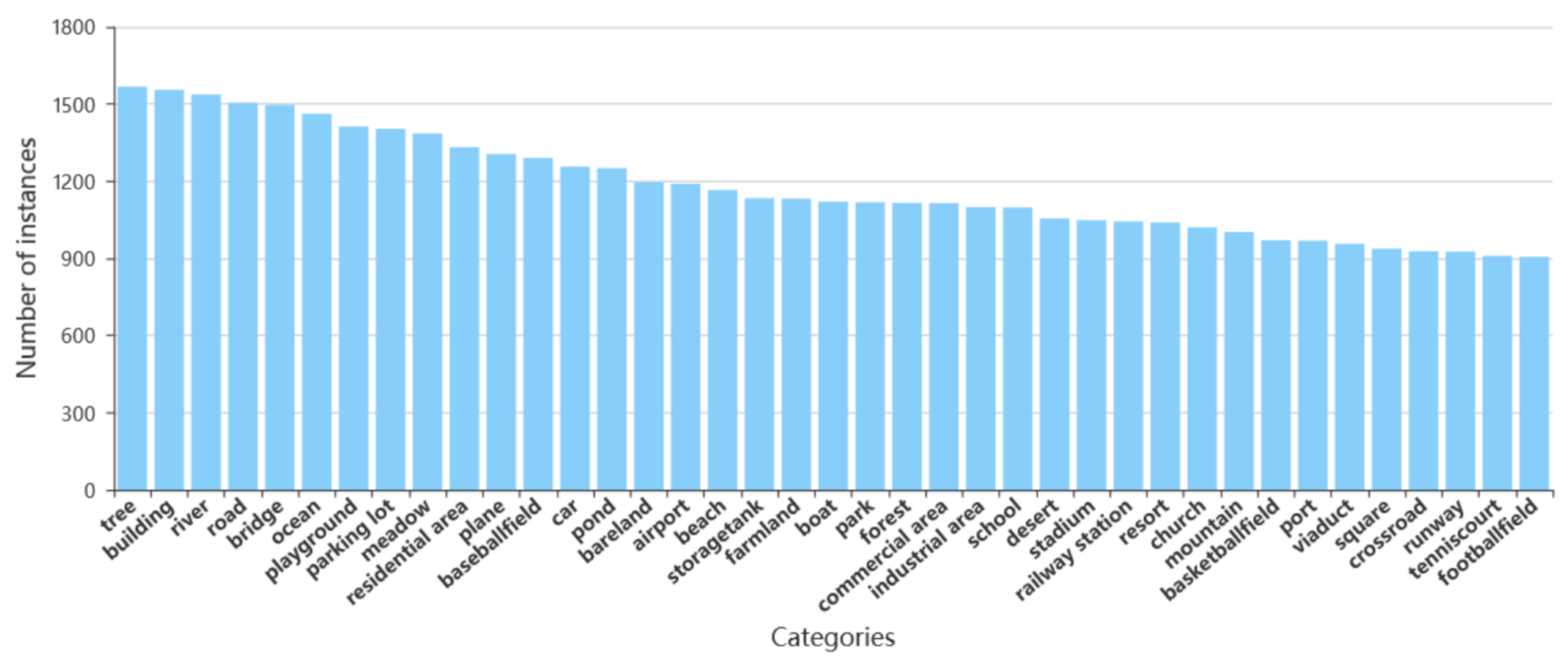
In this section, we provide statistical insights and analysis for our proposed dataset—RSSGD. Specifically, we first break up a scene graph into three constituents—categories, attributes and relations—and then study the number or percentage distribution of each part individually. Based on these statistical results, we can accurately analyse whether our dataset cover usual entities and the necessary relationships between them. In addition, we can also clearly observe whether the fluctuation of distribution is excessive. If these statistical results do not live up to expectations, we will take appropriate measures to optimize RSSGD, such as exploring the missing categories from remote sensing images as much as possible. Furthermore, by purposeful data enhancement we can increase the number of low frequency objects so that the quantitative differences between high frequency categories and low frequency categories are controlled in a moderate range.
From Figure 8 and Figure 9, it can be readily found that RSSGD covers the usual categories (e.g., “tree”, “building”, “road”), attributes (e.g., “green”, “long”, “blue”) and relationships (e.g., “surround”, “in”, “next to”) in remote sensing images. In addition, the percentage distribution is relatively balanced without drastic fluctuations, and the max gap is less than 4% as shown in Figure 9. Therefore, the models trained on RSSGD can treat the high-frequency relationships (e.g., “near”, “on”) and the low-frequency relationships (e.g., “along”, “cover”) equally without discrimination. The purpose behind this is to reduce the model’s biased performance, which is caused by the huge quantitative differences between relations [75].
Specifically, in order to improve the model’s ability to identify entities, we pay more attention to distinguishable information such as shape and color. Affected by the basic hues of actual landforms and satellite remote sensing images, the numbers of “green” and “white” are relatively large, followed by that of “grey”, and “red” has the least instances, which is basically consistent with the real situation. In terms of relationships, to gain a deeper understanding of remote sensing scenes, we focus more on the interactions (as “surround” and “through”) between entities. Because the direction information from remote sensing image is always not clear [23], we have not defined those relationships that representing orientation (e.g., left, right).
3.2.2. Visual Representation
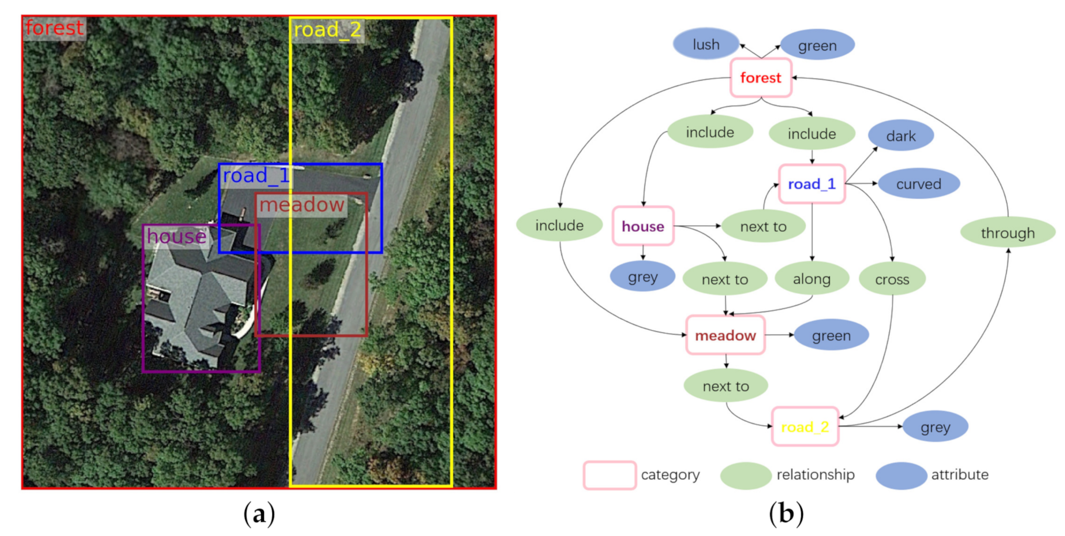
Combining the categories, region boxes, attributes, and relationships associated with entities in one remote sensing picture, we can create a directed graph representation for scene understanding as shown in Figure 10b, which is a structured presentation of the image in Figure 10a. The links connecting two nodes in Figure 10b always start from one subject and end with the related object. In the line linking 2 entities (subject and object), there is a semanic relationship like “include”, “next to” corresponding to it. The attributes are also connected to entities in the graph, as the blue ovals in Figure 10b. With the pictures and corresponding graphs, our RSSGD can be utilized not only for the training of those classification and detection models, but also for scene graph generation algorithms.
In addition, RSSGD can also improve the research on region description due to these relatively fine annotations, such as bounding box, relationship, attribute, etc. For instance, from Figure 10b we can readily obtain two region expressions (“the house is grey” and “the meadow is green”), and the more abundant semantic information (“the grey house is next to the green meadow”) can be gained by connecting them through their interactive relation (“next to”).
In summary, this work pushes toward a more comprehensive understanding of remote sensing images by constructing a scene graph dataset, from which we can capture not just the low-level category annotations but valuable high-level semantic representations, such as attributes and relationships.
4. Results and Discussion
4.1. Experiment Setting
- Datasets. To verify the generalization and adaptability of the proposed method fully, we conduct experiments on RSSGD and VG [49] dataset. VG [49] is a popular benchmark for scene graph generation in the field of natural images. It includes 108,077 images with thousands of unique nodes and relation categories, yet most of these categories have very limited instances. Therefore, previous works [40,75,76] proposed various VG [49] splits to remove rare categories. We adopt the most popular one from IMP [40], which selects top-150 object categories and top-50 relation categories by frequency. The entire dataset is divided into the training set and testing set by 70%, 30% respectively.
- Tasks. Given an image, the scene graph generation task is to locate a set of nodes, classify their category labels, and predict relationship between each pair of nodes. We evaluate our model in three sub-tasks.The predicate classification (PredCls) sub-task is to predict the predicates of all pairwise relationships. This sub-task just verifies the model’s performance on predicate classification in isolation from other factors.The scene graph classification (SGCls) sub-task is to predict the predicate as well as the node categories of the subject and object in every pairwise relationship given a set of localized nodes.The scene graph generation (SGGen) sub-task is to simultaneously detect a set of nodes and predict the predicate between each pair of the detected nodes.
- Evaluation Metric. Previous models like IMP [40], VTransE [39] and Motifs [42] adopt the traditional () as evaluation metric, which computes the fraction of times that the relationships are reasoned correctly in the top X confident relation predictions. However, due to incomplete annotation and subjective deviation, the scene graph dataset usually has a problem of long tails [75], which leads the model to cater for high-frequency relationships, but is insensitive to low-frequency relationships. In order to address this problem, we adopt mean () as the evaluation metric of this paper rather than . By traversing each relationship separately and averaging of all relationships, is more effective for mining the semantic relations of specific scenes and can be calculated as:where , are the numbers of true positive and false negative, respectively.where is the recall rate of the confident relation.
4.2. Implementation Details
Following the classical works [40,42] of scene graph generation, we adopt Faster R-CNN [35] as the baseline based on Pytorch platform to detect region bounding boxes and extract initial features. We train the detector on the target dataset using stochastic gradient descent (SGD) optimizer with a batch size of 20, momentum of 0.9, and weight decay of 0.0001. The learning rate is initialized as 0.001 and divided by 10 every epoch until the validation performance converges. After that, we freeze the weights of all the convolution layers in object detection network and train relation reasoning module using Adam optimizer with a batch size of 10. In this process, we initialize the learning rate to 0.0001. During training, we first sample 256 region proposal boxes generated by RPN, and then perform non-maximum suppression (NMS) for every class with an intersection over union (IoU) threshold of 0.4. When testing, we sample 128 proposal regions and set IoU threshold as 0.7. The maximum dilated rate K is 3. = 0.2, = 0.3, = 0.5. Furthermore, the max number of t in context iterations is 4.
4.3. Comparing Models
We compare our model with several visual relation detection methods:
- IMP [40]: this method iterates messages between the original and dual subgraphs along the topology of scene graph. Furthermore, it improves prediction performance by incorporating contextual cues.
- Graph R-CNN [66]: based on graph convolutional network, this model effectively leverages relational regularities to intelligently reason over candidate scene graphs for scene graph generation.
- Knowledge-embedded [78]: in order to deal with the problem of unbalanced distribution of relationships, this model uses the statistical correlations between node pairs as the introduced priors for scene graph generation.
4.4. Experimental Results and Discussion
The quantitative results are listed in Table 2 and Table 3. Because of the introduction of relational pruning module and graph convolutional network, Graph R-CNN [66] can generate higher recall rates than Motifs [42]. In the Knowledge-embedded model [78], a particular graph network is used to propagate the features of nodes to meet the challenge from uneven annotations, so this model has a certain improvement in compared with Graph R-CNN [66]. Based on the unique tree structure, VCTree [75] is more discriminative for the hierarchical relations and can respond well to the change of scene theme. As a result, this method has obvious advantages in scene graph generation.
In the VG [49] dataset, although our model is lower than VCTree [75] at , our model achieves the best performance at . It indicates that the method proposed in this paper can detect low-frequency relationships more acutely than other models, which is essential for further understanding the semantic scenes with diverse and specific relations. In RSSGD, the advantages of our model are even more prominent. As shown in Table 3, our method has outstanding performance in reasoning the semantic relationships of remote sensing images.
In addition, the results of ablation studies indicate that all sub-modules in MSFN can work well. Among them, the introduction of sparse relationship extraction network improves each metric by an average of 2%. It is mainly because this structure can effectively cut out the meaningless edges between nodes, and avoid interfering with the recognition about valuable semantic context due to the transmission of invalid information. It is commendable that the multi-scale graph convolutional network improves the overall performance by 4% on average, which fully shows that expanding cognitive view plays an extraordinary role in promoting remote sensing scene graph generation.
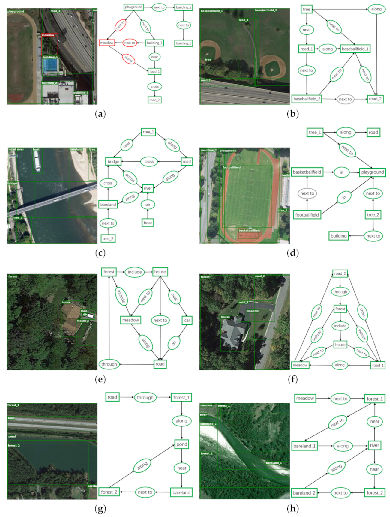
- RSSGD contains abundant ground-truth annotations corresponding to the remote sensing images as displayed in Figure 12, such as , , and so on, which play an irreplaceable role in improving the comprehensive and in-depth understanding on remote sensing scenes.
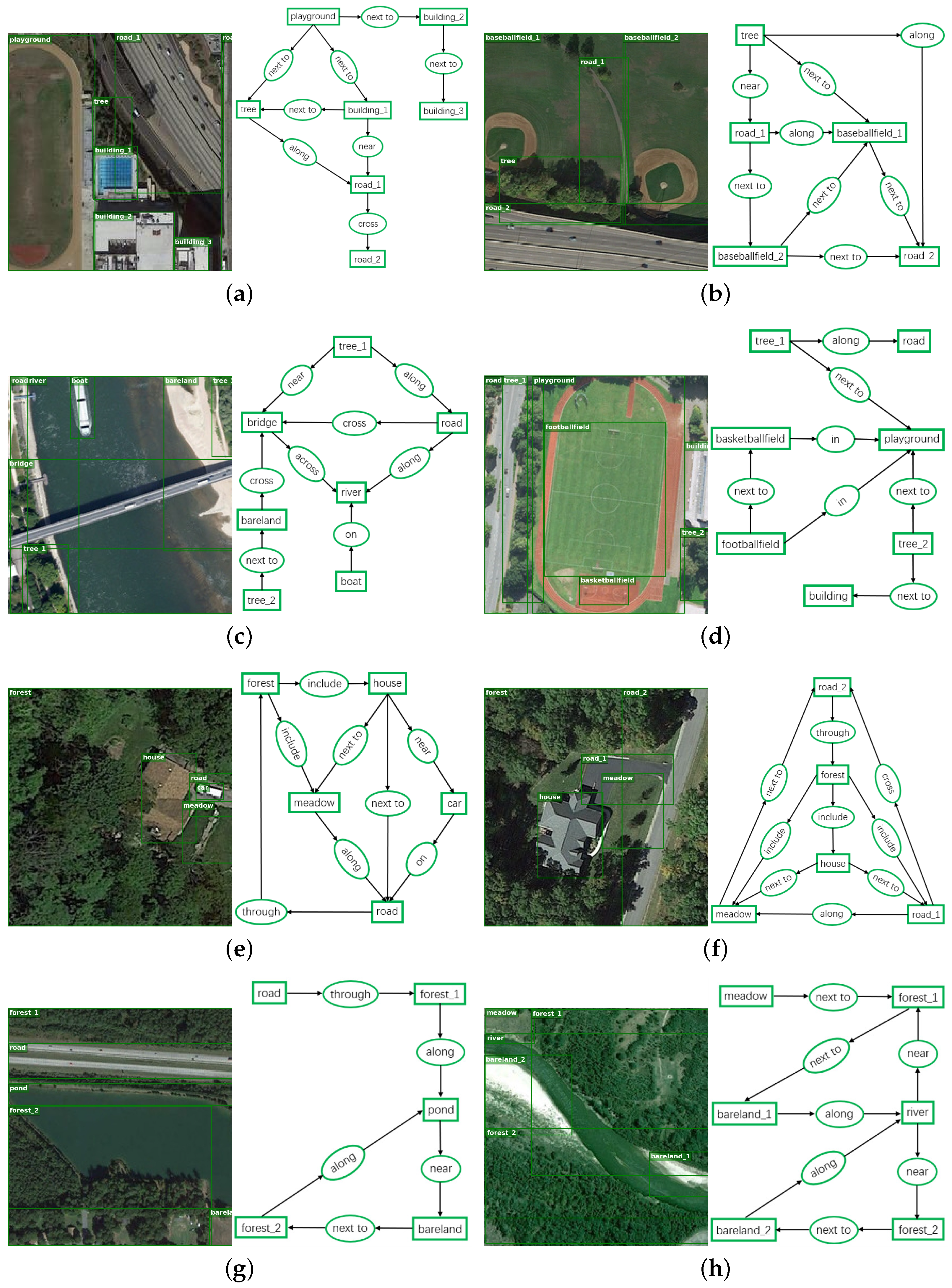
- From Figure 11 we can readily find that our model can accurately predict the relationships that are more appropriate for a particular scene. For example, in Figure 11e, the house is close to the meadow tightly, and our model precisely applies “next to” to represent the interactive relation among them. In contrast, the house is just near the car but not adjacent to it, so our model selects “near” to show the difference instead of still using “next to”. Likewise, in Figure 11c, the bridge and road are thin and long, so “cross” can correctly reflect the interaction between them. Furthermore, because the river is much wider than the road, so our method resourcefully employs “across” to emphasize the relationship between the bridge and the river from one side to the other. All the examples show a clear trend that our model is much more sensitive to those semantically informative relationships instead of the trivially biased ones.
- Similar to the previous works in scene graph parsing [39,42], Faster R-CNN [35] is used as the object detector in all experiments. However, this model cannot effectively extract deep visual features [66], which will inevitably interfere with the prediction on node categories. For instance, in Figure 11a, the tree is improperly identified as “meadow”, as a result, all of these detected relationships related to it are considered as negative.
5. Conclusions
In this paper, we propose a novel approach—MSFN—for remote sensing scene graph generation. In this framework, we adopt SREN, which is based on the mapping between visual features and semantic embeddings, to prevent invalid information from tainting valuable semantic context and improve the efficiency of scene graph construction. Besides, for effectively coping with the varied structure and size of ground objects, we introduce dilated convolution into graph convolutional network and propose MS-GCN to extend the cognitive horizon of our model. To further promote the research of remote sensing scene understanding, a novel relationship dataset—RSSGD—is proposed in this paper, which is used for establishing the connections from low-level feature perception to high-level semantic cognition. This dataset covers almost all common entities and relationships in remote sensing field. Furthermore, in order to avoid unbalanced bias of the model’s performance, there is no significant quantity difference between relation categories. Massive experiments are carried out on VG [49] dataset and RSSGD, and the results demonstrate that our approach achieves overwhelming advantages in predicting the semantic relations of remote sensing.
In addition, from Figure 9a we can find that the relationships contained in RSSGD are relatively simple. In order to further improve model’s cognitive ability to remote sensing scene, we will combine the property information of entities (e.g., size, shape, colour) and introduce multi-modal fusion technology in the future to mine more valuable semantic content, which is crucial to strengthen the understanding about remote sensing images.
Author Contributions
Conceptualization, Peng Li and Dezheng Zhang; methodology, Peng Li and Aziguli Wulamu; software, Peng Li and Peng Chen; investigation, Xin Liu and Peng Chen; writing—original draft, Peng Li and Xin Liu; writing—review and editing, Peng Li and Peng Chen; supervision, Dezheng Zhang; project administration, Dezheng Zhang; funding acquisition, Dezheng Zhang, Aziguli Wulamu and Xin Liu. All authors have read and agreed to the published version of the manuscript.
Funding
This research was supported in part by the National Key Research and Development Program of China under Grant 2018YFC0823002, in part by the Key Research and Development Program of Ningxia Hui Autonomous Region (Key Technologies for Intelligent Monitoring of Spatial Planning Based on High-Resolution Remote Sensing) under Grant 2019BFG02009, and in part by National Nature Science Foundation of China under Grant 61801019.
Institutional Review Board Statement
Not applicable.
Informed Consent Statement
Not applicable.
Data Availability Statement
The data presented in this study are available on request from the corresponding author. The data are not publicly available as they involve the subsequent application of patent, software copyright and the publication of project deliverables, and they are planned to be published at: https://github.com/lpsunny/RSSGD (accessed on 10 June 2021).
Conflicts of Interest
The authors declare no conflict of interest.
References
- Du, Z.; Li, X.; Lu, X. Local structure learning in high resolution remote sensing image retrieval. Neurocomputing 2016, 207, 813–822. [Google Scholar] [CrossRef]
- Gu, Y.; Wang, Q.; Xie, B. Multiple Kernel Sparse Representation for Airborne LiDAR Data Classification. IEEE Trans. Geosci. Remote Sens. 2017, 55, 1085–1105. [Google Scholar] [CrossRef]
- Lu, X.; Zheng, X.; Yuan, Y. Remote Sensing Scene Classification by Unsupervised Representation Learning. IEEE Trans. Geosci. Remote Sens. 2017, 55, 5148–5157. [Google Scholar] [CrossRef]
- Cheng, G.; Han, J.; Lu, X. Remote Sensing Image Scene Classification: Benchmark and State of the Art. Proc. IEEE 2017, 105, 1865–1883. [Google Scholar] [CrossRef] [Green Version]
- Maggiori, E.; Tarabalka, Y.; Charpiat, G.; Alliez, P. Convolutional Neural Networks for Large-Scale Remote-Sensing Image Classification. IEEE Trans. Geosci. Remote Sens. 2017, 55, 645–657. [Google Scholar] [CrossRef] [Green Version]
- Han, X.; Zhong, Y.; Zhang, L. An Efficient and Robust Integrated Geospatial Object Detection Framework for High Spatial Resolution Remote Sensing Imagery. Remote Sens. 2017, 9, 666. [Google Scholar] [CrossRef] [Green Version]
- Han, J.; Zhang, D.; Cheng, G.; Guo, L.; Ren, J. Object Detection in Optical Remote Sensing Images Based on Weakly Supervised Learning and High-Level Feature Learning. IEEE Trans. Geosci. Remote Sens. 2015, 53, 3325–3337. [Google Scholar] [CrossRef] [Green Version]
- Yuan, J.; Wang, D.; Li, R. Remote Sensing Image Segmentation by Combining Spectral and Texture Features. IEEE Trans. Geosci. Remote Sens. 2014, 52, 16–24. [Google Scholar] [CrossRef]
- Ma, F.; Gao, F.; Sun, J.; Zhou, H.; Hussain, A. Weakly Supervised Segmentation of SAR Imagery Using Superpixel and Hierarchically Adversarial CRF. Remote Sens. 2019, 11, 512. [Google Scholar] [CrossRef] [Green Version]
- Chen, F.; Ren, R.; de Voorde, T.V.; Xu, W.; Zhou, G.; Zhou, Y. Fast Automatic Airport Detection in Remote Sensing Images Using Convolutional Neural Networks. Remote Sens. 2018, 10, 443. [Google Scholar] [CrossRef] [Green Version]
- Dai, B.; Zhang, Y.; Lin, D. Detecting Visual Relationships with Deep Relational Networks. In Proceedings of the IEEE Conference on Computer Vision and Pattern Recognition, Honolulu, HI, USA, 21–26 July 2017; pp. 3298–3308. [Google Scholar] [CrossRef] [Green Version]
- Farhadi, A.; Hejrati, S.M.M.; Sadeghi, M.A.; Young, P.; Rashtchian, C.; Hockenmaier, J.; Forsyth, D.A. Every Picture Tells a Story: Generating Sentences from Images. In Proceedings of the 11th European Conference on Computer Vision, Heraklion, Greece, 5–11 September 2010; pp. 15–29. [Google Scholar] [CrossRef] [Green Version]
- Plummer, B.A.; Wang, L.; Cervantes, C.M.; Caicedo, J.C.; Hockenmaier, J.; Lazebnik, S. Flickr30k Entities: Collecting Region-to-Phrase Correspondences for Richer Image-to-Sentence Models. Int. J. Comput. Vis. 2017, 123, 74–93. [Google Scholar] [CrossRef] [Green Version]
- Torresani, L.; Szummer, M.; Fitzgibbon, A.W. Efficient Object Category Recognition Using Classemes. In Proceedings of the 11th European Conference on Computer Vision, Heraklion, Greece, 5–11 September 2010; pp. 776–789. [Google Scholar] [CrossRef]
- Lu, C.; Krishna, R.; Bernstein, M.S.; Li, F.F. Visual Relationship Detection with Language Priors. In Proceedings of the 14th European Conference on Computer Vision, Amsterdam, The Netherlands, 11–14 October 2016; pp. 852–869. [Google Scholar] [CrossRef] [Green Version]
- Karpathy, A.; Li, F.F. Deep Visual-Semantic Alignments for Generating Image Descriptions. IEEE Trans. Pattern Anal. Mach. Intell. 2017, 39, 664–676. [Google Scholar] [CrossRef] [Green Version]
- Xu, K.; Ba, J.; Kiros, R.; Cho, K.; Courville, A.C.; Salakhutdinov, R.; Zemel, R.S.; Bengio, Y. Show, Attend and Tell: Neural Image Caption Generation with Visual Attention. In Proceedings of the 32nd International Conference on Machine Learning, Lille, France, 6–11 July 2015; pp. 2048–2057. [Google Scholar]
- Ben-younes, H.; Cadène, R.; Thome, N.; Cord, M. BLOCK: Bilinear Superdiagonal Fusion for Visual Question Answering and Visual Relationship Detection. In Proceedings of the AAAI Conference on Artificial Intelligence, Honolulu, HI, USA, 27 January–1 February 2019; pp. 8102–8109. [Google Scholar] [CrossRef] [Green Version]
- Johnson, J.; Krishna, R.; Stark, M.; Li, L.; Shamma, D.A.; Bernstein, M.S.; Li, F.F. Image retrieval using scene graphs. In Proceedings of the IEEE Conference on Computer Vision and Pattern Recognition, Boston, MA, USA, 7–12 June 2015; pp. 3668–3678. [Google Scholar] [CrossRef]
- Li, Y.; Ouyang, W.; Zhou, B.; Shi, J.; Zhang, C.; Wang, X. Factorizable Net: An Efficient Subgraph-Based Framework for Scene Graph Generation. In Proceedings of the 15th European Conference on Computer Vision, Munich, Germany, 8–14 September 2018; pp. 346–363. [Google Scholar] [CrossRef] [Green Version]
- Qi, M.; Li, W.; Yang, Z.; Wang, Y.; Luo, J. Attentive Relational Networks for Mapping Images to Scene Graphs. In Proceedings of the IEEE Conference on Computer Vision and Pattern Recognition, Long Beach, CA, USA, 16–20 June 2019; pp. 3957–3966. [Google Scholar] [CrossRef] [Green Version]
- Klawonn, M.; Heim, E. Generating Triples With Adversarial Networks for Scene Graph Construction. In Proceedings of the AAAI Conference on Artificial Intelligence, New Orleans, LA, USA, 2–7 February 2018; pp. 6992–6999. [Google Scholar]
- Lu, X.; Wang, B.; Zheng, X.; Li, X. Exploring Models and Data for Remote Sensing Image Caption Generation. IEEE Trans. Geosci. Remote Sens. 2018, 56, 2183–2195. [Google Scholar] [CrossRef] [Green Version]
- Yu, F.; Koltun, V. Multi-Scale Context Aggregation by Dilated Convolutions. In Proceedings of the 4th International Conference on Learning Representations, San Juan, PR, USA, 2–4 May 2016. [Google Scholar]
- Qu, B.; Li, X.; Tao, D.; Lu, X. Deep semantic understanding of high resolution remote sensing image. In Proceedings of the International Conference on Computer Information and Telecommunication Systems, Kunming, China, 6–8 July 2016; pp. 1–5. [Google Scholar] [CrossRef]
- Shi, Z.; Zou, Z. Can a Machine Generate Humanlike Language Descriptions for a Remote Sensing Image? IEEE Trans. Geosci. Remote Sens. 2017, 55, 3623–3634. [Google Scholar] [CrossRef]
- Zhang, X.; Wang, X.; Tang, X.; Zhou, H.; Li, C. Description Generation for Remote Sensing Images Using Attribute Attention Mechanism. Remote Sens. 2019, 11, 612. [Google Scholar] [CrossRef] [Green Version]
- Wang, B.; Lu, X.; Zheng, X.; Li, X. Semantic Descriptions of High-Resolution Remote Sensing Images. IEEE Geosci. Remote Sens. Lett. 2019, 16, 1274–1278. [Google Scholar] [CrossRef]
- Bordes, A.; Usunier, N.; García-Durán, A.; Weston, J.; Yakhnenko, O. Translating Embeddings for Modeling Multi-relational Data. In Proceedings of the 27th Annual Conference on Neural Information Processing Systems, Lake Tahoe, NV, USA, 5–8 December 2013; pp. 2787–2795. [Google Scholar]
- Ladicky, L.; Russell, C.; Kohli, P.; Torr, P.H.S. Graph Cut Based Inference with Co-occurrence Statistics. In Proceedings of the 11th European Conference on Computer Vision, Heraklion, Greece, 5–11 September 2010; pp. 239–253. [Google Scholar] [CrossRef]
- Oliva, A.; Torralba, A. The role of context in object recognition. Trend. Cogn. Sci. 2007, 11, 520–527. [Google Scholar] [CrossRef]
- Parikh, D.; Zitnick, C.L.; Chen, T. From appearance to context-based recognition: Dense labeling in small images. In Proceedings of the IEEE Conference on Computer Vision and Pattern Recognition, Anchorage, AK, USA, 24–26 June 2008. [Google Scholar] [CrossRef]
- Rabinovich, A.; Vedaldi, A.; Galleguillos, C.; Wiewiora, E.; Belongie, S.J. Objects in Context. In Proceedings of the IEEE International Conference on Computer Vision, Rio de Janeiro, Brazil, 14–20 October 2007; pp. 1–8. [Google Scholar] [CrossRef]
- Girshick, R.B.; Donahue, J.; Darrell, T.; Malik, J. Rich Feature Hierarchies for Accurate Object Detection and Semantic Segmentation. In Proceedings of the IEEE Conference on Computer Vision and Pattern Recognition, Columbus, OH, USA, 23–28 June 2014; pp. 580–587. [Google Scholar] [CrossRef] [Green Version]
- Ren, S.; He, K.; Girshick, R.B.; Sun, J. Faster R-CNN: Towards Real-Time Object Detection with Region Proposal Networks. IEEE Trans. Pattern Anal. Mach. Intell. 2017, 39, 1137–1149. [Google Scholar] [CrossRef] [Green Version]
- Redmon, J.; Divvala, S.K.; Girshick, R.B.; Farhadi, A. You Only Look Once: Unified, Real-Time Object Detection. In Proceedings of the IEEE Conference on Computer Vision and Pattern Recognition, Las Vegas, NV, USA, 27–30 June 2016; pp. 779–788. [Google Scholar] [CrossRef] [Green Version]
- Schuster, S.; Krishna, R.; Chang, A.X.; Li, F.F.; Manning, C.D. Generating Semantically Precise Scene Graphs from Textual Descriptions for Improved Image Retrieval. In Proceedings of the Fourth Workshop on Vision and Language, Lisbon, Portugal, 18 September 2015; pp. 70–80. [Google Scholar] [CrossRef] [Green Version]
- Woo, S.; Kim, D.; Cho, D.; Kweon, I.S. LinkNet: Relational Embedding for Scene Graph. In Proceedings of the Annual Conference on Neural Information Processing Systems, Montréal, QC, Canada, 3–8 December 2018; pp. 558–568. [Google Scholar]
- Zhang, H.; Kyaw, Z.; Chang, S.; Chua, T. Visual Translation Embedding Network for Visual Relation Detection. In Proceedings of the IEEE Conference on Computer Vision and Pattern Recognition, Honolulu, HI, USA, 21–26 July 2017; pp. 3107–3115. [Google Scholar] [CrossRef] [Green Version]
- Xu, D.; Zhu, Y.; Choy, C.B.; Li, F.F. Scene Graph Generation by Iterative Message Passing. In Proceedings of the IEEE Conference on Computer Vision and Pattern Recognition, Honolulu, HI, USA, 21–27 July 2017; pp. 3097–3106. [Google Scholar] [CrossRef] [Green Version]
- Hu, R.; Rohrbach, M.; Andreas, J.; Darrell, T.; Saenko, K. Modeling Relationships in Referential Expressions with Compositional Modular Networks. In Proceedings of the IEEE Conference on Computer Vision and Pattern Recognition, Honolulu, HI, USA, 21–26 July 2017; pp. 4418–4427. [Google Scholar] [CrossRef] [Green Version]
- Zellers, R.; Yatskar, M.; Thomson, S.; Choi, Y. Neural Motifs: Scene Graph Parsing With Global Context. In Proceedings of the IEEE Conference on Computer Vision and Pattern Recognition, Salt Lake City, UT, USA, 18–22 June 2018; pp. 5831–5840. [Google Scholar] [CrossRef] [Green Version]
- Li, Y.; Ouyang, W.; Zhou, B.; Wang, K.; Wang, X. Scene Graph Generation from Objects, Phrases and Region Captions. In Proceedings of the IEEE International Conference on Computer Vision, Venice, Italy, 22–29 October 2017; pp. 1270–1279. [Google Scholar] [CrossRef] [Green Version]
- Hwang, S.J.; Ravi, S.N.; Tao, Z.; Kim, H.J.; Collins, M.D.; Singh, V. Tensorize, Factorize and Regularize: Robust Visual Relationship Learning. In Proceedings of the IEEE Conference on Computer Vision and Pattern Recognition, Salt Lake City, UT, USA, 18–22 June 2018; pp. 1014–1023. [Google Scholar] [CrossRef]
- Herzig, R.; Raboh, M.; Chechik, G.; Berant, J.; Globerson, A. Mapping Images to Scene Graphs with Permutation-Invariant Structured Prediction. In Proceedings of the Annual Conference on Neural Information Processing Systems, Montréal, QC, Canada, 3–8 December 2018; pp. 7211–7221. [Google Scholar]
- Yu, R.; Li, A.; Morariu, V.I.; Davis, L.S. Visual Relationship Detection with Internal and External Linguistic Knowledge Distillation. In Proceedings of the IEEE International Conference on Computer Vision, Venice, Italy, 22–29 October 2017; pp. 1068–1076. [Google Scholar] [CrossRef] [Green Version]
- Cui, Z.; Xu, C.; Zheng, W.; Yang, J. Context-Dependent Diffusion Network for Visual Relationship Detection. In Proceedings of the 26th ACM international conference on Multimedia, Seoul, Korea, 22–26 October 2018; pp. 1475–1482. [Google Scholar] [CrossRef] [Green Version]
- Lin, T.; Maire, M.; Belongie, S.J.; Hays, J.; Perona, P.; Ramanan, D.; Dollár, P.; Zitnick, C.L. Microsoft COCO: Common Objects in Context. In Proceedings of the 13th European Conferenceon Computer Vision, Zurich, Switzerland, 6–12 September 2014; pp. 740–755. [Google Scholar] [CrossRef] [Green Version]
- Krishna, R.; Zhu, Y.; Groth, O.; Johnson, J.; Hata, K.; Kravitz, J.; Chen, S.; Kalantidis, Y.; Li, L.; Shamma, D.A.; et al. Visual Genome: Connecting Language and Vision Using Crowdsourced Dense Image Annotations. Int. J. Comput. Vis. 2017, 123, 32–73. [Google Scholar] [CrossRef] [Green Version]
- Liang, Y.; Bai, Y.; Zhang, W.; Qian, X.; Zhu, L.; Mei, T. VrR-VG: Refocusing Visually-Relevant Relationships. In Proceedings of the IEEE/CVF International Conference on Computer Vision, Seoul, Korea, 2 November–27 October 2019; pp. 10402–10411. [Google Scholar] [CrossRef] [Green Version]
- Peyre, J.; Laptev, I.; Schmid, C.; Sivic, J. Weakly-Supervised Learning of Visual Relations. In Proceedings of the IEEE International Conference on Computer Vision, Venice, Italy, 22–29 October 2017; pp. 5189–5198. [Google Scholar] [CrossRef] [Green Version]
- Haut, J.M.; Fernández-Beltran, R.; Paoletti, M.E.; Plaza, J.; Plaza, A. Remote Sensing Image Superresolution Using Deep Residual Channel Attention. IEEE Trans. Geosci. Remote Sens. 2019, 57, 9277–9289. [Google Scholar] [CrossRef]
- Luo, H.; Chen, C.; Fang, L.; Zhu, X.; Lu, L. High-Resolution Aerial Images Semantic Segmentation Using Deep Fully Convolutional Network With Channel Attention Mechanism. IEEE J. Sel. Top. Appl. Earth Obs. Remote Sens. 2019, 12, 3492–3507. [Google Scholar] [CrossRef]
- Wang, J.; Shen, L.; Qiao, W.; Dai, Y.; Li, Z. Deep Feature Fusion with Integration of Residual Connection and Attention Model for Classification of VHR Remote Sensing Images. Remote Sens. 2019, 11, 1617. [Google Scholar] [CrossRef] [Green Version]
- Ba, R.; Chen, C.; Yuan, J.; Song, W.; Lo, S. SmokeNet: Satellite Smoke Scene Detection Using Convolutional Neural Network with Spatial and Channel-Wise Attention. Remote Sens. 2019, 11, 1702. [Google Scholar] [CrossRef] [Green Version]
- Li, J.; Xiu, J.; Yang, Z.; Liu, C. Dual Path Attention Net for Remote Sensing Semantic Image Segmentation. ISPRS Int. J. Geo-Inf. 2020, 9, 571. [Google Scholar] [CrossRef]
- Ren, S.; Zhou, F. Semi-Supervised Classification of PolSAR Data with Multi-Scale Weighted Graph Convolutional Network. In Proceedings of the IEEE International Geoscience and Remote Sensing Symposium, Waikoloa, HI, USA, 26 September–2 October 2020; pp. 1715–1718. [Google Scholar] [CrossRef]
- Wan, S.; Gong, C.; Zhong, P.; Du, B.; Zhang, L.; Yang, J. Multiscale Dynamic Graph Convolutional Network for Hyperspectral Image Classification. IEEE Trans. Geosci. Remote Sens. 2020, 58, 3162–3177. [Google Scholar] [CrossRef] [Green Version]
- Zhao, L.; Song, Y.; Zhang, C.; Liu, Y.; Wang, P.; Lin, T.; Deng, M.; Li, H. T-GCN: A Temporal Graph Convolutional Network for Traffic Prediction. IEEE Trans. Intell. Transp. Syst. 2020, 21, 3848–3858. [Google Scholar] [CrossRef] [Green Version]
- Shahraki, F.F.; Prasad, S. Graph Convolutional Neural Networks for Hyperspectral Data Classification. In Proceedings of the IEEE Global Conference on Signal and Information Processing, Anaheim, CA, USA, 26–29 November 2018; pp. 968–972. [Google Scholar] [CrossRef]
- Qin, A.; Shang, Z.; Tian, J.; Wang, Y.; Zhang, T.; Tang, Y.Y. Spectral-Spatial Graph Convolutional Networks for Semisupervised Hyperspectral Image Classification. IEEE Geosci. Remote Sens. Lett. 2019, 16, 241–245. [Google Scholar] [CrossRef]
- Wan, S.; Gong, C.; Zhong, P.; Pan, S.; Li, G.; Yang, J. Hyperspectral Image Classification With Context-Aware Dynamic Graph Convolutional Network. IEEE Trans. Geosci. Remote Sens. 2021, 59, 597–612. [Google Scholar] [CrossRef]
- Mou, L.; Lu, X.; Li, X.; Zhu, X.X. Nonlocal Graph Convolutional Networks for Hyperspectral Image Classification. IEEE Trans. Geosci. Remote Sens. 2020, 58, 8246–8257. [Google Scholar] [CrossRef]
- Khan, N.; Chaudhuri, U.; Banerjee, B.; Chaudhuri, S. Graph convolutional network for multi-label VHR remote sensing scene recognition. Neurocomputing 2019, 357, 36–46. [Google Scholar] [CrossRef]
- Shi, Y.; Li, Q.; Zhu, X.X. Building segmentation through a gated graph convolutional neural network with deep structured feature embedding. ISPRS J. Photogramm. Remote Sens. 2020, 159, 184–197. [Google Scholar] [CrossRef]
- Yang, J.; Lu, J.; Lee, S.; Batra, D.; Parikh, D. Graph R-CNN for Scene Graph Generation. In Proceedings of the 15th European Conference on Computer Vision, Munich, Germany, 8–14 September 2018; pp. 690–706. [Google Scholar] [CrossRef] [Green Version]
- Qiu, H.; Li, H.; Wu, Q.; Meng, F.; Ngan, K.N.; Shi, H. A2RMNet: Adaptively Aspect Ratio Multi-Scale Network for Object Detection in Remote Sensing Images. Remote Sens. 2019, 11, 1594. [Google Scholar] [CrossRef] [Green Version]
- Van der Maaten, L.; Hinton, G. Visualizing data using t-SNE. J. Mach. Learn. Res. 2008, 9, 2579–2605. [Google Scholar]
- Zhang, J.; Lin, S.; Ding, L.; Bruzzone, L. Multi-Scale Context Aggregation for Semantic Segmentation of Remote Sensing Images. Remote Sens. 2020, 12, 701. [Google Scholar] [CrossRef] [Green Version]
- Chen, L.; Papandreou, G.; Kokkinos, I.; Murphy, K.; Yuille, A.L. DeepLab: Semantic Image Segmentation with Deep Convolutional Nets, Atrous Convolution, and Fully Connected CRFs. IEEE Trans. Pattern Anal. Mach. Intell. 2018, 40, 834–848. [Google Scholar] [CrossRef]
- Li, G.; Müller, M.; Thabet, A.K.; Ghanem, B. DeepGCNs: Can GCNs Go As Deep As CNNs? In Proceedings of the IEEE/CVF International Conference on Computer Vision, Seoul, Korea, 27 October–2 November 2019; pp. 9266–9275. [Google Scholar] [CrossRef] [Green Version]
- Jaderberg, M.; Simonyan, K.; Zisserman, A.; Kavukcuoglu, K. Spatial Transformer Networks. In Proceedings of the Annual Conference on Neural Information Processing Systems, Montreal, QC, Canada, 7–12 December 2015; pp. 2017–2025. [Google Scholar]
- Andrews, M.; Chia, Y.K.; Witteveen, S. Scene Graph Parsing by Attention Graph. arXiv 2019, arXiv:1909.06273. [Google Scholar]
- Yang, Z.; Qin, Z.; Yu, J.; Hu, Y. Scene graph reasoning with prior visual relationship for visual question answering. arXiv 2018, arXiv:1812.09681. [Google Scholar]
- Tang, K.; Zhang, H.; Wu, B.; Luo, W.; Liu, W. Learning to Compose Dynamic Tree Structures for Visual Contexts. In Proceedings of the IEEE Conference on Computer Vision and Pattern Recognition, Long Beach, CA, USA, 16–20 June 2019; pp. 6619–6628. [Google Scholar] [CrossRef] [Green Version]
- Zhang, J.; Elhoseiny, M.; Cohen, S.; Chang, W.; Elgammal, A.M. Relationship Proposal Networks. In Proceedings of the IEEE Conference on Computer Vision and Pattern Recognition, Honolulu, HI, USA, 21–26 July 2017; pp. 5226–5234. [Google Scholar] [CrossRef]
- Hochreiter, S.; Schmidhuber, J. Long Short-Term Memory. Neural Comput. 1997, 9, 1735–1780. [Google Scholar] [CrossRef]
- Chen, T.; Yu, W.; Chen, R.; Lin, L. Knowledge-Embedded Routing Network for Scene Graph Generation. In Proceedings of the IEEE Conference on Computer Vision and Pattern Recognition, Long Beach, CA, USA, 16–20 June 2019; pp. 6163–6171. [Google Scholar] [CrossRef] [Green Version]
Figure 1.
The comparative illustration of object detection and scene graph. (a) The object detection result of baseballfield, in which nodes are annotated with region boxes and the belonging categories. (b) The scene graph corresponding to baseballfield, where the solid ellipses represent nodes and the lines with arrows represent the interactive relationships among nodes. (c) The object detection result of desert. (d) The scene graph corresponding to desert.

Figure 2.
The overview of our proposed MSFN.

Figure 4.
Three remote sensing scenes and the corresponding t-SNE [68] visualization.
Figure 4.
Three remote sensing scenes and the corresponding t-SNE [68] visualization.

Figure 5.
Illustration of semantic transformation. Mapping visual features (e.g., , ) and label embeddings (e.g., , ) to a common semantic space via the learned transformation matrixes (e.g., , ).
Figure 5.
Illustration of semantic transformation. Mapping visual features (e.g., , ) and label embeddings (e.g., , ) to a common semantic space via the learned transformation matrixes (e.g., , ).

Figure 6.
The receptive fields of 3 × 3 convolution kernel corresponding to different dilated rates. (a) has a receptive field of 3 × 3 when dilated rate is 1. (b) has a receptive field of 7 × 7 when dilated rate is 2. (c) has a receptive field of 15 × 15 when dilated rate is 3.
Figure 6.
The receptive fields of 3 × 3 convolution kernel corresponding to different dilated rates. (a) has a receptive field of 3 × 3 when dilated rate is 1. (b) has a receptive field of 7 × 7 when dilated rate is 2. (c) has a receptive field of 15 × 15 when dilated rate is 3.

Figure 7.
An illustration of multi-scale interaction. Rectangles represent nodes and diamonds represent relationships.
Figure 7.
An illustration of multi-scale interaction. Rectangles represent nodes and diamonds represent relationships.

Figure 8.
Quantity distribution of the main categories on RSSGD.

Figure 9.
Statistical results of the mainly relationships and attributes on RSSGD. (a) is the statistical result about relations. (b) is the statistical result about attributes.
Figure 9.
Statistical results of the mainly relationships and attributes on RSSGD. (a) is the statistical result about relations. (b) is the statistical result about attributes.

Figure 10.
Visualization results on RSSGD. (a) is the visualization result of object detection. (b) is the visualization result of scene understanding.
Figure 10.
Visualization results on RSSGD. (a) is the visualization result of object detection. (b) is the visualization result of scene understanding.

Figure 11.
The qualitative examples based on RSSGD. From (a–h) are the experimental results of object detection (left) and scene graph generation (right). In object detection, green boxes are the predicted nodes that matching with ground-truth labels, and red boxes denote the incorrect predictions. In relation reasoning, green ellipse is true positive predicted by our model, grey ellipse is false negative, and red ellipse is false positive. In order to keep the visualization interpretable, we only show the relationship predictions for the pairs of nodes that have ground-truth annotations.

Figure 12.
The ground-truth visualization on RSSGD. From (a–h) are the annotations of object detection (left) and scene graph generation (right) corresponding to Figure 11, which not only covers artificial scenes such as baseballfield and residential area, but also includes natural scenes such as river and pond.


Table 1.
The architecture of backbone network.
| Input Size | Convolution Kernel | Output Size | Number of Parameters |
|---|---|---|---|
| 224 × 224 | 3 × 3, 64 | 224 × 224 | (3 × 3 × 3) × 64 = 1728 |
| 224 × 224 | 3 × 3, 64 | 224 × 224 | (3 × 3 × 64) × 64 = 36,864 |
| Max Pooling | |||
| 112 × 112 | 3 × 3, 128 | 112 × 112 | (3 × 3 × 64) × 128 = 73,728 |
| 112 × 112 | 3 × 3, 128 | 112 × 112 | (3 × 3 × 128) × 128 = 147,456 |
| Max Pooling | |||
| 56 × 56 | 3 × 3, 256 | 56 × 56 | (3 × 3 × 128) × 256 = 294,912 |
| 56 × 56 | 3 × 3, 256 | 56 × 56 | (3 × 3 × 256) × 256 = 589,824 |
| 56 × 56 | 3 × 3, 256 | 56 × 56 | (3 × 3 × 256) × 256 = 589,824 |
| Max Pooling | |||
| 28 × 28 | 3 × 3, 512 | 28 × 28 | (3 × 3 × 256) × 512 = 1,179,684 |
| 28 × 28 | 3 × 3, 512 | 28 × 28 | (3 × 3 × 512) × 512 = 2,359,296 |
| 28 × 28 | 3 × 3, 512 | 28 × 28 | (3 × 3 × 512) × 512 = 2,359,296 |
| Max Pooling | |||
| 14 × 14 | 3 × 3, 512 | 14 × 14 | (3 × 3 × 512) × 512 = 2,359,296 |
| 14 × 14 | 3 × 3, 512 | 14 × 14 | (3 × 3 × 512) × 512 = 2,359,296 |
| 14 × 14 | 3 × 3, 512 | 14 × 14 | (3 × 3 × 512) × 512 = 2,359,296 |
Table 2.
Experimental results on VG [49] dataset.
Table 2.
Experimental results on VG [49] dataset.
| Model | PredCls | SGCls | SGGen | |||||||||
|---|---|---|---|---|---|---|---|---|---|---|---|---|
| IMP [40] | - | 10.1% | 10.8% | - | 6.0% | 6.1% | - | 3.7% | 4.9% | |||
| VTransE [39] | 7.6% | 12.4% | 14.3% | 4.9% | 6.8% | 7.2% | 3.2% | 5.3% | 5.8% | |||
| Motifs [42] | 11.3% | 14.2% | 15.4% | 6.2% | 8.0% | 8.3% | 4.4% | 6.0% | 7.2% | |||
| Graph R-CNN [66] | 13.1% | 18.8% | 22.6% | 7.9% | 9.7% | 11.1% | 4.9% | 6.8% | 8.6% | |||
| Knowledge-embedded [78] | 15.4% | 20.7% | 24.2% | 9.2% | 11.3% | 12.0% | 6.2% | 8.1% | 9.8% | |||
| VCTree [75] | 18.3% | 25.2% | 28.3% | 12.3% | 13.1% | 14.2% | 6.6% | 9.3% | 11.1% | |||
| Ours | SREN | AGCN | MS-GCN | |||||||||
| × | ✓ | × | 12.2% | 17.5% | 22.4% | 6.5% | 7.6% | 10.3% | 3.8% | 5.2% | 7.4% | |
| ✓ | ✓ | × | 14.4% | 19.6% | 24.3% | 8.1% | 9.2% | 11.8% | 4.6% | 6.4% | 9.2% | |
| ✓ | × | ✓ | 17.8% | 24.0% | 29.1% | 11.9% | 13.6% | 15.4% | 6.3% | 10.2% | 12.3% | |
Table 3.
Experimental results on RSSGD.
| Model | PredCls | SGCls | SGGen | |||||||||
|---|---|---|---|---|---|---|---|---|---|---|---|---|
| IMP [40] | - | 12.1% | 13.3% | - | 7.4% | 8.2% | - | 5.6% | 6.5% | |||
| VTransE [39] | 10.2% | 16.8% | 18.6% | 8.3% | 13.2% | 16.1% | 5.8% | 6.9% | 8.3% | |||
| Motifs [42] | 13.1% | 19.3% | 21.6% | 10.1% | 15.7% | 19.1% | 6.3% | 7.6% | 9.8% | |||
| Graph R-CNN [66] | 18.3% | 23.2% | 28.1% | 15.8% | 20.9% | 23.4% | 13.6% | 18.1% | 22.6% | |||
| Knowledge-embedded [78] | 20.4% | 25.1% | 30.7% | 17.3% | 22.6% | 25.6% | 15.2% | 19.4% | 24.4% | |||
| VCTree [75] | 21.6% | 27.4% | 31.6% | 18.8% | 23.3% | 27.2% | 16.1% | 20.7% | 25.2% | |||
| Ours | SREN | AGCN | MS-GCN | |||||||||
| × | ✓ | × | 17.2% | 22.4% | 27.0% | 14.3% | 20.3% | 22.6% | 11.8% | 17.2% | 21.3% | |
| ✓ | ✓ | × | 19.4% | 24.6% | 29.3% | 16.2% | 22.1% | 24.9% | 14.6% | 19.4% | 23.1% | |
| ✓ | × | ✓ | 23.7% | 28.9% | 34.2% | 20.1% | 26.3% | 29.1% | 18.3% | 23.6% | 27.4% | |
Publisher’s Note: MDPI stays neutral with regard to jurisdictional claims in published maps and institutional affiliations. |
© 2021 by the authors. Licensee MDPI, Basel, Switzerland. This article is an open access article distributed under the terms and conditions of the Creative Commons Attribution (CC BY) license (https://creativecommons.org/licenses/by/4.0/).
Share and Cite
MDPI and ACS Style
Li, P.; Zhang, D.; Wulamu, A.; Liu, X.; Chen, P. Semantic Relation Model and Dataset for Remote Sensing Scene Understanding. ISPRS Int. J. Geo-Inf. 2021, 10, 488. https://0-doi-org.brum.beds.ac.uk/10.3390/ijgi10070488
AMA Style
Li P, Zhang D, Wulamu A, Liu X, Chen P. Semantic Relation Model and Dataset for Remote Sensing Scene Understanding. ISPRS International Journal of Geo-Information. 2021; 10(7):488. https://0-doi-org.brum.beds.ac.uk/10.3390/ijgi10070488
Chicago/Turabian StyleLi, Peng, Dezheng Zhang, Aziguli Wulamu, Xin Liu, and Peng Chen. 2021. "Semantic Relation Model and Dataset for Remote Sensing Scene Understanding" ISPRS International Journal of Geo-Information 10, no. 7: 488. https://0-doi-org.brum.beds.ac.uk/10.3390/ijgi10070488
Note that from the first issue of 2016, this journal uses article numbers instead of page numbers. See further details here.