
A Process-Oriented Approach to Identify Evolutions of Sea Surface Temperature Anomalies with a Time-Series of a Raster Dataset


Abstract
:1. Introduction
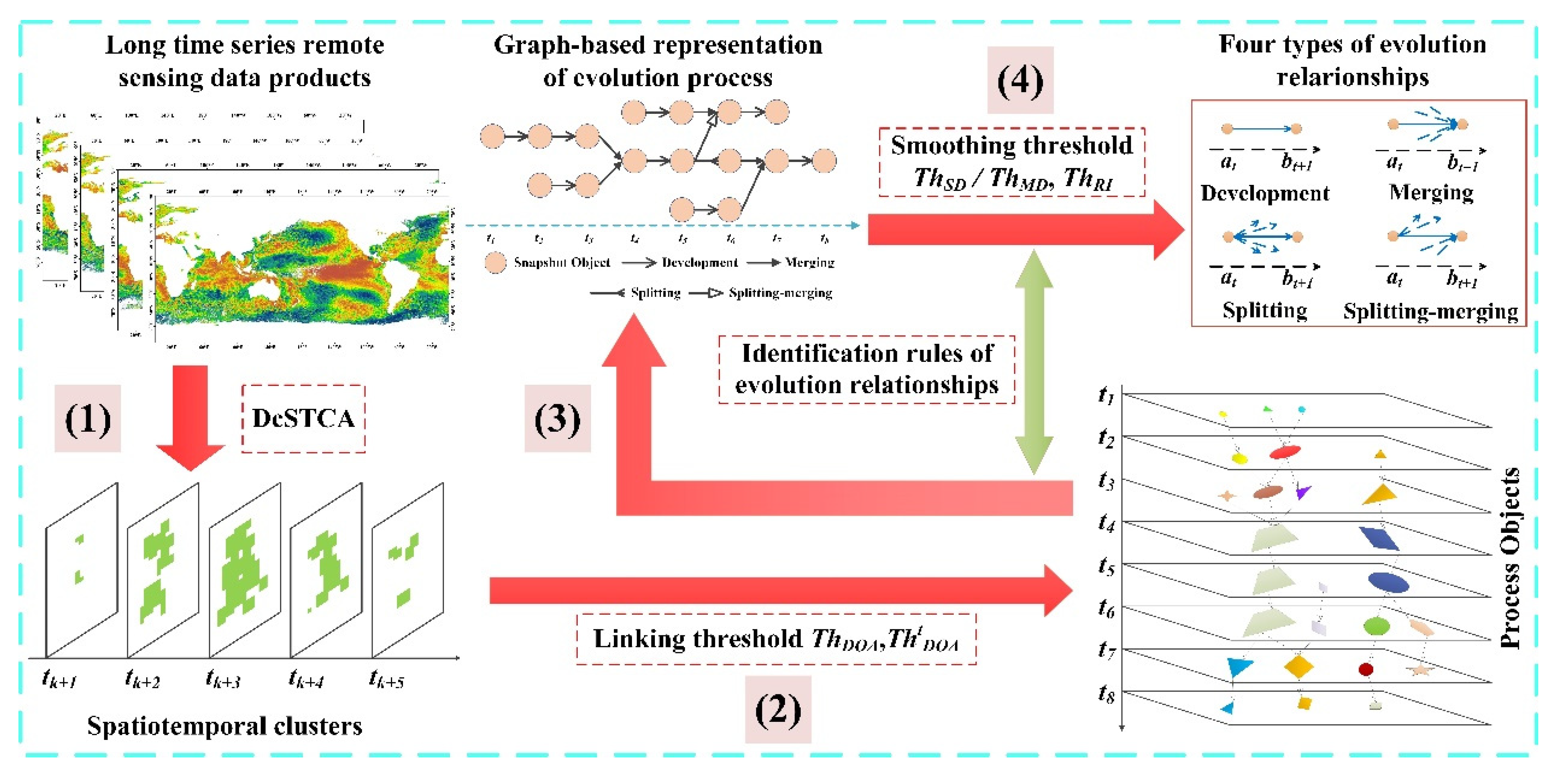
2. PoAIES Algorithm
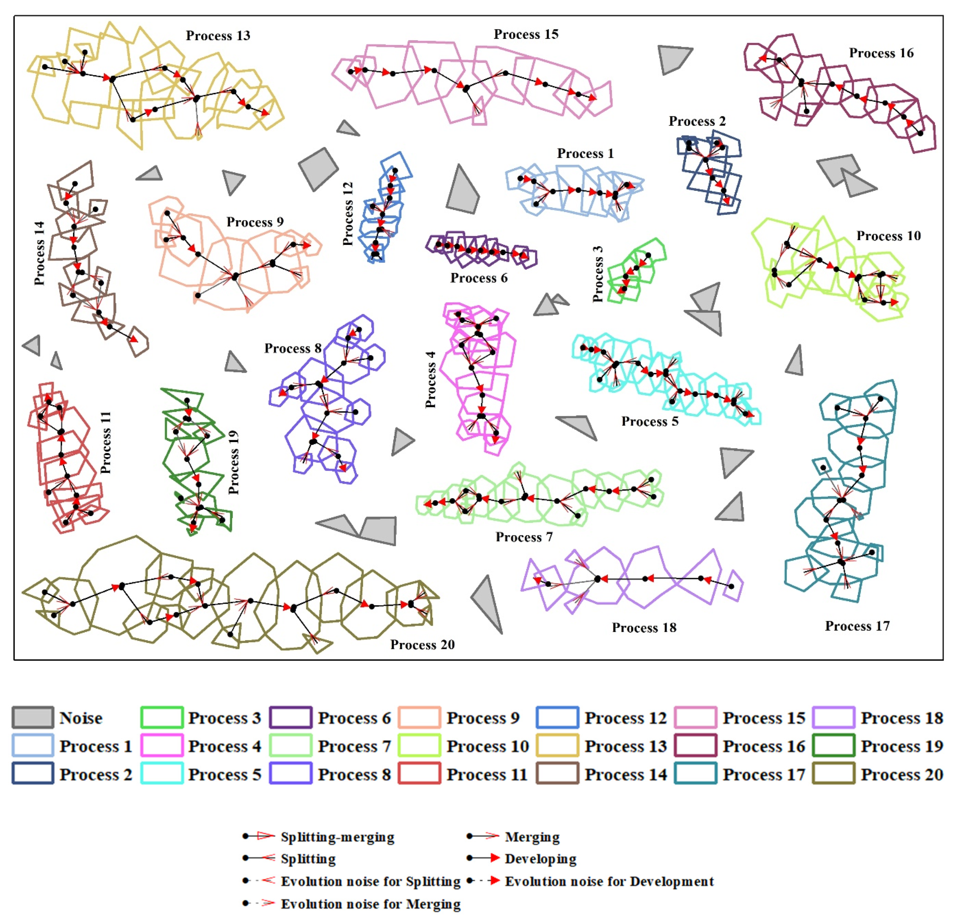
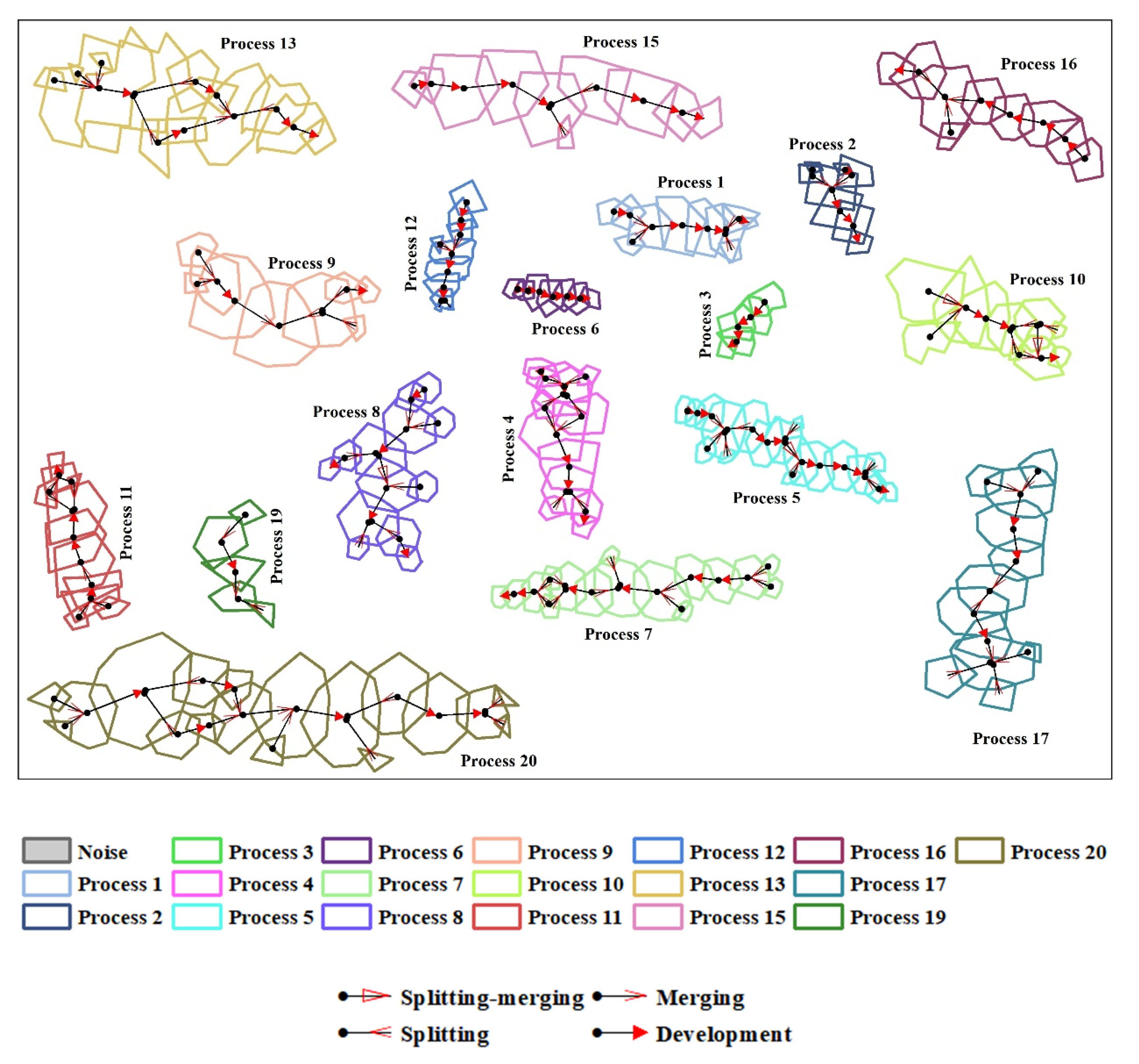
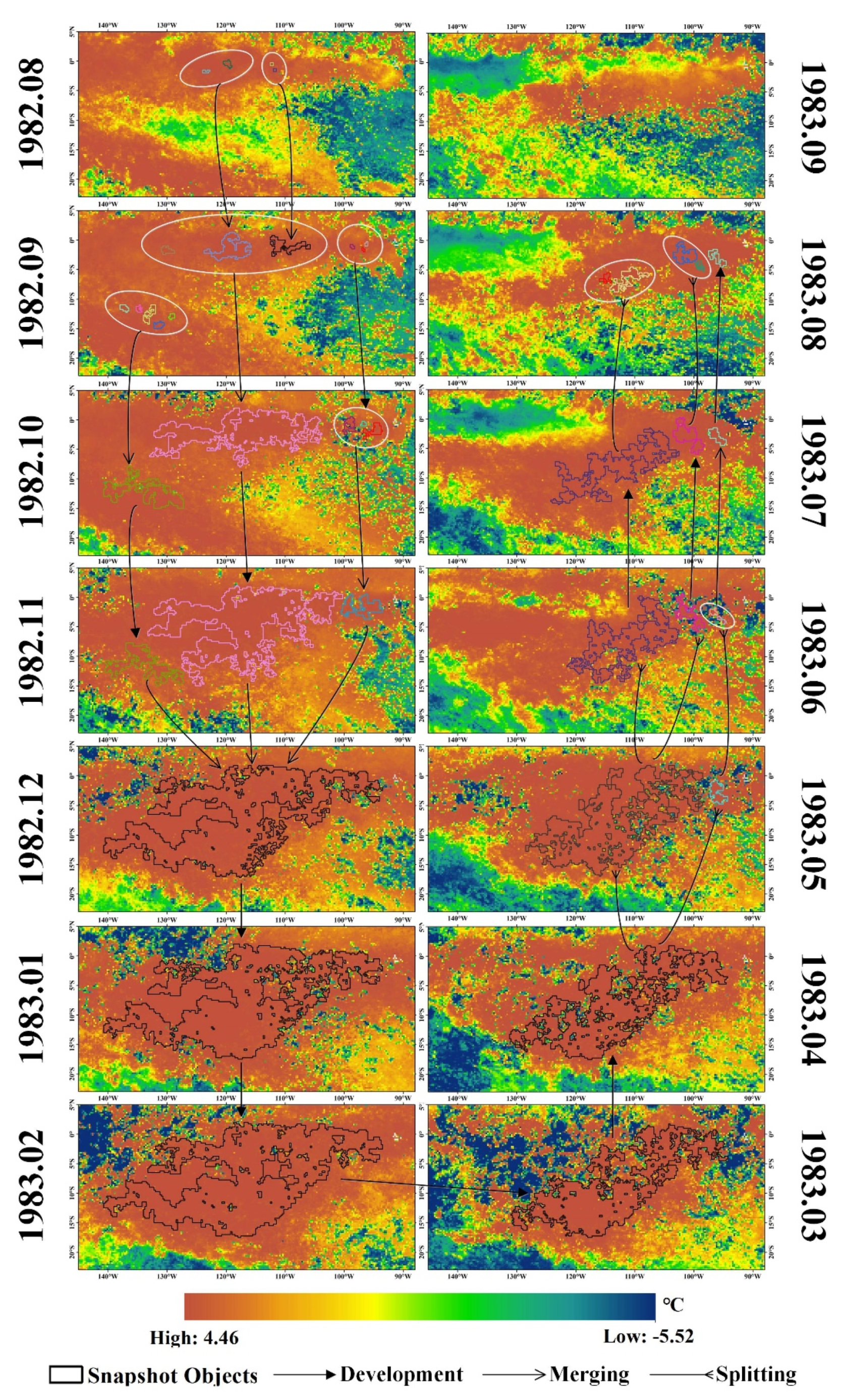
- A development relationship: Representing no interaction with other objects as one object moves from the previous to the current and then to the next snapshot.
- A merging relationship: Representing an interaction where two or more snapshot objects in the previous time snapshot merge into one object in the current time snapshot.
- A splitting relationship: Representing an interaction where one snapshot object in the current time snapshot split into two or more snapshot objects in the next time snapshot.
- A splitting/merging relationship: Representing an interaction where a part of one snapshot object and a part or whole of another snapshot object in the previous time snapshot merge into a new snapshot object in the current time snapshot.
2.1. Extracting Snapshot Objects of SSTA by an Enhanced DcSTCA
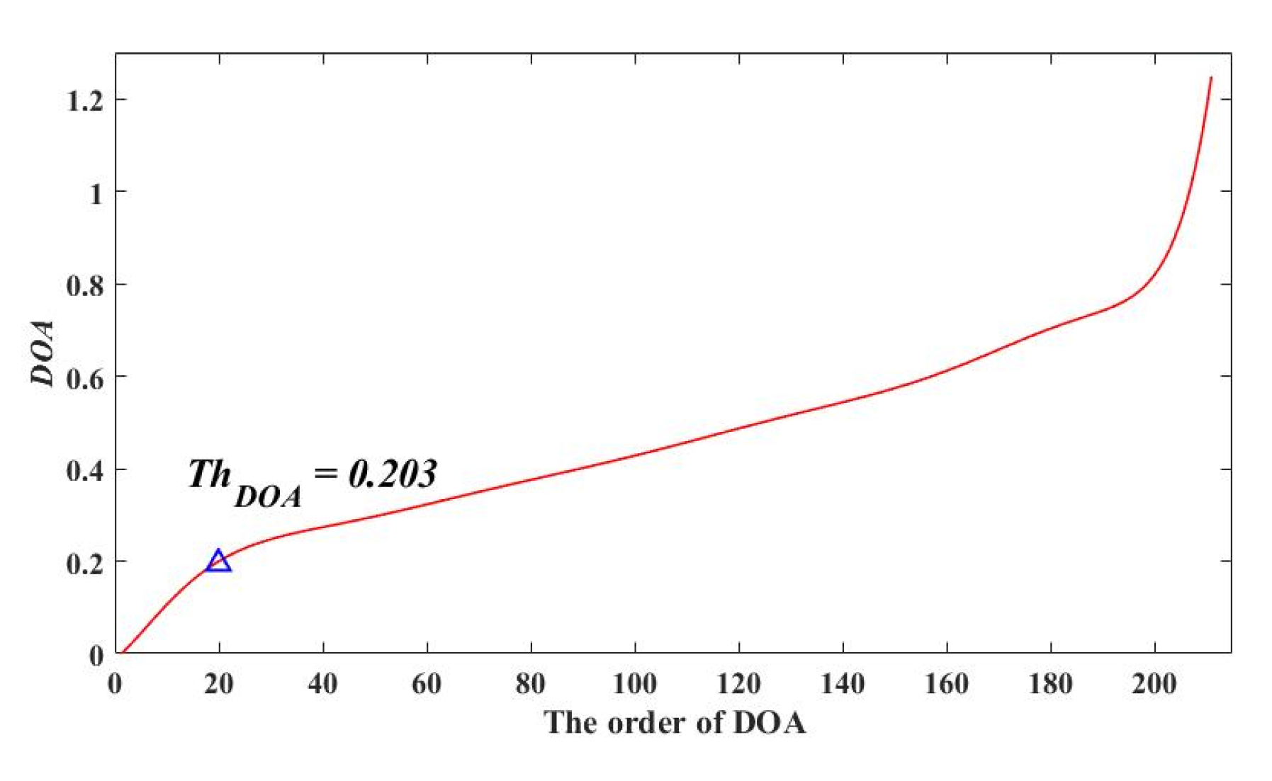
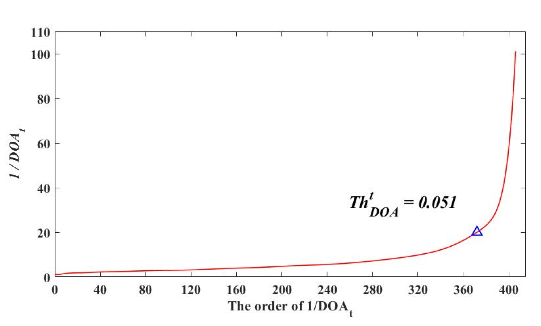
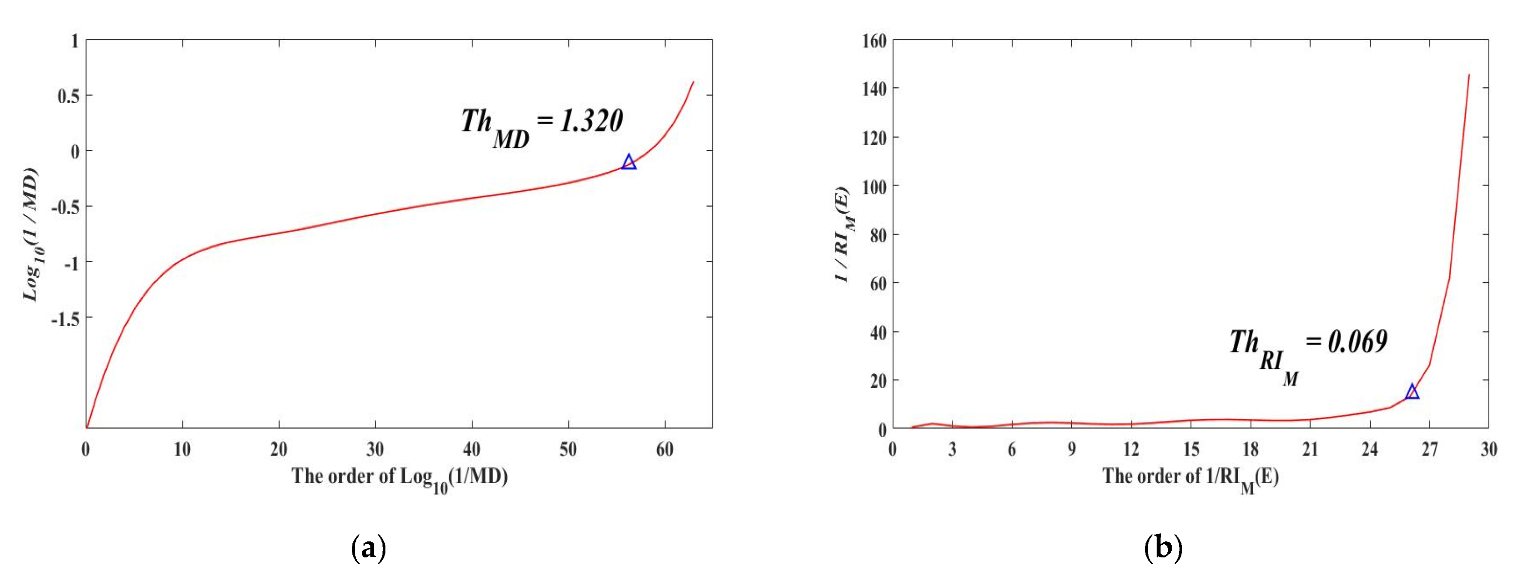
2.2. Determining an Optimal Linking Threshold to Construct Process Objects of SSTA
| Algorithm 1 |
| Step1: using Formula (1); Step2:s by an increasing order, and draw its curve; Step3:; Step4:. |
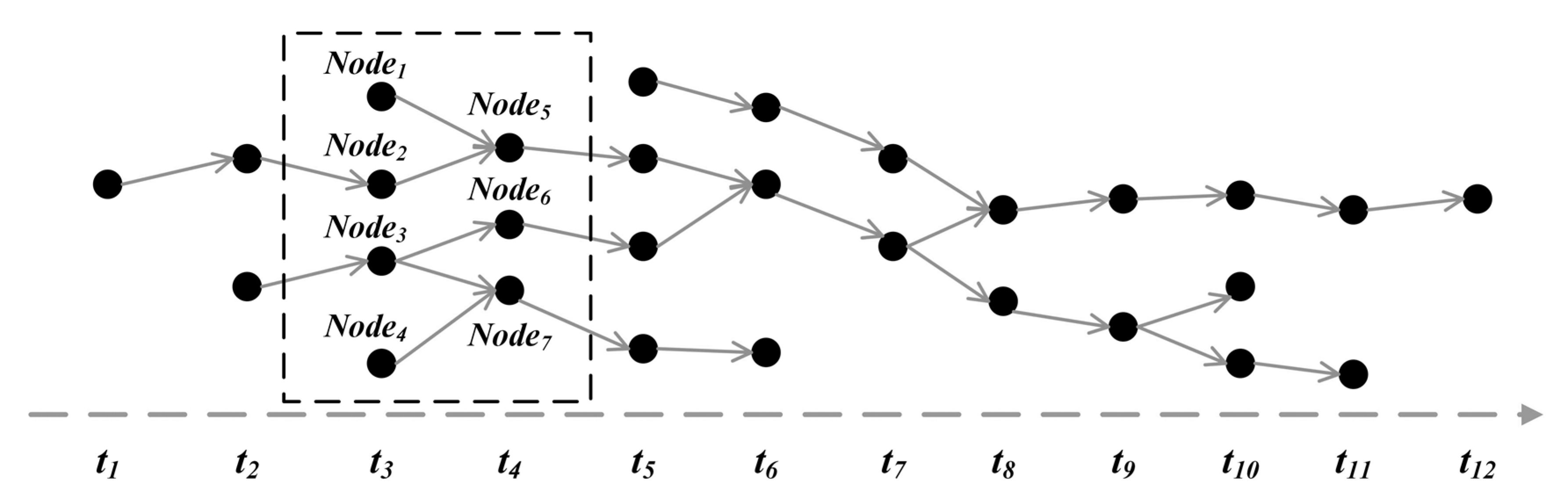
2.3. Graph-Based Representation on Process Objects
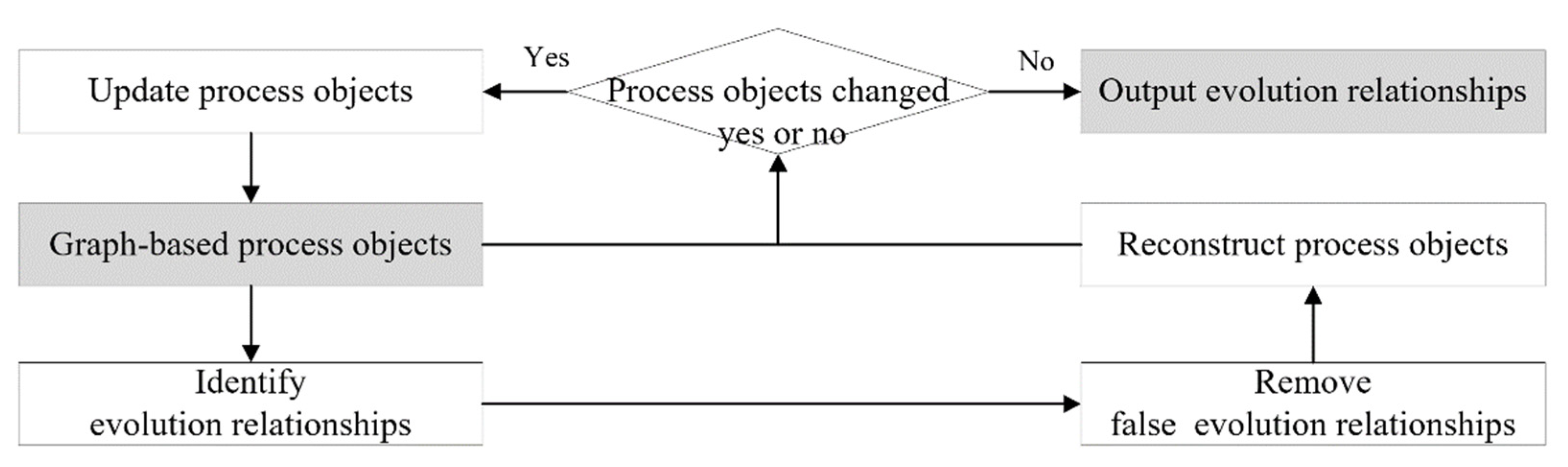
2.4. Identifying Evolution Relationships from Process Objects
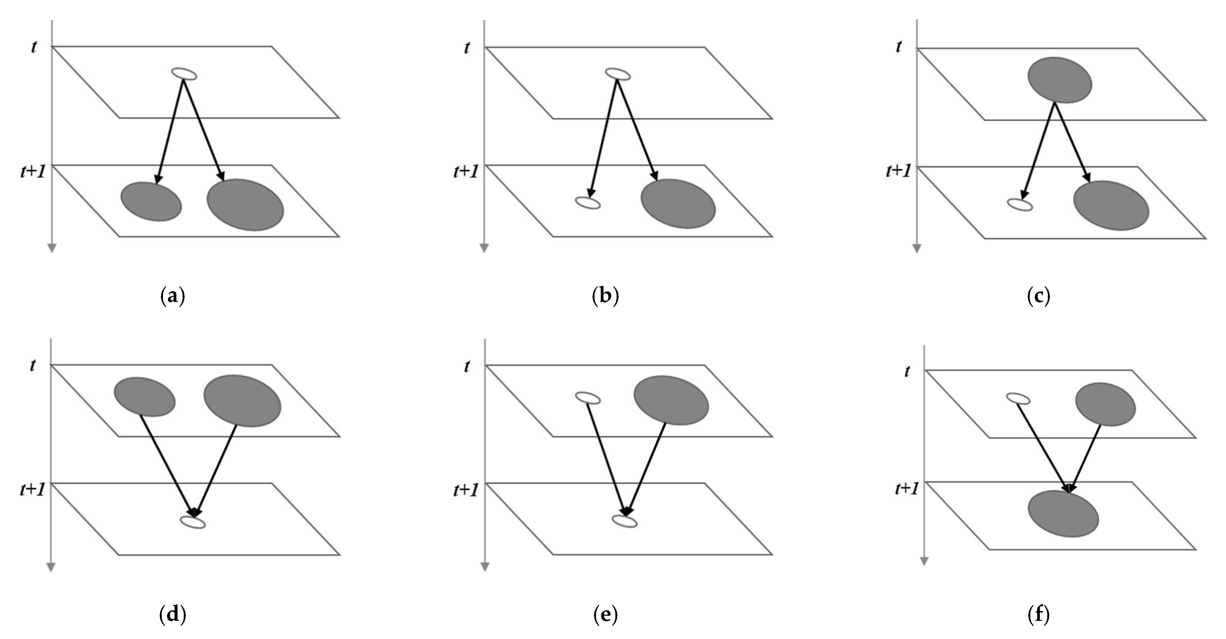
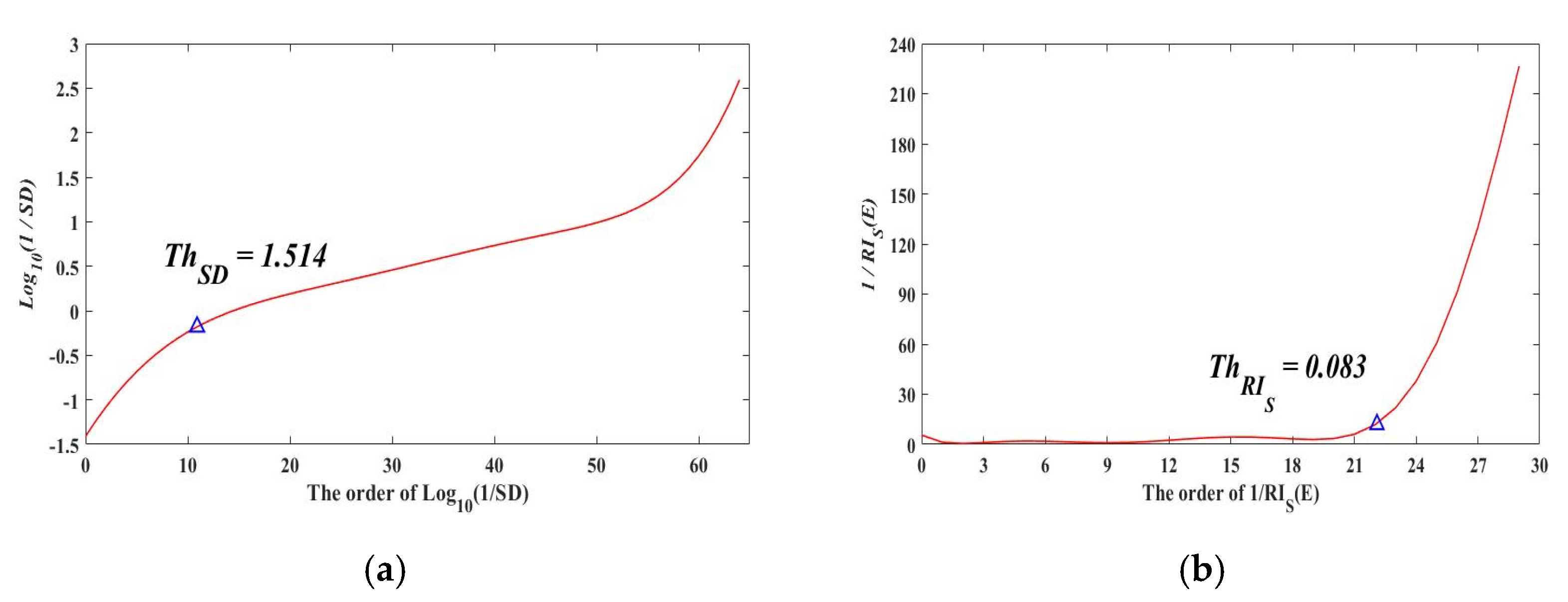
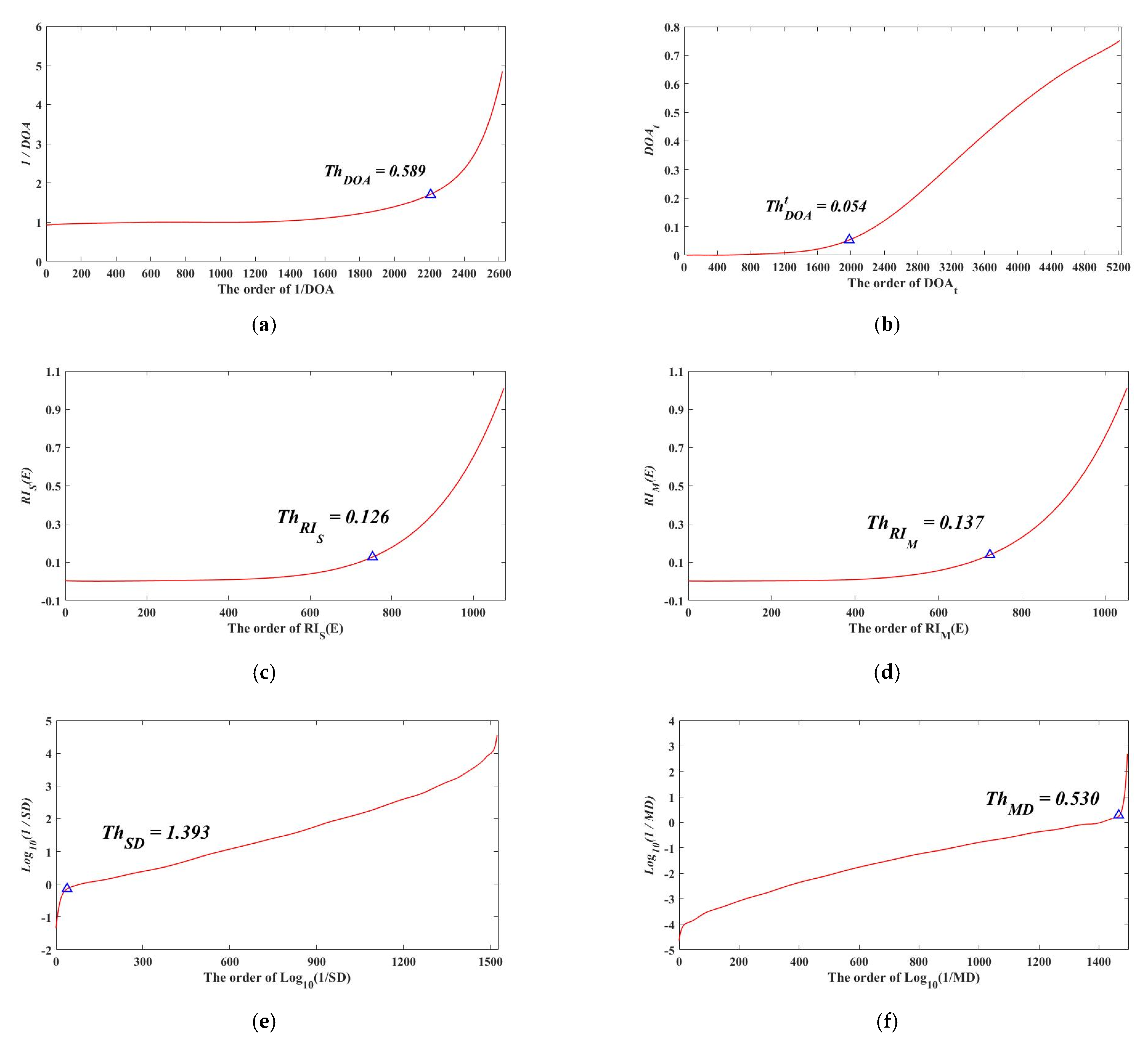
2.4.1. Remove False Evolution Relationships
| Algorithm 2 |
| Step1: using Formula (4)/ Formula (5)/ Formula (6)/ Formula (7); Step2: by an increasing order, and draw its curve; Step3:; Step4:. |
2.4.2. Identify True Evolution Relationships
3. Experiments and Evaluations
3.1. Simulated Dataset and Performance Analysis
3.1.1. Simulated Dataset
3.1.2. Thresholds and Performances
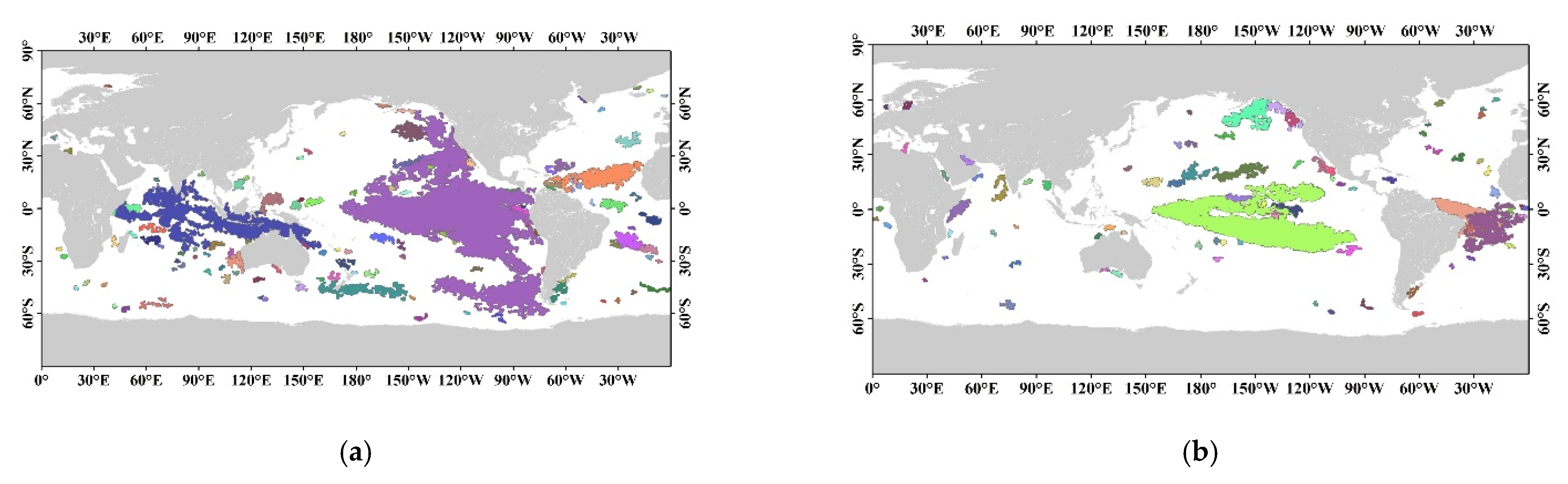
3.2. Dynamic Analysis of Process-Oriented SSTA Evolutions
3.2.1. A Remote-Sensing Dataset
3.2.2. Process-Oriented Objects of SSTA and their Evolutions
3.2.3. Relationships between SSTA Evolutions and ENSO
4. Conclusions
Author Contributions
Funding
Institutional Review Board Statement
Informed Consent Statement
Data Availability Statement
Acknowledgments
Conflicts of Interest
References
- Hollmann, R.; Merchant, C.; Saunders, R.; Downy, C.; Buchwitz, M.; Cazenave, A.; Chuvieco, E.; Defourny, P.; De Leeuw, G.; Forsberg, R.; et al. The ESA Climate Change Initiative: Satellite Data Records for Essential Climate Variables. Bull. Am. Meteorol. Soc. 2013, 94, 1541–1552. [Google Scholar] [CrossRef] [Green Version]
- Murtugudde, R.; Wang, L.; Hackert, E.; Beauchamp, J.; Christian, J.; Busalacchi, A.J. Remote sensing of the Indo-Pacific region: Ocean colour, sea level, winds and sea surface temperatures. Int. J. Remote Sens. 2004, 25, 1423–1435. [Google Scholar] [CrossRef]
- Dai, A. Future Warming Patterns Linked to Today’s Climate Variability. Sci. Rep. 2016, 6, 19110. [Google Scholar] [CrossRef] [Green Version]
- Xue, C.J.; Song, W.J.; Qin, L.J.; Dong, Q.; Wen, X. A spatiotemporal mining framework for abnormal association patterns in marine environments with a time series of remote sensing images. Int. J. Appl. Earth Obs. Geoinf. 2015, 38, 105–114. [Google Scholar] [CrossRef]
- McPhaden, M.J.; Zebiak, S.E.; Glantz, M.H. ENSO as an Integrating Concept in Earth Science. Science 2006, 314, 1740–1745. [Google Scholar] [CrossRef] [Green Version]
- Mcgregor, S.; Timmermann, A.; Schneider, N.; Stuecker, M.F.; England, M.H. The Effect of the South Pacific Convergence Zone on the Termination of El Niño Events and the Meridional Asymmetry of ENSO. J. Clim. 2012, 25, 5566–5586. [Google Scholar] [CrossRef] [Green Version]
- Ashok, K.; Behera, S.; Rao, S.A.; Weng, H.; Yamagat, H.W.A.T. El Niño Modoki and its possible teleconnection. J. Geophys. Res. Space Phys. 2007, 112, C11007. [Google Scholar] [CrossRef]
- Larkin, N.K.; Harrison, D.E. Global seasonal temperature and precipitation anomalies during El Niño autumn and winter. Geophys. Res. Lett. 2005, 32, L16705. [Google Scholar] [CrossRef]
- Yu, J.; Kao, H. Decadal changes of ENSO persistence barrier in SST and ocean heat content indices: 1958–2001. J. Geophys. Res. Atmos. 2007, 112, D13106. [Google Scholar] [CrossRef] [Green Version]
- Song, W.; Dong, Q.; Xue, C. A classified El Niño index using AVHRR remote-sensing SST data. Int. J. Remote Sens. 2016, 37, 403–417. [Google Scholar] [CrossRef]
- Ding, R.; Tseng, Y.; Li, J.; Sun, C.; Xie, F.; Hou, Z. Relative Contributions of North and South Pacific Sea Surface Temperature Anomalies to ENSO. J. Geophys. Res. Atmos. 2019, 124, 6222–6237. [Google Scholar] [CrossRef]
- Xue, C.; Wu, C.; Liu, J.; Su, F. A Novel Process-Oriented Graph Storage for Dynamic Geographic Phenomena. ISPRS Int. J. Geo-Inf. 2019, 8, 100. [Google Scholar] [CrossRef] [Green Version]
- Liu, J.Y.; Xue, C.J.; Dong, Q.; Wu, C.B.; Xu, Y.F. A Process-Oriented Spatiotemporal Clustering Method for Complex Trajectories of Dynamic Geographic Phenomena. IEEE Access 2019, 7, 155951–155964. [Google Scholar] [CrossRef]
- Yang, J.; Gong, P.; Fu, R.; Zhang, M.; Chen, J.; Liang, S.; Xu, B.; Shi, J.; Dickinson, R. Erratum: The role of satellite remote sensing in climate change studies. Nat. Clim. Chang. 2014, 3, 875–883. [Google Scholar] [CrossRef]
- Luo, W.; Yu, Z.-Y.; Xiao, S.-J.; Zhu, A.-X.; Yuan, L.-W. Exploratory Method for Spatio-Temporal Feature Extraction and Clustering: An Integrated Multi-Scale Framework. ISPRS Int. J. Geo-Inf. 2015, 4, 1870–1893. [Google Scholar] [CrossRef]
- Steinbach, M.; Tan, P.; Boriah, S.; Kumar, V.; Klooster, S.; Potter, C. The application of clustering to earth science data: Progress and challenges. In Proceedings of the 2nd NASA Data Mining Workshop: Issues and Applications in Earth Science Data, Pasadena, CA, USA, 23–24 May 2006; pp. 1–6. [Google Scholar]
- Birant, D.; Kut, A. ST-DBSCAN: An algorithm for clustering spatial–temporal data. Data Knowl. Eng. 2007, 60, 208–221. [Google Scholar] [CrossRef]
- Kawale, J.; Liess, S.; Kumar, A.; Steinbach, M.; Ganguly, A.; Samatova, N.F. Data guided discovery of dynamic climate dipoles. In Proceedings of the NASA Conference on Intelligent Data Understanding, Mountain View, CA, USA, 19–21 October 2011; pp. 30–44. [Google Scholar]
- Xue, C.; Dong, Q.; Qin, L. A cluster-based method for marine sensitive object extraction and representation. J. Ocean Univ. China 2015, 14, 612–620. [Google Scholar] [CrossRef]
- Liu, J.; Xue, C.; He, Y.; Dong, Q.; Kong, F.; Hong, Y. Dual-constraint Spatiotemporal Clustering Approach for Exploring Marine Anomaly Patterns using Remote Sensing Products. IEEE J. STARS 2018, 11, 3963–3976. [Google Scholar] [CrossRef]
- Long, J.A.; Weibel, R.; Dodge, S.; Laube, P. Moving ahead with computational movement analysis. Int. J. Geogr. Inf. Sci. 2018, 32, 1275–1281. [Google Scholar] [CrossRef] [Green Version]
- Dodge, S.; Gao, S.; Tomko, M.; Weibel, R. Progress in computational movement analysis—Towards movement data science. Int. J. Geogr. Inf. Sci. 2020, 34, 2395–2400. [Google Scholar] [CrossRef]
- Mondo, G.D.; Stell, J.G.; Claramunt, C.; Thibaud, R. A graph model for spatio-temporal evolution. J. Univers. Comput. Sci. 2010, 16, 1452–1477. [Google Scholar]
- Del Mondo, G.; Rodríguez, M.; Claramunt, C.; Bravo, L.; Thibaud, R. Modeling consistency of spatio-temporal graphs. Data Knowl. Eng. 2013, 84, 59–80. [Google Scholar] [CrossRef]
- Liu, W.; Li, X.; Rahn, D. Storm event representation and analysis based on a directed spatiotemporal graph model. Int. J. Geogr. Inf. Sci. 2016, 30, 1–22. [Google Scholar] [CrossRef]
- Zhu, R.; Guilbert, E.; Wong, M.S. Object-oriented tracking of the dynamic behavior of urban heat islands. Int. J. Geogr. Inf. Sci. 2017, 31, 405–424. [Google Scholar] [CrossRef] [Green Version]
- Dixon, M.; Wiener, G. TITAN: Thunderstorm identification, tracking, analysis, and nowcasting—A radar-based methodology. J. Atmos. Ocean. Technol. 1993, 10, 785–797. [Google Scholar] [CrossRef]
- Muñoz, C.; Wang, L.P.; Willems, P. Enhanced object-based tracking algorithm for convective rainstorms and cells. Atmos. Res. 2018, 201, 144–158. [Google Scholar] [CrossRef]
- Guttler, F.; Ienco, D.; Nin, J.; Teisseire, M.; Poncelet, P. A graph-based approach to detect spatiotemporal dynamics in satellite image time series. ISPRS J. Photogramm. Remote Sens. 2017, 130, 92–107. [Google Scholar] [CrossRef] [Green Version]
- Xue, C.; Dong, Q.; Xie, J. Marine spatio-temporal process semantics and its applications-taking the El Niño Southern Oscilation process and Chinese rainfall anomaly as an example. Acta Oceanol. Sin. 2012, 31, 16–24. [Google Scholar] [CrossRef]
- Xue, C.; Liu, J.; Yang, G.; Wu, C. A Process-Oriented Method for Tracking Rainstorms with a Time-Series of Raster Datasets. Appl. Sci. 2019, 9, 2468. [Google Scholar] [CrossRef] [Green Version]
- Shen, Z.Q.; Wan, R.C. A new approach for converting raster to vector—Node searching. J. Image and Graph. 1998, 3, 318–321. [Google Scholar]
- Robinson, I.; Webber, J.; Eifrem, E. Graph Database, 2nd ed.; O’Reilly Media, Inc.: Sebastopol, CA, USA, 2015. [Google Scholar]
- Zhang, P.S.; Steinbach, M.; Kumar, V.; Shekhar, S.; Tan, P. Discovery of patterns of Earth science data using data mining. In Next Generation of Data Mining Applications; Wiley: Piscataway, NJ, USA, 2005; pp. 167–188. [Google Scholar]
- Yan, H.; Sun, G.L.; Liu, X.D. Relationship between ENSO events and regional climate anomaliesaround the Xisha Islands during the last 50 years. J. Top. Oceanogr. 2010, 29, 29–35. [Google Scholar]
- Wiedermann, M.; Radebach, A.; Donges, J.F.; Kurths, J.; Donner, R.V. A climate network-based index to discriminate different types of El Niño and La Niña. Geophys. Res. Lett. 2016, 43, 7176–7185. [Google Scholar] [CrossRef] [Green Version]
- Zhang, Z.; Ren, B.; Zheng, J. A unified complex index to characterize two types of ENSO simultaneously. Sci. Rep. 2019, 9, 8373. [Google Scholar] [CrossRef]
- Kao, H.Y.; Yu, J.Y. Contrasting Eastern-Pacific and Central-Pacific Types of ENSO. J. Clim. 2009, 22, 615–632. [Google Scholar] [CrossRef]
- Kug, J.S.; Jin, F.F.; An, S.I. Two Types of El Niño Events: Cold Tongue El Niño and Warm Pool El Niño. J. Clim. 2009, 22, 1499–1515. [Google Scholar] [CrossRef]


| Evolution Relationship | Rule |
|---|---|
| Development (Objectt, Objectt+1) | The out degree of and the in degree of are both 1. |
| Splitting (Objectt, Objectt+1) | The out degree of is greater than 1 and the in degree of is 1. |
| Merging (Objectt, Objectt+1) | The out degree of is 1 and the in degree of is greater than 1. |
| Splitting/merging (Objectt, Objectt+1) | The out degree of and the in degree of are both greater than 1. |
| ProcessID | Stime | Etime | Nums | Number of Evolution Relationships | |||
|---|---|---|---|---|---|---|---|
| Development | Merging | Splitting | Splitting/Merging | ||||
| 1 | t1 | t8 | 10 | 5 | 2 | 2 | 0 |
| 2 | t3 | t8 | 8 | 5 | 2 | 0 | 0 |
| 3 | t2 | t6 | 5 | 4 | 0 | 0 | 0 |
| 4 | t5 | t14 | 13 | 5 | 4 | 4 | 0 |
| 5 | t1 | t13 | 18 | 8 | 3 | 5 | 1 |
| 6 | t7 | t15 | 9 | 8 | 0 | 0 | 0 |
| 7 | t4 | t15 | 16 | 6 | 6 | 4 | 0 |
| 8 | t7 | t14 | 13 | 5 | 3 | 3 | 1 |
| 9 | t10 | t16 | 11 | 2 | 4 | 4 | 0 |
| 10 | t13 | t20 | 12 | 3 | 2 | 6 | 2 |
| 11 | t9 | t17 | 12 | 4 | 6 | 2 | 0 |
| 12 | t12 | t19 | 11 | 4 | 2 | 4 | 0 |
| 13 | t10 | t18 | 14 | 5 | 5 | 4 | 0 |
| 14 | t12 | t20 | 11 | 5 | 4 | 2 | 0 |
| 15 | t11 | t19 | 10 | 7 | 0 | 2 | 0 |
| 16 | t13 | t20 | 10 | 5 | 2 | 2 | 0 |
| 17 | t10 | t18 | 14 | 3 | 6 | 4 | 0 |
| 18 | t15 | t20 | 8 | 4 | 0 | 3 | 0 |
| 19 | t9 | t16 | 12 | 4 | 4 | 4 | 0 |
| 20 | t8 | t19 | 18 | 6 | 6 | 6 | 0 |
| Accuracy | Precision | Recall | F1Score | |
|---|---|---|---|---|
| Snapshot object | 85.66 | 100.00 | 84.26 | 91.45 |
| Process object | 90.00 | 100.00 | 90.00 | 94.74 |
| Evolution relationship | 94.20 | 98.88 | 94.15 | 96.46 |
| Type | No. of Process Objects | No. of Snapshot Objects | Evolution Relationship | |
|---|---|---|---|---|
| Type | Num | |||
| Warm | 122 | 2701 | Development | 1510 |
| Splitting | 388 | |||
| Merging | 417 | |||
| Splitting/merging | 12 | |||
| Cold | 86 | 1335 | Development | 751 |
| Splitting | 215 | |||
| Merging | 220 | |||
| Splitting/merging | 10 | |||
| Type of SSTA | Development Stage of ENSO | Evolution Relationship of Process Object | |
|---|---|---|---|
| Merging | Splitting | ||
| Warm | Strengthening | 83.87% | 16.13% |
| Weakening | 24.58% | 75.42% | |
| Cold | Strengthening | 85.11% | 14.89% |
| Weakening | 27.35% | 72.65% | |
Publisher’s Note: MDPI stays neutral with regard to jurisdictional claims in published maps and institutional affiliations. |
© 2021 by the authors. Licensee MDPI, Basel, Switzerland. This article is an open access article distributed under the terms and conditions of the Creative Commons Attribution (CC BY) license (https://creativecommons.org/licenses/by/4.0/).
Share and Cite
Li, L.; Xu, Y.; Xue, C.; Fu, Y.; Zhang, Y. A Process-Oriented Approach to Identify Evolutions of Sea Surface Temperature Anomalies with a Time-Series of a Raster Dataset. ISPRS Int. J. Geo-Inf. 2021, 10, 500. https://0-doi-org.brum.beds.ac.uk/10.3390/ijgi10080500
Li L, Xu Y, Xue C, Fu Y, Zhang Y. A Process-Oriented Approach to Identify Evolutions of Sea Surface Temperature Anomalies with a Time-Series of a Raster Dataset. ISPRS International Journal of Geo-Information. 2021; 10(8):500. https://0-doi-org.brum.beds.ac.uk/10.3390/ijgi10080500
Chicago/Turabian StyleLi, Lianwei, Yangfeng Xu, Cunjin Xue, Yuxuan Fu, and Yuanyu Zhang. 2021. "A Process-Oriented Approach to Identify Evolutions of Sea Surface Temperature Anomalies with a Time-Series of a Raster Dataset" ISPRS International Journal of Geo-Information 10, no. 8: 500. https://0-doi-org.brum.beds.ac.uk/10.3390/ijgi10080500