RSPCN: Super-Resolution of Digital Elevation Model Based on Recursive Sub-Pixel Convolutional Neural Networks

Abstract

The digital elevation model (DEM) is known as one kind of the most significant fundamental geographical data models. The theory, method and application of DEM are hot research issues in geography, especially in geomorphology, hydrology, soil and other related fields. In this paper, we improve the efficient sub-pixel convolutional neural networks (ESPCN) and propose recursive sub-pixel convolutional neural networks (RSPCN) to generate higher-resolution DEMs (HRDEMs) from low-resolution DEMs (LRDEMs). Firstly, the structure of RSPCN is described in detail based on recursion theory. This paper explores the effects of different training datasets, with the self-adaptive learning rate Adam algorithm optimizing the model. Furthermore, the adding-“zero” boundary method is introduced into the RSPCN algorithm as a data preprocessing method, which improves the RSPCN method’s accuracy and convergence. Extensive experiments are conducted to train the method till optimality. Finally, comparisons are made with other traditional interpolation methods, such as bicubic, nearest-neighbor and bilinear methods. The results show that our method has obvious improvements in both accuracy and robustness and further illustrate the feasibility of deep learning methods in the DEM data processing area.

1. Introduction

The digital elevation model (DEM [1]) is a digital simulation of a terrain surface using limited terrain elevation data, which contains rich topographic information for the application and analysis of geosciences [2]. DEM has the characteristics of simple geographical data organization, intuitive terrain information representation and efficient terrain factor interpretation. It is widely used in geomorphology, hydrology, soil and other related fields and plays an important role in the practice of surveying and mapping, soil and water conservation, hydrogeological disaster monitoring and controlling and land use managing and planning [3]. Resolution in our paper denotes “pixel size”, which is an important index for DEM to describe the size of the smallest unit. It is important to explore terrain modeling solutions for generating higher-resolution DEMs (HRDEMs) from captured low-resolution DEMs (LRDEMs) [4,5,6], referred to as super resolution (SR) solutions. During the process of SR, a clearer image is reconstructed by using the information of at least one low-resolution image [7,8,9,10]. SR technology has high application need and application prospect, especially for applications that demand higher-resolution and higher-fidelity terrain information. There are some examples: (1) real-time terrain simulations serving for vehicle route planning and fast adaptation; (2) realistic terrain rendering technology used for ranging simulations, entertainment and 3D high realistic gaming graphic environments [5]; (3) the SR mode on satellites (such as SPOT5 satellite) to achieve HRDEMs from low-resolution cameras [11,12]. In our study, we focus on the terrain modeling process of LRDEMs with an aim to obtain HRDEMs terrain models with high fidelity to the real terrain structures.

The image SR algorithm was first proposed by Tsai and Huang [13]. Since then, many researchers have been dedicated to SR algorithms [14,15,16,17,18]. Currently, SR algorithms are usually classified into three types: interpolative types, reconstructive types and learning types [19]. The interpolation methods [14,20,21,22,23,24,25,26] are commonly used and have good results on terrain modeling, such as the bilinear algorithm [27,28], bicubic interpolation [29,30], inverse distance to a power [31,32], the radial basis function [10], the spline function [33], Coons surface [34,35], the numerical approximation expression [36,37,38], the statistical method of cross validation [39], the recursive algorithm [40], wavelet transformation [41], Delaunay triangulation interpolation [42], B-splines [43], etc. After the deep learning (DL) algorithm became popular, the SR algorithm based on DL appeared in 2014 [44]. Researchers have proposed a variety of classic DL-based super-Resolution algorithms, such as iterative back projection [45], maximum likelihood estimate [46], maximum a posterior [47,48], multi-task learning [49], support vector regression [50], super resolution convolutional neural networks (SRCNN) [44], etc. Then, researches began focusing not only on images but also on videos and higher dimensional multimedia data, especially DEMs [51,52].

The landmark work on DL-based SR is based on the convolutional neural networks (CNN) model for single image super-resolution (SISR), called SRCNN [44,53]. However, due to the simple three-layer convolution structure [54,55] of SRCNN, it usually causes over-smooth errors for severely changing terrain data [56] and a long computational time. Many improved SRCNN algorithms have been studied. For example, Dong et al. [57,58] and Shi et al. [59] presented modified SRCNN algorithms to speed up the feature extraction process by directly dealing with sub-feature maps or sub-pixel convolution layers. Deeply recursive cortical networks [60] were proposed to reduce the depth of CNN and improve the calculation efficiency and training stability. Lim et al. [61] proposed an optimized version of the ResNet structure for SR in their enhanced deep residual networks for SISR. O. Argudo et al. [6], Ashish A Kubade et al. [5] and Mengjiao Qin et al. [62] added information from aerial images or remote sensing images to increase the DEM resolution. However, there is still great potential for visualization based on SR [63].

In this paper, we introduce efficient sub-pixel convolutional neural networks (ESPCN) [59] into the DEM SR process and propose the recursive sub-pixel convolutional neural networks (RSPCN) to build HRDEMs. The proposed method is like an interpolator that over-samples the DEM, which starts with a single image and ends with the same single image but with a finer density of pixels. Compared with the SRCNN method, our RSPCN method recursively deals with sub-pixel convolution layers and speeds up the feature extraction process. Compared with other traditional interpolation methods (bicubic, bilinear, nearest-neighbor), it eases the over-smooth issues and improves the accuracy. Compared with ESPCN, it introduces recursive idea and reduces the depth of networks. The results imply that it is especially useful for visualization applications, such as real-time terrain simulations and realistic terrain rendering.

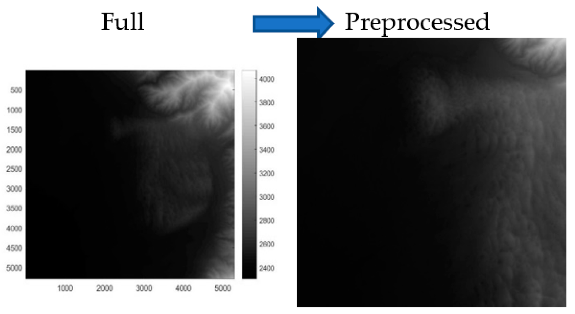
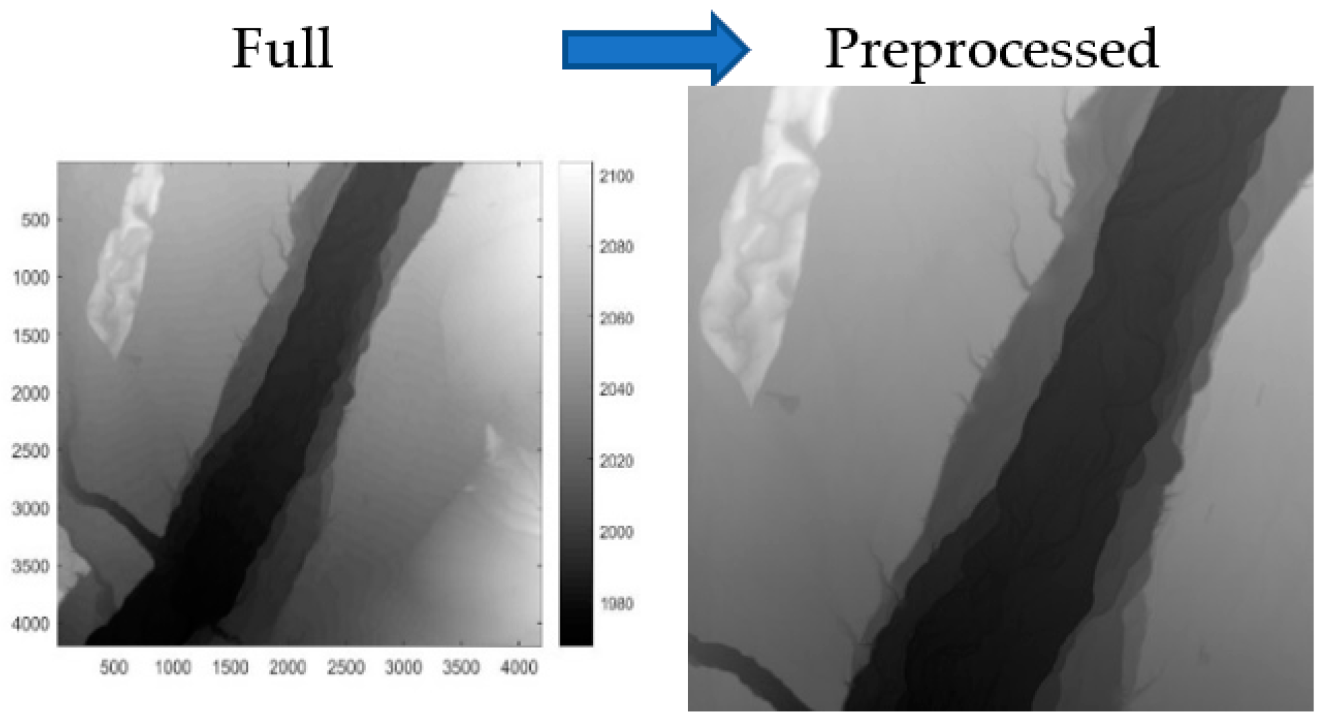
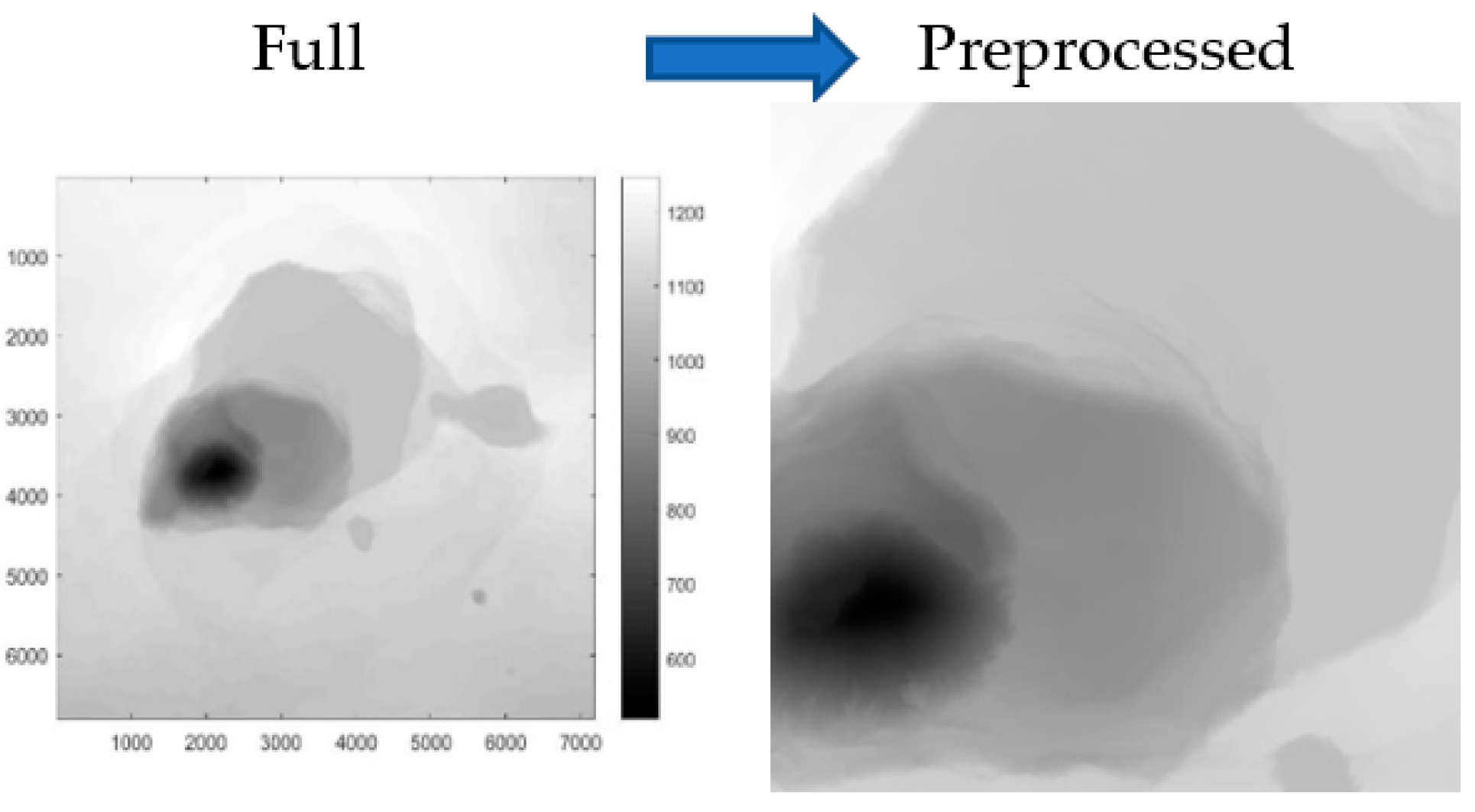
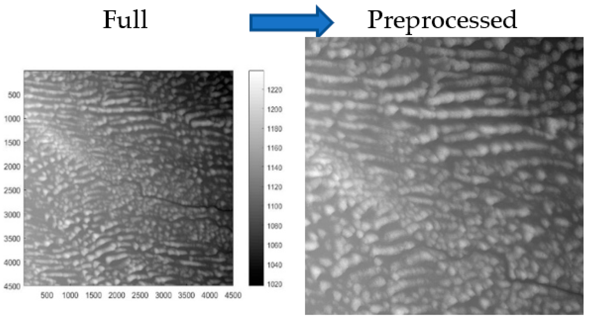
2. Study Datasets and Data Preprocess

To show and compare different terrain modeling methods in a straightforward manner, we chose a publicly available collection [64] of single-scale elevation models of representative landforms as our experimental datasets. These HRDEMs of archetypal landform types are derived from the United States Geological Survey (USGS) 3D Elevation Program (3DEP) LiDAR sources with resolution ranging from 2 to 10 m. The six archetypal landform datasets include an eroded plateau (Bryce Canyon, UT, USA, Figure 1, Full), a volcanic caldera (Crater Lake, OR, USA, Figure 2, Full), active sand dunes (Great Sand Dunes, CO, USA, Figure 3, Full), a braided riverbed (Jackson Hole, WY, USA, Figure 4, Full), a shield caldera (Kīlauea, HI, USA, Figure 5, Full) and stabilized sand dunes (Sandhills, NE, USA, Figure 6, Full). The datasets are intercepted and made into the same size DEM of 1000 $\times$ 1000 by downsampling DEMs with medium interval from above DEMs. Then, these six classes of datasets are normalized, as shown in Formula (1), shown as preprocessed DEMs in Figure 1, Figure 2, Figure 3, Figure 4, Figure 5 and Figure 6. Finally, we obtain 500$\times$500 LRDEMs by downsampling DEMs with medium interval from 1000$\times$1000 DEMs. These 500$\times$500 preprocessed datasets are obtained as experimental DEMs, the detailed information about which is shown in

Table 1. The detailed information of six study areas and experimental datasets (500 $\times$ 500).

	Details	Pixel Size (m)	Projection	Data Source	Data Processing
Experimental Datasets
Bryce Canyon		6	UTM/NAD83 Zone 12	3DEP	downsampled from 3 to 6 m
Crater Lake		19.8	UTM/NAD83 Zone 10N	3DEP	downsampled from 9.9 to 19.8 m
Great Sand Dunes		19.8	UTM/NAD83 Zone 13N	3DEP	downsampled from 9.9 to 19.8 m
Jackson Hole		12	UTM/NAD83 Zone 12N	3DEP	downsampled from 6 to 12 m
Kīlauea		6	UTM/NAD83 Zone 5	airborne Lidar U.S. Geological Survey	downsampled from 3 to 6 m
Sandhills		60	UTM/NAD83 Zone 14N	3DEP	downsampled from 30 to 60 m

.

$$\{\begin{array}{c}\mathit{x}\left(i,j\right)=\frac{\mathit{x}\left(i,j\right)-\min \left\{\mathit{x}\left(i,j\right)\right\}}{\max \left\{\mathit{x}\left(i,j\right)\right\}-\min \left\{\mathit{x}\left(i,j\right)\right\}}\\ \mathit{y}\left(i,j\right)=\frac{\mathit{y}\left(i,j\right)-\min \left\{\mathit{y}\left(i,j\right)\right\}}{\max \left\{\mathit{y}\left(i,j\right)\right\}-\min \left\{\mathit{y}\left(i,j\right)\right\}}\end{array}.$$

(1)

3. Methodology

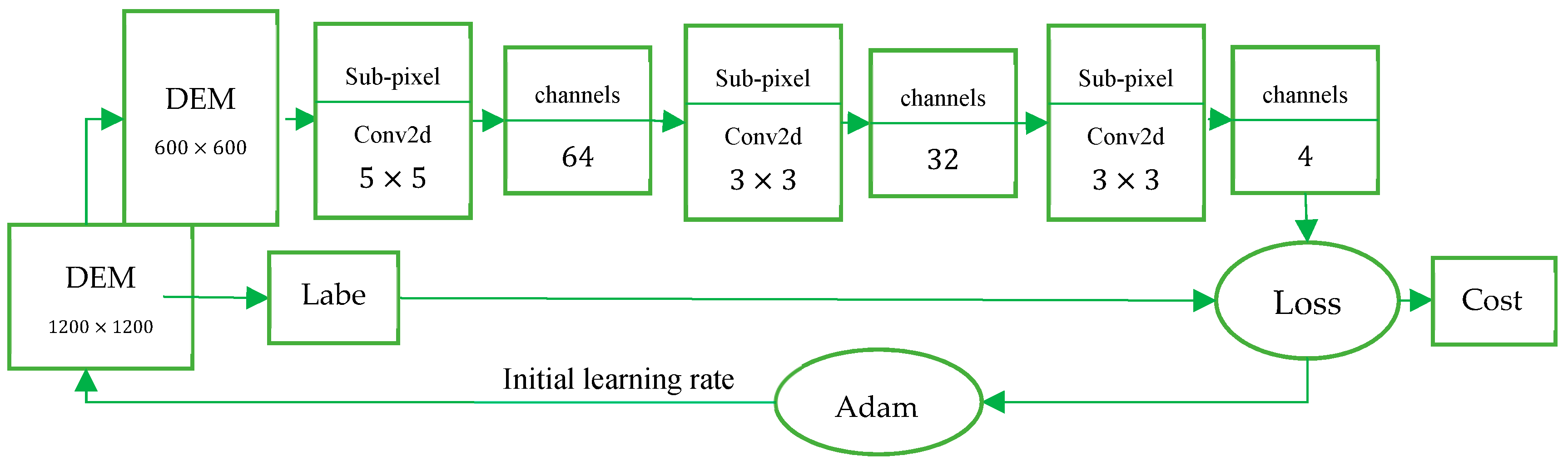
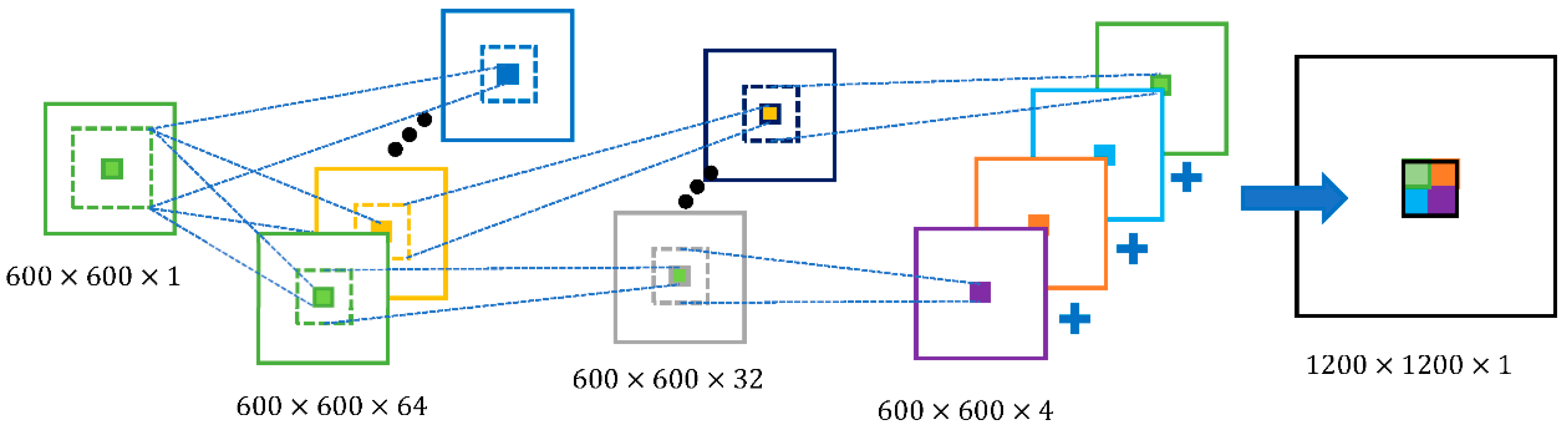
3.1. Efficient Sub-Pixel Convolutional Neural Networks (ESPCN)

The specific process of the algorithm is as follows: LRDEM data are used as the input data into the network, which enter into the three sub-pixel convolutional layers using rectified linear unit (ReLU) as activation function. After entering into the first sub-pixel convolutional layer with kernel 4 × 4, the datasets will turn into 64-channel datasets. Then, second sub-pixel convolutional layer with kernel 3 × 3 finally outputs 4-channel datasets, which means that the length and width of the DEM grid data increases by one time, respectively. The self-adaptive learning rate Adam [65] algorithm is used to optimize the model. The specific structure of our method is shown in Figure 7. The process of the data formation is shown in Figure 8.

In our method, we use common loss function in the network and mean-square error (MSE) between the real DEM data $x_{i,j}$ and the generated super-resolution DEM data $y_{i,j}$, as shown in Formula (2), where $n$ is the square matrix’s number of rows/columns.

$$Cost=\frac{{{\displaystyle \sum }}_{i=1}^n{{\displaystyle \sum }}_{j=1}^n{\left(x_{i,j}-y_{i,j}\right)}^2}{n^2}$$

(2)

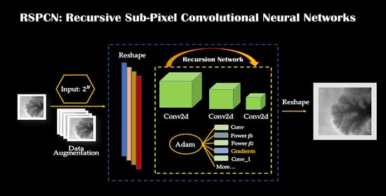
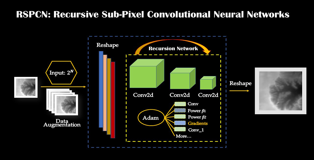
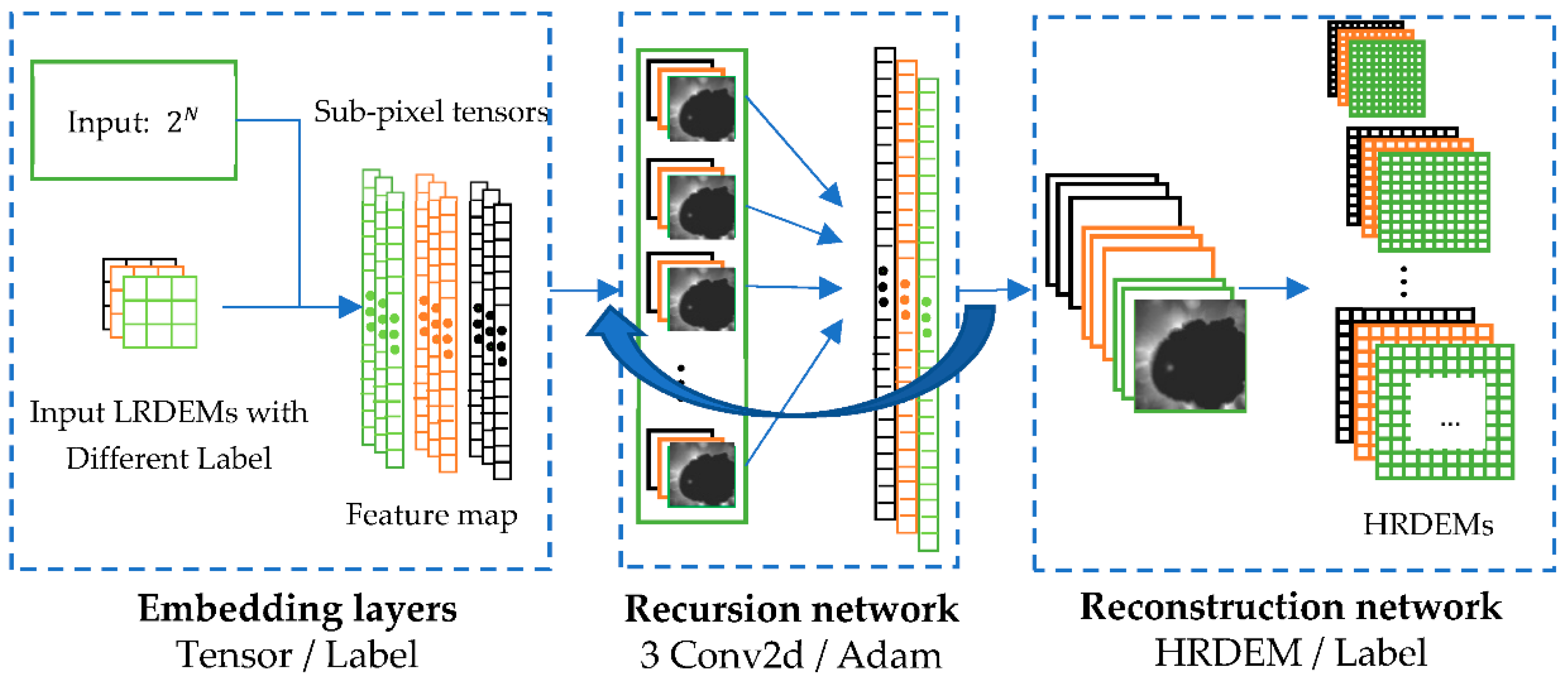
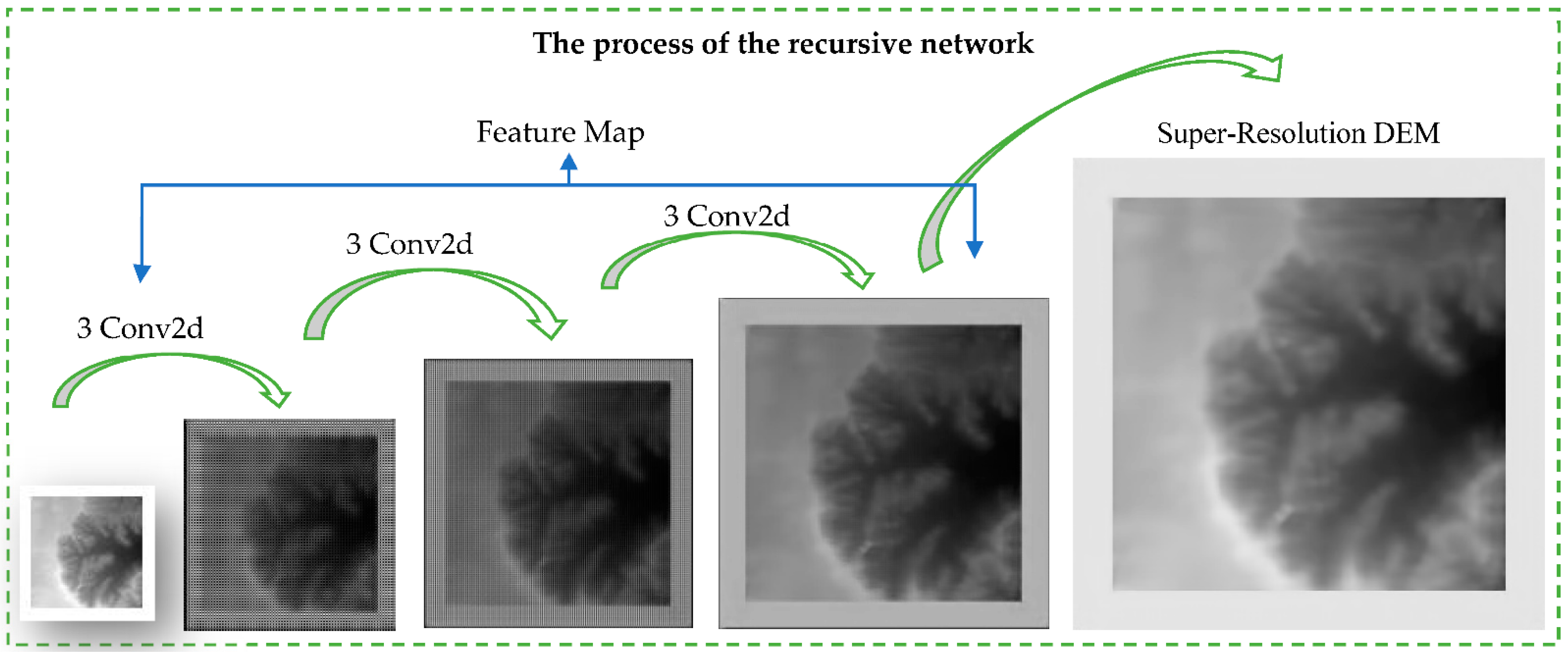
3.2. Recursive Sub-Pixel Convolutional Neural Networks (RSPCN)

Based on ESPCN, the proposed RSPCN model is presented by introducing the idea of recursion. The network is outlined in Figure 9, containing three sub-networks: embedding, recursion and reconstruction networks. The embedding network is used to generate feature maps from LRDEMs. Next, the recursion part finishes the SR part. After this, final feature maps in the recursion part are fed into the reconstruction network to generate the output HRDEMs.

The embedding network takes the input LRDEMs and extracts their features. The input parameter $N$ denotes magnification factor. Firstly, LRDEMs are normalized and turned into binary codes. Secondly, six different types of terrain are labeled as tensors (from 0 to 5). Finally, these tensors will be passed into the recursion layer.

The recursion network is the main network, containing recursive three-layer CNN to solve the task of SR. Every recursive step completes one ESPCN process with the parameter $n$ counting, until $n=N$. Meanwhile, every recursion makes the cell size of DEM smaller and outputs the tensors with labels.

The reconstruction network transforms these tensors (2 channel) back into the LRDEM space (3 channel), generating HRDEMs of different terrain.

4. Experiments and Results

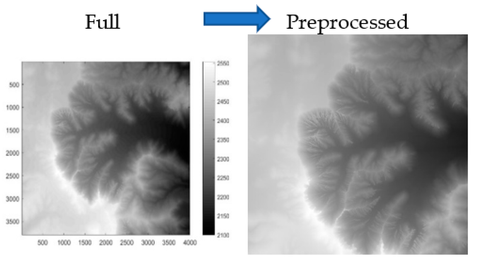
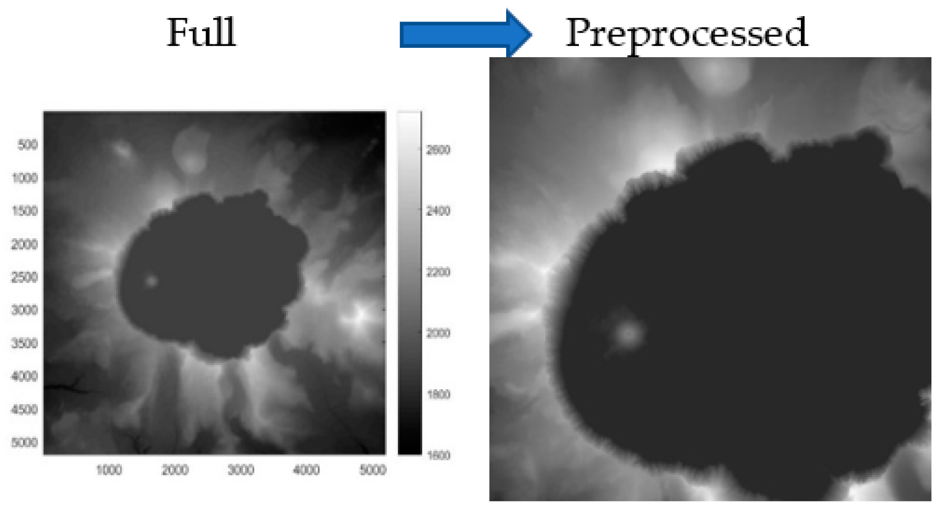
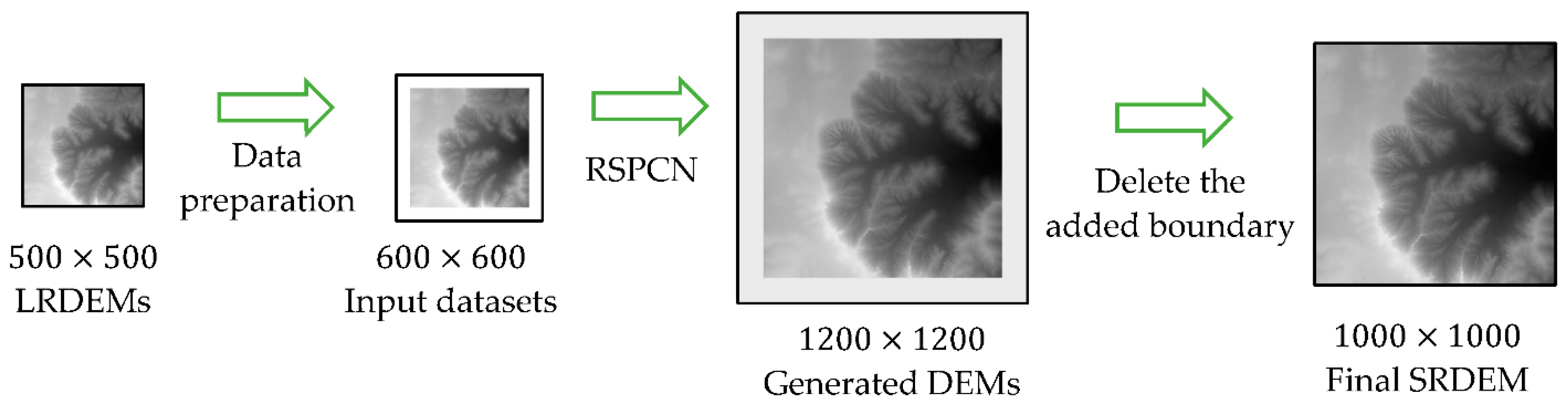
4.1. Adding-“Zero” Data Preprocessing Method

During the convolutional layers, the boundary pixels of the DEMs cannot be convoluted. The reason is that the boundary pixels cannot completely overlap the convolution kernel. For example, the edge of one pixel will not be processed with a kernel 3 × 3. Therefore, we add “zero” (representing value = 255 in the gray picture) to the boundary of the DEMs. In the results, we will delete the “zero” boundary of the generated DEMs and finally obtain the SRDEMs to do the comparison and analysis. The specific data processing steps are as follows.

Firstly, we add “zero” to the boundary of the 500 × 500 LRDEMs to build 600 × 600 LRDEMs as the training datasets. Then, after the training process, we obtain 1200 × 1200 generated DEMs. Finally, we obtain the final 1000 × 1000 SRDEMs by deleting the boundary. The whole process are shown in Figure 10. By comparing with the preprocessed 1000 × 1000 DEMs, which are shown in Figure 1, Figure 2, Figure 3, Figure 4 and Figure 5, the accuracy of the final 1000 × 1000 SRDEMs is analyzed. The experimental environment is a modest laptop computer (a 64-bit AMD Ryzen 54,600U with Radeon Graphics @ 2.10 GHz, RAM 16 GB). Visual Studio 2015 and Opencv 3.1.0 are used to transform the normalized data into binary data that is trained in the Tensorflow platform.

4.2. Data Augmentation (DA)

During the experimental process, the input datasets we use are different types of the LRDEMs, divided into six types (0 to 5), and the training datasets are HRDEMs derived from 3DEP. The training datasets have only one DEM per type. Thus, in order to alleviate the effect of over-fitting problems and expand the training datasets, we use the data augmentation (DA) method [66] to expand them. The detailed step is adding 100 times of Gaussian noise $\epsilon ~ N\left(0,∆d\right)$ into each type of the DEM, where $∆d$ means the resolution of the LRDEMs. Thus, we obtain 100 DEMs per type and 600 DEMs in total; test samples contain merely six DEMs in total, with 1 DEM per type.

4.3. Selection of Training DataSets

Through the above steps, we have two ways to generate training datasets.

Training datasets No. 1: six types with 100 DEMs of each type (by DA).

Training datasets No. 2: six types with 1 DEM of each type.

The results are compared and analyzed by two different types of training datasets. As for the evaluation indexes of the experiments, root mean square error (RMSE) [67,68], peak signal to noise ratio (PSNR) and structural similarity (SSIM) [69] are used. The smaller the RMSE is, the higher the accuracy of the DEM super-resolution is, as shown in Formula (3). The bigger the PSNR is, the more similar the super-resolution DEM is to the real DEM data, as is shown in Formulas (4) and (5). SSIM is another index to measure the similarity of two images, which is modeled as a combination of brightness, contrast and structure. The value of SSIM is in the range of −1 to 1. The closer the SSIM is to 1, the more similar the super-resolution DEM is to the real DEM data, as shown in Formulas (6)–(8) [69].

$$RMSE=\sqrt{\frac{1}{n^2}{\displaystyle \sum }_{i=1}^n{\displaystyle \sum }_{j=1}^n{\Vert \mathit{x}\left(i,j\right)-\mathit{y}\left(i,j\right)\Vert }^2} , \left(i=0,1,\cdots \right)$$

(3)

$$PSNR=10\times {\log }_{10}\left(\frac{{\left(2^p-1\right)}^2}{MSE}\right)$$

(4)

$$MSE=\frac{1}{n^2}{\displaystyle \sum }_{i=1}^n{\displaystyle \sum }_{j=1}^n{\Vert \mathit{x}\left(i,j\right)-\mathit{y}\left(i,j\right)\Vert }^2=RMS{E}^2$$

(5)

$$SSIM\left(\mathit{x},\mathit{y}\right)=\frac{\left(2{\mu }_x{\mu }_y+c_1\right)\left(2{\sigma }_{xy}+c_2\right)}{\left({\mu }_x{}^2+{\mu }_y{}^2+c_1\right)\left(\left({\sigma }_x{}^2+{\sigma }_y{}^2+c_2\right)\right)}$$

(6)

$$c_1={\left(k_{1}L\right)}^2, k_1=0.01$$

(7)

$$c_2={\left(k_{2}L\right)}^2, k_1=0.03$$

(8)

In the above formulas, $\mathit{x}$ is normalized 1000$\times$1000 DEM data (shown in Figure 1, Figure 2, Figure 3, Figure 4 and Figure 5), and $\mathit{y}$ is normalized final SRDEM data. In Formula (4), $p$ is the number of bits for each sample value, and MSE is the mean square error, as shown in Formula (5). In Formula (6)–(8), ${\mu }_{\mathit{x}},{\mu }_{\mathit{y}}$ are the mean of $\mathit{x}$ and $\mathit{y}$, respectively; ${\sigma }_{\mathit{x}}, {\sigma }_{\mathit{y}}$ are the standard deviation of $\mathit{x}$ and $\mathit{y}$, respectively; ${\sigma }_{\mathit{x}\mathit{y}}$ is the covariance of $\mathit{x}$ and $\mathit{y}$; and $c_1, c_2$ are fixed parameters used to maintain the stability of Formula (6), where $L$ is the maximum value of the pixel (in this paper, $L\approx 1$, due to normalization).

We compare the different selections of Adam’s initial learning rate value ($\delta =0.01, 0.001, 0.0001$) using two types of training datasets (No.1 and No.2), respectively, as shown in

Table 2. Evaluation index of SR-DEM with different $\delta$ using No. 1 training datasets $\left(m=100\right)$.

	Terrain	Bryce Canyon	Crater Lake	Great Sand Dunes	Jackson Hole	Kilauea	Sand Hills
Evaluation Index
RMSE	$\delta =0.01$	5.50991	8.62677	7.90989	1.35980	8.84151	2.41966
	$\delta =0.001$	4.69826	9.04652	5.33902	1.11628	6.52938	2.07646
	$\delta =0.0001$	4.22736	7.85174	5.20805	1.01796	5.74747	1.75736
PSNR (dB)	$\delta =0.01$	64.2114	65.2327	71.8701	66.8205	64.7547	65.748
	$\delta =0.001$	66.9796	64.4074	78.6985	70.2485	70.021	68.4052
	$\delta =0.0001$	68.8144	66.8681	79.13	71.8502	72.2368	71.3037
SSIM	$\delta =0.01$	0.997758	0.998038	0.999808	0.999277	0.997903	0.998126
	$\delta =0.001$	0.999453	0.997431	1.00022	1.00034	1.00002	0.999266
	$\delta =0.0001$	1.00009	0.998964	1.00025	1.00063	1.00038	0.999936

and

Table 3. Evaluation index of SR-DEM with different $\delta$ using No. 2 training datasets ($m=500$ ).

	Terrain	Bryce Canyon	Crater Lake	Great Sand Dunes	Jackson Hole	Kilauea	Sand Hills
Evaluation Index
RMSE (m)	$\delta =0.01$	4.87827	8.65312	5.22679	1.12233	5.41871	2.16812
	$\delta =0.001$	4.75129	8.54755	5.08283	1.01830	5.35660	2.10352
	$\delta =0.0001$	4.58169	7.74609	4.753035	0.99737	4.77073	1.98041
PSNR (dB)	$\delta =0.01$	66.3266	65.1797	79.0675	70.1546	73.26	67.6548
	$\delta =0.001$	66.7847	65.393	79.5527	71.8444	73.4602	68.1802
	$\delta =0.0001$	67.4161	67.1034	80.7181	72.2052	75.4724	69.2279
SSIM	$\delta =0.01$	0.999143	0.998001	1.00023	1.00032	1.00051	0.999007
	$\delta =0.001$	0.999393	0.99816	1.00024	1.00063	1.00051	0.999196
	$\delta =0.0001$	0.999606	0.999054	1.00027	1.00068	1.00066	0.999496

, where $m$ denotes the number of training steps.

The results show that the parameter $\delta$ is chosen as 0.0001 for both training datasets, making the algorithm converge faster. Then, extensive experiments are conducted at the same training steps (500) for both training datasets. The results are shown in

Table 4. Evaluation index of SR-DEM with different types of training datasets ($m=500, \delta =0.0001$).

	Terrain	Bryce Canyon	Crater Lake	Great Sand Dunes	Jackson Hole	Kilauea	Sand Hills
Evaluation Index
RMSE (Meter)	No.1 type	4.73405	8.93722	5.46223	1.11783	4.99111	2.14315
	No.2 type	4.58169	7.74609	4.75304	0.99737	4.77073	1.98041
PSNR (dB)	No.1 type	66.8479	64.6185	78.3022	70.2244	74.6879	67.856
	No.2 type	67.4161	67.1034	80.7181	72.2052	75.4724	69.2279
SSIM	No.1 type	0.99941	0.997578	1.00021	1.00033	1.00061	0.999084
	No.2 type	0.99961	0.999054	1.00027	1.00068	1.00066	0.999496

.

It can be seen from Table 4 that different training datasets have different effects on different types of landforms. Compared with the No. 1 training datasets, the training No. 2 datasets perform better, with the highest PSNR and the smallest RMSE. However, it has the disadvantage of instability, as shown in Figure 11. When the Adam’s initial learning rate is not that good (for example, $\delta =0.01$ in Figure 11), the No.2 training datasets make the algorithm unstable. When the training steps are close to 100 steps, the cost values become oscillating from 2.0166$\times {10}^{-4}$ (the 91st step) back to 0.02023 (the 99th step).

When the chosen Adam’s initial learning rate $\delta$ is unsuitable, we use No. 1 training datasets with the DA process to increase the stability and accuracy of the algorithm. When the selected parameter $\delta$ makes the algorithm converge in an efficient way (such as $\delta =0.0001$ in Table 3), the No. 2 training datasets could be chosen to reduce the training time consumption. Thus, we choose the experiment with No. 2 training datasets and $\delta =0.0001$. With the number of training steps set up as 10,000, the loss function curves of the model in the training process are shown in Figure 12, showing that the loss function is fast converging. During the training process, the cost goes down from $5.8823\times {10}^{-3}$ to $5.2325\times {10}^{-5}$. After about 400 training steps, the network finds the distribution characteristics of the terrain by deep learning.

5. Comparison and Analysis

5.1. Results Based on ESPCN

In this section, we use No. 2 datasets with $\delta =0.0001$ to generate HRDEMs. After 10,000 training steps, compared with traditional interpolation methods (bicubic, nearest-neighbor, bilinear), the accuracy of different methods is shown in

Table 5. Accuracy of SR-DEM with different methods.

	Methods	Bicubic	Nearest-Neighbor	Bilinear	ESPCN
Evaluation Index
PSNR (dB)	Bryce Canyon	71.8991	72.0109	71.984	88.8061
	Crater Lake	67.209	67.216	67.2109	83.3836
	Great Sand Dunes	80.3492	80.5908	80.5498	87.5361
	Jackson Hole	78.3517	78.2049	78.1226	80.088
	Kilauea	96.5075	97.952	96.7137	91.5163
	Sand Hills	76.0127	76.1237	75.9362	84.1242
SSIM	Bryce Canyon	1.00101	1.00104	1.00103	1.00138
	Crater Lake	0.99942	0.999418	0.999419	1.00106
	Great Sand Dunes	1.0004	1.00041	1.0004	1.00033
	Jackson Hole	1.00126	1.00125	1.00125	1.0012
	Kilauea	1.00095	1.00095	1.00095	1.00092
	Sand Hills	1.00054	1.00054	1.00053	1.00062
RMSE (m)	Bryce Canyon	3.53958	3.51686	3.52232	1.33745
	Crater Lake	7.69915	7.69601	7.69827	3.03441
	Great Sand Dunes	4.85507	4.78801	4.79932	3.21012
	Jackson Hole	0.70015	0.706093	0.70945	0.63356
	Kilauea	1.421371	1.30796	1.40460	1.89448
	Sand Hills	1.340098	1.33156	1.34601	0.84014

.

According to Table 5, it can be seen that the RSPCN method performs better when facing different terrain types than the other traditional interpolation algorithms, with more PSNR values higher and more RMSE values smaller. As for Kilauea (shield caldera), although the PSNR and RMSE values are not the best, those of our method are very close to the best ones. These four methods all perform well regarding the SSIM index (close to 1). As for the bicubic interpolation method, the PSNR and RMSE values of the Jackson Hole DEM data perform best among the three traditional methods. As for the nearest-neighbor interpolation method, the PSNR and RMSE values perform better except for Jackson Hole than those of the other two traditional methods. As for the bilinear interpolation method, its results are similar to those of the bicubic interpolation method, but it does not perform well for Jackson Hole DEM data and Sand Hills DEM data. However, the evaluation index values of the three traditional methods are very close to each other and only have slight differences. The accuracy of the RSPCN model becomes higher every step during the training process, while other traditional interpolation methods could not improve the precision by learning. Therefore, the RSPCN algorithm has some advantages in improving the accuracy of the DEM interpolation. The error maps of the generated SRDEMs of different terrain types are shown in Figure 13. For each test site, the color bar scaling of the errors is the same among different methods. From Figure 13, compared with other methods, it can be seen that our method has smaller maximum error values except for the Kīlauea terrain, which could effectively reconstruct the SRDEMs.

5.2. Results Based on RSPCN

Based on the proposed RSPCN method in Section 3.2, we use 62$\times$ 62 LRDEMs to build 992$\times$992 HRDEMs by setting the magnification factor $N=4$ ($2^N=\frac{992}{62}$). We choose the dataset eroded plateau (Bryce Canyon, UT, USA), as shown in Figure 1. Firstly, we add “zero” to the boundary of the 62$\times$62 LRDEMs and generate 75$\times$75 experimental DEMs to generate 1200$\times$1200 HRDEMs. After the training process, we delete the boundary and finally obtain the 992$\times$992 SRDEMs. The accuracy of RSCPN is shown in

Table 6. Accuracy of RSPCN with different methods.

	Methods	PSNR (dB)	SSIM	RMSE (m)
Evaluation Index
RSPCN	Bryce Canyon	68.7828	1.00012	4.23506

. After 10,000 training steps, the process of the RSPCN and the loss function curves are shown in Figure 14 and Figure 15.

6. Discussion

As an important expression model of topography, DEM has been applied to the dynamic simulation of ground surface, multi-scale modeling in geoscience, and other related fields. The DEM interpolation method makes a prediction of the values of a primary variable at scattered data within the same sampled area [70,71], which is an important way to build a spatially continuous surface by DEM data.

At present, most common solutions for spatial interpolation focus on geostatistical methods. In 1951, D.G. Krige [72] presented a linear least squares regression interpolation method, the Kriging interpolation method. In the 1960s, Birkhoff and Garabdian [73] proposed the two-dimensional spline function, and De Boor [74] introduced bicubic spline interpolation. Spline interpolation could better fit the overall trend of the surface but ignored the detailed information of the terrain. In 1964, Bengtsson and Nordbeck [75] proposed a vector-based method, triangulated irregular network (TIN). TIN can reduce the redundancy of flat areas and can represent topographic linear features well. The research on TIN has not stopped [76,77,78,79]. However, TINs ignore non-linear information and are unable to represent spatial terrain types, such as cliffs, caves or holes. In 1968, Shepard [80] proposed the inverse distance weighting (IDW) method. IDW is simple and fast to calculate, but it fails to incorporate the spatial structure and ignores information beyond the neighborhood.

Among these common interpolation methods, the Kriging suite has been proven to perform better in most of the DEM modeling with high geometric accuracy and has become the most common method used in spatial interpolation. However, the goals of Kriging are practically unattainable since the mean error and the variance of the errors are always unknown [71]. Meanwhile, we use the Kriging algorithm programmed in MATLAB software to deal with the 1000 × 1000 DEM array on the same computational environment described in Section 4. The program exceeds the maximum array size preference in the current computational environment. This shows that compared with our method, the Kriging method is more computationally intensive.

Entering the 21st century, researchers also explored other theories to interpolate the DEM. Based on the fractal geometry theory, Paramanathan P. and Uthayakumar R. [81], Jiang P., et al. [82] and Liu L. and Wang X., et al. [83] have developed the fractal interpolation method, which eliminates smoothing problems. However, it could be only used in regular grid data. Based on the surface theory and differential geometry theory, Yue [71] presents the high accuracy surface modeling (HASM) method to simulate the Earth’s surface system, which has been proven to perform well in eco-environmental surface modeling. Based on the deep learning theory, the “super-resolution” theory is commonly used in the image processing field. When it comes to DEM construction, our RSPCN method presents a deep-learning-based solution for spatial interpolation with higher accuracy than that of the traditional linear interpolation methods. In order to express the comparison between our method and the traditional method more intuitively, we have carried out a pixel-level comparison, the result of which is attached as Supplementary Material. Moreover, the paper provides a whole set of data processing steps from the preprocessing of raw terrain datasets to the final output. The simple codes make our method well-suited for various data formats.

7. Conclusions

In this paper, we introduce and improve the ESPCN method. Then, based on the recursion theory, we propose the recursive sub-pixel convolutional neural networks (RSPCN) method. The experimental datasets are six archetypal landform datasets derived from 3DEP LiDAR sources, which have typical terrain characteristics, including an eroded plateau, a volcanic caldera, active sand dunes, a braided riverbed, a shield caldera, and stabilized sand dunes. Except for the shield caldera, the results of the SR by RSPCN are better than the other traditional linear interpolation methods.

Our model could predict the terrain information of unmeasured points and be close to the real terrain information with relatively high fidelity to the real terrain structures. Compared with the traditional linear interpolation methods, the RSPCN method could effectively learn the probability distribution characteristics of the terrain, which could better balance the local characteristics and the overall characteristics. After extensive experiments, except for the shield caldera terrain, our method performs better than bilinear interpolation, bicubic interpolation, and nearest neighbor interpolation. Compared with the classic image super-resolution method based on deep learning, SRCNN, the RSPCN method directly processes on the sub-pixel level, decreasing the amount of computation. Compared with the ESPCN method, the RSPCN method introduces recursive ideas to shorten the depth of the network.

Meanwhile, we present a data preprocessing method by adding “zero” to the boundary of input DEM data, which improves the RSPCN method’s accuracy and convergence. We believe that this adding “zero” method provides an available data preprocessing method in the CNN-based interpolation field. Further addressing and analyzing the effects of the various data preprocessing methods is another focus of our future work. Finally, as an alternative to other deep learning methods, the RSPCN method further explores the application of deep learning models in the field of DEM modeling.

References

1. Miller, C.L.; Laflamme, R.A. The digital terrain model-theory and application. Photogramm. Eng. 1958, 24, 433–442. [Google Scholar]
2. Guoan, T.; Fayuan, L.; Xuejun, L. Digital Elevation Model Course; Science Press: Beijing, China, 2010. [Google Scholar]
3. Tang, G.A.; Fa-Yuan, L.I.; Xiong, L.Y. Progress of Digital Terrain Analysis in the Loess Plateau of China. Geogr. GeoInf. Sci. 2017, 33, 1–7. [Google Scholar]
4. Kubade, A.; Sharma, A.; Rajan, K.S. Feedback Neural Network Based Super-Resolution of DEM for Generating High Fidelity Features. In Proceedings of the IGARSS 2020—2020 IEEE International Geoscience and Remote Sensing Symposium, Virtual Symposium, Waikoloa, HI, USA, 26 September–2 October 2020; pp. 1671–1674. [Google Scholar]
5. Kubade, A.; Patel, D.; Sharma, A.; Rajan, K.S. AFN: Attentional Feedback Network Based 3D Terrain Super-Resolution. In Proceedings of the 15th Asian Conference on Computer Vision (ACCV2020), Kyoto, Japan, 30 November–4 December 2020. [Google Scholar]
6. Argudo, O.; Chica, A.; Andujar, C. Terrain Super-resolution through Aerial Imagery and Fully Convolutional Networks. Comput. Graph. Forum 2018, 37, 101–110. [Google Scholar] [CrossRef]
7. Cheol, S.P.; Min, K.P.; Moon, G.K. Super-resolution image reconstruction: A technical overview. IEEE Signal Process. Mag. 2003, 20, 21–36. [Google Scholar]
8. Shen, H.; Peng, L.; Yue, L.; Yuan, Q.; Zhang, L. Adaptive Norm Selection for Regularized Image Restoration and Super-Resolution. IEEE Trans. Cybern. 2016, 46, 1388–1399. [Google Scholar] [CrossRef]
9. Farsiu, S. A Fast and Robust Framework for Image Fusion and Enhancement. Ph.D. Dissertation, University of California, Santa Cruz, CA, USA, December 2015. [Google Scholar]
10. Walt, S. Super-Resolution Imaging; CRC Press: Boca Raton, FL, USA, 2010. [Google Scholar]
11. Tan, B.; Xing, S.; Xu, Q.; Li, J.-S. A Research on SPOT5 Supermode Image Processing. Remote Sens. Technol. Appl. 2004, 19, 249–252. [Google Scholar]
12. Li, L.; Wang, W.; Luo, H.; Ying, S. Super-Resolution Reconstruction of High-Resolution Satellite ZY-3 TLC Images. Sensors 2017, 17, 1062. [Google Scholar] [CrossRef] [PubMed] [Green Version]
13. Tsai, R.Y.; Huang, T.S. Multiframe image restoration and registration. In Advances in Computer Vision and Image Processing; JAI Press, Inc.: Greenwich, CT, USA, 1984; Volume 1. [Google Scholar]
14. Yue, T.-X.; Du, Z.-P.; Song, D.-J.; Gong, Y. A new method of surface modeling and its application to DEM construction. Geomorphology 2007, 91, 161–172. [Google Scholar] [CrossRef]
15. Chen, C.; Yue, T. A method of DEM construction and related error analysis. Comput. Geosci. 2010, 36, 717–725. [Google Scholar] [CrossRef]
16. Yue, T.-X. Progress in earth surface modeling. J. Remote Sens. 2011, 15, 1105–1124. [Google Scholar]
17. Wang, C.; Tang, G.; Liu, X.; Tao, Y. The model of terrain features preserved in grid DEM. Geomat. Inf. Sci. Wuhan Univ. 2009, 34, 1149–1154. [Google Scholar]
18. Yiping, G. Research on the DEM Modeling Methods of Plain River Network Area; Nanjing Normal University: Nanjing, China, 2010. [Google Scholar]
19. Chen, Z.; Wang, X.; Xu, Z.; Wenguang, H. Convolutional Neural Network Based Dem Super Resolution. In ISPRS—International Archives of the Photogrammetry, Remote Sensing and Spatial Information Sciences, Proceedings of the XXIII ISPRS Congress, Prague, Czech Republic, 12–19 July 2016; ISPRS: Hannover, Germany, 2016; pp. 247–250. [Google Scholar]
20. Yue, L.; Shen, H.; Yuan, Q.; Zhang, L. Fusion of multi-scale DEMs using a regularized super-resolution method. Int. J. Geogr. Inf. Sci. 2015, 29, 2095–2120. [Google Scholar] [CrossRef]
21. Liu, X. Airborne LiDAR for DEM generation: Some critical issues. Prog. Phys. Geogr. Earth Environ. 2008, 32, 31–49. [Google Scholar] [CrossRef]
22. Xu, Z.; Wang, X.; Chen, Z.; Xiong, D.; Ding, M.; Hou, W. Nonlocal similarity based DEM super resolution. ISPRS J. Photogramm. Remote Sens. 2015, 110, 48–54. [Google Scholar] [CrossRef]
23. Jiayao, W. Principles of Spatial Information System; Science Press: Beijing, China, 2001. [Google Scholar]
24. Gao, J. Construction of Regular Grid DEMs from Digitized Contour Lines: A Comparative Study of Three Interpolators. Ann. GIS 2001, 7, 8–15. [Google Scholar] [CrossRef]
25. Lam, N.S.-N. Spatial Interpolation Methods: A Review. Am. Cartogr. 1983, 10, 129–149. [Google Scholar] [CrossRef]
26. Declercq, F.A.N. Interpolation Methods for Scattered Sample Data: Accuracy, Spatial Patterns, Processing Time. Cartogr. Geogr. Inf. Syst. 1996, 23, 128–144. [Google Scholar] [CrossRef]
27. Rajan, D.; Chaudhuri, S. Generalized interpolation and its application in super-resolution imaging. Image Vis. Comput. 2001, 19, 957–969. [Google Scholar] [CrossRef]
28. Capel, D. Image Mosaicing and Super-Resolution (Cphc/Bcs Distinguished Dissertations.); Springer: London, UK, 2004. [Google Scholar]
29. Zhao, X.Y.; Su, Y.; Dong, Y.Q.; Wang, J.M.; Zhai, L.P. Kind of super-resolution method of CCD image based on wavelet and bicubic interpolation. Appl. Res. Comput. 2009, 26, 2365–2367. [Google Scholar]
30. Tong, C.S.; Leung, K.T. Super-resolution reconstruction based on linear interpolation of wavelet coefficients. Multidimens. Syst. Signal Process. 2007, 18, 153–171. [Google Scholar] [CrossRef]
31. Aguilar, F.J.; Agüera, F.; Aguilar, M.A.; Carvajal-Ramírez, F. Effects of Terrain Morphology, Sampling Density, and Interpolation Methods on Grid DEM Accuracy. Photogramm. Eng. Remote Sens. 2005, 71, 805–816. [Google Scholar] [CrossRef] [Green Version]
32. Zhou, W.; Bovik, A.C.; Sheikh, H.R.; Simoncelli, E.P. Image quality assessment: From error visibility to structural similarity. IEEE Trans. Image Process. 2004, 13, 600–612. [Google Scholar]
33. Wang, Y.; Zhu, C.; Shi, W. Application of B Spline and Smoothing Spline on Interpolating the DEM Based on Rectangular Grid. Acta Geod. Cartogr. Sin. 2000, 29, 240–244. [Google Scholar]
34. Wang, Y.G.; Zhu, C.Q.; Wang, Z.W. A Surface Model of Grid DEM Based on Coons Surface. Acta Geod. Cartogr. Sin. 2008, 37, 217–222. [Google Scholar]
35. Chen, C. Grid-Based DEM Construction by Means of Coons Patch. J. Geod. Geodyn. 2012, 32, 87–98. [Google Scholar]
36. Hardy, R.L. Multiquadric equations of topography and other irregular surfaces. J. Geophys. Res. Space Phys. 1971, 76, 1905–1915. [Google Scholar] [CrossRef]
37. Franke, R. Scattered data interpolation: Tests of some methods. Math. Comp. 1982, 38, 181–200. [Google Scholar]
38. Foley, T.A. Interpolation and approximation of 3-D and 4-D scattered data. Comput. Math. Appl. 1987, 13, 711–740. [Google Scholar] [CrossRef] [Green Version]
39. Jichun, L.; Chen, C.S. A simple efficient algorithm for interpolation between different grids in both 2D and 3D. Math. Comput. Simul. 2002, 58, 125–132. [Google Scholar]
40. Rippa, S. An algorithm for selecting a good value for the parameter c in radial basis function interpolation. Adv. Comput. Math. 1999, 11, 193–210. [Google Scholar] [CrossRef]
41. Tao, H.; Tang, X.; Liu, J.; Tian, J. Superresolution remote sensing image processing algorithm based on wavelet transform and interpolation. In Image Processing and Pattern Recognition in Remote Sensing, Proceedings of the Third International Asia-Pacific Environmental Remote Sensing Remote Sensing of the Atmosphere, Ocean, Environment, and Space, Hangzhou, China, 23–27 October 2002; Ungar, S.G., Mao, S., Yasuoka, Y., Eds.; SPIE: Bellingham, WA, USA, 2003; Volume 4898, pp. 259–264. [Google Scholar] [CrossRef]
42. Lertrattanapanich, S.; Bose, N.K. High resolution image formation from low resolution frames using delaunay triangulation. IEEE Trans. Image Process. 2002, 11, 1427–1441. [Google Scholar] [CrossRef]
43. Sanchez-Beato, A.; Pajares, G. Noniterative Interpolation-Based Super-Resolution Minimizing Aliasing in the Reconstructed Image. IEEE Trans. Image Process. 2008, 17, 1817–1826. [Google Scholar] [CrossRef]
44. Chao, D.; Loy, C.C.; He, K.; Tang, X. Learning a Deep Convolutional Network for Image Super-Resolution. In Proceedings of the 13th European Conference on Computer Vision (ECCV), Zurich, Switzerland, 6–12 September 2014. [Google Scholar]
45. Irani, M.; Peleg, S. Super resolution from image sequences. In Proceedings of the 10th International Conference on Pattern Recognition, Atlantic City, NJ, USA, 16–21 June 1990; Volume 2, pp. 115–120. [Google Scholar]
46. Tom, B.C.; Katsaggelos, A.K. Reconstruction of a high-resolution image by simultaneous registration, restoration, and interpolation of low-resolution images. In Proceedings of the International Conference on Image Processing, Washington, DC, USA, 23–26 October 1995; Volume 2, p. 2539. [Google Scholar]
47. Shen, H.; Zhang, L.; Huang, B.; Li, P. A MAP Approach for Joint Motion Estimation, Segmentation, and Super Resolution. IEEE Trans. Image Process. 2007, 16, 479–490. [Google Scholar] [CrossRef]
48. Hardie, R.C.; Barnard, K.J.; Armstrong, E.E. Joint MAP registration and high-resolution image estimation using a sequence of undersampled images. IEEE Trans. Image Process. 1997, 6, 1621–1633. [Google Scholar] [CrossRef] [Green Version]
49. Yang, J.; Wang, Z.; Lin, Z.; Cohen, S.; Huang, T.S. Coupled Dictionary Training for Image Super-Resolution. IEEE Trans. Image Process. 2012, 21, 3467–3478. [Google Scholar] [CrossRef] [PubMed]
50. Ni, K.S.; Nguyen, T.Q. Image Superresolution Using Support Vector Regression. IEEE Trans. Image Process. 2007, 16, 1596–1610. [Google Scholar] [CrossRef]
51. Hayat, K. Super-Resolution via Deep Learning. Research Gate. 2017. Available online: https://www.researchgate.net/publication/318009713_Super-Resolution_via_Deep_Learning (accessed on 5 July 2017).
52. Linyang, H. Research on Key Techniques of Super-resolution Reconstruction of Aerial Images; Changchun Institute of Optics, Fine Mechanics and Physics: Changchun, China, 2016. [Google Scholar]
53. Dong, C.; Loy, C.C.; He, K.; Tang, X. Image Super-Resolution Using Deep Convolutional Networks. IEEE Trans. Pattern Anal. Mach. Intell. 2015, 38, 295–307. [Google Scholar] [CrossRef] [PubMed] [Green Version]
54. Yang, J.W.; Huang, T.; Ma, Y.J. Image Super-Resolution Via Sparse Representation. IEEE Trans. Image Process. 2010, 19, 2861–2873. [Google Scholar] [CrossRef] [PubMed]
55. Aharon, M.; Elad, M.; Bruckstein, A. K-SVD: An Algorithm for Designing Overcomplete Dictionaries for Sparse Representation. IEEE Trans. Signal Process. 2006, 54, 4311–4322. [Google Scholar] [CrossRef]
56. Shin, D.; Spittle, S. LoGSRN: Deep Super Resolution Network for Digital Elevation Model. In Proceedings of the 2019 IEEE International Conference on Systems, Man and Cybernetics (SMC), Bari, Italy, 6–9 October 2019; pp. 3060–3065. [Google Scholar]
57. Dong, C.; Loy, C.C.; Tang, X. Accelerating the Super-Resolution Convolutional Neural Network. In Proceedings of the European Conference on Computer Vision, Amsterdam, The Netherlands, 11–14 October 2016. [Google Scholar]
58. Zeiler, M.; Fergus, R. Visualizing and Understanding Convolutional Networks. In Proceedings of the 13th European Conference on Computer Vision (ECCV), Zurich, Switzerland, 6–12 September 2014. [Google Scholar]
59. Shi, W.; Caballero, J.; Huszar, F.; Totz, J.; Aitken, A.P.; Bishop, R.; Rueckert, D.; Wang, Z. Real-Time Single Image and Video Super-Resolution Using an Efficient Sub-Pixel Convolutional Neural Network. In Proceedings of the 2016 IEEE Conference on Computer Vision and Pattern Recognition (CVPR), Las Vegas, NV, USA, 27–30 June 2016; pp. 1874–1883. [Google Scholar]
60. Kim, J.; Lee, J.K.; Lee, K.M. Deeply-Recursive Convolutional Network for Image Super-Resolution. In Proceedings of the 2016 IEEE Conference on Computer Vision and Pattern Recognition (CVPR), Las Vegas, NV, USA, 27–30 June 2016. [Google Scholar]
61. Lim, B.; Son, S.; Kim, H.; Nah, S.; Lee, K.M. Enhanced Deep Residual Networks for Single Image Super-Resolution. In Proceedings of the 2017 IEEE Conference on Computer Vision and Pattern Recognition Workshops (CVPRW), Honolulu, HI, USA, 21–26 July 2017; pp. 1132–1140. [Google Scholar]
62. Qin, M.; Hu, L.; Du, Z.; Gao, Y.; Qin, L.; Zhang, F.; Liu, R. Achieving Higher Resolution Lake Area from Remote Sensing Images Through an Unsupervised Deep Learning Super-Resolution Method. Remote Sens. 2020, 12, 1937. [Google Scholar] [CrossRef]
63. Jiao, D.; Wang, D.; Lv, H.; Peng, Y. Super-resolution reconstruction of a digital elevation model based on a deep residual network. Open Geosci. 2020, 12, 1369–1382. [Google Scholar] [CrossRef]
64. Kennelly, P.J.; Patterson, T.; Jenny, B.; Huffman, D.P.; Marston, B.E.; Bell, S.; Tait, A.M. Elevation models for reproducible evaluation of terrain representation. Cartogr. Geogr. Inf. Sci. 2021, 48, 63–77. [Google Scholar] [CrossRef]
65. Kingma, D.P.; Ba, J. Adam: A method for Stochastic Optimization. Computer Science. arXiv 2014, arXiv:1412.6980v9. [Google Scholar]
66. Van Dyk, D.A.; Meng, X.-L. The Art of Data Augmentation. J. Comput. Graph. Stat. 2001, 10. [Google Scholar] [CrossRef]
67. Chai, T.; Draxler, R.R. Root mean square error (RMSE) or mean absolute error (MAE)?—Arguments against avoiding RMSE in the literature. Geosci. Model Dev. 2014, 7, 1247–1250. [Google Scholar] [CrossRef] [Green Version]
68. Sepasgozar, S.M.E.; Forsythe, P.; Shirowzhan, S. Evaluation of Terrestrial and Mobile Scanner Technologies for Part-Built Information Modeling. J. Constr. Eng. Manag. 2018, 144. [Google Scholar] [CrossRef]
69. Wang, Z.; Bovik, A.C. A universal image quality index. IEEE Signal Process. Lett. 2002, 9, 81–84. [Google Scholar] [CrossRef]
70. Li, J.; Heap, A.D. Spatial interpolation methods applied in the environmental sciences: A review. Environ. Model. Softw. 2014, 53, 173–189. [Google Scholar] [CrossRef]
71. Yue, T.; Zhao, N.; Liu, Y.; Wang, Y.; Zhang, B.; Du, Z.; Fan, Z.; Shi, W.; Chen, C.; Zhao, M.; et al. A fundamental theorem for eco-environmental surface modelling and its applications. Sci. China Earth Sci. 2020, 63, 1092–1112. [Google Scholar] [CrossRef]
72. Krige, D.G. A statistical approach to some basic mine valuation problems on the Witwatersrand. J. South Afr. Inst. Min. Metall. 1951, 52, 119–139. [Google Scholar]
73. Birkhoff, G.; Garabedian, H.L. Smooth Surface Interpolation. J. Math. Phys. 1960, 39, 258–268. [Google Scholar] [CrossRef]
74. Boor, C.D. Bicubic Spline Interpolation. J. Math. Phys. 1962, 41, 212–218. [Google Scholar] [CrossRef]
75. Bengtsson, B.-E.; Nordbeck, S. Construction of isarithms and isarithmic maps by computers. BIT Numer. Math. 1964, 4, 87–105. [Google Scholar] [CrossRef]
76. Tse, R.O.; Gold, C. TIN meets CAD—extending the TIN concept in GIS. Futur. Gener. Comput. Syst. 2004, 20, 1171–1184. [Google Scholar] [CrossRef]
77. Bartholdi, J.J.; Goldsman, P. The vertex-adjacency dual of a triangulated irregular network has a Hamiltonian cycle. Oper. Res. Lett. 2004, 32, 304–308. [Google Scholar] [CrossRef]
78. Tucker, G.E.; Lancaster, S.T.; Gasparini, N.M.; Bras, R.F.; Rybarczyk, S.M. An object-oriented framework for distributed hydrologic and geomorphic modeling using tri-angulated irregular networks. Comput. Geosci. 2001, 27, 959–973. [Google Scholar] [CrossRef]
79. Kumler, M.P.; Goodchild, M.F. New Technique for Selecting the Vertices for a TIN and a Comparison of TINs and DEMs over a Variety of Surfaces. 1991. Available online: https://0-asu-pure-elsevier-com.brum.beds.ac.uk/en/publications/new-technique-for-selecting-the-vertices-for-a-tin-and-a-comparis (accessed on 1 January 1991).
80. Shepard, D. A two-dimensional interpolation function for irregularly-spaced data. In Proceedings of the 1968 23rd ACM National Conference, New York, NY, USA, 27–29 August 1968; pp. 517–524. [Google Scholar]
81. Paramanathan, P.; Uthayakumar, R. Fractal interpolation on the Koch Curve. Comput. Math. Appl. 2010, 59, 3229–3233. [Google Scholar] [CrossRef] [Green Version]
82. Jiang, P.; Liu, F.; Wang, J.; Song, Y. Cuckoo search-designated fractal interpolation functions with winner combination for estimating missing values in time series. Appl. Math. Model. 2016, 40, 9692–9718. [Google Scholar] [CrossRef]
83. Liu, L.; Wang, X.; Ren, H. 3D Seabed Terrain Establishment Based on Moving Fractal Interpolation. In Proceedings of the 2014 Seventh International Joint Conference on Computational Sciences and Optimization, Beijing, China, 4–6 July 2014; pp. 6–10. [Google Scholar]
Figure 1. Eroded plateau (Bryce Canyon, UT, USA) [64]: 1000 × 1000 with pixel size of 3 m.
Ijgi 10 00501 g001
Figure 2. Volcanic caldera (Crater Lake, OR, USA) [64]: 1000 × 1000 with pixel size of 9.99 m.
Ijgi 10 00501 g002
Figure 3. Active sand dunes (Great Sand Dunes, CO, USA) [64]: 1000 × 1000 with pixel size of 9.99 m.
Ijgi 10 00501 g003
Figure 4. Braided riverbed (Jackson Hole, WY, USA) [64]: 1000 × 1000 with pixel size of 6 m.
Ijgi 10 00501 g004
Figure 5. Shield caldera (Kīlauea, HI, USA) [64]: 1000 × 1000 with pixel size of 3 m.
Ijgi 10 00501 g005
Figure 6. Stabilized sand dunes (Sandhills, NE, USA) [64]: 1000 × 1000 with pixel size of 30 m.
Ijgi 10 00501 g006
Figure 7. The network’s structure, containing three convolutional layers, and finally outputting 4-channel datasets.
Ijgi 10 00501 g007
Figure 8. Sketch map of the process of the formation of the SR DEMs.
Ijgi 10 00501 g008
Figure 9. Architecture of RSPCN. It consists of three nets: embedding net, recursion net and reconstruction net. The recursion net is unfolded in Figure 7, as mentioned above.
Ijgi 10 00501 g009
Figure 10. The process of “adding-zero”: adding “zero” to the boundary of the 500 × 500 LRDEMs to build 600 × 600 input datasets before the RSPCN network; deleting the “zero” boundary of the 1200 × 1200 generated DEMs to obtain the final 1000 × 1000 SRDEMs. For visualization, the black outlines show the picture boundary.
Ijgi 10 00501 g010
Figure 11. Oscillating situation: No. 2 training datasets make the algorithm slightly unstable, with no DA process and unsuitable Adam’s initial learning rate. With 500 training steps in total and δ = 0.01 , the cost became oscillating during step 50 to 500.
Ijgi 10 00501 g011
Figure 12. The loss function curves of the model based on the experiment with No. 2 training datasets and δ = 0.0001 , with 10,000 steps.
Ijgi 10 00501 g012
Figure 13. The error maps of the generated SRDEMs with different methods.
Ijgi 10 00501 g013aIjgi 10 00501 g013b
Figure 14. The process of RSPCN with finer density of pixels.
Ijgi 10 00501 g014
Figure 15. The loss function curves of RSPCN.
Ijgi 10 00501 g015